Glueball Decay Rates in the Witten-Sakai-Sugimoto Model

Abstract

We revisit and extend previous calculations of glueball decay rates in the Sakai-Sugimoto model, a holographic top-down approach for QCD with chiral quarks based on D8-$\overline{\rm D8}$ probe branes in Witten’s holographic model of nonsupersymmetric Yang-Mills theory. The rates for decays into two pions, two vector mesons, four pions, and the strongly suppressed decay into four $\pi^{0}$ are worked out quantitatively, using a range of the ’t Hooft coupling which closely reproduces the decay rate of $\rho$ and $\omega$ mesons and also leads to a gluon condensate consistent with QCD sum rule calculations. The lowest holographic glueball, which arises from a rather exotic polarization of gravitons in the supergravity background, turns out to have a significantly lower mass and larger width than the two widely discussed glueball candidates $f_{0}(1500)$ and $f_{0}(1710)$. The lowest nonexotic and predominantly dilatonic scalar mode, which has a mass of 1487 MeV in the Witten-Sakai-Sugimoto model, instead provides a narrow glueball state, and we conjecture that only this nonexotic mode should be identified with a scalar glueball component of $f_{0}(1500)$ or $f_{0}(1710)$. Moreover the decay pattern of the tensor glueball is determined, which is found to have a comparatively broad total width when its mass is adjusted to around or above 2 GeV.

I Introduction

The nonabelian nature of Quantum Chromodynamics (QCD)—the theory of the strong interactions—makes it possible to form bound states of gauge bosons, the so-called glueballs Fritzsch and Gell-Mann (1972); Fritzsch and Minkowski (1975); Jaffe and Johnson (1976). In pure Yang-Mills theory, these are in fact the only possible particle states and their spectrum has been studied in detail in lattice gauge theory Morningstar and Peardon (1999); Chen et al. (2006); Loan et al. (2006). Glueballs are obtained for a range of quantum numbers $J^{PC}$, where $J$ denotes total spin, $P$ parity, and $C$ charge conjugation; the lowest glueball has the quantum numbers of the vacuum, $J^{PC}=0^{++}$. In the presence of quarks, the situation becomes complicated because glueballs can mix with $q\bar{q}$ states of the same quantum numbers. Lattice simulations of QCD including quarks are more difficult, but recent unquenched calculations continue to indicate the existence of glueballs Gregory et al. (2012) with the lightest glueball around 1600–1800 MeV.

The identification of glueballs in experimental data, however, remains elusive Bugg (2004); Klempt and Zaitsev (2007); Crede and Meyer (2009); Ochs (2013) and will be one of the objectives of the PANDA experiment at FAIR Lutz et al. (2009); Wiedner (2011). Experimentally, the $0^{++}$ meson sector turns out to be particularly challenging. Listings of the Particle Data Group (PDG) Olive et al. (2014) contain five isospin-zero scalar states in the energy region below 2 GeV: $f_{0}(500)$ or $\sigma$, $f_{0}(980)$, $f_{0}(1370)$, $f_{0}(1500)$ and $f_{0}(1710)$, with the last two rather narrow states being frequently discussed as potential candidates for states with dominant glueball content Amsler and Close (1996); Lee and Weingarten (1999); Close and Kirk (2001); Amsler and Törnqvist (2004); Close and Zhao (2005); Giacosa et al. (2005); Albaladejo and Oller (2008); Mathieu et al. (2009); Janowski et al. (2011, 2014). Alternative scenarios with broad glueball resonances around 1 GeV and mixing with the $\sigma$ meson are also discussed in the literature Narison (1998); Minkowski and Ochs (1999, 2003); Ochs (2007).

A similarly unclear situation is found in the case of the lightest tensor glueball: lattice simulations obtain a mass between 2.3 GeV and 2.6 GeV Morningstar and Peardon (1999); Chen et al. (2006); Loan et al. (2006); Gregory et al. (2012) while the PDG lists $f_{2}(1950)$, $f_{2}(2010)$, $f_{2}(2300)$ and $f_{2}(2340)$ as established states around and above 2 GeV, with several needing confirmation [e.g., the narrow $f_{J}(2220)$ state that may have spin two or four, or may not exist at all]. Various approaches to low-energy QCD have also been applied to this region Burakovsky and Page (2000); Cotanch and Williams (2005); Anisovich (2004); Anisovich et al. (2005); Giacosa et al. (2005) but a clear identification of a tensor glueball in the meson spectrum is missing.

A central difficulty is the paucity of theoretical predictions of glueball couplings and decay rates from first principles. Lattice gauge theory provides information on Euclidean correlators and the extraction of real-time quantities is involved and fraught with uncertainties. Glueballs are particularly difficult to study when dynamical quarks are included.

A completely different approach to strongly coupled gauge theories has been developed over the last one and a half decades in the form of anti-de Sitter/conformal field theory (AdS/CFT) correspondence, or more generally, gauge-string duality Maldacena (1999); Aharony et al. (2000). The AdS/CFT correspondence posits a map of correlation functions of gauge invariant composite operators with large number of colors $N_{c}$ and large ’t Hooft coupling to perturbations of certain backgrounds in classical (super-) gravity. Already in 1998, Witten Witten (1998) proposed a top-down construction of such a duality based on type-IIA supergravity, where both supersymmetry and conformal invariance are broken such that at low energies, below a Kaluza-Klein mass scale $M_{\rm KK}$, the dual gauge theory is four-dimensional large-$N_{c}$ Yang-Mills theory. The calculation of glueball spectra from type-IIA supergravity was in fact one of the first applications of “holographic QCD” Gross and Ooguri (1998); Csaki et al. (1999); Hashimoto and Oz (1999); Csaki et al. (1999); Constable and Myers (1999); Brower et al. (2000). (Glueballs have subsequently been studied further in more phenomenological, bottom-up holographic models in, e.g., Ref. Boschi-Filho and Braga (2004); Colangelo et al. (2007); Forkel (2008).)

Quarks in the fundamental representation can be added to the AdS/CFT correspondence in the form of probe flavor D-branes Karch and Katz (2002). In type-IIA superstring theory there are D-branes of even spatial dimensionality, and the first attempt to include quarks in Witten’s model of nonsupersymmetric Yang-Mills theory was based on D6 branes Kruczenski et al. (2004). This made it possible to study chiral symmetry breaking in the case of one flavor, which however did not permit a correct generalization to flavor number $N_{f}>1$, an issue that was solved in 2004 by Sakai and Sugimoto Sakai and Sugimoto (2005a, b) by adding pairs of D8 and anti-D8 branes intersecting the color D4 branes of the Witten model. This model has been remarkably successful in reproducing various features of low-energy QCD while being firmly rooted in string theory with a minimal set of parameters—for given $N_{c}$ and $N_{f}$, the only dimensionless parameter is the ’t Hooft coupling $\lambda$ at the Kaluza-Klein scale $M_{\rm KK}$.

In this paper we shall use the Witten-Sakai-Sugimoto model to study glueball-meson interactions and to calculate glueball decay rates from the resulting effective interaction Lagrangians. This was first carried out by Hashimoto, Tan, and Terashima in Ref. Hashimoto et al. (2008), whose calculations we repeat (with important corrections) and extend.

In addition to the lowest glueball mode in the Witten model, which happens to be rather different from the dilaton mode that plays this role in simpler bottom-up models of holographic QCD, we consider the (predominantly but not purely) dilatonic mode of the Witten model, as well as the tensor glueball and their excitations. We calculate decay rates into two and four pions, and we confirm the prediction of Ref. Hashimoto et al. (2008) that scalar glueball decay into four $\pi^{0}$ mesons is suppressed by evaluating the rate quantitatively. The latter receives contributions from multi-glueball interactions as well as from higher-order terms in the DBI action of the D8 branes, with the latter yielding the dominant piece.

One of the main conclusion of our work is that the lowest gravitational mode in the Witten-Sakai-Sugimoto model appears to be ill suited to model the lowest glueball of QCD as found in lattice simulations, while the dilatonic mode has reasonable properties regarding its mass and decay rates. The lowest mode either has to be discarded on grounds of its exotic polarization along the compactified dimension of the type-IIA background or perhaps could find a physical role as a pure-glue component of the $\sigma$-meson Narison (1998) (which itself is absent in the Sakai-Sugimoto model) or the “red dragon” of Ref. Minkowski and Ochs (1999).

We also make quantitative comparisons with experimental data on glueball candidates among scalar mesons at or above 1.5 GeV by extrapolating the mass of the holographic glueball and assuming weak mixing with $q\bar{q}$ states as the latter is parametrically suppressed at large $N_{c}$ Lucini and Panero (2013) and thus also in the Witten-Sakai-Sugimoto model Hashimoto et al. (2008). Moreover, the decay pattern of the tensor glueball is worked out in detail, where also extrapolations to decays into massive pseudo-Goldstone bosons appear possible.

In view of Refs. Ellis and Lanik (1985); Janowski et al. (2014), a particularly interesting feature of the holographic approach is that it admits narrow glueball states in the mass range predicted by lattice simulations, while the prediction of the gluon condensate is small, close to its standard SVZ value Shifman et al. (1979).

II The Witten model of nonsupersymmetric Yang-Mills theory

Here	Hashimoto et al. (2008)	Brower et al. (2000)	Sakai and Sugimoto (2005a)
$x^{11}$	$x^{4}$	$x^{11}$	–
$R_{11}$	$R_{11}$	$R_{1}$	–
$x^{4}$	$\tau$	$\tau$	$\tau$
$R_{4}\equiv M_{\rm KK}^{-1}$	$M_{\rm KK}^{-1}$	$R_{2}$	$M_{\rm KK}^{-1}$
$r_{\rm KK}$	$R$	$R$	–
$R_{\rm D4}\equiv L/2$	$R_{\rm SS}$	$R_{\rm AdS}/2$	$R$

Table 1: Notations used here versus notation in Hashimoto et al. Hashimoto et al. (2008), Brower et al. Brower et al. (2000), and Sakai & Sugimoto Sakai and Sugimoto (2005a, b)

The Witten model of nonsupersymmetric (and nonconformal) Yang-Mills theory in 3+1 dimensions is based on the AdS/CFT correspondence for a six-dimensional (0,2) superconformal field theory that is obtained from a large number $N_{c}$ of coincident M5 branes in 11-dimensional M-theory. Their near-horizon 11-d supergravity geometry is the product space AdS${}_{7}\times S^{4}$ with a curvature radius $L$ of the AdS₇ space that is twice the radius of the $S^{4}$. With M5 branes extended along the directions 0,1,2,3,4, and 11, the line element of this space reads Becker et al. (2007)

$$ds^{2}=\frac{r^{2}}{L^{2}}\left[\eta_{\mu\nu}dx^{\mu}dx^{\nu}+(dx^{4})^{2}+(dx^{11})^{2}\right]+\frac{L^{2}}{r^{2}}{dr^{2}}+\frac{L^{2}}{4}d\Omega_{4}^{2},$$ (1)

where $\mu,\nu=0,\ldots,3$ are (3+1)-dimensional indices (following Becker et al. (2007) we are skipping the index value 10). The six-dimensional gauge theory living on the boundary of AdS₇ is a rather elusive maximally supersymmetric conformal field theory without a Lagrangian formulation. Dimensional reduction on a supersymmetry preserving circle with

$$x^{11}\simeq x^{11}+2\pi R_{11},\quad R_{11}=g_{s}l_{s},\quad l_{s}^{2}=\alpha^{\prime}$$ (2)

leads to the near-horizon geometry of (nonconformal) D4 branes of type-IIA supergravity, whose dual theory is a five-dimensional super-Yang-Mills theory.

Already in 1998, Witten proposed to use this correspondence as a basis for a holographic model of the low-energy regime of pure-glue Yang-Mills theory by a further circle compactification which breaks supersymmetry in the same way as supersymmetry is broken in the imaginary-time formulation of thermal field theory. The fermionic gluinos are subject to antiperiodic boundary conditions and thus become massive at tree level, whereas adjoint scalars acquire masses through loop corrections since they are not protected by gauge symmetry. In the limit of large Kaluza-Klein mass scale, the only remaining degrees of freedom are the gauge bosons. The dual geometry is given by a doubly Wick-rotated black hole in AdS${}_{7}\times S^{4}$,

$$ds^{2} = \frac{r^{2}}{L^{2}}\left(f(r)dx_{4}^{2}+\eta_{\mu\nu}dx^{\mu}dx^{\nu}+dx_{11}^{2}\right)$$ (3)

$$+\frac{L^{2}}{r^{2}}\frac{dr^{2}}{f(r)}+\frac{L^{2}}{4}d\Omega_{4}^{2},$$

with $f(r)=1-r_{\rm KK}^{6}/r^{6}$ and a would-be thermal circle

$$x^{4}\simeq x^{4}+2\pi R_{4},\quad R_{4}\equiv\frac{1}{M_{\rm KK}}=\frac{L^{2}}{3r_{\rm KK}},$$ (4)

where the relation between $r_{\rm KK}$ and $M_{\rm KK}$ is determined by the absence of a conical singularity at $r=r_{\rm KK}$. The background also has a Ramond-Ramond (R-R) nonvanishing antisymmetric tensor gauge field with $N_{c}$ units of flux through the $S^{4}$.

The relation to the type IIA string-frame metric is

$$ds^{2}=G_{\hat{M}\hat{N}}dx^{\hat{M}}dx^{\hat{N}}=e^{-2\Phi/3}g_{MN}dx^{M}dx^{N}+e^{4\Phi/3}(dx^{11}+A_{M}dx^{M})^{2},$$ (5)

with $M,N=0,\ldots 9$ and $\hat{M},\hat{N}$ additionally including the index 11. This leads to a nonconstant dilaton $e^{\Phi}=(r/L)^{3/2}$ and $A_{m}=0$ for the above background geometry.

For later use we introduce the alternative radial coordinates $U\in(U_{\rm KK},\infty)$ and $Z\in(0,\infty)$, used also in Refs. Sakai and Sugimoto (2005a, b)), through

$$U=\frac{r^{2}/2}{L},\quad K(Z)\equiv 1+Z^{2}=\frac{r^{6}}{r_{\rm KK}^{6}}=\frac{U^{3}}{U_{\rm KK}^{3}}.$$ (6)

Note that the holographic boundary is at infinite values of $r$, $U$, and $Z$.

In terms of the radial coordinate $U$ the 10-dimensional metric reads

$$ds^{2}=\left(\frac{U}{R_{\rm D4}}\right)^{3/2}\left[\eta_{\mu\nu}dx^{\mu}dx^{\nu}+f(U)(dx^{4})^{2}\right]+\left(\frac{R_{\rm D4}}{U}\right)^{3/2}\left[\frac{dU^{2}}{f(U)}+U^{2}d\Omega_{4}^{2}\right]$$ (7)

with $f(U)=1-(U_{\rm KK}/U)^{3}$; the nonconstant dilaton is given by

$$e^{\Phi}=(U/R_{\rm D4})^{3/4}.$$ (8)

The parameters of the dual field theory are given by Kruczenski et al. (2004); Sakai and Sugimoto (2005a, b); Kanitscheider et al. (2008)

$$g_{\rm YM}^{2}=\frac{g_{5}^{2}}{2\pi R_{4}}=2\pi g_{s}l_{s}M_{\rm KK},\quad(L/2)^{3}\equiv R_{\rm D4}^{3}=\pi g_{s}N_{c}l_{s}^{3}.\qquad$$ (9)

At scales much larger than $M_{\rm KK}$, the dual theory turns into 5-dimensional super-Yang-Mills theory. However, it is not possible to make $M_{\rm KK}$ arbitrarily large without leaving the supergravity approximation.

The dual gauge theory exhibits confinement. Wilson loops connecting heavy quarks at the boundary with large spatial separation along $x$ are represented by fundamental strings that minimize their energy by having most of their length at minimal radial coordinate. The effective string tension therefore tends to the value

$$\sigma=\frac{1}{2\pi l_{s}^{2}}\sqrt{-g_{tt}g_{xx}}\Big{|}_{U=U_{\rm KK}}=\frac{1}{2\pi l_{s}^{2}}\left(\frac{U_{\rm KK}}{R}\right)^{3/2}=\frac{2g_{\rm YM}^{2}N_{c}}{27\pi}M_{\rm KK}^{2}.$$ (10)

In accordance with confinement, the dual theory has a mass gap for fluctuations of the background geometry with scale set by $M_{\rm KK}$.

II.1 Holographic glueball spectrum

Ignoring all Kaluza-Klein modes on the compactification circles and all nontrivial harmonics on the $S^{4}$ with nonzero $R$ charge, the bosonic normal modes of the supergravity multiplet can be interpreted as glueballs in the dual 3+1-dimensional Yang-Mills theory Gross and Ooguri (1998); Csaki et al. (1999); Hashimoto and Oz (1999); Csaki et al. (1999); Constable and Myers (1999); Brower et al. (2000). There are in total six independent wave equations for various scalar, vector, and tensor modes, which were denoted as S₄, T₄, V₄, N₄, M₄, and L₄ in Brower et al. (2000), see Table 2. These give three distinct possibilities to obtain modes with $J^{PC}=0^{++}$ quantum numbers, corresponding to the 3+1-dimensional scalars $G_{11,11}$, $G_{4,4}$, and the $S^{4}$ volume fluctuation $G^{\alpha}{}_{\alpha}$, where the index $\alpha$ refers to the $S^{4}$. The latter, termed L₄ in Table 2, has a lowest mass eigenvalue $\approx 3.57M_{\rm KK}$ which is larger than those of all the other wave equations and will be ignored in what follows.

The remaining two towers of scalar modes are described by the wave equations denoted S₄ and T₄. The lowest mass eigenvalue is found in S₄, which corresponds asymptotically to 11-dimensionally traceless metric fluctuations in $G_{ii}$, $G_{11,11}$, and $G_{44}$. The other scalar mode does not involve $G_{44}$ and can be attributed to the dilaton derived from $G_{11,11}$. It is degenerate with the $2^{++}$ tensor mode (wave equation T₄) that is provided by transverse-traceless fluctuations in $G_{ij}$, $i,j=1,2,3$. (It is also degenerate with the vector mode $1^{++}$ derived from $G_{11,i}$, but this mode is discarded as spurious from the point of view of the 3+1-dimensional Yang-Mills theory because of negative “$\tau$-parity” Brower et al. (2000), implying that its dual operator is odd under a reflection $x^{4}\to-x^{4}$.)

Pseudoscalar ($0^{-+}$) modes are obtained from the 1-form field component $C_{4}$ descending from $G_{11,4}$ (wave equation V₄), whereas the 3-form field of 11-dimensional supergravity is responsible for vector modes: a vector $1^{+-}$ from the antisymmetric tensor field $B_{ij}$ (wave equation N₄), and a vector $1^{--}$ from the 3-form field components $C_{ij4}$ (wave equation M₄). All other modes can be discarded due to negative $\tau$-parity.

The glueball mass spectrum resulting from the numerical results listed in Table 2 is displayed in Fig. 1, where it is compared with recent lattice results at large $N_{c}$ from Ref. Lucini et al. (2010), which is in fact rather similar to that obtained for $N_{c}=3$ Morningstar and Peardon (1999); Chen et al. (2006). When juxtaposed such that the lowest tensor mode is matched, the holographic spectrum roughly reproduces the pattern obtained in lattice gauge theory. Missing states of spin 2 with $PC\not=++$ and higher spin states might be due to closed string modes. On the other hand, there is a certain proliferation of $0^{++}$ states due to the existence of modes involving $G_{44}$, which have been termed “exotic” in Ref. Constable and Myers (1999), where they were first considered. In fact, Ref. Constable and Myers (1999) suspected that only one of the towers of scalar states may survive in the limit $M_{\rm KK}\to\infty$, where the Witten model would turn into an exact string-gauge dual of large-$N_{c}$ Yang-Mills theory.

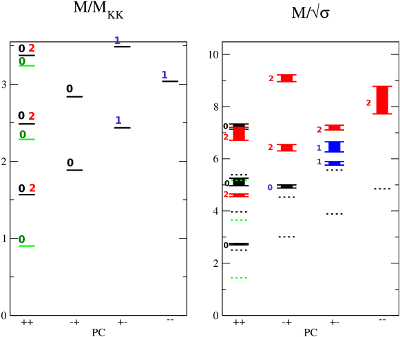
(a) (b)

Figure 1: The glueball spectrum of the Witten model (a) in units of $M_{\rm KK}$, (“exotic” scalar modes in green), compared to the spectrum obtained in the recent large-$N_{c}$ lattice calculations of Ref. Lucini et al. (2010) (b) in units of the square root of the string tension $\sqrt{\sigma}$, juxtaposed such that the lowest tensor mode is matched. The dotted lines in figure (b) give the glueball spectrum of the Witten model when expressed in terms of the string tension of the Witten model with the standard set of parameters (34) for the Sakai-Sugimoto model.

Mode	S4	T4	V4	N4	M4	L4
$J^{PC}$	$0^{++}$	$0^{++}/2^{++}$	$0^{-+}$	$1^{+-}$	$1^{--}$	$0^{++}$
n=0	7.30835	22.0966	31.9853	53.3758	83.0449	115.002
n=1	46.9855	55.5833	72.4793	109.446	143.581	189.632
n=2	94.4816	102.452	126.144	177.231	217.397	277.283
n=3	154.963	162.699	193.133	257.959	304.531	378.099
n=4	228.709	236.328	273.482	351.895	405.011	492.171

Table 2: Our results for the mass spectrum $m_{n}^{2}$ of AdS₇ black hole metric fluctuations in the notation of Brower et al. (2000) (i.e. in units of $r_{\rm KK}^{2}/L^{4}=M_{\rm KK}^{2}/9$) obtained by spectral methods cross-checked with a shooting method. The results for the lowest modes agree completely with Ref. Brower et al. (2000), while for certain higher modes there are deviations in the last few digits. $J^{PC}$ assignments are given only for the modes with even “$\tau$-parity” that are expected to have a counterpart in QCD.

II.2 Normalization of glueball modes

In order to be able to derive effective actions of the glueball modes and their interactions, we need to calculate the normalization factors required for a canonical kinetic term. For this purpose it is convenient to use the 11-dimensional notation, where the fluctuations take their simplest form.

II.2.1 Lowest (exotic) scalar glueball

The lowest scalar glueball $0^{++}$ is associated with fluctuations involving asymptotically (for $r\to\infty$) $\delta G_{44}=-4\delta G_{11}=-4\delta G_{22}=-4\delta G_{33}=-4\delta G_{11,11}$. In the bulk, other metric components are also involved, leading to the following “exotic polarization” Constable and Myers (1999)

$$\delta G_{44}=-\frac{r^{2}}{L^{2}}fH_{E}(r)G_{E}(x)$$

$$\delta G_{\mu\nu}=\frac{r^{2}}{L^{2}}H_{E}(r)\left[\frac{1}{4}\eta_{\mu\nu}-\left(\frac{1}{4}+\frac{3r_{\rm KK}^{6}}{5r^{6}-2r_{\rm KK}^{6}}\right)\frac{\partial_{\mu}\partial_{\nu}}{M_{E}^{2}}\right]G_{E}(x),$$

$$\delta G_{11,11}=\frac{r^{2}}{L^{2}}\frac{1}{4}H_{E}(r)G_{E}(x),$$

$$\delta G_{rr}=-\frac{L^{2}}{r^{2}}f^{-1}\frac{3r_{\rm KK}^{6}}{5r^{6}-2r_{\rm KK}^{6}}H_{E}(r)G_{E}(x),$$

$$\delta G_{r\mu}=\frac{90\,r^{7}r_{\rm KK}^{6}}{M_{E}^{2}L^{2}(5r^{6}-2r_{\rm KK}^{6})^{2}}H_{E}(r)\partial_{\mu}G_{E}(x),$$ (11)

where the eigenvalue equation is given by

$$\frac{1}{r^{3}}\frac{d}{dr}r(r^{6}-r_{\rm KK}^{6})\frac{d}{dr}H_{E}(r)+\left(\frac{432\,r^{2}\,r_{\rm KK}^{12}}{(5r^{6}-2r_{\rm KK}^{6})^{2}}+L^{4}M_{E}^{2}\right)H_{E}(r)=0.$$ (12)

Integration over the $S^{4}$ reduces the 11-dimensional supergravity action to

$$S=\frac{1}{2\kappa_{11}^{2}}(L/2)^{4}\Omega_{4}\int d^{7}x\sqrt{-\det G}\left(R(G)+\frac{30}{L^{2}}\right)$$ (13)

with $2\kappa_{11}^{2}=(2\pi)^{8}l_{s}^{9}g_{s}^{3}$ and $\Omega_{4}=8\pi^{2}/3$.

Inserting the metric fluctuations (II.2.1) into the 7-dimensional action gives

$$\int d^{7}x\sqrt{-\det G}\left.\left(R(G)+\frac{30}{L^{2}}\right)\right|_{H_{E}^{2}}$$ (14)

$$= -\mathcal{C}_{E}\int dx^{11}\,d^{4}x\,dx^{4}\,\frac{1}{2}\left[(\partial_{\mu}G_{E})^{2}+M_{E}^{2}G_{E}^{2}\right]$$

with

$$\mathcal{C}_{E}=\int_{r_{\rm KK}}^{\infty}\frac{dr\,r^{3}}{L^{3}}\frac{5}{8}H_{E}(r)^{2}.$$ (15)

For the lowest eigenmode $H_{E}$ we obtain numerically

$$\mathcal{C}_{E}=0.057395\,[H_{E}(r_{\rm KK})]^{2}\frac{r_{\rm KK}^{4}}{L^{3}}.$$ (16)

[This deviates from the result given in Ref. Hashimoto et al. (2008) by a factor $\frac{1}{2}$ that seems to be missing in their Eq. (2.19).]

Requiring that upon integration over $x^{4}$ and $x^{11}$ the scalar field $G_{E}(x)$ is canonically normalized leads to

$$[H_{E}(r_{\rm KK})]^{-1}=[H_{E}(Z\!=\!0)]^{-1} = \frac{1}{\sqrt{2}}0.0097839\,\lambda^{1/2}\,N_{c}\,M_{\rm KK}$$ (17)

$$= 0.0069183\,\lambda^{1/2}\,N_{c}\,M_{\rm KK}.$$

(This differs from Hashimoto et al. (2008) only by the explicitly written factor $1/{\sqrt{2}}$.)

II.2.2 Scalar and tensor modes from the tensor multiplet

A scalar mode $0^{++}$ that does not involve metric components with index 4 is obtained from

$$\delta G_{11,11} = -3\frac{r^{2}}{L^{2}}H_{D}(r)G_{D}(x)$$

$$\delta G_{\mu\nu} = \frac{r^{2}}{L^{2}}H_{D}(r)\left[\eta_{\mu\nu}-\frac{\partial_{\mu}\partial_{\nu}}{\Box}\right]G_{D}(x).$$ (18)

Since upon reduction to 10 dimensions $\delta G_{11,11}$ is essentially the dilaton, we shall refer to this mode as predominantly dilatonic. [Note that also the “exotic” mode (II.2.1) involves a dilaton component, but that there the dominant component is $\delta G_{44}$. It should also be kept in mind that the attribute “exotic” only refers to the holographic origin of this mode, and not to any exotic $J^{PC}$ quantum numbers in the dual field theory.]

The tensor glueball $2^{++}$ is dual to metric fluctuations that have neither $\delta G_{44}$ nor $\delta G_{11,11}$, but contain a transverse traceless polarization tensor in $\delta G_{\mu\nu}$. For example, one can choose as only nonvanishing components

$$\delta G_{11}=-\delta G_{22}=-\frac{r^{2}}{L^{2}}H_{T}(r)G_{T}(x).$$ (19)

The radial functions $H_{D,T}$ are determined by the equation

$$\frac{1}{r^{3}}\frac{d}{dr}r(r^{6}-r_{\rm KK}^{6})\frac{d}{dr}H_{D,T}(r)+L^{4}M^{2}H_{D,T}(r)=0,$$ (20)

with $M^{2}=M_{D}^{2}=M_{T}^{2}$.

Calculating the normalization of these glueball modes in analogy to (14) leads to

$$\mathcal{C}_{D,T}=\int_{r_{\rm KK}}^{\infty}\frac{dr\,r^{3}}{L^{3}}\left\{6H_{D}(r)^{2}\atop H_{T}(r)^{2}\right.$$ (21)

For the lowest eigenmode $H_{E}$ we obtain numerically

$$\mathcal{C}_{T}=0.22547\,[H_{T}(r_{\rm KK})]^{2}\frac{r_{\rm KK}^{4}}{L^{3}}$$ (22)

and an analogous result for $\mathcal{C}_{D}$ with a coefficient 6 times as large.

This leads to

$$[H_{D,T}(r_{\rm KK})]^{-1}=[H_{D,T}(Z\!=\!0)]^{-1}=\lambda^{1/2}\,N_{c}\,M_{\rm KK}\left\{0.033588\atop 0.013712\right.$$ (23)

II.3 Glueball field/operator correspondence

The above metric perturbations are sourced by operators in the dual field theory, which is five-dimensional super-Yang-Mills theory compactified on the circle along $x^{4}$.

The operator dual to the tensor perturbations is simply the five-dimensional energy-momentum tensor with three-dimensional indices. Omitting the adjoint scalars of the five-dimensional theory, we have

$$T_{mn}^{(5)}=T_{mn}^{\rm YM}+F_{4m}F_{4n}-\frac{1}{2}\delta_{mn}F_{4\mu}F_{4}{}^{\mu}+\ldots,$$ (24)

where $A_{4}$ is a further scalar that like the adjoint scalars of the five-dimensional theory becomes massive through loop corrections.

The operators dual to the exotic and the predominantly dilatonic scalar modes can be inferred from their couplings to the fields in the DBI action of D4 branes in the limit of $r\to\infty$ Hashimoto and Oz (1999). The exotic scalar mode $\delta G^{E}_{MN}$ and the dilatonic one, $\frac{1}{4}\delta G^{D}_{MN}$, turn out to source, respectively,

$$\mathcal{O}^{E} = -\frac{5}{8}F_{\mu\nu}F^{\mu\nu}-\frac{1}{2}T_{00}^{\rm YM}+F_{4\mu}F_{4}{}^{\mu}-\frac{1}{2}F_{40}^{2}+\ldots,$$ (25)

$$\mathcal{O}^{D} = +\frac{3}{8}F_{\mu\nu}F^{\mu\nu}-\frac{1}{2}T_{00}^{\rm YM}+F_{4\mu}F_{4}{}^{\mu}-\frac{1}{2}F_{40}^{2}+\ldots.$$ (26)

The difference $\mathcal{O}^{D}-\mathcal{O}^{E}=F_{\mu\nu}F^{\mu\nu}$ is the purely four-dimensional glueball operator, which is dual to $\frac{1}{4}\delta G^{D}_{MN}-\delta G^{E}_{MN}$. However this linear combination is not a normal mode in the gravitational background. We therefore need to keep the exotic and the predominantly dilatonic mode, of which both, or perhaps only one of them, might correspond to the glueballs of the four-dimensional Yang-Mills theory. To really end up with the latter, one would however need to take the limit of large Kaluza-Klein mass $M_{\rm KK}$, which is necessarily leaving the supergravity approximation. In this limit, both modes will presumably receive important corrections. If one of the modes drops out of the spectrum, one might suspect that it will more likely be $\delta G^{E}_{MN}$ as it includes a then spurious polarization component $\delta G_{44}$.

In the following we shall consider both modes, as well as the tensor mode, when calculating glueball-meson interactions within the Witten-Sakai-Sugimoto model, extending the analysis of Ref. Hashimoto et al. (2008), which only studied the lowest (exotic) $0^{++}$ mode.

III The Witten-Sakai-Sugimoto model

Sakai and Sugimoto introduced chiral quarks in Witten’s model of pure-glue Yang-Mills theory by means of $N_{f}$ probe D8 and anti-D8 branes that fill all spatial directions except the Kaluza-Klein circle Sakai and Sugimoto (2005a, b). Quarks and antiquarks are thus localized on separate points $x^{4}$ of the 4+1-dimensional boundary theory. The global flavor symmetry $\mathrm{U}(N_{f})_{L}\times\mathrm{U}(N_{f})_{R}$ is however broken spontaneously, because the subspace $x^{4}$-$U$ has the topology of a cigar forcing the D8 and anti-D8 branes to join in the bulk. The action of the joined D8 branes which describes the dynamics of $q\bar{q}$ mesons through flavor gauge fields on the branes reads

$$S_{\rm D8} = -T_{\rm D8}{\rm Tr}\,\int d^{9}xe^{-\Phi}\sqrt{-\det\left(\tilde{g}_{MN}+2\pi\alpha^{\prime}F_{MN}\right)}+S_{\rm CS}$$ (27)

$$=-(2\pi\alpha^{\prime})^{2}T_{\rm D8}{\rm Tr}\,\int d^{9}xe^{-\Phi}\sqrt{-\tilde{g}}\left(\mathbf{1}+\frac{1}{4}\tilde{g}^{PR}\tilde{g}^{QS}F_{PQ}F_{RS}+O(F^{4})\right)+S_{\rm CS}$$

with $T_{\rm D8}=(2\pi)^{-8}l_{s}^{-9}$, $\tilde{g}_{MN}$ the metric on the 8+1-dimensional world volume induced by (7), and $\Phi$ shifted such that $e^{\Phi}=g_{s}(U/R_{\rm D4})^{3/4}$. Because no backreaction of the D8 branes on the 10-dimensional background of the Witten model is taken into account, this corresponds to the quenched approximation of QCD, as indeed appropriate for the large-$N_{c}$ limit at fixed $N_{f}$. (For attempts to go beyond the quenched approximation see Refs. Burrington et al. (2008); Bigazzi and Cotrone (2014).)

In the original version of the Sakai-Sugimoto model that we shall use here, the D8 and anti-D8 branes are put at antipodal points so that they join at the minimal value $U=U_{\rm KK}$. In this case it is most convenient to use the dimensionless coordinate $Z=\sqrt{(U/U_{\rm KK})^{3}-1}$ introduced already above, but extended to the range $-\infty\ldots+\infty$ so that the radial integrations of the D8 and the anti-D8 branes are combined. The part of the DBI action quadratic in the flavor field strength then reads

$$S_{\rm D8}^{(F^{2})}=-\kappa\,{\rm Tr}\,\int d^{4}x\int_{-\infty}^{\infty}dZ\left[\frac{1}{2}K^{-1/3}\eta^{\mu\rho}\eta^{\nu\sigma}F_{\mu\nu}F_{\rho\sigma}+KM_{\rm KK}^{2}\eta^{\mu\nu}F_{\mu Z}F_{\nu Z}\right]$$ (28)

with $K\equiv 1+Z^{2}$ and

$$\kappa=(2\pi\alpha^{\prime})^{2}T_{\rm D8}g_{s}^{-1}\Omega_{4}\frac{1}{3}R_{\rm D4}^{9/2}U_{\rm KK}^{1/2}=\frac{\lambda N_{c}}{216\pi^{3}},$$ (29)

where (9) as well as $\Omega_{4}=8\pi^{2}/3$ and $M_{\rm KK}^{2}=(3/2)^{2}U_{\rm KK}/R_{\rm D4}^{3}$ have been used.

The Goldstone bosons of chiral symmetry breaking appear as

$$S_{\rm D8}=\frac{f_{\pi}^{2}}{4}\int d^{4}x\,{\rm Tr}\,\left(U^{-1}\partial_{\mu}U\right)^{2}+\ldots,\quad U=\mathrm{P}\exp\left\{i\int_{-\infty}^{\infty}dZA_{Z}\right\},$$ (30)

which determines the so-called pion decay constant in terms of $\lambda$ and $M_{\rm KK}$ as

$$f_{\pi}^{2}=\frac{1}{54\pi^{4}}\lambda N_{c}M_{\rm KK}^{2}.$$ (31)

Massive vector and axial vector mesons arise as even and odd eigenmodes of $A_{\mu}^{(n)}=\psi_{n}(Z)v^{(n)}_{\mu}(x)$ with eigenvalue equation

$$-(1+Z^{2})^{1/3}\partial_{Z}\left((1+Z^{2})\partial_{Z}\psi_{n}\right)=\lambda_{n}\psi_{n},\quad\psi_{n}(\pm\infty)=0.$$ (32)

The lowest mode $v_{\mu}^{(1)}$ is interpreted as the isotriplet $\rho$ meson (or the $\omega$ meson for the U(1) generator) with mass $m_{\rho}^{2}=\lambda_{1}M_{\rm KK}$ with the numerical result $\lambda_{1}=0.669314\ldots$.

The next-highest mode $v_{\mu}^{(2)}$ with eigenvalue $\lambda_{2}\approx 1.569$ is an axial vector that can be identified Sakai and Sugimoto (2005a) with the meson $a_{1}(1260)$. The experimental value for the ratio $m_{a_{1}}/m_{\rho}\approx 1.59$ is remarkably close to $\sqrt{(}\lambda_{2}/\lambda_{1})\approx 1.53$. Also the experimental value for the mass of the excited $\rho(1450)$ with $m_{\rho^{*}}/m_{\rho}\approx 1.89$ is is close to $\sqrt{(}\lambda_{3}/\lambda_{1})\approx 2.07$. This nice agreement may however be a bit fortuitous, since recent lattice simulations Bali et al. (2013) at large $N_{c}$, extrapolated to zero quark mass, give the higher values $m_{a_{1}}/m_{\rho}\approx 1.86$ and $m_{\rho^{*}}/m_{\rho}\approx 2.40$. This would correspond to errors 21% and 16%, respectively, which may still be considered a success given that already the mass of $v_{\mu}^{(2)}$ is above $M_{\rm KK}$. (For more checks of the quantitative predictions of the Witten-Sakai-Sugimoto model see Ref. Rebhan (2015).) Optimistically, one can therefore hope that the Witten-Sakai-Sugimoto model is a useful approximation to QCD up to masses of two or three times $M_{\rm KK}$.

III.1 Choice of parameters

Matching the result for the $\rho$ meson mass with its experimental value, $m_{\rho}=\sqrt{\lambda_{1}}M_{\rm KK}\approx 776$ MeV, fixes the Kaluza-Klein mass to Sakai and Sugimoto (2005a, b) $M_{\rm KK}=949$ MeV. This determines the masses of the other vector and axial vector mesons, which come out in rough agreement with experiment. The masses of the lowest (exotic) and the predominantly dilatonic scalar glueball, the tensor glueball (degenerate with the dilatonic scalar), and the lowest pseudoscalar glueball are fixed to, respectively,

$$M_{E}=\sqrt{7.30834/9}\,M_{\rm KK}\approx 855\,{\rm MeV},$$

$$M_{D}=M_{T}=\sqrt{22.0966/9}\,M_{\rm KK}\approx 1487\,{\rm MeV},$$

$$M_{P}=\sqrt{31.9853/9}\,M_{\rm KK}\approx 1789\,{\rm MeV},$$

$$M_{E^{*}}=\sqrt{46.9855/9}\,M_{\rm KK}\approx 2168\,{\rm MeV},$$

$$M_{D^{*}}=M_{T^{*}}=\sqrt{55.5833/9}\,M_{\rm KK}\approx 2358\,{\rm MeV},$$ (33)

where we have also given the masses of some of the corresponding excited states (marked by a star).

The lowest scalar glueball involving the exotic polarization (II.2.1) with a dominant $\delta G_{44}$ component is found to be only 10% heavier than the $\rho$ meson. This is in stark contrast to lattice results both for quenched $N_{c}=3$ and $N_{c}=\infty$ QCD Lucini et al. (2010), where the lightest glueball is about twice as heavy.

A possible modification of the Sakai-Sugimoto model consists of choosing a nonmaximal separation of the D8-$\overline{\rm D8}$ branes Antonyan et al. (2006); Aharony et al. (2007). The latter then join at a value $U=U_{0}>U_{\rm KK}$ and the mass of a string stretched between $U_{\rm KK}$ and $U_{0}$ has been interpreted as a “constituent” quark mass. Unfortunately, this only makes the problem worse: Nonmaximal separation increases the eigenvalue $\lambda_{1}$ Peeters and Zamaklar (2007) while the glueball spectrum is unaffected. With a constituent quark mass of 310 MeV and keeping the mass of the $\rho$ meson fixed as done in Ref. Callebaut et al. (2013), $M_{\rm KK}$ is reduced to 720 MeV, which reduces all values in (III.1) by 25%.

With maximal separation and the standard choice $M_{\rm KK}=949$ MeV, the mass of the dilatonic glueball is not far from the numerical result obtained in lattice gauge theory for the lightest scalar glueball state, while a degeneracy with the tensor glueball is not observed there—the latter is instead significantly heavier. This degeneracy might perhaps be lifted by higher-derivative corrections when going beyond the leading supergravity approximation. Similarly, it is conceivable that only the dilatonic glueball survives in the (unfortunately inaccessible) limit to a complete holographic QCD and that therefore the lowest scalar mode is to be discarded. We shall come back to this question when calculating the decay width of the various glueball states.

In order to calculate glueball-meson interactions, we shall need to extrapolate to finite coupling and finite $N_{c}=3$. The original Sakai and Sugimoto (2005a, b) and most widely used choice is obtained from matching $f_{\pi}\approx 92.4\,{\rm MeV}$ in (31) which gives

$$\kappa\equiv\lambda N_{c}/(216\pi^{3})=7.45\cdot 10^{-3}\;\Rightarrow\;\lambda\approx 16.63\quad(N_{c}=3).$$ (34)

[The original and published version of Ref. Sakai and Sugimoto (2005a, b) contained an error in the prefactor of the D8 brane action for $N_{f}>1$ involving a different definition of $\kappa$, which led to a ’t Hooft coupling of about 8.3 and effectively a correspondingly reduced pion decay constant. This error, which was later corrected in the e-print versions of Ref. Sakai and Sugimoto (2005a, b), did not affect the mass spectra of mesons obtained in Ref. Sakai and Sugimoto (2005a, b), but it does affect all interactions. Unfortunately, Ref. Hashimoto et al. (2008) still employed the incorrectly matched ’t Hooft coupling, affecting all meson and glueball decay rates calculated therein.]

In what follows, we shall take (34) as the standard choice, but also consider as an alternative a value of the ’t Hooft coupling obtained by matching $m_{\rho}/\sqrt{\sigma}$, where $\sigma$ is the string tension (10), to the large-$N_{c}$ lattice result of Ref. Bali et al. (2013). Ref. Bali et al. (2013) obtained $m_{\rho}/\sqrt{\sigma}=1.504(50)$, whose central value corresponds to $\lambda=12.55$. With the “standard” value $\lambda\approx 16.63$ the Sakai-Sugimoto model predicts $m_{\rho}/\sqrt{\sigma}\approx 1.306$, which agrees within 15% but points to a smaller ’t Hooft coupling and thus a smaller string tension. A smaller ’t Hooft coupling has also been argued for in Ref. Imoto et al. (2010), where the spectrum of higher-spin mesons obtained from massive open string modes has been considered. We shall therefore consider a downward variation of $\lambda\approx 16.63\ldots 12.55$ to get an idea of the variability of the predictions of the Witten-Sakai-Sugimoto model.

Before turning to decay rates, we consider two other predictions of the Witten-Sakai-Sugimoto model at finite $N_{c}$ where the concrete value of $\lambda$ matters.

At infinite $N_{c}$, the Goldstone bosons include also a massless $\eta^{\prime}$ pseudoscalar meson from the spontaneous breaking of the $\mathrm{U}_{A}(1)$ symmetry, whose anomaly is suppressed at $N_{c}\to\infty$. However, at finite $N_{c}$, the Sakai-Sugimoto model predicts a finite mass for the $\eta^{\prime}$ meson through a Witten-Veneziano formula evaluated already in Sakai and Sugimoto (2005a) with the result

$$m_{\eta^{\prime}}=\frac{1}{3\sqrt{3}\pi}\sqrt{\frac{N_{f}}{N_{c}}}\lambda M_{\rm KK}.$$ (35)

With $M_{\rm KK}=949$ MeV and $\lambda\approx 16.63$ (or 12.55) the numerical value for $N_{c}=N_{f}=3$ turns out to be 967 MeV (730 MeV). The higher value is surprisingly close to the experimental value 958 MeV, but actually a smaller value than that might perhaps be expected given the absence of a strange quark mass. At any rate, the right ballpark seems to be reached with the parameters considered here.

Another quantity of interest, in particular in connection with glueball physics, is the gluon condensate which was calculated in Ref. Kanitscheider et al. (2008) as

$$C^{4}\equiv\left<\frac{\alpha_{s}}{\pi}G_{\mu\nu}^{a}G^{a\mu\nu}\right>=\frac{4N_{c}}{3^{7}\pi^{4}}\lambda^{2}M_{\rm KK}^{4}.$$ (36)

For $\lambda\approx 16.63$ this yields $C^{4}=0.0126\,{\rm GeV}^{4}$, almost identical to the standard SVZ sum rule value Shifman et al. (1979), while for $\lambda=12.55$ a significantly smaller value of 0.0072 GeV⁴ is obtained. Using sum rules both smaller Ioffe (2006) and larger Narison (2012) values than the standard SVZ sum rule value are discussed in the literature, while lattice simulations typically give significantly larger values, which are however of the same size as ambiguities from the subtraction procedure Bali et al. (2014). While a quantitative comparison thus does not seem to be in order, we note that the gluon condensate is predicted to be small.

III.2 Normalization of $q\bar{q}$ modes

For the calculation of decay rates we will initially consider $N_{f}=2$, dropping the strange quark whose nonnegligible mass cannot be easily accommodated within the Sakai-Sugimoto model (see however Ref. Bergman et al. (2007); Aharony and Kutasov (2008); Hashimoto et al. (2008); McNees et al. (2008)); the possible effects of the finite quark masses will be discussed in Section V.

In the chiral Sakai-Sugimoto model, the Goldstone bosons are the massless pions contained in

$$A_{Z}=U_{\rm KK}\phi_{0}(Z)\pi(x^{\mu}),$$ (37)

where $U_{\rm KK}$ has been included to render the mode function $\phi_{0}(Z)$ dimensionless. The U(1) part of $A_{Z}$ corresponds to the $\eta^{\prime}$ meson, which is a Goldstone boson only at infinite $N_{c}$; for finite $N_{c}$ it receives a mass through the Witten-Veneziano mechanism Sakai and Sugimoto (2005a) (see Eq. (35) below).

The only vector mesons that we shall consider will be the isotriplet $\rho$ meson described by the traceless part of

$$A_{\mu}=\psi_{1}(Z)\rho_{\mu}(x^{\nu}),$$ (38)

and the isosinglet $\omega$ meson given by the corresponding expression proportional to the unit matrix.

Following Ref. Hashimoto et al. (2008) (which here differs from Sakai and Sugimoto (2005a, b)) we choose the generators of the SU(2) flavor group such that ${\rm Tr}\,T^{a}T^{b}=\delta^{ab}$. Canonical normalization of the fields $\pi^{a}$ and $\rho^{a}_{\mu}$ in (28) such that upon integration over $Z$ one has

$$S=-{\rm Tr}\,\int d^{4}x\left[\frac{1}{2}(\partial_{\mu}\pi)^{2}+\frac{1}{4}F_{\mu\nu}^{2}+\frac{1}{2}\lambda_{1}M_{\rm KK}^{2}\rho_{\mu}^{2}+\ldots\right]$$ (39)

leads to

$$2\kappa\int_{-\infty}^{\infty}dZ\,K^{-1/3}(\psi_{1})^{2}=1,$$ (40)

$$2\kappa(U_{\rm KK}M_{\rm KK})^{2}\int_{-\infty}^{\infty}dZ\,K(\phi_{0})^{2}=1.$$ (41)

The first relation determines the value of $\psi_{1}$ at $Z=0$ with the help of the numerical result

$$\int_{-\infty}^{\infty}dZ\,K^{-1/3}(\psi_{1})^{2}=2.80302\ldots\,\psi_{1}^{2}(0),$$ (42)

while the second fixes the normalization of $\phi_{0}\propto 1/K\equiv 1/(1+Z^{2})$ as

$$U_{\rm KK}M_{\rm KK}\,\phi_{0}=\frac{1}{\sqrt{2\pi\kappa}}\frac{1}{K}.$$ (43)

III.3 $\rho$ and $\omega$ meson decay

The $\rho$-$\pi$ interactions are determined by the second term of (28), using $F_{\mu Z}=\partial_{\mu}A_{Z}-\partial_{Z}A_{\mu}-i[A_{\mu},A_{Z}]$. The effective vertex between the four-dimensional fields $\rho$ and $\pi$’s are obtained upon integration of the resulting products of the mode functions $\psi_{1}(Z)$ and $\phi_{0}\propto 1/K$. For the process $\rho\to\pi\pi$ we need specifically

$$\mathcal{L}_{\rho\pi\pi}=-g_{\rho\pi\pi}\epsilon_{abc}(\partial_{\mu}\pi^{a})\rho^{b\mu}\pi^{c},\quad g_{\rho\pi\pi}=\sqrt{2}\int dZ\frac{1}{\pi K}\psi_{1}=\sqrt{2}\times 24.030\,\lambda^{-\frac{1}{2}}N_{c}^{-\frac{1}{2}}.$$ (44)

This agrees with the numerical value given in table 3$\cdot$34 of Ref. Sakai and Sugimoto (2005b) for $g_{v^{1}\pi\pi}\equiv g_{\rho\pi\pi}$. ($g_{\rho\pi\pi}/\sqrt{2}$ was denoted as $c_{6}$ in Hashimoto et al. (2008); we will reserve $c_{i}$, $i=1,2,3\ldots$, for the coefficients in the interactions of the glueball field with mesons, for which we will follow the conventions chosen in Hashimoto et al. (2008).)

The amplitude for the decay of a $\rho$ meson at rest with polarization $\epsilon^{\mu}=(0,\mathbf{e})$ into two pions with momenta $p^{\mu}=(|\mathbf{p}|,\mathbf{p})$ and $q^{\mu}=(|\mathbf{p}|,-\mathbf{p})$ reads

$$\mathcal{M}=ig_{\rho\pi\pi}\,\epsilon^{\mu}(p_{\mu}-q_{\mu})=2ig_{\rho\pi\pi}\,\mathbf{e}\cdot\mathbf{p}.$$ (45)

The expression for the decay rate involves a directional average, leading to

$$\Gamma_{\rho}/m_{\rho}=\frac{1}{4\pi}\int d\Omega\frac{|\mathcal{M}|^{2}}{16\pi m_{\rho}^{2}}=\frac{g_{\rho\pi\pi}^{2}}{48\pi}\approx\frac{7.659}{\lambda N_{c}}\approx\left\{0.1535\;(\lambda=16.63)\atop 0.2034\;(\lambda=12.55)\right.$$ (46)

which compares remarkably well with the current experimental value $\Gamma_{\rho}/m_{\rho}=0.191(1)$ from Ref. Olive et al. (2014) (although it should be noted that in this process the finite pion mass implies a reduction by about 20% compared to a decay into massless particles so that the coupling $g_{\rho\pi\pi}$ appears somewhat underestimated with our range of parameters for the Sakai-Sugimoto model).

The decay of the $\omega$ meson into $\pi^{0}\gamma$ and $\pi^{0}\pi^{+}\pi^{-}$, which is due to the Chern-Simons part of the D8 brane action, has been calculated in Sakai and Sugimoto (2005b), with the result $2.58$ MeV for the dominant 3-pion decay, which is significantly below the experimental value $\approx 7.6$ MeV. However, the result of Sakai and Sugimoto (2005b) is proportional to $\lambda^{-4}$. Varying again $\lambda$ from 16.63 to 12.55 gives the range 2.58…7.96 MeV, which happens to include the experimental value.

So the model appears to make reasonable semi-quantitative estimates for meson interactions, which is quite remarkable given that after fixing the mass scale and setting $N_{c}=3$, there is only one free parameter, namely $\lambda$. This certainly makes it interesting to consider the predictions of this model for glueball decay rates in detail.

IV Glueball-meson interactions

The glueball modes, which have been obtained in Sect. II.1 in terms of 11-dimensional metric perturbations $\delta G_{\hat{M}\hat{N}}$, translate to perturbations of the type-IIA string metric $g_{MN}$ and the dilaton $\Phi$ according to (5). Explicitly, this gives

$$g_{\mu\nu} = \frac{r^{3}}{L^{3}}\left[\left(1+\frac{L^{2}}{2r^{2}}\delta G_{11,11}\right)\eta_{\mu\nu}+\frac{L^{2}}{r^{2}}\delta G_{\mu\nu}\right],$$

$$g_{44} = \frac{r^{3}f}{L^{3}}\left(1+\frac{L^{2}}{2r^{2}}\delta G_{11,11}+\frac{L^{2}}{r^{2}f}\delta G_{44}\right),$$

$$g_{rr} = \frac{L}{rf}\left(1+\frac{L^{2}}{2r^{2}}\delta G_{11,11}+\frac{r^{2}f}{L^{2}}\delta G_{rr}\right),$$

$$g_{r\mu} = \frac{r}{L}\delta G_{r\mu},$$

$$g_{\Omega\Omega} = \frac{r}{L}\left(\frac{L}{2}\right)^{2}\left(1+\frac{L^{2}}{2r^{2}}\delta G_{11,11}\right),$$

$$e^{4\Phi/3} = \frac{r^{2}}{L^{2}}\left(1+\frac{L^{2}}{r^{2}}\delta G_{11,11}\right).$$ (47)

Here we differ from Ref. Hashimoto et al. (2008) where the metric fluctuations $g_{\Omega\Omega}$ on the $S^{4}$ have been omitted. As one can check (Appendix A), the 10-dimensional equations for the glueball modes are satisfied only when the fluctuation in $g_{\Omega\Omega}$ is kept.

We shall consider in turn the lowest glueball dual to the metric fluctuations (II.2.1), referred to as “exotic” because it involves $\delta G_{44}$ besides dilaton fluctuations in $\delta G_{11,11}$, the predominantly dilatonic glueball associated to (II.2.2), and the tensor glueball with metric fluctuations (19). Inserting the respective metric fluctuations in the D8 brane action and integrating over the bulk coordinates yields effective interaction Lagrangians which are given in full detail in Appendix B.

IV.1 Glueball decay to two pions

Figure 2: Leading-order glueball decay into two pions.

The effective, 3+1-dimensional interaction Lagrangian for the lowest (exotic) $0^{++}$ glueball $G_{E}$ reads (omitting terms that vanish when $G_{E}$ is on-shell)

$$\mathcal{L}^{G_{E}\to\pi\pi}=-{\rm Tr}\,\left[\frac{1}{2}c_{1}\partial_{\mu}\pi\partial_{\nu}\pi\frac{\partial^{\mu}\partial^{\nu}}{M_{E}^{2}}G_{E}+\frac{1}{2}\breve{c}_{1}\partial_{\mu}\pi\partial^{\mu}\pi\,G_{E}\right]$$ (48)

with coupling constants $c_{1}$ and $\breve{c}_{1}$ defined in (B.1) and numerically given in Table 3.

	vertex	value
$c_{1}/\sqrt{2}$	$G_{E}\partial\pi\partial\pi$	$44.304\;\lambda^{-\frac{1}{2}}\,N_{c}^{-1}M_{\rm KK}^{-1}$
$c_{2}/\sqrt{2}$	$G_{E}\rho\rho$	$5.0318\;\lambda^{-\frac{1}{2}}\,N_{c}^{-1}M_{\rm KK}^{-1}$
$c_{3}/\sqrt{2}$	$G_{E}\partial\rho\partial\rho$	$49.334\;\lambda^{-\frac{1}{2}}\,N_{c}^{-1}M_{\rm KK}^{-1}$
$c_{4}/\sqrt{2}$	$G_{E}\rho\partial\rho$	$-7.4810\;\lambda^{-\frac{1}{2}}\,N_{c}^{-1}M_{\rm KK}^{+1}$
$c_{5}/\sqrt{2}$	$G_{E}\rho\pi\partial\pi$	$1428.1\;\lambda^{-1}\,N_{c}^{-\frac{3}{2}}M_{\rm KK}^{-1}$
$\breve{c}_{1}/\sqrt{2}$	$G_{E}\partial\pi\partial\pi$	$11.590\;\lambda^{-\frac{1}{2}}\,N_{c}^{-1}M_{\rm KK}^{-1}$
$\breve{c}_{2}/\sqrt{2}$	$G_{E}\rho\rho$	$2.0970\;\lambda^{-\frac{1}{2}}\,N_{c}^{-1}M_{\rm KK}^{-1}$
$\breve{c}_{3}/\sqrt{2}$	$G_{E}\partial\rho\partial\rho$	$12.814\;\lambda^{-\frac{1}{2}}\,N_{c}^{-1}M_{\rm KK}^{-1}$
$\breve{c}_{5}/\sqrt{2}$	$G_{E}\rho\pi\partial\pi$	$359.33\;\lambda^{-1}\,N_{c}^{-\frac{3}{2}}M_{\rm KK}^{-1}$
$c_{1}^{*}/\sqrt{2}$	$G_{E}^{*}\partial\pi\partial\pi$	$24.641\;\lambda^{-\frac{1}{2}}\,N_{c}^{-1}M_{\rm KK}^{-1}$
$c^{*}_{2}/\sqrt{2}$	$G_{E}^{*}\rho\rho$	$-0.8227\;\lambda^{-\frac{1}{2}}\,N_{c}^{-1}M_{\rm KK}^{-1}$
$c^{*}_{3}/\sqrt{2}$	$G_{E}^{*}\partial\rho\partial\rho$	$27.906\;\lambda^{-\frac{1}{2}}\,N_{c}^{-1}M_{\rm KK}^{-1}$
$c^{*}_{4}/\sqrt{2}$	$G_{E}^{*}\rho\partial\rho$	$-1.7467\;\lambda^{-\frac{1}{2}}\,N_{c}^{-1}M_{\rm KK}^{+1}$
$c^{*}_{5}/\sqrt{2}$	$G_{E}^{*}\rho\pi\partial\pi$	$858.66\;\lambda^{-1}\,N_{c}^{-\frac{3}{2}}M_{\rm KK}^{-1}$
$\breve{c}^{*}_{1}/\sqrt{2}$	$G_{E}^{*}\partial\pi\partial\pi$	$4.5843\;\lambda^{-\frac{1}{2}}\,N_{c}^{-1}M_{\rm KK}^{-1}$
$\breve{c}^{*}_{2}/\sqrt{2}$	$G_{E}^{*}\rho\rho$	$-1.2390\;\lambda^{-\frac{1}{2}}\,N_{c}^{-1}M_{\rm KK}^{-1}$
$\breve{c}^{*}_{3}/\sqrt{2}$	$G_{E}^{*}\partial\rho\partial\rho$	$5.3829\;\lambda^{-\frac{1}{2}}\,N_{c}^{-1}M_{\rm KK}^{-1}$
$\breve{c}^{*}_{5}/\sqrt{2}$	$G_{E}^{*}\rho\pi\partial\pi$	$176.99\;\lambda^{-1}\,N_{c}^{-\frac{3}{2}}M_{\rm KK}^{-1}$

Table 3: Coupling coefficients in interaction Lagrangian of lowest glueball. (Here we give numerical results for $c_{i}/\sqrt{2}$ to permit a comparison with the results listed in Hashimoto et al. (2008), with which we disagree by a factor of $\sqrt{2}$ in (17). Taking this into account we agree with all numerical values, with the exception of $c_{4}$, which in Hashimoto et al. (2008) seems to be missing the numerical factor contained in the normalization of $H_{E}(Z)$.) The coefficients $\breve{c}_{1,2,3,5}$ are coupling constants due to $S_{4}$ volume fluctuations induced by the lowest glueball that were apparently dropped in Hashimoto et al. (2008). Coefficients with a star indicate the corresponding constants for the first excited exotic mode.

	vertex	value
$d_{1}$	$\tilde{G}\partial\pi\partial\pi$	$17.226\;\lambda^{-\frac{1}{2}}\,N_{c}^{-1}M_{\rm KK}^{-1}$
$d_{2}$	$\tilde{G}\rho\rho$	$4.3714\;\lambda^{-\frac{1}{2}}\,N_{c}^{-1}M_{\rm KK}^{-1}$
$d_{3}$	$\tilde{G}\partial\rho\partial\rho$	$18.873\;\lambda^{-\frac{1}{2}}\,N_{c}^{-1}M_{\rm KK}^{-1}$
$d_{5}$	$\tilde{G}\rho\pi\partial\pi$	$512.20\;\lambda^{-1}\,N_{c}^{-\frac{3}{2}}M_{\rm KK}^{-1}$
$d^{*}_{1}$	$\tilde{G}^{*}\partial\pi\partial\pi$	$11.906\;\lambda^{-\frac{1}{2}}\,N_{c}^{-1}M_{\rm KK}^{-1}$
$d^{*}_{2}$	$\tilde{G}^{*}\rho\rho$	$-0.9415\;\lambda^{-\frac{1}{2}}\,N_{c}^{-1}M_{\rm KK}^{-1}$
$d^{*}_{3}$	$\tilde{G}^{*}\partial\rho\partial\rho$	$13.680\;\lambda^{-\frac{1}{2}}\,N_{c}^{-1}M_{\rm KK}^{-1}$
$d^{*}_{5}$	$\tilde{G}^{*}\rho\pi\partial\pi$	$419.46\;\lambda^{-1}\,N_{c}^{-\frac{3}{2}}M_{\rm KK}^{-1}$

Table 4: Coupling coefficients $d_{i}$ ($t_{i}\equiv\sqrt{6}\,d_{i}$) in the interaction Lagrangian of the lowest glueballs in the tensor multiplet (dilaton and tensor), collectively denoted as $\tilde{G}$, with a star indicating the first excited mode. (Note that there is no term analogous to the one involving $c_{4}$ for the lowest (exotic) glueball.)

The corresponding result for the dilatonic scalar $0^{++}$ and the $2^{++}$ mode, denoted $G_{D}$ and $T^{\mu\nu}$, respectively, is

$$\mathcal{L}^{G_{D}\to\pi\pi} = \frac{1}{2}d_{1}{\rm Tr}\,\partial_{\mu}\pi\partial_{\nu}\pi\left(\eta^{\mu\nu}-\frac{\partial^{\mu}\partial^{\nu}}{M_{D}^{2}}\right)G_{D},$$ (49)

$$\mathcal{L}^{G_{T}\to\pi\pi} = \frac{1}{2}t_{1}{\rm Tr}\,\partial_{\mu}\pi\partial_{\nu}\pi\,T^{\mu\nu},\quad t_{1}\equiv\sqrt{6}\,d_{1}.$$ (50)

$G_{D}$ is a canonically normalized real scalar, and $T^{\mu\nu}$ a massive tensor field with transverse traceless polarizations, normalized such that

$$\mathcal{L}^{T}=\frac{1}{4}T_{\mu\nu}(\Box-M_{T}^{2})T^{\mu\nu}+B_{\mu}\partial_{\nu}T^{\mu\nu}+B\eta_{\mu\nu}T^{\mu\nu}+\ldots,$$ (51)

where $B_{\mu}$ and $B$ are Lagrange multiplier fields. The coefficient $d_{1}$ is given in Table 4.

For the two scalar glueballs described by $G_{E}$ and $G_{D}$, the decay width into two pions is given by the simple expression

$$\Gamma_{G_{E,D}\to\pi\pi}=\frac{|\mathbf{p}|}{8\pi M^{2}_{E,D}}|\mathcal{M}_{E,D}|^{2}\times 3\times\frac{1}{2},$$ (52)

where $\mathbf{p}$ is the momentum of one of the pions in the rest frame of the glueball with $|\mathbf{p}|=M_{E,D}/2$, the factor of 3 comes from the sum over the isospin quantum number, and the factor of $\frac{1}{2}$ is included because the two pions are identical. The amplitude for the decay of $G_{E}$ and $G_{D}$ is, respectively,

$$|\mathcal{M}_{E}| = |(c_{1}+\breve{c}_{1})p_{0}q_{0}-\breve{c}_{1}\mathbf{p}\cdot\mathbf{q}|=|c_{1}+2\breve{c}_{1}|\frac{M^{2}_{E}}{4},$$ (53)

$$\quad|\mathcal{M}_{D}| = |d_{1}\mathbf{p}\cdot\mathbf{q}|=|d_{1}|\frac{M^{2}_{D}}{4}.$$ (54)

For the tensor glueball an average over the polarizations of the tensor is needed. Alternatively, we can choose a fixed polarization $\epsilon^{11}=-\epsilon^{22}=1$ and integrate over the orientation of our Cartesian coordinates. This leads to the scattering amplitude (in the rest frame of the tensor glueball)

$$|\mathcal{M}_{T}|=|t_{1}(p_{x}^{2}-p_{y}^{2})|,\quad|\mathbf{p}|=M_{T}/2,$$ (55)

and the decay width

$$\Gamma_{T\to\pi\pi}=\frac{|\mathbf{p}|}{8\pi M_{T}^{2}}\int\frac{d\Omega}{4\pi}|\mathcal{M}_{T}|^{2}\times\frac{3}{2}=\frac{1}{640\pi}|t_{1}|^{2}M_{T}^{3}.$$ (56)

Numerically we obtain with $\lambda\approx 16.63$ for the scalar glueballs $G_{E}$, $G_{D}$, and $G_{D}^{*}$

$$\Gamma_{G_{E}\to\pi\pi}/M_{E} = \frac{3|c_{1}+2\breve{c}_{1}|^{2}M_{E}^{2}}{512\pi}\approx\frac{13.79}{\lambda N_{c}^{2}}\approx 0.092\quad(M_{E}\approx 855{\rm MeV})$$ (57)

$$\Gamma_{G_{D}\to\pi\pi}/M_{D} = \frac{3|d_{1}|^{2}M_{D}^{2}}{512\pi}\approx\frac{1.359}{\lambda N_{c}^{2}}\approx 0.009\quad(M_{D}\approx 1487{\rm MeV})$$ (58)

$$\Gamma_{G_{D}^{*}\to\pi\pi}/M_{D^{*}} = \frac{3|d^{*}_{1}|^{2}M_{D^{*}}^{2}}{512\pi}\approx\frac{1.633}{\lambda N_{c}^{2}}\approx 0.011\quad(M_{D^{*}}\approx 2358{\rm MeV})$$ (59)

and for the tensor

$$\Gamma_{T\to\pi\pi}/M_{T} = \frac{|t_{1}|^{2}M_{T}^{2}}{640\pi}\approx\frac{2.174}{\lambda N_{c}^{2}}\approx 0.0145\quad(M_{T}\approx 1487{\rm MeV})$$ (60)

$$\Gamma_{T^{*}\to\pi\pi}/M_{T^{*}} = \frac{|t_{1}^{*}|^{2}M_{T^{*}}^{2}}{640\pi}\approx\frac{2.613}{\lambda N_{c}^{2}}\approx 0.0175\quad(M_{T^{*}}\approx 2358{\rm MeV})$$ (61)

If we replace the standard choice $\lambda\approx 16.63$ by the smaller value 12.55 as discussed above, all these decay rates which are proportional to $\lambda^{-1}$ increase by 33% (see Table 5 for a summary).

	$M$	$\Gamma/M$
$G_{E}\to 2\pi$	855	0.092 …0.122
$G_{E}^{*}\to 2\pi$	2168	0.149 …0.197
$G_{D}\to 2\pi$	1487	0.009 …0.012
$G_{D}^{*}\to 2\pi$	2358	0.011 …0.014
$T\to 2\pi$	1487	0.0145 …0.0193
$T^{*}\to 2\pi$	2358	0.0175 …0.0233

Table 5: Decay width of scalar and tensor glueballs into 2 (massless) pions divided by glueball mass for $\lambda=16.63\ldots 12.55$

A somewhat anomalous feature of the lowest (exotic) scalar glueball is that its width is much larger than the next-to-lowest (dilatonic) scalar glueball while having a rather low mass. This appears rather unnatural if the dilatonic scalar glueball is interpreted as an excited scalar glueball and may be another indication that the exotic mode should be discarded altogether.

Interestingly enough, a scenario with a broad glueball around 1 GeV in combination with a narrow glueball in the range predicted by quenched (as well as unquenched Gregory et al. (2012)) lattice gauge theory has been proposed in Ref. Narison (1998, 2006); Mennessier et al. (2008); Kaminski et al. (2009) on the basis of QCD spectral sum rules. There the lighter glueball, called $\sigma_{\rm B}$, plays the role of an important bare glueball component of the $\sigma$-meson $f_{0}(500)$, while a higher narrow glueball around 1.5-1.6 GeV is required by the consistency of subtracted and unsubtracted sum rules. The glueball state $\sigma_{\rm B}$ of Ref. Narison (1998, 2006); Kaminski et al. (2009) has a broad decay width into two pions, in fact even much broader than (57), which makes us speculate that the exotic scalar glueball of the Witten-Sakai-Sugimoto model could find a role as the holographic dual of a pure-glue component of the $\sigma$-meson, perhaps while having to be discarded from the spectrum of the pure pure-glue Witten model. This would also be in line with the fact that the gluon condensate of the Witten model, Eq. (36), is small, close to its standard SVZ value Shifman et al. (1979), while models with only one scalar glueball field Ellis and Lanik (1985); Janowski et al. (2014) cannot reconcile a small gluon condensate with narrow glueball states.

In the range 1.5-1.8 GeV, where lattice gauge theory locates the lowest scalar glueball, there are, experimentally, two isoscalar mesons $f_{0}(1500)$ and $f_{0}(1710)$ which are frequently and alternatingly considered as predominantly glue. The experimental results for the decay width into two pions are

$$\Gamma^{\rm(ex)}(f_{0}(1500)\to\pi\pi)/(1505{\rm MeV})=0.025(3),$$ (62)

$$\Gamma^{\rm(ex)}(f_{0}(1710)\to\pi\pi)/(1722{\rm MeV})=\left\{0.017(4)\atop 0.009(2)\right.$$ (63)

where the first result is taken from Ref. Olive et al. (2014), the second from Ref. Parganlija (2012) using data from the BES collaboration Ablikim et al. (2006) (upper entry) and the WA102 collaboration Barberis et al. (1999) (lower entry), respectively.

The lowest (exotic) scalar glueball mode $G_{E}$ appears to have a much too large decay width to be consistent with a dominantly glueball interpretation of either $f_{0}(1500)$ or $f_{0}(1710)$. On the other hand, the dilatonic mode has a decay width below but comparable to the data for the two glueball candidates; in the case of the WA102 data for the $f_{0}(1710)$ there happens to be even complete agreement. In order to get a more complete picture, we shall now consider also the other couplings between glueballs and mesons as determined by the Witten-Sakai-Sugimoto model.

IV.2 Glueball decay to four and more pions

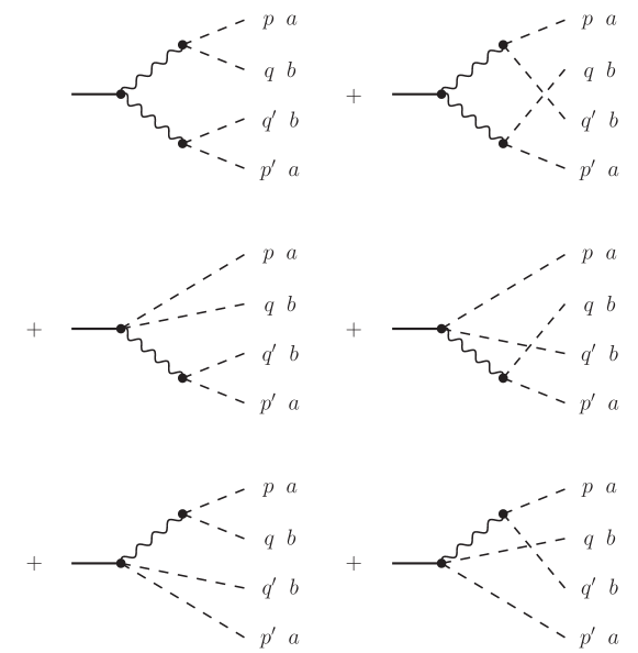
Figure 3: Leading-order glueball decay into four pions, isospin indices $a\not=b$.

To leading order in $1/\alpha^{\prime}$ or equivalently inverse ’t Hooft coupling, the D8 brane action (28) does not give direct couplings of glueballs to more than two pions. These appear only through higher DBI corrections with terms quartic in the field strength $F_{\mu Z}$ as will be discussed further below.

Decays into more than four pions can however proceed through vertices involving vector mesons. The vertices coupling a single glueball to $\pi$ and/or $\rho$ mesons that are obtained from the Yang-Mills part of the D8 brane action (28) arise from terms of the form (dropping derivatives and Lorentz indices)

$$G{\rm Tr}\,(\pi\pi),\quad G{\rm Tr}\,(\rho\rho),\quad G{\rm Tr}\,(\rho[\pi,\pi]),\quad G{\rm Tr}\,([\pi,\rho]^{2}),\quad G{\rm Tr}\,(\rho[\rho,\rho]),\quad G{\rm Tr}\,([\rho,\rho]^{2}).$$ (64)

Only the first three couplings are relevant for the decay of a glueball to $\leq 4$ pions. The corresponding interaction Lagrangians for the exotic and the dilatonic scalar glueball are given explicitly in Appendix B with the coupling constants for the lowest glueball states listed in Table 3 and 4.

The relative width of the decay of a glueball to two pions was found above to be $\Gamma_{G\to\pi\pi}/M\propto\lambda^{-1}N_{c}^{-2}$, parametrically suppressed by a factor $1/N_{c}$ compared to the decay of the $\rho$ meson. For glueballs with mass larger than $2m_{\rho}$, the decay into two $\rho$ mesons is of the same parametric order. However, both the lowest exotic glueball and the lowest dilatonic glueball have mass below the $2\rho$ threshold. In this case at least one $\rho$ meson has to be off-shell, which leads to an additional suppression by a factor $\Gamma_{\rho}/m_{\rho}\propto\lambda^{-1}N_{c}^{-1}$.

Because the vertex coupling a single $\rho$ meson to two pions involves ${\rm Tr}\,(\rho[\pi,\pi])$, the leading-order decay into four pions produces pairs of pions with different isospin index. (The parametrically suppressed decay $G\to 2G\to 4\pi^{0}$ and $G\to G+2\pi^{0}\to 4\pi^{0}$ which only needs the leading Yang-Mills part of the DBI action will be discussed together with the direct decay $G\to 4\pi^{0}$ from higher-order DBI corrections further below.)

IV.2.1 Leading-order decay rate of scalar glueballs to four pions involving $\pi^{\pm}$

The Feynman diagrams for the amplitude of the decay $G_{E,D}\to 2\pi^{a}+2\pi^{b}$ with $a\not=b$ are shown in Fig. 3. Some details of the rather lengthy calculation of the decay rate are given in Appendix C.

Because one internal $\rho$ meson can reach its mass shell, while it has nonnegligible width, we include (following Ref. Hashimoto et al. (2008)) $\Gamma_{\rho}$ in the $\rho$ meson propagator according to $\Delta_{\rho}(r)=1/(r_{0}^{2}-\mathbf{r}^{2}-m_{\rho}^{2}+im_{\rho}\Gamma_{\rho})$ with $\Gamma_{\rho}$ given by (46). This corresponds to a partial summation of higher-order terms in inverse powers of $\lambda N_{c}$. As a crosscheck of our calculations, we have verified that in the limit $\lambda N_{c}\to\infty$ the resulting decay rate agrees with the rate for $G_{E,D}\to\rho\pi\pi$, and in the case of glueballs above the $2\rho$ threshold, with $G\to 2\rho$ (Appendix C.1.2).

Because $m_{\rho}<m_{E,D}<2m_{\rho}$, the leading parametric order of the decay width of $G_{E}$ and $G_{D}$ into four pions is given by the process $G\to\rho\pi\pi$ and reads $\lambda^{-2}N_{c}^{-3}$. Decays through off-shell $\rho$ mesons contribute terms of order $\lambda^{-3}N_{c}^{-4}$.

For $G_{E}$, which is only 10% heavier than a $\rho$ meson, the contribution from one on-shell $\rho$ meson is strongly suppressed by phase space, but the finite width of the $\rho$ meson helps to increase the rate. For $\lambda\approx 16.63$ we find

$$\Gamma_{G_{E}\to 4\pi}/M_{E}\approx 1.33\times 10^{-4}\quad(\lambda\approx 16.63).$$ (65)

For the heavier dilatonic glueball $G_{D}$, the process $G\to\rho\pi\pi$ is more dominant, leading to a significantly larger relative width

$$\Gamma_{G_{D}\to 4\pi}/M_{D}\approx 2.44\times 10^{-3}\quad(\lambda\approx 16.63).$$ (66)

Evidently, the $4\pi$ decay of the lowest holographic glueball state, be it $G_{E}$ or $G_{D}$, is strongly suppressed. Table 6 summarizes these results and also shows them for smaller $\lambda=12.55$. (In Section V we shall consider the extrapolation of these lowest states to the higher masses of experimental glueball candidates in the range predicted by lattice gauge theory.)

IV.2.2 Decay of excited scalar glueballs to two vector mesons

For the excited dilatonic glueball with mass $M_{D^{*}}\approx 2358.4$ MeV, which is above the $2\rho$ threshold, a similar calculation, but with coefficients $d^{*}_{i}$ in place of $d_{i}$ (see Table 4), gives

$$\Gamma_{G_{D}^{*}\to 4\pi}/M_{D^{*}}\approx 0.104\quad(\lambda\approx 16.63).$$ (67)

This result, which involves resummed $\rho$ propagators, is in fact well approximated by the decay rate to two on-shell $\rho$ mesons:

$$\Gamma_{G_{D}^{*}\to 2\rho}/M_{D^{*}}\approx\frac{14.330}{\lambda N_{c}^{2}}\approx 0.096\quad(\lambda\approx 16.63),$$ (68)

which corresponds to the strictly leading-order part of (67) as explained in Appendix C.1.2.

The result (68), divided by its isospin factor of 3, also gives the decay into two isosinglet vector mesons $\omega$, whose mass is only 1% higher than that of the $\rho$ meson.

Since the decay width into two pions given in (59) is much smaller than the width into two vector mesons, the excited dilatonic glueball turns out to decay predominantly into four pions and six pions.

The excited exotic scalar (if we do not discard this mode altogether) is instead dominated by the decay into two pions, which makes this state extremely broad. Calculating also the decay into two vector mesons, we find that the decay into two $\rho$ mesons accounts for only about a third of the total decay into four pions,

$$\Gamma_{G_{E}^{*}\to 2\rho}/M_{E^{*}}\approx\frac{2.078}{\lambda N_{c}^{2}}\approx 0.014\quad(\lambda\approx 16.63).$$ (69)

This means that the decay into four pions is coming largely from the $G_{E}^{*}\rho\pi\pi$ vertex.

In Table 7 the results for the decay widths of the excited exotic and dilatonic scalar glueballs in the Witten-Sakai-Sugimoto model are summarized. While the excited dilatonic scalar glueball has a more moderate decay width compared to the very broad excited exotic scalar, it turns out to be still quite large, around 500 MeV.

	$M$	$\Gamma/M$
$G_{E}\to 4\pi$	855	$1.3\times 10^{-4}$ …$3.0\times 10^{-4}$
$G_{D}\to 4\pi$	1487	$2.4\times 10^{-3}$ …$3.9\times 10^{-3}$
$G_{D}\to 4\pi^{0}$ (NLO-DBI)	1487	$4.0\times 10^{-6}$ …$2.9\times 10^{-5}$
$G_{D}\to G_{E}+2\pi^{0}\to 4\pi^{0}$	1487	$2.6\times 10^{-6}$ …$4.5\times 10^{-6}$
$G_{D}\to G_{D}+2\pi^{0}\to 4\pi^{0}$	1487	$1.9\times 10^{-9}$ …$4.5\times 10^{-9}$

Table 6: Decay widths of lowest exotic and lowest dilatonic scalar glueballs into four (massless) pions divided by glueball mass for $\lambda=16.63\ldots 12.55$.

	$M$	$\Gamma/M$
$G_{E}^{*}\to\{2\pi,2K,2\eta\}$	2168	0.397…0.526
$G_{E}^{*}\to 4\pi$	2168	0.037…0.061
$G_{E}^{*}\to 2\omega\to 6\pi$	2168	0.005…0.006
$G_{E}^{*}\to 2\phi$	2168	0.005…0.006
$G_{E}^{*}$ (total)	2168	0.443…0.599
$G_{D}^{*}\to 4\pi$	2358	0.104…0.142
$G_{D}^{*}\to 2\omega\to 6\pi$	2358	0.032…0.043
$G_{D}^{*}\to 2\phi$	2358	0.032…0.043
$G_{D}^{*}\to\{2\pi,2K,2\eta\}$	2358	0.029…0.039
$G_{D}^{*}$ (total)	2358	0.197…0.267

Table 7: Decay widths of excited scalar glueballs divided by glueball mass for $\lambda=16.63\ldots 12.55$ (chiral limit, with a ratio 3:4:1 for the combined decay into $2\pi,2K,2\eta$).

IV.2.3 Scalar glueball decay to four $\pi^{0}$

The glueball decays into four pions that we have considered above involve pairs of pions with different isospin index. A decay to four $\pi^{0}$ is suppressed by powers of inverse ’t Hooft coupling, because it either has to come from higher-order contributions in the DBI action of the D8 branes (Fig. 4) or has to involve glueball self-interactions and virtual glueballs (Fig. 5).

As shown in Appendix B, the parametric order of the vertex formed by a single glueball and four $\pi^{0}$ turns out to be $\lambda^{-7/2}N_{c}^{-2}$, whereas the amplitude for $G\to 2G\to 4\pi^{0}$ and $G\to G+2\pi^{0}\to 4\pi^{0}$ is proportional to $\lambda^{-3/2}N_{c}^{-3}$. The former thus has stronger suppression in inverse powers of $\lambda$, while the latter is more strongly suppressed with respect to inverse powers of $N_{c}$.

For simplicity, we only consider the dilatonic glueball, since the exotic glueball has a much more complicated interaction Lagrangian. In Appendix B.2.2 the interaction Lagrangian for a dilatonic glueball with four $\pi^{0}$ resulting from the next-to-leading terms of the DBI action has been obtained, and in Appendix B.2.3 the vertex for $G_{D}\to G_{D,E}+2\pi^{0}$. Numerically evaluating the respective decay rates of the dilatonic glueball shows that at finite ’t Hooft coupling and $N_{c}=3$ the dominant decay process comes from the direct coupling of $G_{D}$ to four $\pi^{0}$. For $\lambda\approx 16.63$ we find (see Appendix C.2 for details)

$$\Gamma^{\rm(NLO-DBI)}_{G_{D}\to 4\pi^{0}}/M_{D}\approx 4.02\times 10^{-6}\quad(\lambda\approx 16.63).$$ (70)

The decay through virtual glueballs, while not as strongly suppressed by inverse powers of $\lambda$, is subleading at large $N_{c}$ and is disfavored by phase space. To check whether it might nevertheless be important at $N_{c}=3$ and our range of ’t Hooft coupling, we have evaluated the first diagram in Fig. 5 involving one virtual glueball and found that its contribution is smaller than (70) by several orders of magnitude (see Table 6),

$$\Gamma^{\rm(LO-DBI)}_{G_{D}\to G_{D}+2\pi^{0}\to 4\pi^{0}}/M_{D}\approx 1.94\times 10^{-9}\quad(\lambda\approx 16.63).$$ (71)

If we do not discard the exotic glueball as a physical state (for instance if we were to interpret the latter as holographic dual of a glueball component of the $\sigma$-meson, as speculated at the end of Section IV.1), we should also consider the process $G_{D}\to G_{E}+2\pi^{0}$ which is less suppressed kinematically (but still by $N_{c}^{-1}$). This would be of similar magnitude as the result (70):

$$\Gamma^{\rm(LO-DBI)}_{G_{D}\to G_{E}+2\pi^{0}\to 4\pi^{0}}/M_{D}\approx 2.56\times 10^{-6}\quad(\lambda\approx 16.63).$$ (72)

(As shown in Table 6, at smaller $\lambda$ this contribution is less important compared to the next-to-leading DBI contribution (70).)

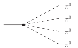
Figure 4: Glueball decay into four $\pi^{0}$ through a vertex from the next-to-leading order terms of the DBI action;

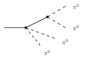
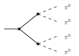
(a) (b)

Figure 5: Glueball decay into four $\pi^{0}$ (a) through terms in the Yang-Mills part of the DBI action that are quadratic in the glueball mode; (b) through a pair of virtual glueballs.

Decays into four $\pi^{0}$ have been seen for the glueball candidate $f_{0}(1500)$ at a level of about an order of magnitude below the general $4\pi$ decay Olive et al. (2014), whereas no such data seem to be available for $f_{0}(1710)$. The smallness of the holographic result (70) however would correspond to a much stronger suppression than the one observed experimentally for $f_{0}(1500)$.

IV.2.4 Tensor glueball decay to two vector mesons

Unless the mass of the lowest tensor glueball is manually adjusted (as we shall consider to do in Section V), only the excited tensor glueball of the Witten model with mass $M_{T^{*}}=M_{D^{*}}\approx 2358.4$ MeV can decay into two $\rho$ or two $\omega$ mesons.

The decay rate involves two sums over the polarizations of the two vector mesons. The average over the polarization of the tensor can again be performed by choosing the particular polarization $\epsilon^{11}=-\epsilon^{22}=1$ and averaging over spatial directions. The rate for two vector mesons with fixed isospin quantum number reads

$$\Gamma=\frac{1}{16\pi M_{T^{*}}}\sqrt{(M_{T^{*}}/2)^{2}-m_{\rho}^{2}}\int\frac{d\Omega}{4\pi}\sum_{\lambda_{1},\lambda_{2}=1}^{3}|\mathcal{M}_{\epsilon_{T}}(\lambda_{1},\lambda_{2})|^{2},$$ (73)

where $\lambda_{1,2}$ are labels for the polarizations of the two vector mesons and $\epsilon_{T}$ refers to the specific tensor polarization. The amplitude $\mathcal{M}_{\epsilon_{T}}(\lambda_{1},\lambda_{2})$ and the final result of the summations and the integration are given in Appendix C.3. With coupling constants $t_{i}^{*}\equiv\sqrt{6}d_{i}^{*}$ and $d_{i}^{*}$ from Table 4, the result for the decay into two $\rho$ mesons is

$$\frac{\Gamma_{T^{*}\to 2\rho\to 4\pi}}{M_{T^{*}}}\approx\frac{21.236}{\lambda N_{c}^{2}}\approx 0.142\quad(\lambda\approx 16.63),$$ (74)

and $1/3$ of that result for the decay $T^{*}\to 2\omega\to 6\pi$. This should be compared to the decay rate into two pions, Eq. (61), which is less than $1/8$ of (74).

As we shall discuss below, a similar pattern arises when the lowest tensor glueball is extrapolated in mass such that it is above the $2\rho$ threshold.

V Extrapolations and comparison with experimental data

When comparing our results for decay rates with experiment, it seems reasonable to do so with the dimensionless ratio $\Gamma/M$ when extrapolating the mass $M$ of the holographic glueball to the mass of the experimental glueball candidates $f_{0}(1500)$ or $f_{0}(1710)$. In the case of decay into two massless pions, Eqs. (57)–(61), this ratio involves two explicit powers of the glueball mass $M$ that cancel the inverse mass scale squared coming from the normalization of the glueball field, Eq. (17) or (23). When extrapolating to higher glueball masses, we thus assume that the normalization of the glueball field scales according to the glueball mass. While this keeps $\Gamma/M$ for two-pion decays unchanged, the decay rates into two vector mesons or four pions are modified and depend in fact strongly on whether the glueball mass is above or below the $2\rho$ threshold.

V.1 Extrapolations for the scalar glueball candidates $f_{0}(1500)$ and $f_{0}(1710)$

The results of such an extrapolation to the experimental masses of the isoscalar mesons $f_{0}(1500)$ or $f_{0}(1710)$ is given in Table 8, where the holographic results of the (chiral) Witten-Sakai-Sugimoto model for the lowest (“exotic”) and the dilatonic $0^{++}$ glueball are compared to the experimental results for the total and the partial decay widths. Here we have generalized our results to $N_{f}=3$ and assumed that pions, kaons and $\eta$ mesons appear in ratios $3:4:1$, respecting SU(3) flavor symmetry.

Explicit masses for quarks would require a modification of the Sakai-Sugimoto model, for example along the lines of Ref. Aharony and Kutasov (2008); Hashimoto et al. (2008); McNees et al. (2008), which we intend to study in future work. This will necessarily modify the coupling of scalar glueballs through contributions that depend on the mass of the pseudo-Goldstone bosons, and this may either increase or decrease the decay amplitudes into the heavier pseudo-Goldstone bosons. A significant enhancement would be in line with the so-called chiral suppression of scalar glueball decays that is suggested by the lattice results of Ref. Sexton et al. (1995) and the analysis of Ref. Chanowitz (2005). (In the dilaton effective theory of Ref. Ellis and Lanik (1985) also an increase of the amplitude for the decay into a pair of heavier pseudo-Goldstone bosons was found, however such that it is approximately canceled by the kinematical suppression from the phase space integral.)

When comparing the extrapolated decay rates of the holographic glueballs with those of the isoscalar mesons $f_{0}(1500)$ or $f_{0}(1710)$ we find that the lowest (exotic) glueball is much too broad to be identified as their dominant glueball component. The dilatonic glueball, however, is sufficiently narrow for this purpose. It leads to a total decay width that is quite close to the experimental width of $f_{0}(1710)$, while being somewhat more strongly below that of $f_{0}(1500)$. With mass equal to that of $f_{0}(1500)$, the dilatonic glueball has significantly smaller width in $2\pi$ decays, and still smaller for decays into four pions, which is the dominant decay mode of the $f_{0}(1500)$.

Regarding the $f_{0}(1710)$, the decay into $2\pi$ is found to be nicely comparable to the experimental value, while the stronger rate into pairs of heavier pseudo-Goldstone bosons remains unaccounted for with our assumption of SU(3) invariance. A significant enhancement of decays into kaons and $\eta$ mesons may however be brought about by mass terms for the latter which inevitably will give additional contributions to the coupling with scalar glueballs.

If our extrapolation of the decay width into $4\pi$ can be trusted, this appears now uncomfortably large considering that the decay of $f_{0}(1710)$ into $4\pi$ has not been observed. It should be noted, however, that the experimental data for the branching ratios of the $f_{0}(1710)$ still have large uncertainties and are not covered by the Particle Data Group Olive et al. (2014). The quoted results are from Refs. Parganlija (2012); Janowski et al. (2014), which assume that decays into $\pi\pi$, $\eta\eta$, and $K\bar{K}$ add up to the total width with negligible contribution from $4\pi$ decays.

Our extrapolations also predict decays into two $\omega$ mesons at a nonnegligible level. According to Olive et al. (2014), decays of $f_{0}(1710)$ to two $\omega$ mesons have at least been seen. The Witten-Sakai-Sugimoto model for a (pure) glueball candidate suggests that the rate into four pions should be about twice as large.

decay	$M^{\rm exp}$	$\Gamma/M$ (exp.)	$\Gamma/M[G_{E}({M^{\rm exp}})]$	$\Gamma/M[G_{D}({M^{\rm exp}})]$
$f_{0}(1500)$ (total)	1505	0.072(5)	0.249…0.332	0.027…0.037
$f_{0}(1500)\to 4\pi$	1505	0.036(3)	0.003…0.006	0.003…0.005
$f_{0}(1500)\to 2\pi$	1505	0.025(2)	0.092…0.122	0.009…0.012
$f_{0}(1500)\to 2K$	1505	0.006(1)	0.123…0.163	0.012…0.016
$f_{0}(1500)\to 2\eta$	1505	0.004(1)	0.031…0.041	0.003…0.004
$f_{0}(1710)$ (total)	1722	0.078(4)	0.252…0.336	0.059…0.076
$f_{0}(1710)\to 2K$	1722	* $\left\{0.041(20)\atop 0.047(17)\right.$	0.123…0.163	0.012…0.016
$f_{0}(1710)\to 2\eta$	1722	* $\left\{0.020(10)\atop 0.022(11)\right.$	0.031…0.041	0.003…0.004
$f_{0}(1710)\to 2\pi$	1722	* $\left\{0.017(4)\atop 0.009(2)\right.$	0.092…0.122	0.009…0.012
$f_{0}(1710)\to 4\pi$	1722	?	0.006…0.010	0.024…0.030
$f_{0}(1710)\to 2\omega\to 6\pi$	1722	seen	0.00016…0.00021	0.011…0.014

Table 8: Experimental data for the decay rates of the isoscalar mesons $f_{0}(1500)$ and $f_{0}(1710)$ juxtaposed to the holographic results for the various decay channels of the lowest (exotic) glueball ($G_{E}$) and predominantly dilatonic glueball ($G_{D}$) with mass $m_{E,D}$ artificially raised to the respective experimental values (still in the chiral limit, i.e. with massless pions, kaons, and $\eta$) and ’t Hooft coupling varied from 16.63 to 12.55. Experimental data are from Ref. Olive et al. (2014) except for those marked by a star, which are from Ref. Parganlija (2012) where the total width of $f_{0}(1710)$ was split under the assumption of a negligible branching ratio to four pions, using data from BES Ablikim et al. (2006) (upper entry) and WA102 Barberis et al. (1999) (lower entry), respectively. (Holographic predictions that are substantially increased due to the manually adjusted glueball mass are rendered in italics.)

In this context it is worth mentioning that there are still many open questions surrounding the nature of $f_{0}(1710)$ Klempt and Zaitsev (2007). For example, some authors have argued that the nearby resonance Ablikim et al. (2005) $f_{0}(1790)$, which is not yet covered by the Particle Data Group, should be combined with $f_{0}(1710)$ into one object $f_{0}(1760)$, for which Ref. Anisovich and Sarantsev (2003) was able to fit disparate decay patterns, with and without significant decay into four pions.

V.2 Extrapolations for the tensor glueball

In the Witten model, with $M_{\rm KK}=949$ MeV, the mass of the tensor glueball equals the mass of the dilatonic scalar glueball, and the tensor glueball has roughly similar decay rates into two and four pions. The rate into two pions practically exhausts the decays into pions, and has been calculated above in Eq. (60). The lowest tensor glueball thus turns out to be a rather narrow state, however this is due to the fact that it stays below the $2\rho$ threshold.

Indeed, the situation is markedly different for the excited tensor glueball $T^{*}$. Its mass equals that of the excited dilatonic glueball, and because this is above the threshold for two $\rho$ mesons, there is a significant contribution to four-pion decays, and also from other vector meson decays, as we have seen in Section IV.2.4. Extrapolating the couplings of the lowest tensor glueball to a similarly high mass, 2 or 2.4 GeV (where the latter is roughly the prediction of lattice gauge theory for the lowest tensor mode), equally gives large contributions from decay into two vector mesons, as listed in Table 9. Reassuringly, these results are quite close to those for the unmodified results for $T^{*}$, cp. Eq. (74), so that we consider them as plausible extrapolations to the likely situation of a tensor glueball with mass above 2 GeV.

decay	M	$\Gamma/M[T(M)]$
$T\to 2\pi$	1487	0.013…0.018
$T\to 2K$	1487	0.004…0.006
$T\to 2\eta$	1487	0.0005…0.0007
$T$ (total)	1487	$\approx 0.02\ldots 0.03$
$T\to 2\rho\to 4\pi$	2000	0.135…0.178
$T\to 2K^{*}\to 2(K\pi)$	2000	0.119…0.177
$T\to 2\omega\to 6\pi$	2000	0.045…0.059
$T\to 2\pi$	2000	0.014…0.018
$T\to 2K$	2000	0.010…0.013
$T\to 2\eta$	2000	0.0018…0.0024
$T$ (total)	2000	$\approx 0.32\ldots 0.45$
$T\to 2K^{*}\to 2(K\pi)$	2400	0.173…0.250
$T\to 2\rho\to 4\pi$	2400	0.159…0.211
$T\to 2\omega\to 6\pi$	2400	0.053…0.070
$T\to 2\phi$	2400	0.032…0.051
$T\to 2\pi$	2400	0.014…0.019
$T\to 2K$	2400	0.012…0.016
$T\to 2\eta$	2400	0.0025…0.0034
$T$ (total)	2400	$\approx 0.45\ldots 0.62$

Table 9: Extrapolation of tensor glueball decay for the case of massive pseudo-Goldstone bosons with glueball mass $M=M_{T}=M_{D}$ and when the latter is raised to 2 GeV or the lattice prediction $\sim 2.4\,{\rm GeV}$. The ’t Hooft coupling is again varied from 16.63 to 12.55.

In Table 9 we have also extrapolated to decays into kaons and $\eta$ mesons. In the holographic setup, a tensor glueball presumably does not couple to an explicit mass term of the pseudoscalar mesons, so the effect of the latter should be purely kinematic. The results (55) and (56) imply a pseudoscalar mass dependence of the form $(1-4m_{\pi}^{2}/M_{T}^{2})^{5/2}$. This suppression is such that it overcompensates the ratio 4/3 that favors kaons over pions.

For the decays into vector mesons $K^{*}$ and $\phi$ we have taken into account that their masses are larger than $m_{\rho}$ in the phase space factor, but we have left open the possibility that this also increases the coupling $t_{2}\equiv\sqrt{6}d_{2}$ and merged the two alternatives in the range of results for the corresponding decay rates for tensor glueballs with increased mass.

Adding up the individual contributions, we find a very broad width for a 2.4 GeV tensor glueball, 1.1 to 1.5 GeV, which is much broader than all the $f_{2}$ mesons listed in Olive et al. (2014). With a mass around 2 GeV, the width (600 to 900 MeV) turns out to be larger but perhaps marginally comparable with that of the tensor meson $f_{2}(1950)$, which has $\Gamma=472(18)$ MeV. The latter is indeed occasionally discussed as a candidate for a tensor glueball as it appears to have largely flavor-blind decay modes.

VI Conclusion

Using the Witten-Sakai-Sugimoto model for holographic QCD, which only has one free dimensionless parameter, we have repeated and extended the calculation of glueball decay rates of Ref. Hashimoto et al. (2008), where only the lowest scalar mode was studied.

This lowest mode is associated with an exotic polarization of the gravitational field, involving components in the direction of compactification from a 5-dimensional super-Yang-Mills theory down to nonsupersymmetric Yang-Mills theory. The mass of this lowest (“exotic”) $0^{++}$ mode turns out to be only slightly above the mass of the $\rho$ meson and is therefore much smaller than the mass scale of glueballs found in lattice gauge theory. The background of the Witten model also contains another tower of scalar glueball modes which are predominantly dilatonic and whose lowest mass is about 1.5 GeV, not far from the predictions of lattice simulations.

Besides its very low mass, the lowest (exotic) scalar glueball turns out to have a decay rate that is significantly higher than that of the heavier dilatonic mode, which seems counterintuitive if the latter were to represent an excitation of the former. We are therefore led to the conjecture that the exotic scalar mode should be discarded so that the glueball spectrum begins with the (predominantly) dilatonic mode as lowest glueball. Another, more speculative possibility that we have mentioned in Section IV.1 is that the exotic scalar mode represents a broad glueball component of the $\sigma$-meson in line with the scenario of Ref. Narison (1998, 2006); Kaminski et al. (2009), which features a broad glueball around 1 GeV and a narrower one around 1.5 GeV.

The decay widths of glueballs obtained in the Witten-Sakai-Sugimoto model are parametrically suppressed by a factor of $\lambda^{-1}N_{c}^{-2}$, but the numerical results vary substantially for the different modes and decay channels, and thus do not give a picture of “universal narrowness” despite the large-$N_{c}$ nature of the Witten-Sakai-Sugimoto model.

A very strong parametric suppression is obtained for the decay into $4\pi^{0}$, as already pointed out in Ref. Hashimoto et al. (2008). We have confirmed that also the final numerical value turns out to be very small.

A noteworthy feature of the Witten-Sakai-Sugimoto model is that the value of the gluon condensate is small, close to its standard SVZ value Shifman et al. (1979), whereas phenomenological models which incorporate a scalar glueball through a QCD dilaton field Ellis and Lanik (1985); Janowski et al. (2014) would require very large gluon condensates to admit only narrow glueball states.

We have also extrapolated our results so that they can be compared with experimental data for the scalar glueball candidates $f_{0}(1500)$ or $f_{0}(1710)$. In the case of $f_{0}(1500)$, our results for the decay widths of the dilatonic glueball are significantly below the observed rates for decay into two pions and even more so for the experimentally dominant decay into four pions. In the case of the $f_{0}(1710)$ meson, the decay rate into two pions comes out in nice agreement with available experimental data. The much stronger rate into kaons is not accounted for, but this may be due to the fact that the Witten-Sakai-Sugimoto model is strictly chiral and the mechanism of chiral suppression Sexton et al. (1995); Chanowitz (2005). However our (crude) extrapolation to the mass of $f_{0}(1710)$ predicts also a significant branching ratio into four pions that has not been seen experimentally. [Although in this context it should be noted that the identification of $f_{0}(1710)$ and its separation from the nearby $f_{0}(1790)$ Ablikim et al. (2005) has been a matter of debate Anisovich and Sarantsev (2003); Klempt and Zaitsev (2007)].

Furthermore, we have studied the decay of tensor glueballs, which in the Witten-Sakai-Sugimoto model have a narrow width into two pions and (when the mass is above the $2\rho$ threshold) a large width into four pseudoscalars, such that at best the isoscalar tensor meson $f_{2}(1950)$ appears to be (marginally) compatible with our the holographic result, while heavier tensor glueballs would have to be broader than the tensor mesons so far discussed in the literature.

In the case of the tensor glueball we can already plausibly anticipate the effects of nonzero pseudo-Goldstone masses. In the case of scalar glueballs the situation is less clear and we intend to study this issue in extensions of the Witten-Sakai-Sugimoto model in a future work. This would be particularly interesting in view of the glueball candidate $f_{0}(1710)$ which according to Ref. Janowski et al. (2014) could be a nearly unmixed glueball and which has a ratio Olive et al. (2014) $\Gamma(\pi\pi)/\Gamma(KK)$ that is significantly below the flavor-symmetric value $3/4$.

Since the holographic results pertain only to pure glueballs, it would clearly be most interesting to study mixing of glueballs with $q\bar{q}$ states as this can strongly obscure signatures of glueball content. In the holographic setup, mixing is suppressed by $1/N_{c}$ Hashimoto et al. (2008) and would presumably require more difficult stringy corrections that are not captured by the effective Lagrangian following from the Witten-Sakai-Sugimoto model. Absent those, it might be interesting to consider a more phenomenological approach such as extended linear sigma models Janowski et al. (2014), where holographic results for the glueball-meson interactions could be used as input instead of fitting to experimental data.

Appendix A Ten-dimensional field equations

The Kaluza-Klein reduction of the eleven-dimensional graviton modes yields metric fluctuations pertaining to the four-sphere, i.e. in the components denoted by $g_{\Omega\Omega}$. Omitting these fluctuations as done in Ref. Hashimoto et al. (2008) corresponds to dropping all vertices proportional to $\breve{c}_{i}$ in the interaction Lagrangian (81) of the exotic scalar glueball. To see whether this reduction could be justified, we check if these truncated modes solve the ten-dimensional field equations of type IIA supergravity.

For the Witten-Sakai-Sugimoto model, the relevant terms of the supergravity action are given by Polchinski (1998)

$$S_{\mathrm{IIA}}=\frac{1}{2\kappa_{10}^{2}}\int d^{10}x\sqrt{-g}\mathrm{e}^{-2\Phi}\left(R+4\nabla_{M}\Phi\nabla^{M}\Phi-\frac{1}{2}\mathrm{e}^{2\Phi}|F_{4}|^{2}\right),$$ (75)

where $2\kappa_{10}^{2}=(2\pi)^{7}l_{s}^{8}$ and $F_{4}=dC_{3}$ is the four-form from the R-R sector of the theory, with

$$|F_{4}|^{2}\equiv\frac{1}{4!}F_{ABCD}F^{ABCD}.$$ (76)

Variation of this action with respect to the background metric $g_{MN}$ and the dilaton field $\Phi$ results in

$$R_{MN}-\frac{1}{2}Rg_{MN}+2\nabla_{M}\Phi\nabla_{N}\Phi-\frac{\mathrm{e}^{2\Phi}}{4!}\left(2{F_{M}}^{ABC}F_{NABC}-3!|F_{4}|^{2}\right)=0$$ (77)

and

$$R+4\nabla_{M}\nabla^{M}\Phi-4\nabla_{M}\Phi\nabla^{M}\Phi=0,$$ (78)

respectively.

The solution to these equations that corresponds to the background of the Witten model is given by the metric (7), the dilaton (8) and a nonvanishing R-R four-form field. The latter is fixed by the requirement that the flux through a unit four-sphere is quantized, i.e.

$$\int_{S^{4}}F_{4}=N_{c}\frac{\kappa_{10}}{\sqrt{\alpha^{\prime}\pi}},$$ (79)

where the factor of $N_{c}$ arises from the fact that we are considering a stack of $N_{c}$ D4-branes. The field strength that satisfies this condition is given by $F_{4}=3R_{\mathrm{D4}}g_{s}^{-1}\omega_{4}$, with $\omega_{4}$ denoting the volume form of the unit four-sphere.

With this information, one can linearize the field equations and plug in the solutions both with and without the spherical fluctuations, which is easily done with computer algebra tools. The result is that for both the dilatonic and exotic glueball modes, the field equations are not satisfied unless the fluctuations along the four-sphere are included. This means that in a rigorous top-down approach the vertices corresponding to the coefficients $\breve{c}_{i}$ have to be included in the calculation of decay rates. (For the dilatonic glueball mode, the need to include $g_{\Omega\Omega}$ fluctuations can also be deduced from the explicit 10-dimensional calculations of Ref. Hashimoto and Oz (1999).)

Appendix B Glueball-meson interaction Lagrangians

The effective interaction Lagrangian of glueballs and $q\bar{q}$ mesons is obtained by inserting the 10-dimensional metric fluctuations (IV) into the D8 brane action and integrating over the bulk coordinates. In this section we give the result for the lowest (exotic) scalar glueball, the dilatonic scalar glueball, and the tensor glueball, expanded up to the order needed for the calculation of decay rates of glueballs into two pions and four pions as discussed in the text.

As discussed above, we do so by keeping induced fluctuations in $g_{\Omega\Omega}$. In the D8 brane action (27) the contribution from the dilaton fluctuation $\delta G_{11,11}$ appearing through the factor $\sqrt{g_{S^{4}}}=g_{\Omega\Omega}^{2}$ in $\sqrt{-\tilde{g}}$ is opposite in sign to that from $e^{-\Phi}$ and larger by a factor $4/3$.

Let us also recall that following Ref. Hashimoto et al. (2008) we use the convention

$$\pi=\pi^{a}T^{a},\quad\rho_{\mu}=\rho^{a}_{\mu}T^{a},\qquad{\rm Tr}\,T^{a}T^{b}=\delta^{ab},$$ (80)

so that for $N_{f}=2$ using Pauli matrices we have $T^{a}=\sigma^{a}/\sqrt{2}$ and ${\rm Tr}\,[T^{a},T^{b}]T^{c}=\sqrt{2}i\epsilon^{abc}$, while Ref. Sakai and Sugimoto (2005a, b) have ${\rm Tr}\,T^{a}T^{b}=\frac{1}{2}\delta^{ab}$. The Minkowski metric used in the 3+1-dimensional Lagrangians is $\eta_{\mu\nu}={\rm diag}(-+++)$.

B.1 Lowest scalar mode

The glueball-meson interactions contributing at leading order to the decay of a glueball into two or four pions are given by the terms linear in the glueball field and up to quadratic in $\rho$, maximally trilinear in $\pi,\rho$ in the Yang-Mills part of the DBI action of the D8 branes. In the case of the lowest (exotic) scalar mode, they read

$$\mathcal{L}_{G_{E}} =- {\rm Tr}\,\Biggl{\{}c_{1}\left[\frac{1}{2}\partial_{\mu}\pi\partial_{\nu}\pi\frac{\partial^{\mu}\partial^{\nu}}{M_{E}^{2}}G_{E}+\frac{1}{4}(\partial_{\mu}\pi)^{2}\left(1-\frac{\Box}{M_{E}^{2}}\right)G_{E}\right]$$ (81)

$$+c_{2}\,M_{\rm KK}^{2}\left[\frac{1}{2}\rho_{\mu}\rho_{\nu}\frac{\partial^{\mu}\partial^{\nu}}{M_{E}^{2}}G_{E}+\frac{1}{4}(\rho_{\mu})^{2}\left(1-\frac{\Box}{M_{E}^{2}}\right)G_{E}\right]$$

$$+c_{3}\left[\frac{1}{2}\bar{F}_{\mu\rho}\bar{F}_{\nu}{}^{\rho}\frac{\partial^{\mu}\partial^{\nu}}{M_{E}^{2}}G_{E}-\frac{1}{8}\bar{F}_{\mu\nu}\bar{F}^{\mu\nu}\left(1+\frac{\Box}{M_{E}^{2}}\right)G_{E}\right]$$

$$+c_{4}\frac{3}{2M_{E}^{2}}\rho_{\mu}\bar{F}^{\mu\nu}\partial_{\nu}G_{E}$$

$$+ic_{5}\left[\partial_{\mu}\pi[\pi,\rho_{\nu}]\frac{\partial^{\mu}\partial^{\nu}}{M_{E}^{2}}G_{E}+\frac{1}{2}\partial_{\mu}\pi[\pi,\rho^{\mu}]\left(1-\frac{\Box}{M_{E}^{2}}\right)G_{E}\right]$$

$$+\frac{1}{2}\breve{c}_{1}\partial_{\mu}\pi\partial^{\mu}\pi\,G_{E}+\frac{1}{2}\breve{c}_{2}\,M_{\rm KK}^{2}\rho_{\mu}\rho^{\mu}G_{E}$$

$$+\frac{1}{4}\breve{c}_{3}\bar{F}_{\mu\nu}\bar{F}^{\mu\nu}G_{E}+i\breve{c}_{5}\partial_{\mu}\pi[\pi,\rho^{\mu}]G_{E}\Biggr{\}},$$

where $\bar{F}_{\mu\nu}\equiv\partial_{\mu}\rho_{\nu}-\partial_{\nu}\rho_{\mu}$ without a commutator term $[\rho_{\mu},\rho_{\nu}]$. This agrees with Ref. Hashimoto et al. (2008), whose notations we have adopted, in the part involving $c_{i}$, but Ref. Hashimoto et al. (2008) effectively dropped all terms proportional to $\breve{c}_{i}$ due to the neglect of $\delta g_{\Omega\Omega}$.

The coefficients $c_{i}$ and $\breve{c}_{i}$ are obtained by integrals over the glueball mode function $H_{E}(Z)$, the $\rho$ meson mode function $\psi_{1}(Z)$, and the pion mode function $\phi_{0}(Z)\propto 1/K$, $K\equiv 1+Z^{2}$, according to

$$c_{1} = \int dZ\frac{\bar{H}_{E}}{\pi K},\qquad c_{2}=2\kappa\int dZ\,K(\psi_{1}^{\prime})^{2}\bar{H}_{E},\qquad c_{3}=2\kappa\int dZ\,K^{-1/3}(\psi_{1})^{2}\bar{H}_{E},$$

$$c_{4} = 2\kappa M_{\rm KK}^{2}\int dZ\frac{20ZK}{(5K-2)^{2}}\psi_{1}\psi^{\prime}_{1}H_{E},\qquad c_{5}=\int dZ\frac{\psi_{1}\bar{H}_{E}}{\pi K},$$

$$\breve{c}_{1} = \int dZ\frac{H_{E}}{4\pi K},\qquad\breve{c}_{2}=\frac{1}{2}\kappa\int dZ\,K(\psi_{1}^{\prime})^{2}H_{E},$$

$$\qquad\breve{c}_{3} = \frac{1}{2}\kappa\int dZ\,K^{-1/3}(\psi_{1})^{2}H_{E},\qquad\breve{c}_{5}=\int dZ\frac{\psi_{1}H_{E}}{4\pi K},$$ (82)

where the integral over $Z$ is from $-\infty$ to $+\infty$ and where following Ref. Hashimoto et al. (2008) we have introduced

$$\bar{H}_{E}(Z)\equiv\left[\frac{1}{4}+\frac{3}{5K-2}\right]H_{E}(Z).$$ (83)

The corresponding coefficients for the excited mode $G_{E}^{*}$ are obtained by replacing the lowest mode function $H_{E}(Z)$ by the next highest eigenfunction.

The numerical results for the coefficients $c_{i}$, $\breve{c}_{i}$ for the lowest mode as well as for $c_{1}^{*}$ and $\breve{c}_{1}^{*}$ for $G_{E}^{*}$ are given in Table 3.

B.2 Dilatonic and tensor mode

B.2.1 Glueball-meson interactions contributing to leading order decays

Restricting ourselves again to glueball -meson interactions contributing to leading order decays to two and four pions, the interaction Lagrangian linear in $G_{D}$ or $T$, up to quadratic in $\rho$, and maximally trilinear in $\pi,\rho$ reads, for the dilatonic mode,

$$\mathcal{L}_{G_{D}} = {\rm Tr}\,\Biggl{\{}d_{1}\frac{1}{2}\partial_{\mu}\pi\partial_{\nu}\pi\left(\eta^{\mu\nu}-\frac{\partial^{\mu}\partial^{\nu}}{\Box}\right)G_{D}+d_{2}M_{\rm KK}^{2}\frac{1}{2}\rho_{\mu}\rho_{\nu}\left(\eta^{\mu\nu}-\frac{\partial^{\mu}\partial^{\nu}}{\Box}\right)G_{D}$$ (84)

$$+d_{3}\frac{1}{2}\bar{F}_{\mu\rho}\bar{F}_{\nu}{}^{\rho}\left(\eta^{\mu\nu}-\frac{\partial^{\mu}\partial^{\nu}}{\Box}\right)G_{D}+id_{5}\partial_{\mu}\pi[\pi,\rho_{\nu}]\left(\eta^{\mu\nu}-\frac{\partial^{\mu}\partial^{\nu}}{\Box}\right)G_{D}\Biggr{\}}$$

with coefficients

$$d_{1} = \int dZ\frac{H_{D}}{\pi K},\qquad d_{2}=2\kappa\int dZ\,K(\psi_{1}^{\prime})^{2}H_{D},$$

$$\qquad d_{3} = 2\kappa\int dZ\,K^{-1/3}(\psi_{1})^{2}H_{D},\qquad d_{5}=\int dZ\frac{\psi_{1}H_{D}}{\pi K},$$ (85)

and for the tensor glueball

$$\mathcal{L}_{T} = {\rm Tr}\,\biggl{\{}\frac{1}{2}t_{1}\,\partial_{\mu}\pi\partial_{\nu}\pi\,T^{\mu\nu}+\frac{1}{2}t_{2}\,M_{\rm KK}^{2}\rho_{\mu}\rho_{\nu}\,T^{\mu\nu}$$ (86)

$$\qquad+\frac{1}{2}t_{3}\,\bar{F}_{\mu\rho}\bar{F}_{\nu}{}^{\rho}\,T^{\mu\nu}+it_{5}\,\partial_{\mu}\pi[\pi,\rho_{\nu}]\,T^{\mu\nu}\biggr{\}}$$

with $t_{i}$ defined in analogy to (B.2.1). Because of $H_{T}\propto H_{D}$ with the normalization conditions (23), we simply have $t_{i}=\sqrt{6}d_{i}$.

The numerical results for $d_{i}$ and the corresponding coefficients $d_{i}^{*}$ for the next-highest dilatonic scalar are given in Table 4.

B.2.2 $G_{D}$-4$\pi^{0}$ vertex from next-to-leading order DBI action

A direct coupling of glueball modes to more than two pions appears only at higher orders of the DBI action of the D8 branes. For the coupling to four $\pi^{0}\equiv\pi^{3}$ we need to expand up to quartic terms in $F^{3}_{\nu Z}$. The action, restricted to $F^{3}_{\nu Z}$, reads

$$S=T_{\rm D8}(2\pi\alpha^{\prime})^{2}\int d^{9}xe^{-\Phi}\sqrt{-\tilde{g}}\left\{-\frac{1}{2}g^{ZZ}g^{\mu\nu}F^{3}_{\mu Z}F^{3}_{\nu Z}+\frac{(2\pi\alpha^{\prime})^{2}}{8}\left[g^{ZZ}g^{\mu\nu}F^{3}_{\mu Z}F^{3}_{\nu Z}\right]^{2}\right\}.$$ (87)

Inserting the metric fluctuations corresponding to the dilatonic glueball and dropping terms that vanish on the mass shell of the glueball gives

$$\mathcal{L}^{G_{D}\to 4\pi^{0}}=3d_{1}^{\prime}\left[(\partial_{\mu}\pi^{0})^{2}\right]^{2}G_{D}-2d_{1}^{\prime}(\partial_{\rho}\pi^{0})^{2}(\partial_{\mu}\pi^{0})(\partial_{\nu}\pi^{0})\left(\eta^{\mu\nu}-\frac{\partial^{\mu}\partial^{\nu}}{M_{D}^{2}}\right)G_{D}$$ (88)

with

$$d_{1}^{\prime}=\frac{3^{9}\pi^{3}}{8\lambda^{3}N_{c}M_{\rm KK}^{4}}\int dZ\,H_{D}K^{-8/3}\approx 2.513\cdot 10^{6}\,\lambda^{-\frac{7}{2}}\,N_{c}^{-2}M_{\rm KK}^{-5}.$$ (89)

B.2.3 Two-glueball-two-$\pi$ vertices

The leading (Yang-Mills) part of the DBI action also contains nonlinear terms with respect to the metric fluctuations dual to glueballs, which have to be considered for the glueball decays in four $\pi^{0}$, which vanish at leading order. Expanding the bilinear term in $\pi$ to second order in the dilatonic mode $G_{D}$ yields

$$\mathcal{L}^{G_{D}G_{D}\pi\pi}=\frac{d_{1}^{DD}}{2}{\rm Tr}\,\biggl{[} 3(\partial_{\mu}\pi)^{2}G_{D}^{2}$$ (90)

$$-\partial_{\mu}\pi\partial_{\nu}\pi\,\eta_{\rho\sigma}\left(\eta^{\mu\rho}-\frac{\partial^{\mu}\partial^{\rho}}{\Box}\right)G_{D}\left(\eta^{\sigma\nu}-\frac{\partial^{\sigma}\partial^{\nu}}{\Box}\right)G_{D}\biggr{]}$$

with

$$d_{1}^{DD}=\int dZ\frac{H_{D}^{2}}{\pi K}=399.04\ldots\lambda^{-1}N_{c}^{-2}M_{\rm KK}^{-2}.$$ (91)

In Eq. (72) we have considered for completeness also the decay through the lowest exotic scalar glueball. For this process the relevant terms in the interaction Lagrangian turn out to be

$$\mathcal{L}^{G_{D}G_{E}\pi^{0}\pi^{0}} = c_{1}^{DE}{\rm Tr}\,\biggl{[}\partial_{\mu}\pi\partial^{\nu}\pi\left(\frac{\partial^{\mu}\partial^{\sigma}}{M_{E}^{2}}G_{E}\right)\left(\eta_{\sigma\nu}-\frac{\partial_{\sigma}\partial_{\nu}}{\Box}\right)G_{D}$$ (92)

$$\qquad\quad-\frac{1}{4}\partial_{\mu}\pi\partial^{\mu}\pi\left(\frac{\partial^{\rho}\partial^{\sigma}}{M_{E}^{2}}G_{E}\right)\left(\eta_{\sigma\rho}-\frac{\partial_{\sigma}\partial_{\rho}}{\Box}\right)G_{D}\biggr{]}$$

with

$$c_{1}^{DE}=\int dZ\frac{H_{D}\bar{H}_{E}}{\pi K}=1653.9\ldots\lambda^{-1}N_{c}^{-2}M_{\rm KK}^{-2}.$$ (93)

Appendix C Four-pion decay amplitudes and phase space integrals

C.1 Decay of scalar glueballs into 4 massless pions involving $\pi^{\pm}$

The leading-order decay amplitude of a glueball into four pions involves two pairs of pions with different isospin index (thus excluding the case of four $\pi^{0}$’s). If $\mathcal{M}$ is the amplitude for $G\to 2\pi^{a}2\pi^{b}$ with fixed $a\not=b$, the total decay rate of a glueball into 4 pions is given by

$$\Gamma_{G\to 4\pi}=\frac{3}{4}\times\frac{1}{2M}\int d{\rm LIPS}_{4}(M)|\mathcal{M}|^{2},$$ (94)

where the factor $\frac{3}{4}$ is due to a factor of 3 for the three different pairs $a,b$ possible, and $\frac{1}{4}$ is the symmetry factor for two pairs of identical particles.

For the decay of a particle at rest with mass $M$ into $n$ particles we have

$$d{\rm LIPS}_{n}(M)=(2\pi)^{4}\delta^{4}\left(M\delta^{\mu}_{0}-\sum_{A=1}^{n}p_{A}^{\mu}\right)\prod_{B=1}^{n}\frac{d^{3}p_{B}}{(2\pi)^{3}2p_{B}^{0}}.$$ (95)

Useful details of how to organize the integration over the final momenta are given in Ref. Hashimoto et al. (2008). As a test of the numerical procedure for implementing these integrations we have used that for massless final states the phase space integral with $\mathcal{M}\equiv 1$ can be done analytically with the result Byckling and Kajantie (1971)

$$\int d{\rm LIPS}_{n}(M)=\frac{M^{2n-4}}{2(4\pi)^{2n-3}\Gamma(n)\Gamma(n-1)}.$$ (96)

C.1.1 Four-pion decay amplitude for the dilatonic glueball

Because the lowest glueball corresponding to an “exotic” polarization of the metric fluctuations has a rather lengthy interaction Lagrangian and because we arrived at the conjecture that the next-higher scalar (predominantly dilatonic) mode should be interpreted as the lowest scalar glueball of QCD, we shall give the decay amplitude into 4 pions explicitly only for the latter. Denoting the final pion four-momenta in $G_{D}\to 2\pi^{a}2\pi^{b}$ by $p,p^{\prime},q,q^{\prime}$ (see Fig. 3) and defining

$$a^{\mu}=q^{\mu}-p^{\mu},\quad b^{\mu}=q^{\prime\mu}-p^{\prime\mu},\quad r^{\mu}=p^{\prime\mu}+q^{\prime\mu},\quad s^{\mu}=p^{\mu}+q^{\mu},\quad r^{0}+s^{0}=M_{D},$$ (97)

we find

$$i\mathcal{M} = \sqrt{2}g_{\rho\pi\pi}\left(\Delta_{\rho}(r)+\Delta_{\rho}(s)\right)d_{5}\,\mathbf{a}\cdot\mathbf{b}$$ (98)

$$+g_{\rho\pi\pi}^{2}\Delta_{\rho}(r)\Delta_{\rho}(s)\biggl{\{}d_{2}M_{\rm KK}^{2}\mathbf{a}\cdot\mathbf{b}$$

$$\qquad+d_{3}\Bigl{[}(a_{0}b_{0}-\mathbf{a}\cdot\mathbf{b})\,\mathbf{r}\cdot\mathbf{s}+\mathbf{a}\cdot\mathbf{b}\,(r_{0}s_{0}-\mathbf{r}\cdot\mathbf{s})$$

$$\qquad\qquad-(a_{0}r_{0}-\mathbf{a}\cdot\mathbf{r})\,\mathbf{b}\cdot\mathbf{s}-(b_{0}s_{0}-\mathbf{b}\cdot\mathbf{s})\,\mathbf{a}\cdot\mathbf{r}\Bigr{]}\biggr{\}}$$

$$+\left(q\leftrightarrow q^{\prime}\right),$$

where $\Delta_{\rho}(r)=1/(r_{0}^{2}-\mathbf{r}^{2}-m_{\rho}^{2}+im_{\rho}\Gamma_{\rho})$ with $\Gamma_{\rho}$ given by (46).

C.1.2 Scalar glueball decay through $\rho\pi\pi$ and $\rho\rho$

The use of a finite width of the $\rho$ meson in the propagator $\Delta_{\rho}$ corresponds to a partial resummation of formally higher order diagrams. This seems to be natural in view of the fact that $\Gamma_{\rho}/m_{\rho}$ is not very small, but it should be kept in mind that e.g. a correction of the residue of the propagator is being dropped.

If the glueball decay were to be treated strictly perturbatively in inverse powers of $\lambda$ and $N_{c}$, one would neglect $\Gamma_{\rho}/m_{\rho}$ as a higher-order contribution and treat the $\rho$ meson as nearly stable. Because to leading order there is no local vertex that would couple a glueball directly to four pions, the leading-order process would then be given by a decay into on-shell $\rho\pi\pi$ with decay width proportional to $\lambda^{-2}N_{c}^{-3}$ as long as the glueball mass is below the $2\rho$ threshold; glueballs with mass larger than $2m_{\rho}$ would have the decay into two $\rho$ mesons as dominant process for the eventual decay into four pions, with partial width proportional to $\lambda^{-1}N_{c}^{-2}$.

We have evaluated the decay rates into $\rho\pi\pi$ (and $\rho\rho$ when $M>2m_{\rho}$) as a cross-check of our results for the decay into four pions, which coincide in the limit of large $\lambda$,

$$\lim_{\lambda\to\infty}\lambda^{2}\,\Gamma_{G\to 4\pi}/M=\lim_{\lambda\to\infty}\lambda^{2}\,\Gamma_{G\to\rho\pi\pi}/M=\gamma_{1}\quad\mbox{for $m_{\rho}<M<2m_{\rho}$},$$ (99)

$$\lim_{\lambda\to\infty}\lambda\,\Gamma_{G\to 4\pi}/M=\lim_{\lambda\to\infty}\lambda\,\Gamma_{G\to 2\rho}/M=\gamma_{2}\quad\mbox{for $M>2m_{\rho}$},$$ (100)

with $\gamma_{1}\approx 22.074N_{c}^{-3}$ for the glueball mode $G_{D}$, and $\gamma_{2}\approx 6.451N_{c}^{-2}$ when its mass is artificially raised to 1722 MeV. Taking these strictly leading-order results as a basis for the decay width into four pions would give somewhat higher numerical values than the above calculation involving a finite $\Gamma_{\rho}$.

For the lowest (exotic) glueball mode, whose mass is not much higher than $m_{\rho}$, we find $\gamma_{1}\approx 0.0030N_{c}^{-3}$ ($\approx 0.00114N_{c}^{-3}$ if the contribution from the $\breve{c}$’s is dropped). Again the results for $\Gamma_{G\to 4\pi}/M$ converge to this limit for $\lambda\to\infty$. However, for $\lambda=16.63$ the effect of resumming $\Gamma_{\rho}$ in the calculation of $\Gamma_{G\to 4\pi}$ is now an increase of the decay width by more than two orders of magnitude compared to the strictly perturbative result that corresponds to a nearly stable $\rho$ meson with negligible width: the latter would give $\Gamma_{G_{E}\to\rho\pi\pi\to 4\pi}/M_{E}\approx 4.0\times 10^{-7}$ compared to $1.3\times 10^{-4}$ from $\Gamma_{G_{E}\to 4\pi}/M_{E}$ with resummed $\rho$ propagators.

The decay amplitudes for $G\to\rho\pi\pi$ are somewhat unwieldy, in particular for the exotic glueball mode. We therefore give details only for the decay of the excited dilatonic glueball into two $\rho$ mesons. (For the analogous decay of the lowest dilatonic glueball when its mass is raised above the $2\rho$ threshold is obtained by replacing $d_{i}^{*}$ by $d_{i}$.)

No phase space integration is involved in this process, but the polarizations of the $\rho$ meson have to be summed over. Denoting the two transverse and the one longitudinal polarization by indices T and L, respectively, the result is

$$\Gamma_{D^{*}\to\rho\rho}/M_{D^{*}}=\frac{3}{32\pi M_{D^{*}}^{3}}\sqrt{M_{D^{*}}^{2}-4m_{\rho}^{2}}\left(|\mathcal{M}_{L}|^{2}+2|\mathcal{M}_{T}|^{2}\right),$$ (101)

with

$$|\mathcal{M}_{L}|=\left|d_{2}^{*}M_{\rm KK}^{2}\frac{M_{D^{*}}^{2}}{4m_{\rho}^{2}}+d_{3}^{*}m_{\rho}^{2}\right|,\quad|\mathcal{M}_{T}|=\left|d_{2}^{*}M_{\rm KK}^{2}+d_{3}^{*}\left(\frac{3}{4}M_{D^{*}}^{2}-2m_{\rho}^{2}\right)\right|.$$ (102)

Decays into two $\omega$ mesons, whose mass equals the $\rho$ meson mass in the Sakai-Sugimoto model (in the real world it is only 1% heavier), is given by the same expression with the overall isospin multiplicity factor $3$ omitted. (For the excited dilatonic glueball, also decay into two $\phi$ mesons becomes relevant, though not for the lowest dilatonic glueball when its mass is raised to one of the glueball candidates as the latter are all below the $2\phi$ threshold.)

C.2 Decay of dilatonic glueball into 4 massless $\pi^{0}$

With $\mathcal{M}$ the amplitude for $G_{D}\to 4\pi^{0}$, the total decay rate is given by

$$\Gamma_{G_{D}\to 4\pi^{0}}=\frac{1}{24}\times\frac{1}{2M}\int d{\rm LIPS}_{4}(M)|\mathcal{M}|^{2}.$$ (103)

The dominant contribution is provided by (88), which leads to

$$\mathcal{M}/(8id_{1}^{\prime}) = 3\left[p\cdot q\,p^{\prime}\cdot q^{\prime}+p\cdot p^{\prime}\,q\cdot q^{\prime}+p\cdot q^{\prime}\,q\cdot p^{\prime}\right]$$ (104)

$$-p\cdot q\,\mathbf{p}^{\prime}\cdot\mathbf{q}^{\prime}-\mathbf{p}\cdot\mathbf{q}\,p^{\prime}\cdot q^{\prime}-p\cdot p^{\prime}\,\mathbf{q}\cdot\mathbf{q}^{\prime}$$

$$-\mathbf{p}\cdot\mathbf{p}^{\prime}\,q\cdot q^{\prime}-p\cdot q^{\prime}\,\mathbf{q}\cdot\mathbf{p}^{\prime}-\mathbf{p}\cdot\mathbf{q}^{\prime}\,q\cdot p^{\prime}.$$

C.3 Decay of tensor glueball into two vector mesons

Unless one adjusts its mass parameter, only the excited tensor mode is above the $2\rho$ threshold. The interaction Lagrangian (86) with $t_{i}$ replaced by $t_{i}^{*}$ determines the amplitude in Eq. (73) for a specific tensor polarization $\epsilon_{T}^{\mu\nu}$ and two $\rho$ mesons with momenta $p,q$ and polarizations $\epsilon^{\mu}(p,\lambda_{1}),\epsilon^{\nu}(q,\lambda_{2})$ as

$$\mathcal{M}_{\epsilon_{T}}(\lambda_{1},\lambda_{2}) = \epsilon_{\mu}(p,\lambda_{1})\epsilon_{\nu}(q,\lambda_{2})\Bigl{[}t^{*}_{2}M_{\rm KK}^{2}\epsilon_{T}^{\mu\nu}$$ (105)

$$\quad-t_{3}^{*}\left(p\cdot\epsilon_{T}\cdot q\,\eta^{\mu\nu}+p\cdot q\,\epsilon_{T}^{\mu\nu}-p^{\nu}\epsilon_{T}^{\mu\rho}q_{\rho}-q^{\mu}\epsilon_{T}^{\nu\rho}p_{\rho}\right)\Bigr{]}.$$

With $p^{0}=q^{0}=M/2$, $\mathbf{p}=-\mathbf{q}$, and $\mathbf{p}^{2}=(M/2)^{2}-m_{\rho}^{2}$, the result of the summation over the polarizations $\lambda_{1}$, $\lambda_{2}$ and the integration over spatial directions reads

$$\int\frac{d\Omega}{4\pi}\sum_{\lambda_{1},\lambda_{2}=1}^{3}|\mathcal{M}_{\epsilon_{T}}(\lambda_{1},\lambda_{2})|^{2} = 2(t_{2}^{*}M_{\rm KK}^{2}/m_{\rho}^{2})^{2}\left(\frac{2}{15}(\mathbf{p}^{2})^{2}+\frac{2}{3}m_{\rho}^{2}\,\mathbf{p}^{2}+m_{\rho}^{4}\right)$$ (106)

$$+4t_{2}^{*}t_{3}^{*}M_{\rm KK}^{2}\left(\frac{4}{3}\mathbf{p}^{2}+m_{\rho}^{2}\right)$$

$$+2t_{3}^{*2}\left(\frac{8}{15}(\mathbf{p}^{2})^{2}+2m_{\rho}^{2}\,\mathbf{p}^{2}+m_{\rho}^{4}\right),$$

with $t_{i}^{*}\equiv\sqrt{6}d_{i}^{*}$ and $d_{i}^{*}$ given in Table 4.

References

- Fritzsch and Gell-Mann (1972) H. Fritzsch and M. Gell-Mann, “Current algebra: Quarks and what else?”, eConf C720906V2 (1972) 135–165, arXiv:hep-ph/0208010.
- Fritzsch and Minkowski (1975) H. Fritzsch and P. Minkowski, “ Resonances, Gluons and the Zweig Rule”, Nuovo Cim. A30 (1975) 393.
- Jaffe and Johnson (1976) R. Jaffe and K. Johnson, “Unconventional States of Confined Quarks and Gluons”, Phys.Lett. B60 (1976) 201.
- Morningstar and Peardon (1999) C. J. Morningstar and M. J. Peardon, “The Glueball spectrum from an anisotropic lattice study”, Phys.Rev. D60 (1999) 034509, arXiv:hep-lat/9901004.
- Chen et al. (2006) Y. Chen, A. Alexandru, S. Dong, T. Draper, I. Horvath, et al., “Glueball spectrum and matrix elements on anisotropic lattices”, Phys.Rev. D73 (2006) 014516, arXiv:hep-lat/0510074.
- Loan et al. (2006) M. Loan, X.-Q. Luo, and Z.-H. Luo, “Monte Carlo study of glueball masses in the Hamiltonian limit of SU(3) lattice gauge theory”, Int.J.Mod.Phys. A21 (2006) 2905–2936, arXiv:hep-lat/0503038.
- Gregory et al. (2012) E. Gregory, A. Irving, B. Lucini, C. McNeile, A. Rago, et al., “Towards the glueball spectrum from unquenched lattice QCD”, JHEP 1210 (2012) 170, arXiv:1208.1858.
- Bugg (2004) D. Bugg, “Four sorts of meson”, Phys.Rept. 397 (2004) 257–358, arXiv:hep-ex/0412045.
- Klempt and Zaitsev (2007) E. Klempt and A. Zaitsev, “Glueballs, Hybrids, Multiquarks. Experimental facts versus QCD inspired concepts”, Phys.Rept. 454 (2007) 1–202, arXiv:0708.4016.
- Crede and Meyer (2009) V. Crede and C. Meyer, “The Experimental Status of Glueballs”, Prog.Part.Nucl.Phys. 63 (2009) 74–116, arXiv:0812.0600.
- Ochs (2013) W. Ochs, “The Status of Glueballs”, J.Phys. G40 (2013) 043001, arXiv:1301.5183.
- Lutz et al. (2009) M. Lutz et al., “Physics Performance Report for PANDA: Strong Interaction Studies with Antiprotons”, arXiv:0903.3905.
- Wiedner (2011) U. Wiedner, “Future Prospects for Hadron Physics at PANDA”, Prog.Part.Nucl.Phys. 66 (2011) 477–518, arXiv:1104.3961.
- Olive et al. (2014) K. Olive et al., “Review of Particle Physics”, Chin.Phys. C38 (2014) 090001.
- Amsler and Close (1996) C. Amsler and F. E. Close, “Is a scalar glueball?”, Phys.Rev. D53 (1996) 295–311, arXiv:hep-ph/9507326.
- Lee and Weingarten (1999) W.-J. Lee and D. Weingarten, “Scalar quarkonium masses and mixing with the lightest scalar glueball”, Phys.Rev. D61 (1999) 014015, arXiv:hep-lat/9910008.
- Close and Kirk (2001) F. E. Close and A. Kirk, “Scalar glueball mixing above 1 GeV and implications for lattice QCD”, Eur.Phys.J. C21 (2001) 531–543, arXiv:hep-ph/0103173.
- Amsler and Törnqvist (2004) C. Amsler and N. Törnqvist, “Mesons beyond the naive quark model”, Phys.Rept. 389 (2004) 61–117.
- Close and Zhao (2005) F. E. Close and Q. Zhao, “Production of , , and in hadronic decays”, Phys.Rev. D71 (2005) 094022, arXiv:hep-ph/0504043.
- Giacosa et al. (2005) F. Giacosa, T. Gutsche, V. Lyubovitskij, and A. Faessler, “Scalar nonet quarkonia and the scalar glueball: Mixing and decays in an effective chiral approach”, Phys.Rev. D72 (2005) 094006, arXiv:hep-ph/0509247.
- Albaladejo and Oller (2008) M. Albaladejo and J. Oller, “Identification of a Scalar Glueball”, Phys.Rev.Lett. 101 (2008) 252002, arXiv:0801.4929.
- Mathieu et al. (2009) V. Mathieu, N. Kochelev, and V. Vento, “The Physics of Glueballs”, Int.J.Mod.Phys. E18 (2009) 1–49, arXiv:0810.4453.
- Janowski et al. (2011) S. Janowski, D. Parganlija, F. Giacosa, and D. H. Rischke, “The Glueball in a Chiral Linear Sigma Model with Vector Mesons”, Phys.Rev. D84 (2011) 054007, arXiv:1103.3238.
- Janowski et al. (2014) S. Janowski, F. Giacosa, and D. H. Rischke, “Is a glueball?”, Phys.Rev. D90 (2014) 114005, arXiv:1408.4921.
- Narison (1998) S. Narison, “Masses, decays and mixings of gluonia in QCD”, Nucl.Phys. B509 (1998) 312–356, arXiv:hep-ph/9612457.
- Minkowski and Ochs (1999) P. Minkowski and W. Ochs, “Identification of the glueballs and the scalar meson nonet of lowest mass”, Eur.Phys.J. C9 (1999) 283–312, arXiv:hep-ph/9811518.
- Minkowski and Ochs (2003) P. Minkowski and W. Ochs, “The Glueball among the light scalar mesons”, Nucl.Phys.Proc.Suppl. 121 (2003) 123–126, arXiv:hep-ph/0209225.
- Ochs (2007) W. Ochs, “Scalar mesons: In search of the lightest glueball”, Nucl.Phys.Proc.Suppl. 174 (2007) 146–150, arXiv:hep-ph/0609207.
- Burakovsky and Page (2000) L. Burakovsky and P. R. Page, “Tensor glueball meson mixing phenomenology”, Eur.Phys.J. C12 (2000) 489–498, arXiv:hep-ph/9906282.
- Cotanch and Williams (2005) S. R. Cotanch and R. A. Williams, “Tensor glueball photoproduction and decay”, Phys.Lett. B621 (2005) 269–275, arXiv:nucl-th/0505074.
- Anisovich (2004) V. Anisovich, “Systematization of tensor mesons and the determination of the glueball”, JETP Lett. 80 (2004) 715–720, arXiv:hep-ph/0412093.
- Anisovich et al. (2005) V. Anisovich, M. Matveev, J. Nyiri, and A. Sarantsev, “Sector of the mesons: Observation of the tensor glueball”, Int.J.Mod.Phys. A20 (2005) 6327–6364, arXiv:hep-ph/0506133.
- Giacosa et al. (2005) F. Giacosa, T. Gutsche, V. Lyubovitskij, and A. Faessler, “Decays of tensor mesons and the tensor glueball in an effective field approach”, Phys.Rev. D72 (2005) 114021, arXiv:hep-ph/0511171.
- Maldacena (1999) J. M. Maldacena, “The Large N limit of superconformal field theories and supergravity”, Int.J.Theor.Phys. 38 (1999) 1113–1133, arXiv:hep-th/9711200.
- Aharony et al. (2000) O. Aharony, S. S. Gubser, J. M. Maldacena, H. Ooguri, and Y. Oz, “Large N field theories, string theory and gravity”, Phys.Rept. 323 (2000) 183–386, arXiv:hep-th/9905111.
- Witten (1998) E. Witten, “Anti-de Sitter space, thermal phase transition, and confinement in gauge theories”, Adv.Theor.Math.Phys. 2 (1998) 505–532, arXiv:hep-th/9803131.
- Gross and Ooguri (1998) D. J. Gross and H. Ooguri, “Aspects of large N gauge theory dynamics as seen by string theory”, Phys.Rev. D58 (1998) 106002, arXiv:hep-th/9805129.
- Csaki et al. (1999) C. Csaki, H. Ooguri, Y. Oz, and J. Terning, “Glueball mass spectrum from supergravity”, JHEP 9901 (1999) 017, arXiv:hep-th/9806021.
- Hashimoto and Oz (1999) A. Hashimoto and Y. Oz, “Aspects of QCD dynamics from string theory”, Nucl.Phys. B548 (1999) 167–179, arXiv:hep-th/9809106.
- Csaki et al. (1999) C. Csaki, J. Russo, K. Sfetsos, and J. Terning, “Supergravity models for (3+1)-dimensional QCD”, Phys.Rev. D60 (1999) 044001, arXiv:hep-th/9902067.
- Constable and Myers (1999) N. R. Constable and R. C. Myers, “Spin-two glueballs, positive energy theorems and the AdS/CFT correspondence”, JHEP 9910 (1999) 037, arXiv:hep-th/9908175.
- Brower et al. (2000) R. C. Brower, S. D. Mathur, and C.-I. Tan, “Glueball spectrum for QCD from AdS supergravity duality”, Nucl.Phys. B587 (2000) 249–276, arXiv:hep-th/0003115.
- Boschi-Filho and Braga (2004) H. Boschi-Filho and N. R. Braga, “QCD/string holographic mapping and glueball mass spectrum”, Eur.Phys.J. C32 (2004) 529–533, arXiv:hep-th/0209080.
- Colangelo et al. (2007) P. Colangelo, F. De Fazio, F. Jugeau, and S. Nicotri, “On the light glueball spectrum in a holographic description of QCD”, Phys.Lett. B652 (2007) 73–78, arXiv:hep-ph/0703316.
- Forkel (2008) H. Forkel, “Holographic glueball structure”, Phys.Rev. D78 (2008) 025001, arXiv:0711.1179.
- Karch and Katz (2002) A. Karch and E. Katz, “Adding flavor to AdS/CFT”, JHEP 0206 (2002) 043, arXiv:hep-th/0205236.
- Kruczenski et al. (2004) M. Kruczenski, D. Mateos, R. C. Myers, and D. J. Winters, “Towards a holographic dual of large QCD”, JHEP 0405 (2004) 041, arXiv:hep-th/0311270.
- Sakai and Sugimoto (2005a) T. Sakai and S. Sugimoto, “Low energy hadron physics in holographic QCD”, Prog.Theor.Phys. 113 (2005)a 843–882, arXiv:hep-th/0412141.
- Sakai and Sugimoto (2005b) T. Sakai and S. Sugimoto, “More on a holographic dual of QCD”, Prog.Theor.Phys. 114 (2005)b 1083–1118, arXiv:hep-th/0507073.
- Hashimoto et al. (2008) K. Hashimoto, C.-I. Tan, and S. Terashima, “Glueball decay in holographic QCD”, Phys.Rev. D77 (2008) 086001, arXiv:0709.2208.
- Lucini and Panero (2013) B. Lucini and M. Panero, “SU(N) gauge theories at large N”, Phys.Rept. 526 (2013) 93–163, arXiv:1210.4997.
- Ellis and Lanik (1985) J. R. Ellis and J. Lanik, “Is scalar gluonium observable?”, Phys.Lett. B150 (1985) 289.
- Shifman et al. (1979) M. A. Shifman, A. Vainshtein, and V. I. Zakharov, “QCD and Resonance Physics. Sum Rules”, Nucl.Phys. B147 (1979) 385–447.
- Becker et al. (2007) K. Becker, M. Becker, and J. Schwarz, “String theory and M-theory: A modern introduction”, 2007.
- Kanitscheider et al. (2008) I. Kanitscheider, K. Skenderis, and M. Taylor, “Precision holography for non-conformal branes”, JHEP 0809 (2008) 094, arXiv:0807.3324.
- Blaizot et al. (2007) J.-P. Blaizot, E. Iancu, U. Kraemmer, and A. Rebhan, “Hard thermal loops and the entropy of supersymmetric Yang-Mills theories”, JHEP 0706 (2007) 035, arXiv:hep-ph/0611393.
- Elander et al. (2014) D. Elander, A. F. Faedo, C. Hoyos, D. Mateos, and M. Piai, “Multiscale confining dynamics from holographic RG flows”, JHEP 1405 (2014) 003, arXiv:1312.7160.
- Lucini et al. (2010) B. Lucini, A. Rago, and E. Rinaldi, “Glueball masses in the large N limit”, JHEP 1008 (2010) 119, arXiv:1007.3879.
- Burrington et al. (2008) B. A. Burrington, V. S. Kaplunovsky, and J. Sonnenschein, “Localized Backreacted Flavor Branes in Holographic QCD”, JHEP 0802 (2008) 001, arXiv:0708.1234.
- Bigazzi and Cotrone (2014) F. Bigazzi and A. L. Cotrone, “Holographic QCD with Dynamical Flavors”, arXiv:1410.2443.
- Bali et al. (2013) G. S. Bali, F. Bursa, L. Castagnini, S. Collins, L. Del Debbio, et al., “Mesons in large-N QCD”, JHEP 1306 (2013) 071, arXiv:1304.4437.
- Rebhan (2015) A. Rebhan, “The Witten-Sakai-Sugimoto model: A brief review and some recent results”, EPJ Web Conf. 95 (2015) 02005, arXiv:1410.8858.
- Antonyan et al. (2006) E. Antonyan, J. Harvey, S. Jensen, and D. Kutasov, “NJL and QCD from string theory”, arXiv:hep-th/0604017.
- Aharony et al. (2007) O. Aharony, J. Sonnenschein, and S. Yankielowicz, “A Holographic model of deconfinement and chiral symmetry restoration”, Annals Phys. 322 (2007) 1420–1443, arXiv:hep-th/0604161.
- Peeters and Zamaklar (2007) K. Peeters and M. Zamaklar, “The String/gauge theory correspondence in QCD”, Eur.Phys.J.ST 152 (2007) 113–138, arXiv:0708.1502.
- Callebaut et al. (2013) N. Callebaut, D. Dudal, and H. Verschelde, “Holographic rho mesons in an external magnetic field”, JHEP 1303 (2013) 033, arXiv:1105.2217.
- Imoto et al. (2010) T. Imoto, T. Sakai, and S. Sugimoto, “Mesons as Open Strings in a Holographic Dual of QCD”, Prog.Theor.Phys. 124 (2010) 263–284, arXiv:1005.0655.
- Ioffe (2006) B. Ioffe, “QCD at low energies”, Prog.Part.Nucl.Phys. 56 (2006) 232–277, arXiv:hep-ph/0502148.
- Narison (2012) S. Narison, “Gluon Condensates and from QCD-Moments and their ratios to Order and ”, Phys.Lett. B706 (2012) 412–422, arXiv:1105.2922.
- Bali et al. (2014) G. S. Bali, C. Bauer, and A. Pineda, “Model-independent determination of the gluon condensate in four-dimensional SU(3) gauge theory”, Phys.Rev.Lett. 113 (2014) 092001, arXiv:1403.6477.
- Bergman et al. (2007) O. Bergman, S. Seki, and J. Sonnenschein, “Quark mass and condensate in HQCD”, JHEP 0712 (2007) 037, arXiv:0708.2839.
- Aharony and Kutasov (2008) O. Aharony and D. Kutasov, “Holographic Duals of Long Open Strings”, Phys.Rev. D78 (2008) 026005, arXiv:0803.3547.
- Hashimoto et al. (2008) K. Hashimoto, T. Hirayama, F.-L. Lin, and H.-U. Yee, “Quark Mass Deformation of Holographic Massless QCD”, JHEP 0807 (2008) 089, arXiv:0803.4192.
- McNees et al. (2008) R. McNees, R. C. Myers, and A. Sinha, “On quark masses in holographic QCD”, JHEP 0811 (2008) 056, arXiv:0807.5127.
- Narison (2006) S. Narison, “QCD tests of the puzzling scalar mesons”, Phys.Rev. D73 (2006) 114024, arXiv:hep-ph/0512256.
- Mennessier et al. (2008) G. Mennessier, S. Narison, and W. Ochs, “Glueball nature of the from and scatterings”, Phys.Lett. B665 (2008) 205–211, arXiv:0804.4452.
- Kaminski et al. (2009) R. Kaminski, G. Mennessier, and S. Narison, “Gluonium nature of the from its coupling to ”, Phys.Lett. B680 (2009) 148–153, arXiv:0904.2555.
- Parganlija (2012) D. Parganlija, “Quarkonium Phenomenology in Vacuum”, arXiv:1208.0204.
- Ablikim et al. (2006) M. Ablikim, J. Bai, Y. Ban, J. Bian, X. Cai, et al., “Partial wave analyses of and ”, Phys.Lett. B642 (2006) 441–448, arXiv:hep-ex/0603048.
- Barberis et al. (1999) D. Barberis et al., “A Coupled channel analysis of the centrally produced and final states in interactions at 450 GeV/c”, Phys.Lett. B462 (1999) 462–470, arXiv:hep-ex/9907055.
- Sexton et al. (1995) J. Sexton, A. Vaccarino, and D. Weingarten, “Numerical evidence for the observation of a scalar glueball”, Phys.Rev.Lett. 75 (1995) 4563–4566, arXiv:hep-lat/9510022.
- Chanowitz (2005) M. Chanowitz, “Chiral suppression of scalar glueball decay”, Phys.Rev.Lett. 95 (2005) 172001, arXiv:hep-ph/0506125.
- Ablikim et al. (2005) M. Ablikim et al., “Resonances in and ”, Phys.Lett. B607 (2005) 243–253, arXiv:hep-ex/0411001.
- Anisovich and Sarantsev (2003) V. Anisovich and A. Sarantsev, “ matrix analysis of the ()-wave in the mass region below 1900 MeV”, Eur.Phys.J. A16 (2003) 229–258, arXiv:hep-ph/0204328.
- Polchinski (1998) J. Polchinski, “String theory. Vol. 2: Superstring theory and beyond”, 1998.
- Byckling and Kajantie (1971) E. Byckling and K. Kajantie, “Particle Kinematics”, 1971.