A method to discriminate solar and antisolar differential rotation in high-precision light curves

Abstract

Context. Surface differential rotation (DR) is one major ingredient of the magnetic field generation process in the Sun and likely in other stars. The term solar-like differential rotation describes the observation that solar equatorial regions rotate faster than polar ones. The opposite effect of polar regions rotating faster than equatorial ones (termed as antisolar DR) has only been observed in a few stars, although there is evidence from theoretical dynamo models.

Aims. We present a new method to detect the sign of DR (i.e. solar-like or antisolar DR) by analyzing long-term high-precision light curves with the Lomb-Scargle periodogram.

Methods. We compute the Lomb-Scargle periodogram and identify a set of significant periods $P_{k}$, which we associate with active regions located at different latitudes on the the stellar surface. If detectable, the first harmonics ($P_{k}^{\prime}$) of these periods were identified to compute their peak-height-ratios $r_{k}:=h(P_{k}^{\prime})/h(P_{k})$. Spots rotating at lower latitudes generate less sine-shaped light curves, which requires additional power in the harmonics, and results in larger ratios $r_{k}$. Comparing different ratios $r_{k}$ and the associated periods $P_{k}$ yields information about the spot latitudes, and reveals the sign of DR.

Results. We tested our method on different sets of synthetic light curves all exhibiting solar-like DR. The number of cases where our method detects antisolar DR is the false-positive rate of our method. Depending on the set of light curves, the noise level, the required minimum peak separation, and the presence or absence of spot evolution, our method fails to detect the correct sign in at most 20 %. We applied our method to 50 Kepler G stars and found 21–34 stars with solar-like DR and 5–10 stars with antisolar DR, depending on the minimum peak separation.

Conclusions. The method is capable of determining the sign of DR in a statistical way with a rather low false-positive rate. Applying our method to real data might suggest that – within the uncertainties – antisolar DR was detected in 5–10 Kepler stars.

1 Introduction

The differential rotation (DR) of the solar surface (and its interior) is a crucial part of the generation of the Sun’s magnetic field and the solar dynamo. The differential rotation winds up magnetic field lines, which can be considered as frozen in the plasma, transferring an initial poloidal field into a toroidal one. Speaking of solar or solar-like differential rotation in the following we always think of latitudinal-dependent surface rotation rates, with equatorial regions rotating faster than polar ones. This latitudinal shear is usually described by the equation

$$\Omega(\theta)=\Omega_{\rm eq}(1-\alpha\sin^{2}\theta),$$ (1)

where $\Omega_{\rm eq}$ denotes the equatorial angular velocity, $\theta$ the latitude, and $\alpha$ a dimensionless parameter describing the amount of surface shear. The Sun has a relative shear of $\alpha_{\odot}=0.2$. According to eq. 1 DR in stars other than the Sun is usually termed solar-like when $\alpha>0$, whereas the opposite effect, $\alpha<0$, is called antisolar; the case $\alpha=0$ describes rigid (surface) rotation. For other purposes DR might also be expressed in terms of the absolute surface shear $\Delta\Omega=\Omega_{\rm eq}-\Omega_{\rm pole}=\alpha\Omega_{\rm eq}$.

Measuring DR is challenging, because it acts as a subtle perturbation of the mean rotation rate. For stars other than the Sun different techniques have been used. Reiners & Schmitt (2002) applied the Fourier transform method to Doppler broadened spectral lines. Doppler Imaging (Donati & Collier Cameron, 1997) traces active regions located at different latitudes to infer the absolute surface shear $\Delta\Omega$. Furthermore, DR can also be measured from asteroseismology (Gizon & Solanki, 2004; Lund et al., 2014). Classical spot models also supply a measure on DR, with recent studies being, e.g., Lanza et al. (2014); Bonanno et al. (2014). Using the short-term Fourier-transform Vida et al. (2014) provided measurements of activity cycles of fast rotating Kepler stars attributing the observed change in rotation period to DR. Another approach was presented by Reinhold et al. (2013) by measuring different periods in high-precision light curves. This method only yields absolute values of the shear but provides no information of the sign, because the latitudes of the active regions are usually unknown.

Fig. 1 illustrates that it is difficult to tell from the light curve whether the star exhibits solar or antisolar DR. Both light curves were drawn from the same parameters and show an almost identical beating pattern, with the exception that $\alpha$ is positive (negative) in the upper (lower) panel, respectively. Thus, visual inspection of the light curve does not immediately reveal the underlying rotational behavior.

Figure 1: Upper panel: Simulated light curve of a star with two spots and an equator-to-pole shear $\alpha=0.085$ (solar-like DR) according to eq. 1. Lower panel: Same parameters as above but with a negative value of $\alpha=-0.085$ instead (antisolar DR).

Recently, 3D numerical simulations have tabled the question which physical conditions lead to solar-like or antisolar differential rotation, and which parameters determine the transition region (Guerrero et al., 2013; Gastine et al., 2014; Käpylä et al., 2014; Karak et al., 2014). A theoretical explanation for the existence of antisolar DR is provided by Kitchatinov & Rüdiger (2004) favoring the explanation of fast meridional motion. Nevertheless, observations of antisolar DR are sparse and have only been claimed in some K giants so far. Strassmeier et al. (2003) found strong signatures of antisolar DR on the K2-giant HD 31993 supplying the value $\alpha=-0.125\pm 0.05$. Weber et al. (2005) found marginal evidence for antisolar DR in several K giants. Kővári et al. (2007) detected antisolar DR of the K1 giant $\sigma$ Geminorum providing a relative shear of $\alpha\approx-0.022\pm 0.006$. Later studies of the same object approved antisolar DR, almost twice as strong as the earlier value (Kovari et al., 2014). Vida et al. (2007) observed antisolar DR in the K0 giant UZ libræ using cross-correlation of consecutive Doppler images obtained in the years 1998 and 2000, yielding $\alpha\approx-0.03$ and $\alpha\approx-0.004$, respectively. Dikpati & Cally (2011) analyzed the stability of toroidal magnetic fields and differential rotation and found that kG-fields (i.e. activity) are only compatible with small shear if the DR is antisolar. The finding agrees with the small values observed. Furthermore, Ammler-von Eiff & Reiners (2012) applied the Fourier transform method to a sample of more than 110 A–F field stars. For the majority of stars in their sample these authors either found no signature of DR or very small values consistent with rigid rotation. For 10 stars significant DR $(0.10<\alpha<0.50)$ was detected. Five stars in their sample showed signatures which can be explained by antisolar DR. Nevertheless, the authors interpreted the measurements as rigid rotators with cool polar caps.

The goal of this article is to present a new method to measure the sign of DR from high-precision light curves. We compute their Lomb-Scargle periodograms and show how different periods can be associated with higher or lower latitudes using overtone amplitudes. No explicit spot modeling is needed! We explain the method in detail, present results for simulated light curves, and discuss the problems when applying this technique to Kepler data. The paper is organized as follows: In Sect. 2 we motivate the parameter space of the simulated light curves. Section 3 contains a detailed description of the method. The application of the method to simulated and real data is presented in Sect. 4. The last section is dedicated to a detailed discussion of the results.

2 Simulations

In order to test our method we simulated different sets of differentially rotating stars. Each set consists of 100 light curves and was generated by our code MODSTAR (Reinhold & Reiners, 2013). The code creates a spherical surface of a rotating spotted star. Each surface element has a fixed intensity value. Spots are modeled as circular areas with a spot-to-photosphere contrast of 0.67, which roughly corresponds to the solar penumbra-to-photosphere contrast. For simplicity, umbra and penumbra structures of star spots as well as non-circular spot shapes were neglected.

The crucial parameters to describe latitudinal shear are the equatorial rotation period $P_{\rm eq}=2\pi/\Omega_{\rm eq}$, the equator-to-pole shear $\alpha$ , and the spot latitudes (see eq. 1). Further parameters of interest are the number of spots and the stellar inclination angle $i$. All light curves were created using the following parameters, which were chosen at random for each light curve. The stellar inclination ranges from $30^{\circ}<i<80^{\circ}$, the equatorial rotation period from $1<P_{\rm eq}<20$ days, and the equator-to-pole shear covers $0.05<\alpha<0.30$. We emphasize that all simulated stars exhibit a positive $\alpha$, and thus solar-like DR!

The first model set consists of 100 stars with only two spots at fixed latitudes $\theta_{1}=10^{\circ}$ and $\theta_{2}=60^{\circ}$. The second set contains 100 model stars with 10 spots located at random latitudes between $-30^{\circ}<\theta<90^{\circ}$. The number of spots and their latitudes is the only difference between the two sets. The spots can cover the full longitude range $-180^{\circ}<\varphi<180^{\circ}$, with radii between $4^{\circ}<r<6^{\circ}$. For the 10-spot models these radii correspond to a spot coverage of $\sim 1-3$%. Additionally, spots are allowed to overlap without further contrast reduction. Each light curve covers a total length of 1500 days, with a sampling rate of 4 points/day.

The spots in our simple models have infinite lifetimes, i.e., their radii do not change with time. Spot evolution can also be implemented in the models by increasing or decreasing the spot radii. In Sect. 4 we test the robustness of our method under various perturbations, especially probing the effect of spot evolution. Since there are many ways of realizing spot evolution, we chose a simple approach by changing the spot radii when creating the light curves. At the beginning of the simulation the program chooses at random whether all spots should be increased or decreased. Over a course of 30 days, all spot radii are then successively changed by 0.4^∘ in total. Every 30 days, the program chooses again whether the spots should be increased or decreased. Owing to the method it happens that spot radii drop below $0^{\circ}$. In such cases the spots are forced to increase again during the next 30 days period. Both the 30-day interval as well as the amount of 0.4^∘ growth or decay in radii was chosen such that the light curves visually exhibit similar shape to what can be found in Kepler data.

The first model set only contains stars with two spots on their surface. These sets might not be very realistic, but are sufficient to probe the signature of higher and lower latitude spots in the light curve. This set is ideal to present the power of our method, and to focus on the primary goal of detecting the correct sign of $\alpha$. The other parameters were chosen to be comparable with Kepler data. We chose an upper limit of 20 days or the equatorial rotation period, because many Kepler stars exhibit very stable rotation periods in this time regime. Longer periods usually become unstable due to spot evolution, stronger differential rotation, or instrumental effects. From previous simulations we know that DR is hard to detect in stars with small equator-to-pole shear (Reinhold & Reiners, 2013), so a lower limit of $\alpha>0.05$ was imposed. The inclination is limited to $i>30^{\circ}$, because our method tends to fail for lower values. Furthermore, the total length of the light curves in comparable to Kepler’s observing time span.

3 Method

We compute the generalized Lomb-Scargle periodogram (Zechmeister & Kürster, 2009) of the full light curves, identify the 30 highest peaks, and sort them by their peak heights in descending order. The highest-peak period is termed $P_{1}$ and represents the most significant period in the data. To measure the amount of latitudinal DR we search for periods adjacent to $P_{1}$ in the range of $P_{1}\pm 30\,\%$ with peak heights greater than 50. This value represents a lower limit of the significance level of the period in the data, and was chosen after by-eye inspection of several periodograms. The second highest period satisfying the above conditions is termed $P_{2}$, the third highest peak $P_{3}$, and so on.

Ideally these periods belong to certain spot rotation periods, i.e., to spots rotating at certain latitudes. For the 2-spot model we found that this assignment is true for almost all cases (see Sect. 4.1). Unfortunately, for the 10-spot models (Sect. 4.2) this association is not valid anymore, because not every spot is resolved by an individual peak. Furthermore, in real data the number of spots on the surface is unknown, and one has to assign the peaks to spots (or spot groups) on the surface to get a measure of the latitudinal DR. Naturally one would use the highest-peak periods $P_{1}$ and $P_{2}$ to guarantee that these are really present in the data. But no matter which peaks are used to get a measure on DR, they only provide an absolute value of the surface shear, because there is no information about the associated spot latitudes. In the following we show that latitudinal information can be achieved by taking into account the first harmonics (half periods) of the selected periods.

The light curve signature of a single star spot rotating in and out of view depends on its radius, the intensity contrast with its surrounding, the stellar inclination angle, and the spot latitude. In our model we assume circular spot shape and neglect any temperature gradient within the spot. Our method is based on the outcome of the simulations that – for a wide parameter range – lower latitude spots generate less sine-shaped light curves compared to higher latitude spots. As a consequence, additional harmonics of the primary period are required for a proper fit. Since the goodness of a sine fit is equivalent to the peak height in the periodogram, one can achieve information about the spot latitude by comparing the heights of selected peaks and their harmonics. We search the periodogram for the first harmonic of all periods $P_{k},\ k=1,2,...$ satisfying the above conditions, because in some cases the harmonics of $P_{1}$ and $P_{2}$ cannot be detected. If present, the harmonics are termed $P_{k}^{\prime}$ and should lie within 1 % of the half periods $P_{k}/2$, i.e., they should satisfy $0.99P_{k}/2<P_{k}^{\prime}<1.01P_{k}/2$. The corresponding peak heights of the periods $P_{k}$ are termed $h(P_{k})$ and of the harmonics $h(P_{k}^{\prime})$, respectively. For all pairs ($P_{k},P_{k}^{\prime}$) satisfying the above relations we compute the peak-height-ratios (PHR) $r_{k}:=h(P_{k}^{\prime})/h(P_{k})$. Comparing different ratios now reveals information about the spot latitude. The relation $r_{k}>r_{k+1}$ means that the relative power of the harmonic compared to the power of the corresponding period is higher for $k$ than for $k+1$. In this case, we associate the period $P_{k}$ with a lower latitude spot compared to the spot latitude associated with $P_{k+1}$. We define

$$\left.\begin{array}[]{c}\hskip 56.9055ptP_{\rm low}:=P_{k}\\ \hskip 56.9055ptP_{\rm high}:=P_{k+1}\end{array}\right\}\qquad\text{if}\qquad r_{k}>r_{k+1}$$ (2)

and

$$\left.\begin{array}[]{c}\hskip 56.9055ptP_{\rm low}:=P_{k+1}\\ \hskip 56.9055ptP_{\rm high}:=P_{k}\end{array}\right\}\qquad\text{if}\qquad r_{k+1}>r_{k}.$$ (3)

Since we sorted the periods according to their peak heights, we start to compare the PHR with the lowest $k$-value, $k_{\rm min}$, satisfying all conditions, to infer the rotation law. In most cases, $k_{\rm min}=1$ is used if $P_{1}^{\prime}$ is detectable. If $P_{\rm low}<P_{\rm high}$ for $k=k_{\rm min}$ the star exhibits solar-like DR. If the opposite relation is true, antisolar DR is present. Thus, comparing the PHR and the corresponding periods yields the sign of DR!

In some cases contradictory results are returned by comparing the PHR for different $k$-values, e.g., when the comparison for $k=1$ reveals solar-like DR, and for $k=2$ antisolar DR, or vice versa. This happens because the routine matches all peaks in the range of the rotation period to their harmonics, and associates them with spot rotation rates at different latitudes. Because of the fact that not each and every single peak can be associated with a certain spot rotation rate, in some cases the periods are associated with the wrong latitudes. To minimize this effect, we only use the relation for $k=k_{\rm min}$, because $k_{\rm min}$ uses the two highest peaks with detectable harmonics, for comparison.

For the 10-spot models we checked under which conditions a negative sign of DR is returned. To minimize the number of wrong detections we imposed some constraints on the program. For stars with too many individually resolved periods $P_{k}$, we restricted the search to $k\leq 5$. Furthermore, the ratios $r_{k}$ and $r_{k+1}$ must differ by at least 10 %. The largest contribution of wrong detections results from choosing peaks very close to each other, so we forced the program to only match peaks which are separated by at least five points on the frequency grid. Relaxing this condition has a large impact on the number of detection in real data (see Sect. 4.3), and is discussed in Sect. 5.

Figure 2: Upper panel: Light curve of a randomly selected star from the 10-spot models without spot evolution. Lower panel: Periodogram of the above light curve. The peaks of the pairs ($P_{1},P_{1}^{\prime}$) and ($P_{2},P_{2}^{\prime}$) are clearly visible and emphasized by black upside down and normal triangles, respectively.

To illustrate the method Fig. 2 shows the periodogram of a randomly selected light curve from the 10-spot model without spot evolution. In this model the periods and harmonics for $k=1,...,4$ satisfy all conditions and are collected in Table 1. To infer the rotation law the peaks of the pairs ($P_{1},P_{1}^{\prime}$) and ($P_{2},P_{2}^{\prime}$) are selected and emphasized by black upside down and normal triangles, respectively. We detected the periods $P_{1}=15.15$ d, $P_{2}=13.76$ d, $P_{1}^{\prime}=7.61$ d, $P_{2}^{\prime}=6.85$ d, and the ratios $r_{1}=0.026$ and $r_{2}=0.277$. Since $r_{2}>r_{1}$ the period $P_{2}$ belongs to a lower latitude spot (see eq. 3), and the relation $P_{2}<P_{1}$ reveals solar-like DR! The original spot rotation periods $P_{\rm spot}$ of this model lie in the range 13.71 d $<P_{\rm spot}<16.47$ d, showing that the periodogram detects different periods in the right range. Further parameters of the picked model are $i=60.6^{\circ}$ and $\alpha=0.168$.

$k$	1	2	3	4
$P_{k}$	15.15	13.76	14.28	14.56
$P_{k}^{\prime}$	7.61	6.85	7.07	7.25
$r_{k}$	0.026	0.277	0.141	0.085

Table 1: Periods $P_{k}$, harmonics $P_{k}^{\prime}$, and ratios $r_{k}$ for $k=1,...,4$ satisfying all conditions for the model star in Fig. 2.

4 Results

In this section we present the results of the application of our method to the different artificial and real data sets. To quantify the results we provide the distribution of the observed relative differential rotation $\alpha_{\rm obs}$, which we define as

$$\alpha_{\rm obs}:=\frac{P_{\rm high}-P_{\rm low}}{P_{\rm high}},$$ (4)

with the periods $P_{\rm high}$ and $P_{\rm low}$ from eqn. (2) and (3). This quantity automatically provides the false-positive rate of our method, being the number of stars with negative $\alpha_{\rm obs}$ values. Negative values of $\alpha_{\rm obs}$ result from associating certain periods with the wrong latitudes as discussed in Sect. 3. Again, we remind the reader that all simulated stars exhibit $\alpha>0$.

As we will show in the following, the false-positive rate is rather small for unperturbed data. The above sets of light curves are noise-free, the spots do not evolve with time, and – compared to real data – come without gaps or instrumental effects. To test the robustness of our method we include different perturbations in the light curves. We found that spot evolution has the largest effect, so for each set we varied the spot radii with time (see Sect. 2) using the same parameters as in the unperturbed case, and considered different levels of Poisson noise.

To quantify the impact of each effect we compare the distribution of $\alpha_{\rm obs}$ to the distribution of the measurable shear of the model. Therefore, we define $\alpha_{\rm model}:=(P_{\rm max}-P_{\rm min})/P_{\rm max}$, with $P_{\rm max}=\max(P(\theta))$ and $P_{\rm min}=\min(P(\theta))$, being the maximum and minimum periods of the model, respectively. By definition it holds $\alpha_{\rm obs}\leq\alpha_{\rm model}$, because the periods $P_{\rm high}$ and $P_{\rm low}$ do not necessarily belong to the highest and lowest latitude spots, respectively. For each model set we show how well the original spot periods are recovered, directly providing the false-positive rate of our method.

4.1 2-spot models

The distributions of $\alpha_{\rm model}$ and $\alpha_{\rm obs}$ are shown in Fig. 3 in solid black and dashed red, respectively. The upper panel shows the distributions without spot evolution, whereas in the lower panel spot evolution is included in the models. In both panels, the noise level increases from left to right.

For non-evolving spots we find $\alpha_{\rm obs}>0$ in 97 of 100 cases in the noise-free models. For the 3 remaining stars the conditions were not fulfilled, i.e., the false-positive rate is zero! Almost the same result was found when adding 500 ppm Poisson noise to the light curves, with 97 solar-like and 1 antisolar detections. Adding 1000 ppm white noise yields solar-like DR for 85 stars, and no detection for the remaining 15 light curves. Adding even higher noise seems unreasonable, because the periodicity in the light curves visible to the naked eye gets corrupted. Although the main rotation periods are still detectable, their harmonics cannot be identified correctly, because the large noise is interpreted as short periods in the periodograms. Such noisy light curves have not been considered when searching for DR in Kepler data (Reinhold et al., 2013).

We also considered the same models including spot evolution. For the noise-free, the 500 ppm, and the 1000 ppm models we find 94, 90, and 74 solar-like detections, respectively. Only one case of antisolar rotation was detected in the 1000 ppm model. In all cases we find good agreement between the model periods and the recovered values. Furthermore, the false-positive rate is zero for almost all cases supporting the power of the method.

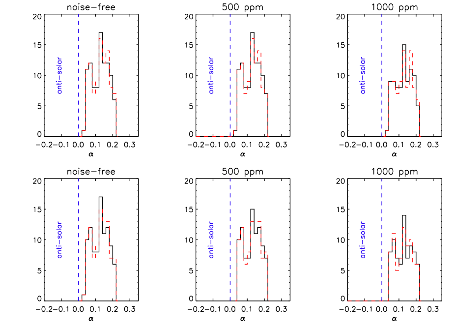
Figure 3: Distributions of $\alpha_{\rm model}$ (solid black) and $\alpha_{\rm obs}$ (dashed red) of the 2-spot model for different noise levels. Upper panel: No spot evolution, Lower panel: Spot evolution included. The dashed blue line indicates $\alpha_{\rm obs}=0$.

4.2 10-spot models

In Fig. 4 we show the distributions of $\alpha_{\rm model}$ and $\alpha_{\rm obs}$ of the 10-spot models in solid black and dashed red, respectively. Again, distributions in the upper panel are without spot evolution, whereas spot evolution is included in the lower panel, and the noise level increases from left to right.

The distributions of $\alpha_{\rm obs}$ look very different to the ones of the 2-spot models, with $\alpha_{\rm obs}$ being much lower than $\alpha_{\rm model}$, on average. The shear is underestimated in many cases, because the stars exhibit more than only two significant periods. The match between $\alpha_{\rm obs}$ and $\alpha_{\rm model}$ can be improved by picking other periods, but our primary goal was to detect the correct sign of $\alpha$, and not to recover the total amount of shear as good as possible. The values of $\alpha_{\rm obs}$ should rather be considered as lower limits of the in principle measurable shear.

The false-positive rates for the different cases are as follows. For the models without spot evolution we find 2 of 78, 3 of 78, and 5 of 77 antisolar cases for the noise-free, the 500 ppm, and the 1000 ppm models, respectively. Including spot evolution the number of wrong associations increases to 8 of 83, 8 of 82, and 9 of 78 for the noise-free, the 500 ppm, and the 1000 ppm models, respectively. This result clearly shows that spot evolution has a much bigger effect on the false-positive rate than adding Poisson noise to the light curves.

According to the above results our method exhibits a false-positive rate of less than $\sim 12$%. Relaxing the constraints imposed on the method, especially allowing for smaller peak separations (see Sect. 3), leads to higher false-positive rates, as discussed in Sects. 4.3 and 5.

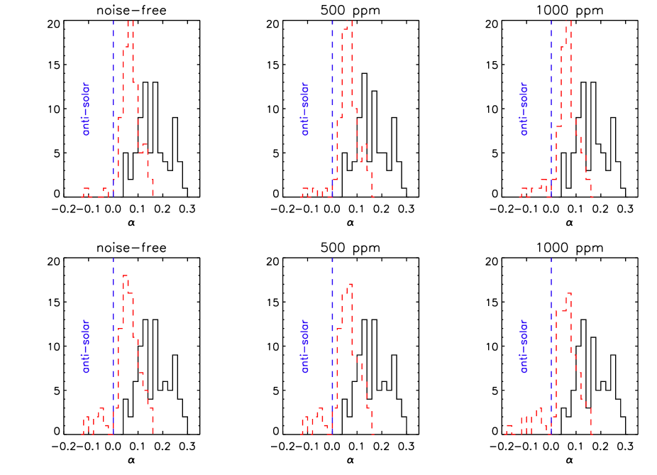
Figure 4: Distributions of $\alpha_{\rm model}$ (solid black) and $\alpha_{\rm obs}$ (dashed red) of the 10-spot model for different noise levels. Upper panel: No spot evolution, Lower panel: Spot evolution included. False-positive detections exhibiting $\alpha_{\rm obs}<0$ are located left of the dashed blue line (indicating $\alpha_{\rm obs}=0$).

4.3 Kepler data

In this section we apply our method to a sample of 50 selected Kepler stars. As shown previously our method performs well for simulated data. We were curious to see whether it is possible to detect the sign of DR in real data in general, especially answering the question for how many stars antisolar DR is revealed by our method. Therefore, we selected a hand-picked sample of solar-like stars from the Kepler archive. Although solar-like DR is expected for these stars, the underlying differential rotation law is still unknown.

The selected stars should hold the following criteria: surface gravities $\log g>3.5$, color index $0.60<B-V<0.92$ (roughly corresponding to spectral type G0–G9 using the $g-r$ to $B-V$ color transform from Jester et al. (2005)), and Kepler magnitude $kepmag<13$, leaving roughly 5,700 stars. Since we are only interested in rotation, the above sample was further reduced by discarding eclipsing binaries and KOIs. Two stars in the sample were characterized as hybrid pulsators (Uytterhoeven et al., 2011), and one star as $\gamma$ Doradus pulsator (Tkachenko et al., 2013). These stars were also discarded.

To minimize the effect of possible instrumental flaws we only selected stars with strong intrinsic variability, expressed in terms of the variability range $R_{\rm var}>0.3\,\%$ (Basri et al., 2011). Additionally, the most significant period in the periodogram should hold $1<P_{1}<25$ days. These limits should guarantee a stable rotational modulation over many rotation cycles.

We only used Kepler Q1–Q14 data, which were consistently reduced with the PDC-MAP pipeline (version 2.1–3.0). Q15–Q17 data have not been considered, because these data were reduced with the msMAP pipeline, which applies a 20 day high-pass filter to certain quarters, thus affecting the signal of slower rotators. The light curves were stitched together in a simple way by dividing each quarter by its median and subtracting unity. The light curves were smoothed with a 30-day window to remove remaining long-term trends, likely caused by the instrument.

Furthermore, we visually inspected all light curves and their periodograms. We only selected stars with multiple periodogram peaks, at least one visible harmonic, and clearly visible rotational modulation in the light curve. The above criteria and the visual inspection left only 50 stars in total.

Our method described in Sect. 3 was applied using the same constraints as for the simulated data. We found that the separation of the two peaks $P_{1}$ and $P_{2}$ on the frequency grid has a strong influence on the determination of the correct sign of DR. Therefore, we define

$$\Delta f:=|1/P_{1}-1/P_{2}|$$ (5)

To have a dimensionless quantity for the peak separation, we divide this frequency difference by the minimum frequency $f_{\rm min}=1/\max(\rm time)$ of the periodogram. In the following, the number of points on the frequency grid separating two peaks is called the peak separation. Forcing the program only to pick peaks with $\Delta f/f_{\rm min}\geq n$ with $n\geq 2$ rules out certain peak combinations. This happens, e.g., when more than two distinct rotation peaks are found, but only the two closest peaks exhibit a detectable harmonic. For this reason the total number of detections drops when increasing the minimum peak separation (s. second column in Table 2).

Table 2 summarizes the results and Fig. 5 shows the distribution of $\alpha_{\rm obs}$ using the different constraints. Increasing the minimum peak separation significantly reduces the total number of detections, especially the cases where the highest peaks have been chosen ($k_{\rm min}=1$). The number of detections of antisolar-type differential rotation varies from 28–37 %.

To put the Kepler results into context we applied our method to the 10-spot models including spot evolution and 1000 ppm white noise using the same peak separations as above. We found that reducing the minimum peak separation from five to two frequency bins increases the percentage of false-positives from 11.3 % to 20 %. The number of cases with $k_{\rm min}=1$ fluctuates between 78–91 %. This might suggest that the result for $\Delta f/f_{\rm min}\geq 2$ is least reliable, although $k_{\rm min}=1$ was used in all cases. Such split peaks with small peak separation are likely caused by spot evolution.

Peak sep.	# detections	# detections	Solar	Antisolar
$\Delta f/f_{\rm min}$	(total)	($k_{\rm min}=1$)	$\alpha>0$	$\alpha<0$
$\geq 2$	39	39	28	11
$\geq 3$	35	28	22	13
$\geq 4$	33	20	22	11
$\geq 5$	28	13	18	10

Table 2: Number of solar and antisolar detections out of the 50 Kepler stars. $\Delta f/f_{\rm min}$ denotes the minimum peak separation. The second column shows the total number of detections. Thereof, the number of detections with $k_{\rm min}=1$ is given in the third column. The last two columns denote the number of solar and antisolar detections, respectively.

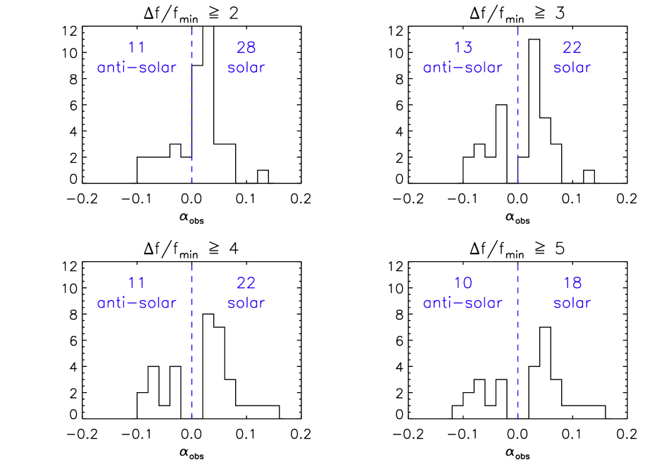
Figure 5: Distribution of $\alpha_{\rm obs}$ of the 50 Kepler stars forcing different minimum peak separations. The dashed blue line indicates rigid rotation ($\alpha_{\rm meas}=0$).

5 Discussion

As shown in the previous section, our method performs well for simulated data, especially the results of the 2-spot models are striking. The detection rate for the 10-spot models is still high, although the periodograms exhibit more than only two significant rotation peaks, as do their harmonics (see Fig. 2).

The false-positive rate of our method depends on the noise level, the minimum peak separation, and the presence of spot evolution. We found that our method is very robust against adding pure white noise to the light curves, in agreement with other studies (Reinhold & Reiners, 2013). Adding higher white noise to the light curves decreases the total number of detections, but does not significantly increase the false-positive rate. Spot evolution was found to be the major contributor of spurious detections. The largest rate was found for the 10-spot models including spot evolution and having small peak separations, increasing up to 20 % for the highest noise levels. In certain cases very short-lived spots can produce split rotation peaks, and thus mimic differential rotation.

In real data this effect becomes more important, because spot lifetimes are difficult to assess. In some situations spot evolution can barely be distinguished from DR, making the determination of the sign of DR is even harder. In general, periodograms of Kepler stars exhibit many more peaks, with some of them being spurious detections. Furthermore, the periodogram strongly depends on the length of time series. Since the peak width is proportional to the inverse of the total observing time span, a certain length of high-quality photometry is required to resolve individual peaks. But also the analysis of two different light curve segments of equal length may change the result. Spot evolution and differential rotation may be more “visible” in one segment than in the other, as revealed by their periodograms, either showing a single or multiple clear peaks, respectively. This effect immediately connects to the different peak separations (see Fig. 5). Computing the periodogram of the full time series averages out these effects. Therefore, analyzing different light curve segments might increase the sample of suitable candidates to test this method.

Unfortunately, the false-positive rate of our method cannot be transferred directly to Kepler data, because the percentage of real antisolar rotators is unknown. It should rather be interpreted as the number of cases where true solar rotators are misclassified as antisolar rotators, and vice versa. Since the light curves and periodograms of solar and antisolar rotators exhibit similar shapes, one can argue that both cases should be treated equally by the method, i.e., the rate of stars with wrongly determined sign of DR should be the same on either side. The measured number of antisolar detections then consists of the fraction of real antisolar rotators, which are actually detected as such, plus the number of migrated solar-like stars, misclassified as antisolar rotators. Thus, we define

$$\hskip 56.9055ptS^{\prime} = (1-f)S+fA$$ (6)

$$\hskip 56.9055ptA^{\prime} = (1-f)A+fS.$$ (7)

$S^{\prime}$ and $A^{\prime}$ are the measured solar and antisolar detections, respectively, $S$ and $A$ the number of real solar and antisolar rotators, respectively, and $f=0.2$ the maximum false-positive rate. Solving this system of linear equations yields

$$\hskip 56.9055ptA = \frac{(1-f)A^{\prime}-fS^{\prime}}{1-2f}$$ (8)

$$\hskip 56.9055ptS = A^{\prime}+S^{\prime}-A.$$ (9)

Applying this solution to the numbers given in Table 2 we detect solar DR in 21–34 and antisolar DR in 5–10 stars of our sample of 50 stars. Table 3 lists the KIC numbers of our sample of 50 Kepler stars, providing their differential rotation law found by our method for the different peak separations. Most of the stars are consistently found as solar (s) or antisolar (a) rotators, whereas some switch from one to the other. Additionally, one can see that forcing a larger peak separation leads to a non-detection (-) for some stars.

KIC	$\Delta f/f_{\rm min}\geq$
	2	3	4	5
1724975	s	s	s	s
3352189	a	a	-	-
3837480	s	s	s	-
3862793	-	-	-	-
4557559	s	s	s	a
4639291	a	a	a	a
4677300	s	s	s	s
4758719	a	a	a	a
4829624	-	-	-	-
5032950	s	s	s	s
5091941	s	s	s	s
5165799	s	s	s	s
5621105	s	s	s	s
6038355	a	a	a	a
6064684	s	s	s	s
6145471	s	s	s	-
6182131	a	a	a	a
6633742	-	-	-	-
6976397	s	a	a	-
7201168	s	s	s	s
7385442	a	a	a	a
7434544	s	s	s	s
7601913	a	-	-	-
7678060	s	-	-	-
7739728	s	-	-	-
7950229	-	-	-	-
8160546	s	s	s	s
8180580	-	-	-	-
8226464	a	a	a	a
8299279	s	s	s	s
8311074	s	a	a	a
8457754	s	s	s	a
8883245	-	-	-	-
8903403	s	a	a	a
8957218	s	s	s	s
9002888	s	s	s	s
9161418	-	-	-	-
9172729	s	s	s	s
9222547	-	-	-	-
9272360	-	-	-	-
9389733	a	a	a	-
9693116	-	-	-	-
9715600	s	s	s	s
10544691	s	s	s	s
10797565	a	a	a	-
11619829	a	a	s	s
11909695	-	-	-	-
12217823	s	s	-	-
12554089	s	-	-	-
12691333	s	s	s	s

Table 3: Solar (s) and antisolar (a) detections for the selected 50 Kepler stars depending on the peak separation.

As discussed above this new method performs well in our simulations, but should be used with caution in real data. Although we tried to successively approach the shape of real light curves by increasing the number of spots, probing the effect of spot evolution, and considering different noise scenarios, some effects have not been considered. The spot evolution as implemented in our model may be over-estimating real spot lifetimes. Furthermore, instrumental artifacts in the quarterly delivered Kepler data, and their reduction by the PDC-MAP pipeline certainly affect the overall light curve shape, and thus the period determination.

This number of antisolar detections seems quite large, but reflects the outcome of the method. Since the light curves created from the 10-spot models look very similar to real Kepler data, we are optimistic that our findings of antisolar DR are real, although independent measurements to either prove or disprove our results are urgently needed.