Anderson localization of Bogoliubov excitations on quasi-1D strips

Abstract

Anderson localization of Bogoliubov excitations is studied for disordered lattice Bose gases in planar quasi–one-dimensional geometries. The inverse localization length is computed as function of energy by a numerical transfer-matrix scheme, for strips of different widths. These results are described accurately by analytical formulas based on a weak-disorder expansion of backscattering mean free paths.

I Setting, Objectives, and Scope

Single-particle Anderson localization in quasi-1D geometries with correlated disorder is already a challenging problem Beenakker (1997); Tessieri and Izrailev (2006); Izrailev et al. (2012); Herrera-González et al. (2014). With interactions, the situation becomes even more interesting. Here, we study the localization properties of the Bogoliubov quasi-particles (BQP) of weakly disordered Bose gases at zero temperature on quasi-1D lattices. While interactions tend to screen the disorder and thus stabilize extended (quasi-)condensates Petrov et al. (2000) for weak disorder Lee and Gunn (1990); Müller and Gaul (2012), BQPs are expected to be localized irrespective of their energy or disorder strength in low dimensions John et al. (1983); Gurarie and Chalker (2003); Lugan et al. (2007), thus emulating noninteracting particles in the orthogonal Wigner-Dyson universality class Evers and Mirlin (2008). Yet, BQPs differ qualitatively from noninteracting particles because of their collective, phonon-like behavior at low energy. Moreover, they experience a randomness mediated by the inhomogeneous condensate background, which responds nonlinearly and nonlocally to the bare disorder Sanchez-Palencia (2006); Gaul and Müller (2011); Lugan and Sanchez-Palencia (2011). This interplay has been extensively examined in 1D Gurarie et al. (2008); Fontanesi et al. (2010); Lellouch and Sanchez-Palencia (2014); Vermersch et al. (2014), where direct backscattering provides the only pathway to localization.

In this Letter, we discuss the localization length of BQPs on quasi-1D planar lattices of transverse width $N\times 1$ (shown in Fig. 1a). While the techniques developed below also apply to $N_{x}\times N_{y}$ bars, strips provide the simplest realization of a multi-channel geometry, where phase-coherent scattering between modes is the rule. The bosons are described by the Bose-Hubbard (BH) model with on-site interaction $U>0$, hopping $t$ (with periodic boundary conditions across the strip) and on-site disorder $V_{\bm{x}}$. The random potential $V_{\bm{x}}$ is drawn from a Gaussian distribution and has no spatial correlation on the lattice scale, $\overline{V_{\bm{x}}V_{{\bm{x}}^{\prime}}}=\delta_{{\bm{x}}{\bm{x}}^{\prime}}V^{2}$, where the bar denotes disorder averaging and $V^{2}$ is the on-site variance. For each realization of disorder, the mean-field (MF) ground-state density $n_{\bm{x}}$ is determined by the condensate amplitude $\Phi_{\bm{x}}=\sqrt{n_{\bm{x}}}$ that solves the discrete Gross-Pitaevskii (GP) equation

$$-t\sum_{\langle{\bm{x}}{\bm{x}^{\prime}}\rangle}\Phi_{{\bm{x}^{\prime}}}+(2t+V_{{\bm{x}}})\Phi_{{\bm{x}}}+U\Phi_{{\bm{x}}}^{3} =\mu\Phi_{{\bm{x}}},$$ (1)

where the sum runs over the nearest neighbors of ${\bm{x}}$. The chemical potential $\mu$ controls the average occupation $n=\overline{n_{\bm{x}}}$. In the limit of large occupations Mora and Castin (2003), an expansion of the BH Hamiltonian around the MF solution yields the Bogoliubov-de Gennes (BdG) equations

$$-t\sum_{\langle{\bm{x}}{\bm{x}^{\prime}}\rangle}u_{{\bm{x}^{\prime}}}+[2t+V_{{\bm{x}}}+2Un_{{\bm{x}}}-\mu]u_{{\bm{x}}}+Un_{{\bm{x}}}v_{{\bm{x}}} =Eu_{{\bm{x}}}$$

$$-t\sum_{\langle{\bm{x}}{\bm{x}^{\prime}}\rangle}v_{{\bm{x}^{\prime}}}+[2t+V_{{\bm{x}}}+2Un_{{\bm{x}}}-\mu]v_{{\bm{x}}}+Un_{{\bm{x}}}u_{{\bm{x}}} =-Ev_{{\bm{x}}},$$ (2)

where $u_{{\bm{x}}}$ and $v_{{\bm{x}}}$ are the BQP particle and hole components at energy $E$. These Bogoliubov excitations determine ground-state properties as well as the (thermo-)​ ​ dynamical response of the system.

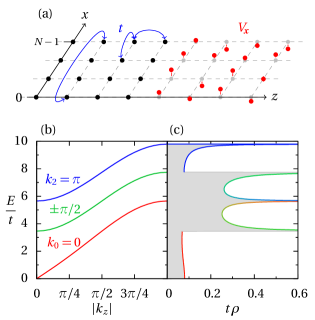
Figure 1: System configuration for the $4\times 1$ geometry. (a) Sketch of the discrete strip geometry, with hopping amplitudes indicated on the left and on-site disorder on the right. (b) Clean lattice Bogoliubov dispersion showing contributions from the transverse modes $k_{j}$, $(j=0,\dots,3)$. (c) Clean excitation DOS [cf. Eq. (3)] with 1D divergencies at channel openings. The color code indicates the relative contribution of the individual transverse modes. All distances are given in units of lattice spacing. Panels (b) and (c) are drawn for $Un/t=2.0$.

In the remainder of this paper, we compute the dependence of the BQP localization length on the excitation energy. We first present a numerical transfer-matrix method that provides us with precise estimates of the localization length over a wide range of parameters (section II). Then we develop an analytical framework that combines random-matrix theory Beenakker (1997) with a microscopic transport theory (section III). In particular, we find that the predictions using a lattice Boltzmann mean-free path are in excellent agreement with the numerics.

II Numerical transfer-matrix calculations

Our numerical calculations of the localization length follow a standard transfer-matrix scheme Pichard and Sarma (1981); Kramer and MacKinnon (1993); Beenakker (1997); Slevin and Ohtsuki (2014): The BdG equations (I) are cast into the recursive form ${\bm{w}}_{i+1}=M_{i}{\bm{w}}_{i}$, where the $4N$-component vector ${\bm{w}}_{i}$ encodes the values of $u_{\bm{x}}$ and $v_{\bm{x}}$ on two neighboring lattice slices at $z=i$ and $z=i-1$ (throughout the article, distances are expressed in units of lattice spacing). The transfer matrix $M_{i}$ is parametrized by $E$ as well as the values of $V_{\bm{x}}$ and $n_{{\bm{x}}}$ on slice $i$. The propagation of the BdG excitations along $z$, from an arbitrary initial condition ${\bm{w}}_{0}$, then simply amounts to matrix-vector multiplication. Via this procedure, the estimator $\ln\|{\bm{w}}_{L}\|/L$ yields, with probability one, the largest Lyapunov exponent $\lambda_{1}$ in the limit $L\to\infty$. The $r$ largest Lyapunov exponents $\lambda_{1}>\dots>\lambda_{r}$ are retrieved similarly, by propagating a frame of $r$ linearly independent initial vectors ${\bm{w}}_{0}^{[j]}$ ($j=1,\dots,r$), enforcing their orthogonality during propagation, and monitoring their exponential growth (to maintain numerical accuracy, we performed a Gram-Schmidt orthonormalization every 8 sites). As the BQP Lyapunov exponents come in pairs of opposite sign, $2N$ vectors are required to calculate the smallest positive Lyapunov exponent $\lambda=\lambda_{2N}$, identified as the inverse localization length $1/l_{\rm loc}$ Beenakker (1997); Slevin and Ohtsuki (2014).

One crucial advantage of the transfer-matrix approach is the self-averaging of the $\ln\|{\bm{w}}_{L}^{[j]}\|/L$ estimators, whose relative fluctuations decrease as $1/\sqrt{L}$. The propagation of one set of initial vectors over a large distance $L$ thus suffices to compute the Lyapunov spectrum with the desired precision. Such a scheme is easy to implement with an uncorrelated random potential, as the purely local random values of $V_{\bm{x}}$ can be generated on the fly. In the case of BQPs, however, the GP equation (1) implies a global minimization problem that is already intractable for the size required to achieve only 10% accuracy on the Lyapunov exponents. In our calculations, we chained quasi-1D segments of length $L_{0}=2^{14}$ and, on each segment, solved Eq. (1) at fixed density $n$ with a conjugate-gradient technique Modugno et al. (2003); Saliba et al. (2014). While each segment interface introduces a slight mismatch in $\mu$, and also in $n_{\bm{x}}$ over typically $\sqrt{t/(Un)}$ sites, the impact of these artifacts on $\lambda$ vanishes with increasing $L_{0}$. We checked that all the results presented here are converged with respect to the choice of $L_{0}$. To ensure a sufficient scrambling of initial data and speed up estimations, we chained up to 64 segments and averaged the $\ln\|{\bm{w}}_{L}^{[j]}\|$ data over 200 independent propagations.

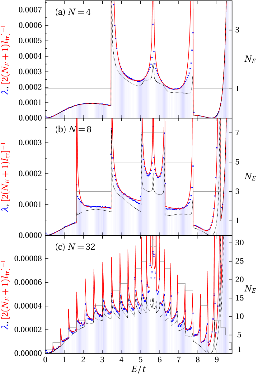
Figure 2: Inverse localization length $\lambda$ (error bars indicate the error of the mean after averaging over 500 configurations in (a) and (b) and 225 in (c), and are hardly appreciable on the scale of the plot) and its estimates from transport theory as a function of energy. The dashed line is $[(N_{E}+1)l_{\text{bs}}]^{-1}$ from Eq. (5), and the solid red line is $[2(N_{E}+1)l_{\text{tr}}]^{-1}$ from Eq. (6). The staircase-like line indicates the number of open channels $N_{E}$ (scale on the right border). Parameters: hopping $Un=2t\approx\mu$, i.e., the transition from sound waves to particle excitations is around $E/t=2$. Disorder strength $V=0.1Un$.

Figure 2 shows the inverse localization length $\lambda$ as function of energy for various strip widths $N$. For all $N$ we observe two important features. First, $\lambda$ diverges at the inner band edges, where the channels of the clean system open or close (cf. Fig. 1c) and thus contribute a divergent 1D density of states (DOS), which results in strong scattering and thus localization on short length scales. Second, for an equal number of open channels and once inner divergences are disregarded, $\lambda$ displays a similar trend as in 1D Lugan et al. (2007), increasing with $E$ in the phonon regime $E\lesssim Un$, and decreasing in the free-particle regime $E\gtrsim Un$.

III Analytical transport theory

For quasi-1D strips, random-matrix theory Beenakker (1997) predicts that the localization length $l_{\rm loc}=2(N_{E}+1)l_{\text{tr}}$ is proportional to the transport mean free path $l_{\text{tr}}$. Here, $N_{E}$ is the number of open channels at energy $E$. In this section, we validate this prediction using two different analytical expressions for the mean free path.

The clean system is discrete translation invariant, and therefore the free-particle dispersion relation is diagonal in momentum, $\epsilon^{0}_{{\bm{k}}}=2t\sum_{i=x,z}[1-\cos(k_{i})]$. The dispersion of Bogoliubov excitations then reads as usual $\epsilon_{{\bm{k}}}=[\epsilon^{0}_{{\bm{k}}}(\epsilon^{0}_{{\bm{k}}}+2Un)]^{1/2}$. On the strip, the momentum ${\bm{k}}=(k_{j},k_{z})$ is transverse quantized as $k_{j}=2\pi j/N$ under periodic boundary conditions with $j=0,\dots,N-1$, thus defining the $N$ possible channels. In terms of the longitudinal group velocity $v_{\bm{k}}=\partial\epsilon_{{\bm{k}}}/\partial k_{z}$ (all velocities here and below refer to the $z$-component), the DOS per unit length and transverse size is expressed as

$$\rho(E)=\frac{1}{N}\sum_{j=0}^{N-1}\int_{-\pi}^{\pi}\frac{dk_{z}}{2\pi}\delta(E-\epsilon_{{\bm{k}}})=\frac{1}{2\pi N}\sum_{{\bm{k}}\in S_{E}}|v_{\bm{k}}|^{-1}.$$ (3)

$S_{E}$ denotes the energy shell in momentum space, namely the set of points ${\bm{k}}$ such that $\epsilon_{{\bm{k}}}=E$. Its cardinality $|S_{E}|=2N_{E}$ counts both forward and backward propagating channels with $k_{z}>0$ and $k_{z}<0$, respectively. The clean DOS is plotted in Fig. 1c. The opening and closing of each channel produces a characteristic van Hove divergence. Near the divergence, essentially only one channel matters. In between these singularities several channels mix, as indicated by the color coding in the plot.

The disorder potential produces elastic scattering out of a given mode ${\bm{k}}$ with a rate $\gamma_{\bm{k}}=2\pi\sum_{\bm{p}}\delta(\epsilon_{\bm{k}}-\epsilon_{{\bm{p}}})\overline{|W_{{\bm{k}}{\bm{p}}}|^{2}}$. Here $W_{{\bm{k}}{\bm{p}}}=V_{{\bm{k}}-{\bm{p}}}w_{{\bm{k}}{\bm{p}}}$ is a (first-order) matrix element of the disordered Bogoliubov Hamiltonian, namely the bare disorder Fourier component $V_{{\bm{k}}-{\bm{p}}}$ dressed by an envelope

$$w_{{\bm{k}}{\bm{p}}}{=}\frac{(\epsilon^{0}_{\bm{k}}+Un)\epsilon^{0}_{{\bm{k}}-{\bm{p}}}-2Un\epsilon^{0}_{\bm{k}}}{\epsilon_{\bm{k}}(2Un+\epsilon^{0}_{{\bm{k}}-{\bm{p}}})}\qquad(\epsilon^{0}_{{\bm{k}}}=\epsilon^{0}_{{\bm{p}}})$$ (4)

that accounts for the underlying nonlinearities Gaul and Müller (2011, 2013). [Eq. (4) is the on-shell value $w_{{\bm{k}}{\bm{p}}}^{(1)}|_{\epsilon^{0}_{{\bm{k}}}=\epsilon^{0}_{{\bm{p}}}}$ given by Eqs. (13) – (15) in Gaul and Müller (2013) or, equivalently, the lattice version of Eq. (14) in Gaul and Müller (2008).] The associated elastic mean free path is then the group velocity divided by the scattering rate. Since localization along the $z$ direction can only be caused by scattering events that flip the momentum $z$-component, we consider the backscattering mean free path

$$l_{\text{bs}}(E)^{-1}=\min_{{\bm{k}}\in S_{E}}\frac{V^{2}}{N|v_{\bm{k}}|}{\sum_{{\bm{p}}}}^{\prime}|v_{\bm{p}}|^{-1}w_{{\bm{k}}{\bm{p}}}^{2}\ .$$ (5)

The primed sum runs only over those momenta ${\bm{p}}\in S_{\epsilon_{{\bm{k}}}}$ with $z$-components of opposite sign, $\mathrm{sgn}(p_{z}k_{z})=-1$. Moreover, we take the shortest inverse mean free path at a given energy $E$ since the numerics produce the smallest localization exponent. The resulting prediction $[(N_{E}+1)l_{\text{bs}}(E)]^{-1}$ is plotted as the dashed line in Fig. 2. There is already some overall qualitative agreement, which becomes even quantitative at low and high energies, where only a single channel contributes. And indeed, in this case ($N_{E}=1$) one has $2\pi N\rho(E)=2|v_{k}|^{-1}$ at $\epsilon_{k}=E$, and thus the estimate for the Lyapunov exponent $(2l_{\text{bs}})^{-1}=V^{2}w_{k(-k)}^{2}/(2Nv_{k}^{2})$ agrees with the established theoretical result Lugan et al. (2007); Lugan and Sanchez-Palencia (2011); Gaul and Müller (2011).

The number $N_{E}$ of open channels is also plotted in each figure. With more open channels, the estimate involving $l_{\text{bs}}$ becomes less reliable, which becomes especially obvious near the center of plots b) and c) for the $8\times 1$ and $32\times 1$ geometries. The agreement deteriorates even further if only diagonal backscattering into the same channel ($p_{j}=k_{j}$ and $p_{z}=-k_{z}$) is taken into account.

We therefore try to improve on our estimate and consider the lattice version of the full Boltzmann transport mean free path, which can be derived within linear-response quantum transport theory Kuhn et al. (2007); Kuhn (2007). With the notations introduced above, this gives

$$l_{\text{tr}}(E)^{-1} =\frac{V^{2}}{2\pi N^{2}\rho(E)\langle v^{2}\rangle_{E}^{3/2}}\sum_{{{\bm{k}},{\bm{p}}\in S_{E}}}\!\frac{v_{\bm{p}}(v_{\bm{p}}-v_{\bm{k}})w_{{\bm{k}}{\bm{p}}}^{2}}{|v_{\bm{p}}||v_{\bm{k}}|}$$ (6)

Here, $\langle v^{2}\rangle_{E}=\sum_{{\bm{k}}\in S_{E}}|v_{\bm{k}}|/[{2\pi}N\rho(E)]$ denotes an energy-shell average. The usual factor $(1-\cos\theta)$ in scattering angle $\theta$ under the momentum integral (see, e.g., (Gaul and Müller, 2011, Fig. 6) and (Kuhn et al., 2005, Eq. (6))) is now represented by $(v_{\bm{p}}-v_{\bm{k}})$. The factors of $|v_{\bm{k}}|$ and $|v_{\bm{p}}|$ in the denominator stem from the $k_{z}$-integrals over on-shell spectral functions, analogous to the second equality in (3).

For a strict 1D problem, i.e., for a single open channel ($N_{E}=1$), this expression reduces to $2l_{\text{tr}}=l_{\text{bs}}$, as it should (Beenakker, 1997, Eq. (152)). But also when several channels are open, the agreement with the numerical data is clearly excellent, as shown in Fig. 2. Remarkably, Eq. (6) performs especially well in between the 1D resonances, where the coherent coupling between channels has to be described rather accurately.

Of course, the result (6) is perturbative in nature, essentially valid for weak enough disorder ($V\ll Un$), and thus only holds if the (quasi-)condensate is extended. For much stronger disorder, the condensate fragments and the Bose fluid enters the non-superfluid, Bose-glass phase Fontanesi et al. (2011); Saliba et al. (2014).

IV Summary and Outlook

In conclusion, we have calculated the localization length for Bogoliubov excitations of Bose-Einstein condensates on disordered lattices with a planar quasi-1D geometry. Numerical data from a transfer-matrix computation are very well reproduced by an analytical formula adapted from continuum transport theory. Our approach could extend to larger systems $N\times 1$ (and $N\times N$) with $N\to\infty$ using finite-size scaling and thus yield the full 2D (and 3D) localization lengths, with the aim to track down possible mobility edges for BQPs in dimensions higher than 1.

References

- Beenakker (1997) C. W. J. Beenakker, Rev. Mod. Phys. 69, 731 (1997).
- Tessieri and Izrailev (2006) L. Tessieri and F. M. Izrailev, J. Phys. A: Math. Gen. 39, 11717 (2006).
- Izrailev et al. (2012) F. Izrailev, A. Krokhin, and N. Makarov, Phys. Rep. 512, 125 (2012).
- Herrera-González et al. (2014) I. F. Herrera-González, J. A. Méndez-Bermúdez, and F. M. Izrailev, Phys. Rev. E 90, 042115 (2014).
- Petrov et al. (2000) D. S. Petrov, G. V. Shlyapnikov, and J. T. M. Walraven, Phys. Rev. Lett. 85, 3745 (2000).
- Lee and Gunn (1990) D. K. K. Lee and J. M. F. Gunn, J. Phys.: Condens. Matter 2, 7753 (1990).
- Müller and Gaul (2012) C. A. Müller and C. Gaul, New J. Phys. 14, 075025 (2012).
- John et al. (1983) S. John, H. Sompolinsky, and M. J. Stephen, Phys. Rev. B 27, 5592 (1983).
- Gurarie and Chalker (2003) V. Gurarie and J. T. Chalker, Phys. Rev. B 68, 134207 (2003).
- Lugan et al. (2007) P. Lugan, D. Clément, P. Bouyer, A. Aspect, and L. Sanchez-Palencia, Phys. Rev. Lett. 99, 180402 (2007).
- Evers and Mirlin (2008) F. Evers and A. D. Mirlin, Rev. Mod. Phys. 80, 1355 (2008).
- Sanchez-Palencia (2006) L. Sanchez-Palencia, Phys. Rev. A 74, 053625 (2006).
- Gaul and Müller (2011) C. Gaul and C. A. Müller, Phys. Rev. A 83, 063629 (2011).
- Lugan and Sanchez-Palencia (2011) P. Lugan and L. Sanchez-Palencia, Phys. Rev. A 84, 013612 (2011).
- Gurarie et al. (2008) V. Gurarie, G. Refael, and J. T. Chalker, Phys. Rev. Lett. 101, 170407 (2008).
- Fontanesi et al. (2010) L. Fontanesi, M. Wouters, and V. Savona, Phys. Rev. A 81, 053603 (2010).
- Lellouch and Sanchez-Palencia (2014) S. Lellouch and L. Sanchez-Palencia, Phys. Rev. A 90, 061602 (2014).
- Vermersch et al. (2014) B. Vermersch, D. Delande, and J. C. Garreau, arXiv:1410.2587 (2014).
- Mora and Castin (2003) C. Mora and Y. Castin, Phys. Rev. A 67, 053615 (2003).
- Pichard and Sarma (1981) J. L. Pichard and G. Sarma, J. Phys. C 14, L617 (1981).
- Kramer and MacKinnon (1993) B. Kramer and A. MacKinnon, Rep. Prog. Phys. 56, 1469 (1993).
- Slevin and Ohtsuki (2014) K. Slevin and T. Ohtsuki, New J. Phys. 16, 015012 (2014).
- Modugno et al. (2003) M. Modugno, L. Pricoupenko, and Y. Castin, Eur. Phys. J. D 22, 235 (2003).
- Saliba et al. (2014) J. Saliba, P. Lugan, and V. Savona, Phys. Rev. A 90, 031603 (2014).
- Gaul and Müller (2013) C. Gaul and C. A. Müller, Eur. Phys. J. ST 217, 69 (2013).
- Gaul and Müller (2008) C. Gaul and C. A. Müller, Europhys. Lett. 83, 10006 (2008).
- Kuhn et al. (2007) R. Kuhn, O. Sigwarth, C. Miniatura, D. Delande, and C. A. Müller, New J. Phys. 9, 161 (2007).
- Kuhn (2007) R. Kuhn, Coherent Transport of Matter Waves in Disordered Optical Potentials, Ph.D. thesis, Universität Bayreuth & Université de Nice Sophia–Antipolis (2007).
- Kuhn et al. (2005) R. C. Kuhn, C. Miniatura, D. Delande, O. Sigwarth, and C. A. Müller, Phys. Rev. Lett. 95, 250403 (2005).
- Fontanesi et al. (2011) L. Fontanesi, M. Wouters, and V. Savona, Phys. Rev. A 83, 033626 (2011).