Lagrangian transport through surfaces in volume-preserving flows

Abstract

Advective transport of scalar quantities through surfaces is of fundamental importance in many scientific applications. From the Eulerian perspective of the surface it can be quantified by the well-known integral of the flux density. The recent development of highly accurate semi-Lagrangian methods for solving scalar conservation laws and of Lagrangian approaches to coherent structures in turbulent (geophysical) fluid flows necessitate a new approach to transport from the (Lagrangian) material perspective. We present a Lagrangian framework for calculating transport of conserved quantities through a given surface in $n$-dimensional, fully aperiodic, volume-preserving flows. Our approach does not involve any dynamical assumptions on the surface or its boundary.

1 Introduction

The transfer of a quantity along the motion of some carrying fluid, or Lagrangian transport for short, is of fundamental importance to a broad variety of scientific fields and applications. The latter include (geophysical) fluid dynamics [30, 37, 34, 20], chemical kinetics [4], fluid engineering [31, 35] and plasma confinement [3]. Existing methods for computing transport (i) have mostly been developed under certain assumptions on temporal behavior (steady or periodic time-dependence) [23, 24, 22, 33]; spatial location (regions related to invariant manifolds such as lobe dynamics and dividing surfaces in transition state theory) [23, 24, 22, 33, 25, 1]; state space dimension (2D) [23, 33, 25, 1]; or (ii) restrict to a perturbation setting [1]. Recently, the problem of quantifying finite-time transport in aperiodic flows between distinct, arbitrary flow regions has been considered by Mosovsky et al. [28]. They present a framework for describing and computing finite-time transport in $n$-dimensional (chaotic) volume-preserving flows, which relies on the reduced dynamics of an ($n-2$)-dimensional ‘minimal set’ of fundamental trajectories. In this paper, we present a Lagrangian approach to the complementary problem of computing transport through a codimension-one surface over a finite-time interval in volume-preserving flows. This cannot be reformulated in the setting of [28], since (i) initial and final positions of surface-crossing particles are a priori unknown, and (ii) particles may cross the surface several times, possibly in opposite directions, leading to a net number of surface crossings different from one, in particular including zero.

The problem of computing the flux through a surface in general flows admits a well-known solution in terms of an integral of the flux density over the surface and the time interval of interest, cf. the left-hand side of Eq. (1). We view this approach as Eulerian, in that it involves instantaneous information (flux density) at fixed locations in spacetime. Recently, two lines of research emerged that inevitably require a Lagrangian approach to the flux calculation.

The first is concerned with the numerical solution of advection equations (or, in the absence of sources, conservation laws) for conserved quantities by semi-Lagrangian methods, which enjoy geometric flexibility and the absence of Eulerian stability constraints [38, 39]. Roughly speaking, the term semi-Lagrangian refers to methods which evolve material densities on spatially fixed test volumes based on short-term material advection steps.

The second is concerned with transport by coherent vortices in oceanic flows, more precisely with the determination of the relevance of coherent transport [6, 42, 17], an open problem in physical oceanography and climate science. Coherent structures have long been studied in fluid dynamics [7], typically from an Eulerian point of view, i.e., by defining coherent structures as subsets of spacetime, usually as (sub-)level sets of scalar fields on spacetime [26, 32, 6, 42]. This approach, however, yields coherent structures with a priori unclear relation to actual fluid motion and hence ambiguous role in coherent transport; see transfer-operator related approaches which seek Eulerian coherent sets with minimal flux through the boundary under advection with small-scale diffusion superimposed, cf., for instance, [9]. For these reasons, Lagrangian approaches to coherent structures have been developed over the last few years. These seek coherent structures as subsets of the material evolving under the flow [14, 15, 18, 13, 10, 11, 21, 29], building on a wide variety of mathematical principles. The location of a material structure in spacetime is fully determined by its motion.

This implicit spatial definition of material structures poses a severe challenge to determining their contribution to transport through a surface in an Eulerian manner. First, for each point on the extended surface in spacetime knowledge is required whether it is occupied by a particle originating from the material structure of interest. Second, the subset of points on the surface which are occupied by material particles of interest may be very complicated, cf. Fig. 1, especially in turbulent flows. As a consequence, an Eulerian integration of the flux density restricted to the intersection of the extended surface with the path of the material set of interest is practically infeasible.

 

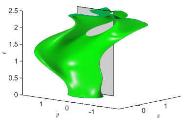
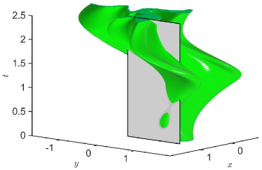
Figure 1: Views from opposite directions on the evolution of an initial ellipse over time, and its intersection with a surface in extended state space. Computing the flux contribution by the material points originating from that ellipse in an Eulerian framework corresponds to computing the flux integral over the subset of the section which is contained in the interior of the cylindrical structure.

Conversely, from the material point of view, it is intuitive that the number of surface crossings of each individual Lagrangian particle is relevant to determine its flux contribution. First steps towards a classification of Lagrangian particles with respect to net number of curve crossings have been proposed for two-dimensional flows under additional technical assumptions by Zhang [40, 41]. In this paper, we solve the following more general donating region problem [39, Def. 1.2].

Problem 1

For a given regular, divergence-free and time-dependent vector field $\boldsymbol{u}(t,\boldsymbol{x})=\boldsymbol{u}_{t}(x)$, consider a conserved quantity $f(t,x)=f_{t}(x)$, which satisfies the scalar conservation law in Eulerian form

$$\partial_{t}f+\boldsymbol{u}_{t}\boldsymbol{\cdot\nabla}f=0.$$

Let $\mathcal{C}$ be a compact, connected, embedded codimension-one surface in (configuration space) $\mathbb{R}^{n}$, and $\mathcal{T}=[0,\tau]$ be a compact time interval. The problem is to find pairwise disjoint sets $\mathcal{D}_{k}\subset\mathbb{R}^{n}$, indexed by $k\in\mathbb{Z}$, of Lagrangian particles at time $t=0$, such that

$$\int_{\mathcal{C}\times\mathcal{T}}f_{t}(x)\cdot\boldsymbol{u}_{t}(x)\boldsymbol{\cdot}\boldsymbol{n}(x)\,\mathrm{d}x\,\mathrm{d}t=\sum_{k\in\mathbb{Z}}\thinspace k\cdot\int_{\mathcal{D}_{k}}f_{t}\bigr{|}_{t=0}(p)\,\mathrm{d}p,$$ (1)

where $\boldsymbol{n}$ is the unit normal vector field to $\mathcal{C}$ characterizing the direction of positive flux.

In fact, we may generalize Problem 1 and drop the assumption that $\mathcal{C}$ be stationary over $\mathcal{T}$. Thus, we solve the analogous problem for smoothly moving surfaces $\mathcal{H}=\bigcup_{t\in\mathcal{T}}\mathcal{C}_{t}$, i.e., $\mathcal{H}$ is everywhere transversal to time fibers $\{t\}\times\mathbb{R}^{n}$.

Problem 2

Let $\boldsymbol{u}(t,\boldsymbol{x})=\boldsymbol{u}_{t}(x)$ and $f(t,x)=f_{t}(x)$ be as in Problem 1, and $\hat{\boldsymbol{u}}_{t}(x)=\left(\begin{smallmatrix}1\\ \boldsymbol{u}_{t}(x)\end{smallmatrix}\right)$ the extended velocity field. Let $\mathcal{H}$ be a codimension-one surface in extended configuration space $\mathcal{T}\times\mathbb{R}^{n}$, $\mathcal{T}=[0,\tau]$, as defined above. The problem is to find pairwise disjoint sets $\mathcal{D}_{k}\subset\mathbb{R}^{n}$, indexed by $k\in\mathbb{Z}$, of Lagrangian particles at time $t=0$, such that

$$\int_{\mathcal{H}}f_{t}(x)\cdot\hat{\boldsymbol{u}}_{t}(x)\boldsymbol{\cdot}\hat{\boldsymbol{n}}_{t}(x)\,\mathrm{d}(t,x)=\sum_{k\in\mathbb{Z}}\thinspace k\cdot\int_{\mathcal{D}_{k}}f_{t}\bigr{|}_{t=0}(p)\,\mathrm{d}p,$$ (2)

where $\hat{\boldsymbol{n}}_{t}(x)$ is the unit normal vector field to $\mathcal{H}$ at $(t,x)$.

For ease of presentation, we will first focus on the stationary case as in Problem 1, before we discuss the general case as in Problem 2 in Section 5.

2 Illustrative discussion of the main result

The aim of this section is to discuss Eq. (1) in anticipation of mathematical constructions presented in Sections Section 3 and Section 4. In fact, those constructions emerge naturally when taking a differential topological view on the change from Eulerian to Lagrangian coordinates. We recall and discuss concepts related to that coordinate change in Section 3.

First, the left-hand side of Eq. (1) corresponds to the classical flux integral over the surface $\mathcal{C}$ over time $\mathcal{T}$. The integrand, also called the flux density, corresponds to the normal component of the velocity field weighted with the material density $f$. Here, the flux is viewed from the perspective of the section, which is why we refer to the left-hand side of Eq. (1) as the Eulerian flux integral.

In contrast, the right-hand side of Eq. (1) is an integral, or a sum of integrals, solely over material points or particles. As our later analysis reveals we may decompose the whole material domain (up to a measure zero set) into disjoint material subsets, each of which contains particles with a certain number of net crossings across the surface $\mathcal{C}$ over the time interval $\mathcal{T}$. These material subsets are denoted by $\mathcal{D}_{k}$, where $k$ refers to the net number of transversal crossings, and have been coined donating regions of fluxing index $k$ by Zhang [41]. The contribution to transport by each donating region corresponds to its respective mass (or volume in a homogeneous fluid) multiplied by its corresponding fluxing index. The overall transport through $\mathcal{C}$ is then given by the sum of transport contributions of all donating regions. In summary, the right-hand side of Eq. (1) views the flux from the perspective of the mass-carrying particles, which is why we refer to it as the Lagrangian flux integral.

For illustration, consider an array of vortices, given by the stream function

$$H(x,y)=-A\sin\left(\pi x\right)\sin\left(\pi y\right),$$

subject to an aperiodic, spatially uniform spiraling forcing given by

$$F(t)=\left(t\sin\left(\pi t\right),t\cos\left(\pi t\right)\right)^{\top}.$$

The velocity field is hence

$$\boldsymbol{u}(t,x,y)=\begin{pmatrix}\phantom{-}\partial_{y}H(x,y)-t\sin\left(\pi t\right)\\ -\partial_{x}H(x,y)-t\cos\left(\pi t\right)\end{pmatrix}.$$

We set the section to $\mathcal{C}=\left\{x=0.75,\thinspace-0.2\geq y\geq 1.2\right\}$, the time interval to $\mathcal{T}=\left[0,2.5\right]$, and, for simplicity, the material density $f\equiv 1$. Fig. 2 shows the regions of particles with fluxing index $+1$, $0$, and $-1$; here, white corresponds to fluxing index $0$. For details on how to construct the donating regions, see Section 4.4. There are no particles with other fluxing indices, and some particles attain a fluxing index $+1$ by crossing twice in positive and once in negative direction, such as the sample trajectory shown in red.

For a numerical validation of Eq. (1), we compute its left-hand side by numerical quadrature, which yields a transport value of $-0.142$. For the right-hand side, we subtract the area of $\mathcal{D}_{-1}$ from that of $\mathcal{D}_{1}$, and obtain a transport value of $-0.141$, with relative error below $1\%$. For further improvements of area calculations via spline-approximation of polygon boundaries see [38]. Note that, in practice, the numerical integration of the Eulerian integral becomes more challenging in case the section $\mathcal{C}$ is curved and requires a parametrization. In contrast, we will see that a curved section does not add any difficulty in the Lagrangian framework. This geometric flexibility has been one major motivation to develop semi-Lagrangian numerical schemes for solving conservation laws, cf. [38, 41].

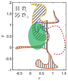
Figure 2: Donating regions divided in cells with fluxing index $+1$ (vertically hatched), $-1$ (diagonally hatched) and $0$ (white). The dashed curve (red) is a sample trajectory (path line). The ellipse (dark green) corresponds to the set of Lagrangian particles whose flow evolution is shown in Fig. 1.

For our main intended application, the calculation of the contribution to transport by a certain material subset $A$—such as the ellipse in Figs. 1 and 2 (dark green, centered at $(0.3,0.5)$ with semi-major axis $0.6$ in $y$-direction, and semi-minor axis $0.4$ in $x$-direction)—reduces to subtracting the area of $A\cap\mathcal{D}_{-1}$ from $A\cap\mathcal{D}_{1}$, which yields $-0.1061$.

At first sight, this may seem paradoxical, since the entire ellipse is launched from one side of the section. Fig. 1 now indicates that at the end of the time interval, parts of the material ended up on the other side of the section. Going from the first to the latter side corresponds to positive flux, and one would expect an overall positive transport contribution. However, a closer inspection of Fig. 1 reveals that most of the material which is advected to the other side has actually not crossed the section, but has flown around it. Moreover, much of the material which has flown around has actually crossed the section in negative direction, thus yielding an overall negative flux contribution of the ellipse.

The rest of this paper is devoted to the derivation of Eqs. (1) and (2). Most of the involved abstract concepts turn out to have a nice physical interpretation.

3 Eulerian and Lagrangian coordinates

While Eulerian coordinates $x$ are assigned to spatial points in a fixed frame of reference, Lagrangian coordinates $p$ label material points and are usually taken as the Eulerian coordinates at some initial time, say, $t=0$. The motion of material points is described by the flow $\varphi$, a mapping between initial positions $p$ at time $t=0$ and current positions $x$ at time $t$, i.e., $\varphi_{0}^{t}(p)=x$. Thus, the flow map $\varphi_{0}^{t}$ can be interpreted as a change from Lagrangian to Eulerian coordinates. The inverse flow map $\varphi_{t}^{0}=\left(\varphi_{0}^{t}\right)^{-1}$ corresponds then to the change from Eulerian to Lagrangian coordinates.

In fluid dynamics, there are two important characteristic curves associated with the flow [2], which we re-interpret in terms of Eulerian and Lagrangian coordinates.

A path line through $p$ is the time-curve of a fixed Lagrangian particle $p$ in Eulerian coordinates, i.e., $t\mapsto\varphi_{0}^{t}(p)$. In other words, the path line is a collection of Eulerian positions that the Lagrangian particle $p$ will occupy at some time. Its time derivative, expressed in Eulerian coordinates, gives rise to the velocity field

$$\boldsymbol{u}_{t}(x)\coloneqq\boldsymbol{u}(t,x)=\partial_{t}\varphi_{0}^{t}(\varphi_{t}^{0}(x)).$$ (3)

By construction, the path line through $p$ is the solution of the initial value problem

$$\dot{x} =\boldsymbol{u}_{t}(x), x(0) =p.$$

A streak line through $x$ is the time-curve of a fixed Eulerian location $x$ in Lagrangian coordinates, i.e., $t\mapsto\varphi_{t}^{0}(x)$. In other words, the streak line is a collection of material points that will occupy the Eulerian position $x$ at some time, see Fig. 3. Our definition of streak lines suits well the currently intended purpose and is consistent with Zhang’s use [41]. It is more common and actually more intuitive, however, to view a streak line as the collection of material points that have passed the Eulerian position $x$ at some time. In this context, a streak line can be imagined as an instantaneous curve of Lagrangian markers, injected in the past at $x$ and passively advected by the flow, see [2]. The time derivative of the streak line, expressed in Lagrangian coordinates, gives rise to the streak vector field

$$\boldsymbol{w}_{t}(p)\coloneqq\boldsymbol{w}(t,p)=\partial_{t}\varphi_{t}^{0}(\varphi_{0}^{t}(p)).$$

By construction, the streak line through $x$ is the solution of the initial value problem

$$\dot{p} =\boldsymbol{w}_{t}(p), p(0) =x.$$

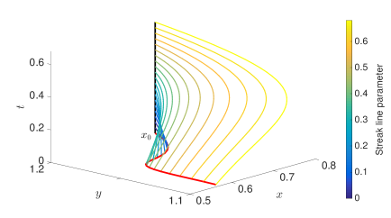
Figure 3: Streak line and streak vector field: the streak line through $x_{0}$ (red) is constructed by subsequently advecting $x_{0}$ from time $t$ backwards to time 0. Conversely, when a particle from the streak line, with curve parameter $s$ (colorbar), is launched at time 0 and advected $s$ time units, the particle reaches the spatial position $x_{0}$ (black). The streak vector field corresponds to the velocity of the streak lines. The bottom $x$-$y$-plane is to be considered as Lagrangian coordinates. Correspondingly, the streak vector field is a material vector field, in contrast to the classic velocity field, which is a spatial vector field.

To derive an algebraic relation between the velocity field $\boldsymbol{u}$ and the streak vector field $\boldsymbol{w}$, we compute the velocity $\partial_{t}\varphi_{t}^{0}(x)$ along the streak line $t\mapsto\varphi_{t}^{0}(x)$ through $x$. Differentiation of the constant function $t\mapsto\varphi_{0}^{t}\left(\varphi_{t}^{0}(x)\right)=x$ with the shorthand notation $p=\varphi_{t}^{0}(x)$ yields

$$0=\partial_{t}\varphi_{0}^{t}\left(p\right)+\mathrm{d}\varphi_{0}^{t}\left(p\right)\partial_{t}\varphi_{t}^{0}\left(x\right).$$

Using Eq. (3) and the invertibility of the linearized flow map with $\mathrm{d}\varphi_{0}^{t}\left(p\right)^{-1}=\mathrm{d}\varphi_{t}^{0}\left(x\right)$, we obtain

$$\begin{split}\boldsymbol{w}_{t}(p)=&-\left(\mathrm{d}\varphi_{0}^{t}\left(p\right)\right){}^{-1}\boldsymbol{u}\left(t,\varphi_{0}^{t}\left(p\right)\right).\end{split}$$ (4)

Equivalently, in global terms we have

$$\boldsymbol{w}_{t} =-\left(\varphi_{t}^{0}\right)_{*}\boldsymbol{u}_{t}, \boldsymbol{u}_{t} =-\left(\varphi_{0}^{t}\right)_{*}\boldsymbol{w}_{t},$$

where the subindex $*$ denotes pushforward of vector fields by $\varphi_{t}^{0}$ and $\varphi_{0}^{t}$, respectively. Eq. (4) is an alternative to the formula originally derived by Weinkauf & Theisel [36].

Finally, we recall that the flow $\varphi$ is volume-preserving on $\mathbb{R}^{n}$ if and only if the velocity field $\boldsymbol{u}$ (or, equivalently, $\boldsymbol{w}$) is divergence-free [2].

4 Transport through surfaces

In this section, we solve Problem 1 by analyzing the change from Eulerian to Lagrangian coordinates from the differential topology viewpoint [27, 16].

4.1 Setting

We decompose the change from Eulerian to Lagrangian coordinates (evaluated along the extended section $\mathcal{T}\times\mathcal{C}$) into two steps. First, we map Eulerian spacetime points to their respective initial position at time $t=0$, while keeping them on the same time slice, i.e.,

$$\Phi\colon\mathcal{T}\times\mathbb{R}^{n} \to\mathcal{T}\times\mathbb{R}^{n}, \left(t,x\right) \mapsto\left(t,\varphi_{t}^{0}(x)\right)=(t,p).$$

The transformation $\Phi$ maps the (extended) section $\mathcal{H}\coloneqq\mathcal{T}\times\mathcal{C}$, see Fig. 4, diffeomorphically to the streak surface $\mathcal{S}\coloneqq\Phi(\mathcal{H})$, see Fig. 5.

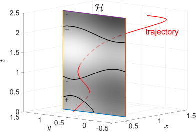
Figure 4: Eulerian coordinates: Flux density on the extended section $\mathcal{H}$, bounded by blue, yellow, purple and brown lines. Positive flux is directed in positive $x$-direction, and the flux direction through $\mathcal{H}$ is indicated by $+/-$. Zero-level curves of flux are shown in black. Also shown is the extended pathline from Fig. 2 (red, dashed when behind the section) with three transversal crossings, two positive and one negative.

In extended Eulerian coordinates, trajectories (or, extended path lines) take the form $(t,\varphi_{0}^{t}(p))$; in extended Lagrangian coordinates, trajectories are simply vertical lines, i.e., $t\mapsto(t,p)$, since they track the same particle $p$, see Fig. 5. Intersections of path lines with $\mathcal{H}$ correspond one-to-one with intersections of $\mathcal{S}$ with vertical lines.

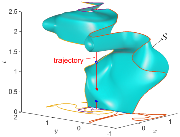
Figure 5: Lagrangian coordinates: Streak surface $\mathcal{S}$ and trajectory (red), which crosses $\mathcal{S}$ twice in positive (blue balls) and once in negative (red ball) direction. The boundary curves correspond to the boundary curves in Fig. 4 with the respective colors. Their projections onto the $t=0$ time slice are shown in the corresponding colors, cf., Fig. 2.

In a second step, we project spacetime points to their spatial coordinates by the canonical projection $\Pi\colon\mathcal{T}\times\mathbb{R}^{n}\to\mathbb{R}^{n}$ and introduce $\mathcal{D}\coloneqq\Pi(\mathcal{S})$. We view the image of $\Pi$ as the initial time slice of the extended state space and therefore parametrized by Lagrangian coordinates. By construction, we have for $\Psi\coloneqq\Pi\circ\Phi$ the identity $\Psi(t,x)=\varphi_{t}^{0}(x)$, and it is exactly the particles from $\mathcal{D}$ that cross $\mathcal{C}$ within $\mathcal{T}$ one way or another, possibly multiple times.

For later reference, we emphasize the following observation. Let $\boldsymbol{e}_{t}$ be the unit time-like vector field. Then we have

$$\mathrm{d}\phi_{0}^{t}\mathrm{d}\Psi(t,x)\boldsymbol{e}_{t}(x) =-\boldsymbol{u}_{t}(x).$$ (5a)

On the other hand, for any space-like vector field $$\boldsymbol{v}_{t} \boldsymbol{u}$$ such as, for instance, the velocity field , we have

$$\mathrm{d}\phi_{0}^{t}\mathrm{d}\Psi(t,x)\boldsymbol{v}_{t}(x) =\boldsymbol{v}_{t}(x),$$ (5b)

since in this case $\mathrm{d}\Psi$ acts like $\mathrm{d}\phi_{t}^{0}$.

4.2 Counting net crossings – the degree

We study the differentiable map $\Psi$ as a map between the two $n$-dimensional manifolds $\mathcal{H}\subset\mathcal{T}\times\mathbb{R}^{n}$ and $\mathcal{D}\subset\mathbb{R}^{n}$. To this end, we recall notions from differential topology and interpret them in our setting.

First, regular points $\left(t,x\right)\in\mathcal{H}$ are those for which the differential $\mathrm{d}\Psi(t,x)$ is invertible. This is exactly the case, when the tangent space at $\Phi(t,x)=(t,\phi_{t}^{0}(x))$ to $\mathcal{S}$ does not contain the vertical time direction. Non-regular points $(t,x)$ of $\Psi$ are referred to as critical points, which are characterized by non-transversal crossings, i.e., instantaneous stagnation points $\boldsymbol{u}_{t}(x)=0$, or tangential crossing/rebound.

According to Sard’s theorem, the set of critical values, i.e., images of critical points, has measure zero in $\mathcal{D}$, even though the set of critical points may be large in $\mathcal{H}$. Consistently, critical points do not contribute to the Eulerian flux integral.

In the Eulerian setting, positive/negative crossings of a Lagrangian particle $p$ through $\mathcal{C}$ correspond to $\pm\boldsymbol{u}_{t}(x)\boldsymbol{\cdot}\boldsymbol{n}(x)>0$ at corresponding intersections $(t,x)$. In the Lagrangian setting, positive/negative crossings are equivalent to crossings of the vertical line over $p$ through $\mathcal{S}$ from below/above with respect to the orientation on $\mathcal{S}$, see Fig. 5. This is formalized by $\pm\det\mathrm{d}\Psi>0$, which geometrically means that $\mathrm{d}\Psi(t,x)$ is orientation-preserving or orientation-reversing at the respective crossings of $p$. This is well-defined at all crossings exactly for particles $p$ which are regular values of $\Psi$.

The difference of positive and negative crossings, or, in other words, the net number of crossings, is given by the degree of $\Psi$ at $p\in\mathcal{D}$,

$$\deg\left(\Psi,p\right)\coloneqq\sum_{(t,x)\in\Psi^{-1}(p)\cap\mathcal{H}}\operatorname{sign}\left(\det\left(\mathrm{d}\Psi(t,x)\right)\right).$$

The degree function is locally constant, and can be used to define a partition of the set of particles, up to the measure-zero set of critical values. Specifically, we define $\mathcal{D}_{k}$ as the set of regular values $p$ of $\Psi$ such that $\deg\left(\Psi,p\right)=k$ for $k\in\mathbb{Z}$. Following [41], we refer to the $\mathcal{D}_{k}$’s as donating regions of fluxing index $k$. By construction, each $\mathcal{D}_{k}$ contains the particles with only transversal crossings of which there are $k$ net. In particular, all material points that do not cross $\mathcal{C}$ within $\mathcal{T}$ are contained in $\mathcal{D}_{0}$.

4.3 Area formula

In the homogeneous case $f\equiv 1$, we have the following identity for the degree of $\Psi$ [12, Section 3.1.5, Thm. 6], which is a consequence of the area formula ([8] and [19, Thm. 5.3.7]):

$$\int_{\mathcal{H}}\det\mathrm{d}\Psi(t,x)\,\mathrm{d}x\,\mathrm{d}t =\int_{\mathbb{R}^{n}}\deg(\Psi,p)\,\mathrm{d}p=\sum_{k\in\mathbb{Z}}\thinspace k\operatorname{vol}(\mathcal{D}_{k}).$$

The area formula is a generalization of the change of variables (in integral) formula to non-injective maps such as $\Psi$. Clearly, the degree measures the non-injectivity, and is equal to $\pm 1$ globally for orientation-preserving and -reversing diffeomorphisms, respectively.

Inhomogeneous conserved quantities are constant along trajectories in volume-preserving flows. Therefore, we have $f_{t}(x)=f_{0}(\Psi(t,x))$, and we conclude with the general area formula:

$$\int_{\mathcal{H}}f_{t}(x)\det\mathrm{d}\Psi(t,x)\,\mathrm{d}x\,\mathrm{d}t=\int_{\mathcal{H}}f_{0}(\Psi(t,x))\det\mathrm{d}\Psi(t,x)\,\mathrm{d}x\,\mathrm{d}t=\sum_{k}\thinspace k\int_{\mathcal{D}_{k}}f_{0}(p)\,\mathrm{d}p.$$

To prove Eq. (1) and thereby solve Problem 1, it remains to show

$$\det\mathrm{d}\Psi(t,x)=\boldsymbol{u}_{t}(x)\boldsymbol{\cdot}\boldsymbol{n}(x),$$ (6)

which is done in Appendix Section A, taking advantage of the relation (4) between the streak vector field and the velocity field.

4.4 The two-dimensional case

Our results for volume-preserving flows on $\mathbb{R}^{n}$ simplify in the two-dimensional case considered by Zhang [40, 41] as follows. It is well-known that, in our context, the degree of $\Psi$ at some regular value $p\in\mathcal{D}\subset\mathbb{R}^{2}$ equals the winding number of $p$ with respect to the closed curve $\Psi(\partial\mathcal{H})$ around $p$ [5, Section 6.6]. The winding number counts the net number of turns of $\Psi(\partial\mathcal{H})$ around $p$ under one counter-clockwise passage through $\partial\mathcal{H}$, see Fig. 2.

In the 2D case, we find the donating regions $\mathcal{D}_{k}$ of fluxing index $k$ as follows. The boundary $\partial\mathcal{H}$ of the extended section $\mathcal{H}$ is a closed curve, just as its image under $\Psi$. In Figs. 5 and 2 its image corresponds to the concatenation of the section (blue), one streakline (say, yellow), the backward image of the section (purple) and the other streakline (brown). This closed curve gives rise to possibly several connected components, simple loops, through its self-intersections. Now, the winding number is constant on the interior of each simple loop, and it suffices to compute the winding number for some contained sample point, which is a standard task in computational geometry. As anticipated in Section 2, in the case of constant density the Lagrangian flux calculation reduces to the computation of the enclosed area of each component, multiplication by its winding number and final summation over the loops.

In summary, we have generalized the main result of [41], in which only the issue of counting net crossings was treated under additional assumptions from a different methodological perspective. Note also that for the isolated counting aspect, our characterization in terms of $\deg\left(\Psi\right)$, or winding number in 2D, is also valid in the case of a compressible velocity field $\boldsymbol{u}$.

5 Moving surfaces

To find a Lagrangian flux integral in the moving surface case, Problem 2, we may proceed as in Section 4 with $\mathcal{H}=\mathcal{T}\times\mathcal{C}$ replaced by $\mathcal{H}=\bigcup_{t}\mathcal{C}_{t}$ as the domain of the maps $\Phi$ and $\Psi$. All constructions and arguments work just as well as before. It remains to find an expression analogous to Eq. (6) for $\det\mathrm{d}\Psi(t,x)$:

$$\det\mathrm{d}\Psi(t,x)=\hat{\boldsymbol{u}}_{t}(x)\boldsymbol{\cdot}\hat{\boldsymbol{n}}_{t}(x),$$

which is shown in Appendix Section B.

6 Conclusion

In this work we have devised a Lagrangian approach to transport through (codimension-one) surfaces in general $n$-dimensional, unsteady, volume-preserving flows. Studying the change from Lagrangian to Eulerian coordinates (and vice versa) alone, we have (i) discovered a striking analogy between path lines and streak lines, (ii) derived an algebraic relation between their associated velocity fields, (iii) found a natural way of determining the net number of surface crossings for individual Lagrangian particles up to a measure zero set, and, finally, (iv) transformed the Eulerian flux integral into a Lagrangian one. Thus, we have solved the donating region problem [39] for volume-preserving flows in arbitrary finite dimension and smoothly moving surfaces. An obvious extension of the methodology is to handle non-volume-preserving flows, and work is in progress in this direction.

Besides the theoretical insights, the Lagrangian approach to transport through surfaces is of major importance in at least two relevant fluid mechanical applications. First, it provides the missing theoretical foundation of a family of highly accurate semi-Lagrangian finite volume and interface tracking methods [38, 39]. Second, it facilitates the efficient computation of transport by Lagrangian coherent vortices in large-scale oceanic flows [18, 17].

Appendix A Proof of $\det\mathrm{d}\Psi=\boldsymbol{u\cdot n}$

We show that $\det\mathrm{d}\Psi(t,x)=\boldsymbol{u}_{t}(x)\boldsymbol{\cdot}\boldsymbol{n}(x)$. To this end, fix a regular point $(t,x)\in\mathcal{H}$. Then $\Psi$ acts diffeomorphically between an open neighborhood $\mathcal{U}$ of $(t,x)$ in $\mathcal{H}$ and its image $\mathcal{V}\coloneqq\Psi(\mathcal{U})$ in $\mathcal{D}$. We may choose local coordinates on $\mathcal{U}$ such that in $(t,x)$ we have an orthonormal basis, i.e., $\boldsymbol{e}_{t}\in T_{t}\mathcal{T}$, $\operatorname{span}\left\{\boldsymbol{e}_{2},\ldots,\boldsymbol{e}_{n}\right\}=T_{x}\mathcal{C}$ and $\boldsymbol{e}_{1}\in T_{x}^{\perp}\mathcal{H}$, with

$$\bigwedge_{i=1}^{n}\boldsymbol{e}_{i}=\boldsymbol{e}_{1}\wedge\ldots\wedge\boldsymbol{e}_{n},\qquad\boldsymbol{e}_{t}\wedge\boldsymbol{e}_{2}\wedge\ldots\wedge\boldsymbol{e}_{n},\qquad\text{and}\qquad\boldsymbol{e}_{t}\wedge\boldsymbol{e}_{1}\wedge\ldots\wedge\boldsymbol{e}_{n},$$

unit volume parallelepipeds. To avoid a discussion on delicate orientation issues, the following calculations involving determinants are to be read up to sign. To avoid notational clutter, we use the $\wedge$-notation to denote both the spanned parallelepipeds and their volume, computed as the determinant of the matrix with columns given by the factors of the wedge product.

On the one hand, we have

$$\boldsymbol{u}_{t}\boldsymbol{\cdot}\boldsymbol{n}=\boldsymbol{u}_{t}\boldsymbol{\cdot}\boldsymbol{e}_{1}=\det\begin{pmatrix}|&|&&|\\ \boldsymbol{u}_{t}&\boldsymbol{e}_{2}&\cdots&\boldsymbol{e}_{n}\\ |&|&&|\end{pmatrix}=\boldsymbol{u}_{t}\wedge\boldsymbol{e}_{2}\wedge\cdots\wedge\boldsymbol{e}_{n}=\boldsymbol{u}_{t}\wedge\bigwedge_{i=2}^{n}\boldsymbol{e}_{i}.$$

On the other hand, we first observe that

$$\det\left(\mathrm{d}\varphi_{0}^{t}\mathrm{d}\Psi\bigr{|}_{(t,x)}\right)=\det\mathrm{d}\varphi_{0}^{t}\det\mathrm{d}\Psi\bigr{|}_{(t,x)}=\det\mathrm{d}\Psi\bigr{|}_{(t,x)},$$ (7)

since $\det\mathrm{d}\varphi_{0}^{t}=1$ for all $t$. Finally, we compute $\det\left(\mathrm{d}\varphi_{0}^{t}\mathrm{d}\Psi\bigr{|}_{(t,x)}\right)$ as the change of volume under the action of $\mathrm{d}\varphi_{0}^{t}\mathrm{d}\Psi\bigr{|}_{(t,x)}$:

$$\frac{\left(\mathrm{d}\varphi_{0}^{t}\mathrm{d}\Psi\bigr{|}_{(t,x)}\boldsymbol{e}_{t}\right)\wedge\bigwedge_{i=2}^{n}\left(\mathrm{d}\varphi_{0}^{t}\mathrm{d}\Psi\bigr{|}_{(t,x)}\boldsymbol{e}_{i}\right)}{\boldsymbol{e}_{t}\wedge\boldsymbol{e}_{2}\wedge\ldots\wedge\boldsymbol{e}_{n}}=\mathrm{d}\varphi_{0}^{t}\boldsymbol{w}_{t}\wedge\bigwedge_{i=2}^{n}\boldsymbol{e}_{i}=\boldsymbol{u}_{t}\wedge\bigwedge_{i=2}^{n}\boldsymbol{e}_{i},$$

where we have used Eqs. (4) and (5). With Eq. (7), this finishes the proof.

Appendix B Proof of $\det\mathrm{d}\Psi=\hat{\boldsymbol{u}}\boldsymbol{\cdot}\hat{\boldsymbol{n}}$

We choose a local unit volume tangent space basis as in Section A. The tangent space $T_{(t,x)}\mathcal{H}$ is then spanned by the orthogonal basis $\left(\boldsymbol{e}_{t}+\beta\boldsymbol{e}_{1},\boldsymbol{e}_{2},\ldots,\boldsymbol{e}_{n}\right)$. With $\alpha=\lVert\boldsymbol{e}_{t}+\beta\boldsymbol{e}_{1}\rVert=\sqrt{1+\beta^{2}}$, we have that $\frac{1}{\alpha}(\boldsymbol{e}_{t}+\beta\boldsymbol{e}_{1})\wedge\boldsymbol{e}_{2}\wedge\ldots\wedge\boldsymbol{e}_{n}$ is a unit $n$-volume parallelepiped in $T_{(t,x)}\mathcal{H}$.

Next, we calculate $\det\left(\mathrm{d}\phi_{0}^{t}\mathrm{d}\Psi\right)$ as the change of volume under $\mathrm{d}\phi_{0}^{t}\mathrm{d}\Psi\bigr{|}_{(t,x)}$:

$$\det\left(\mathrm{d}\phi_{0}^{t}\mathrm{d}\Psi\bigr{|}_{(t,x)}\right) =\frac{\left(\frac{1}{\alpha}\mathrm{d}\phi_{0}^{t}\mathrm{d}\Psi\bigr{|}_{(t,x)}(\boldsymbol{e}_{t}+\beta\boldsymbol{e}_{1})\right)\wedge\bigwedge_{i=2}^{n}\mathrm{d}\phi_{0}^{t}\mathrm{d}\Psi\bigr{|}_{(t,x)}\boldsymbol{e}_{i}}{\frac{1}{\alpha}(\boldsymbol{e}_{t}+\beta\boldsymbol{e}_{1})\wedge\boldsymbol{e}_{2}\wedge\ldots\wedge\boldsymbol{e}_{n}}$$

$$=\tfrac{1}{\alpha}(\boldsymbol{u}_{t}(x)-\beta\boldsymbol{e}_{1})\wedge\boldsymbol{e}_{2}\wedge\ldots\wedge\boldsymbol{e}_{n}$$

$$=\tfrac{1}{\alpha}(\boldsymbol{u}_{t}(x)-\beta\boldsymbol{e}_{1})\boldsymbol{\cdot}\boldsymbol{n}.$$

From the first to the second line, we have used that the denominator is normalized, and the different signs are due to Eq. (5).

On the other hand, let us calculate the $\hat{\boldsymbol{n}}$-component of the extended velocity $\hat{\boldsymbol{u}}_{t}=\boldsymbol{e}_{t}+\boldsymbol{u}_{t}$, i.e., the component normal to the section’s tangent space $T_{(t,x)}\mathcal{H}$:

$$(\boldsymbol{e}_{t}+\boldsymbol{u}_{t})\boldsymbol{\cdot}\hat{\boldsymbol{n}} =(\boldsymbol{e}_{t}+\boldsymbol{u}_{t})\wedge\tfrac{1}{\alpha}(\boldsymbol{e}_{t}+\beta\boldsymbol{e}_{1})\wedge\boldsymbol{e}_{2}\wedge\ldots\wedge\boldsymbol{e}_{n}$$

$$=\tfrac{1}{\alpha}\boldsymbol{e}_{t}\wedge(\boldsymbol{u}_{t}-\beta\boldsymbol{e}_{1})\wedge\boldsymbol{e}_{2}\wedge\ldots\wedge\boldsymbol{e}_{n}$$

$$=\tfrac{1}{\alpha}(\boldsymbol{u}_{t}-\beta\boldsymbol{e}_{1})\wedge\boldsymbol{e}_{2}\wedge\ldots\wedge\boldsymbol{e}_{n}$$

$$=\tfrac{1}{\alpha}(\boldsymbol{u}_{t}(x)-\beta\boldsymbol{e}_{1})\boldsymbol{\cdot}\boldsymbol{n}.$$

From the first to the second line, we have used determinant rules, and from the second to the third lines Laplace expansion along the time component.

Finally, the above calculation is, of course, consistent with the one given in Section A, since $\boldsymbol{u}\boldsymbol{\cdot}\boldsymbol{n}=\hat{\boldsymbol{u}}\boldsymbol{\cdot}\hat{\boldsymbol{n}}$ whenever $\hat{\boldsymbol{n}}=\left(\begin{smallmatrix}0\\ \boldsymbol{n}\end{smallmatrix}\right)$, i.e., when the section does not move. In this case, $\beta=0$ and $\alpha=1$.

References

- [1] S. Balasuriya. Cross-separatrix flux in time-aperiodic and time-impulsive flows. Nonlinearity, 19(12):2775, 2006. doi:10.1088/0951-7715/19/12/003.
- [2] G. K. Batchelor. An Introduction to Fluid Dynamics. Cambridge Mathematical Library. Cambridge University Press, 2000. doi:10.1017/CBO9780511800955.
- [3] A. H. Boozer. Physics of magnetically confined plasmas. Rev. Mod. Phys., 76:1071–1141, 2005. doi:10.1103/RevModPhys.76.1071.
- [4] W. M. Deen. Analysis of transport phenomena. Oxford University Press, 2 edition, 2013.
- [5] K. Deimling. Nonlinear Functional Analysis. Springer, 1985. doi:10.1007/978-3-662-00547-7.
- [6] C. Dong, J. C. McWilliams, Y. Liu, and D. Chen. Global heat and salt transports by eddy movement. Nature Communications, 5(3294):1–6, 2014. doi:10.1038/ncomms4294.
- [7] A. K. M. Fazle Hussain. Coherent structures and turbulence. J. Fluid Mech., 173:303–356, 1986. doi:10.1017/S0022112086001192.
- [8] H. Federer. Geometric Measure Theory. Classics in Mathematics. Springer, 1996. doi:10.1007/978-3-642-62010-2.
- [9] G. Froyland. An analytic framework for identifying finite-time coherent sets in time-dependent dynamical systems. Physica D, 250(0):1 – 19, 2013. doi:10.1016/j.physd.2013.01.013.
- [10] G. Froyland. Dynamic isoperimetry and the geometry of Lagrangian coherent structures. Nonlinearity, 28(10):3587–3622, 2015. doi:10.1088/0951-7715/28/10/3587.
- [11] G. Froyland and K. Padberg-Gehle. A rough-and-ready cluster-based approach for extracting finite-time coherent sets from sparse and incomplete trajectory data. Chaos, 25(8):087406–, 2015. doi:10.1063/1.4926372.
- [12] M. Giaquinta, G. Modica, and J. Souček. Cartesian Currents in the Calculus of Variations I: Cartesian Currents, volume 37 of Ergebnisse der Mathematik und ihrer Grenzgebiete. Springer, 1998.
- [13] A. Hadjighasem, D. Karrasch, H. Teramoto, and G. Haller. A Spectral Clustering Approach to Lagrangian Vortex Detection. 2015. submitted. arXiv:1506.02258.
- [14] G. Haller. Langrangian Coherent Structures. Annu. Rev. Fluid Mech., 47(1):137–161, 2015. doi:10.1146/annurev-fluid-010313-141322.
- [15] G. Haller and F. J. Beron-Vera. Coherent Lagrangian vortices: the black holes of turbulence. J. Fluid Mech., 731:R4, 2013. doi:10.1017/jfm.2013.391.
- [16] M. W. Hirsch. Differential Topology. Springer, 1976. doi:10.1007/978-1-4684-9449-5.
- [17] F. Huhn, M. Mazloff, T. Schneider, and G. Haller. Coherent Lagrangian eddies and coherent transport in the Agulhas leakage. 2015. in preparation.
- [18] D. Karrasch, F. Huhn, and G. Haller. Automated detection of coherent Lagrangian vortices in two-dimensional unsteady flows. Proc. R. Soc. A, 471(2173):20140639, 2015. doi:10.1098/rspa.2014.0639.
- [19] S. G. Krantz and H. Parks. Geometric Integration Theory. Cornerstones. Birkhäuser, 2008. doi:10.1007/978-0-8176-4679-0.
- [20] J. Lin, D. Brunner, C. Gerbig, A. Stohl, A. Luhar, P. Webley, and editors. Lagrangian Modeling of the Atmosphere, volume 200 of Geophysical Monograph Series. American Geophysical Union, 2013. doi:10.1029/GM200.
- [21] T. Ma and E. M. Bollt. Differential Geometry Perspective of Shape Coherence and Curvature Evolution by Finite-Time Non-hyperbolic Splitting. SIAM J. Appl. Dyn. Syst., 13(3):1106–1136, 2014. doi:10.1137/130940633.
- [22] R. S. MacKay. Transport in 3D volume-preserving flows. J. Nonlinear Sci., 4(1):329–354, 1994. doi:10.1007/BF02430637.
- [23] R. S. MacKay, J. D. Meiss, and I. C. Percival. Transport in Hamiltonian systems. Physica D, 13(1-2):55–81, 1984. doi:10.1016/0167-2789(84)90270-7.
- [24] R.S. MacKay. Flux over a saddle. Phys. Lett. A, 145(8,9):425 – 427, 1990. doi:10.1016/0375-9601(90)90306-9.
- [25] N. Malhotra and S. Wiggins. Geometric Structures, Lobe Dynamics, and Lagrangian Transport in Flows with Aperiodic Time-Dependence, with Applications to Rossby Wave Flow. Journal of Nonlinear Science, 8(4):401–456, 1998. doi:10.1007/s003329900057.
- [26] J. C. McWilliams. The emergence of isolated coherent vortices in turbulent flow. J. Fluid Mech., 146:21–43, 1984. doi:10.1017/S0022112084001750.
- [27] J. W. Milnor. Topology from the Differentiable Viewpoint. The University Press of Virginia, 1965.
- [28] B. A. Mosovsky, M. F. M. Speetjens, and J. D. Meiss. Finite-Time Transport in Volume-Preserving Flows. Phys. Rev. Lett., 110(21):214101, 2013. doi:10.1103/PhysRevLett.110.214101.
- [29] R. Mundel, E. Fredj, H. Gildor, and V. Rom-Kedar. New Lagrangian diagnostic for characterizing fluid flow mixing. Phys. Fluids, 26:126602, 2014. doi:10.1063/1.4903239.
- [30] J. M. Ottino. The Kinematics of Mixing: Stretching, Chaos, and Transport. Cambridge University Press, 1989.
- [31] Z. Pouransari, M. F. M. Speetjens, and H. J. H. Clercx. Formation of coherent structures by fluid inertia in three-dimensional laminar flows. J. Fluid Mech., 654:5–34, 7 2010. doi:10.1017/S0022112010001552.
- [32] A. Provenzale. Transport by Coherent Barotropic Vortices. Annu. Rev. Fluid Mech., 31(1):55–93, 1999. doi:10.1146/annurev.fluid.31.1.55.
- [33] V. Rom-Kedar and S. Wiggins. Transport in two-dimensional maps. Arch. Ration. Mech. Anal., 109:239–298, 1990. doi:10.1007/BF00375090.
- [34] R. M. Samelson and S. Wiggins. Lagrangian Transport in Geophysical Jets and Waves, volume 31 of Interdisciplinary Applied Mathematics. Springer, 2006. doi:10.1007/978-0-387-46213-4.
- [35] M. F. M. Speetjens, E. A. Demissie, G. Metcalfe, and H. J. H. Clercx. Lagrangian transport characteristics of a class of three-dimensional inline-mixing flows with fluid inertia. Phys. Fluids, 26(11):113601, 2014. doi:10.1063/1.4901822.
- [36] T. Weinkauf and H. Theisel. Streak Lines as Tangent Curves of a Derived Vector Field. Visualization and Computer Graphics, IEEE Transactions on, 16(6):1225–1234, 2010. doi:10.1109/TVCG.2010.198.
- [37] S. Wiggins. Chaotic Transport in Dynamical Systems, volume 2 of Interdisciplinary Applied Mathematics. Springer, 1992. doi:10.1007/978-1-4757-3896-4.
- [38] Q. Zhang. Highly accurate Lagrangian flux calculation via algebraic quadratures on spline-approximated donating regions. Comput. Methods Appl. Mech. Engrg., 264:191–204, 2013. doi:10.1016/j.cma.2013.05.024.
- [39] Q. Zhang. On a Family of Unsplit Advection Algorithms for Volume-of-Fluid Methods. SIAM J. Numer. Anal., 51(5):2822–2850, 2013. doi:10.1137/120897882.
- [40] Q. Zhang. On Donating Regions: Lagrangian Flux through a Fixed Curve. SIAM Review, 55(3):443–461, 2013. doi:10.1137/100796406.
- [41] Q. Zhang. On generalized donating regions: Classifying Lagrangian fluxing particles through a fixed curve in the plane. J. Math. Anal. Appl., 424(2):861–877, 2015. doi:10.1016/j.jmaa.2014.11.043.
- [42] Z. Zhang, W. Wang, and B. Qiu. Oceanic mass transport by mesoscale eddies. Science, 345(6194):322–324, 2014. doi:10.1126/science.1252418.