Renewal Approach to the Analysis of the Asynchronous State for Coupled Noisy Oscillators

Abstract

We develop a framework in which the activity of nonlinear pulse-coupled oscillators is posed within the renewal theory. In this approach, the evolution of inter-event density allows for a self-consistent calculation that determines the asynchronous state and its stability. This framework, can readily be extended to the analysis of systems with more state variables. To exhibit this, we study a nonlinear pulse-coupled system, where couplings are dynamic and activity dependent. We investigate stability of this system and we show it undergoes a super-critical Hopf bifurcation to collective synchronization.

The collective dynamics of pulse-coupled networks of nonlinear oscillators has been studied extensively kuramoto_chemical_2003 ; *winfree_geometry_2001. In the presence of noise, the approach has been to analyze the Fokker-Planck equation of the state variables of the oscillators. This has been highly successful for systems with units described by a single variable. However, it has proven to be difficult to extend this approach to systems with several state variables. This is because in such systems the Fokker-Planck equation may have a highly non-trivial boundary conditions risken_fokker-planck_1996 . An other long standing theoretical framework to study irregularly pulsing units is the theory of the stochastic point processes. In this theory, the event times are described by probability density functions which are history dependent. Solutions of the first passage time problem have long been used to connect this phenomenological description to the underlying dynamics of the state variables schrodinger_zur_1915 ; *chandrasekhar_dynamical_1943; *wang_theory_1945.

In this letter, we marry these two approaches, exploiting the fact in that pulse-coupled systems the recurrent inputs into the units is fully determined by the timing of events. The only element that needs to be added to the first passage time description, is the self-consistency of the interactions and the network output. We first demonstrate our method on a simple system and show that the description of asynchronous state and its stability is consistent with previously derived results abbott_asynchronous_1993 ; brunel_sparsely_2008 . We then add a dynamic component to the interactions. This addition is not readily incorporated within the Fokker-Plank approach, however, it is easily incorporated in our formalism. Such dynamic recurrent couplings can be observed in many physical systems. For instance, temporal dynamics of intracellular signaling activities is tightly regulated by positive or negative feedback kholodenko_cell-signalling_2006 , similarly biochemical processes concerning transmitter production and release in synapses in the network of neurons are known to be modulated by the activity of interacting cells grossberg_production_1969 ; tsodyks_neural_1998 .

We consider a network of $N$ identical oscillators with all-to-all feedback coupling, which receives a noisy external input. We assume that the oscillators are modeled as integrate and fire neurons, where their the membrane voltage is the state variable. Between events the (normalized) voltage $x_{i}$, of oscillator $i$ satisfies

$${\tau_{\mathrm{m}}}\frac{d}{dt}x_{i}=\iota_{i}(t)-x_{i},$$ (1)

where ${\tau_{\mathrm{m}}}$ is the membrane time constant and $\iota_{i}$ is the input current into oscillator $i$. When the voltage reaches the threshold, $x_{\mathrm{thr}}=1$, the oscillator emits a pulse and the voltage is immediately reset to the resting potential, $x_{\mathrm{r}}=0$. The input, $\iota_{i}$, can be written as $\iota_{i}=\iota_{i,{\mathrm{ext}}}+\iota_{i,{\mathrm{fb}}}$ where $\iota_{i,{\mathrm{ext}}}$ and $\iota_{i,{\mathrm{fb}}}$ are the external and feedback input respectively. The external current is given by $\iota_{i,ext}(t)=\mu_{\mathrm{ext}}+\sigma\eta_{i}(t)$, where the $\eta_{i}$s are independent Gaussian white noise variables, $\langle\eta_{i}(t)\rangle=0$ and $\langle\eta_{i}(t)\eta_{j}(t^{\prime})\rangle=\delta_{ij}(t-t^{\prime})$. When a oscillator emits a pulse at time $t_{k}$, this causes a, so-called synaptic, current input $s(t-t_{k})$ in all oscillators. This input is given by

$$s(t)=\frac{{g_{\mathrm{s}}}}{N}\frac{1}{{\tau_{\mathrm{s}1}}-{\tau_{\mathrm{s}2}}}\left(e^{-t/{\tau_{\mathrm{s}1}}}-e^{-t/{\tau_{\mathrm{s}2}}}\right)\Theta(t),$$ (2)

where $\Theta$ is the Heaviside function. Here ${\tau_{\mathrm{s}2}}$ and ${\tau_{\mathrm{s}1}}$ are the synaptic rise and decay times. We study the network in the thermodynamic limit ($N\rightarrow\infty$). In this limit the total recurrent input into all oscillators is identical, $\iota_{i,{\mathrm{fb}}}=\mu_{\mathrm{fb}}$, and is given by

$$\left(1+{\tau_{\mathrm{s}1}}\frac{d}{dt}\right)\left(1+{\tau_{\mathrm{s}2}}\frac{d}{dt}\right)\mu_{\mathrm{fb}}(t)={g_{\mathrm{s}}}r(t),$$ (3)

where $r(t)=N^{-1}\sum_{i}\sum_{k}\delta(t-t_{i,k})$ is the population firing rate. Here, $t_{i,k}$ is the time of the $k$th event of oscillator $i$.

To calculate inter-event density, we use that when oscillator $i$ emits a pulse at time ${t^{\prime}}$, we have that $x_{i}({t^{\prime}})=0$ and $x_{i}$ satisfies the stochastic differential equation ${\tau_{\mathrm{m}}}\frac{d}{dt}x_{i}=\mu(t)-x_{i}+\sigma\eta_{i}(t)$ until $x_{i}$ reaches $1$. Averaging over the realizations of the noise the probability density $\rho(x,t|{t^{\prime}})$ for $x_{i}(t)=x$ and no event has occurred between ${t^{\prime}}$ and $t$ satisfies the Fokker-Planck equation

$${\tau_{\mathrm{m}}}\frac{\partial}{\partial t}\rho(x,t|{t^{\prime}})=-\frac{\partial}{\partial x}[\mu(t)-x]\rho(x,t|{t^{\prime}})+\frac{\sigma^{2}}{2}\frac{\partial}{\partial x^{2}}\rho(x,t|{t^{\prime}}),$$ (4)

with initial condition $\rho(x,t^{\prime}|t^{\prime})=\delta(x)$ and boundary condition $\rho(1,t|t^{\prime})=0$. The difficulty in solving this is in satisfying the boundary condition. For an unrestricted process, which satisfies Eqn. (4) it is straightforward to show that with initial condition $x_{i}({t^{\prime}})={x^{\prime}}$ the probability density $\hat{\rho}(x,t|{x^{\prime}},{t^{\prime}})$ for $x_{i}(t)=x$ satisfies, for $t\geq{t^{\prime}}$

$$\hat{\rho}(x,t|{x^{\prime}},{t^{\prime}})=\frac{1}{\sqrt{2\pi}\Sigma(t-{t^{\prime}})}\exp\left(\frac{-(x-x_{\mathrm{ave}}(t|{x^{\prime}},{t^{\prime}}))^{2}}{2\Sigma^{2}(t-{t^{\prime}})}\right),$$ (5)

where the noise-averaged of $x$ is denoted as $x_{\mathrm{ave}}$ and it satisfies

$$x_{\mathrm{ave}}(t|{x^{\prime}},{t^{\prime}})={x^{\prime}}e^{-(t-{t^{\prime}})/{\tau_{\mathrm{m}}}}+\frac{1}{{\tau_{\mathrm{m}}}}\int_{{t^{\prime}}}^{t}\!d{t^{\prime\prime}}\,\mu({t^{\prime\prime}})e^{-(t-{t^{\prime\prime}})/{\tau_{\mathrm{m}}}}$$ (6)

and the variance $\Sigma^{2}$ is given by

$$\Sigma^{2}(t)=\frac{\sigma^{2}}{2{\tau_{\mathrm{m}}}}\left[1-e^{-2t/{\tau_{\mathrm{m}}}}\right].$$ (7)

The problem with initial condition $\rho(x,{t^{\prime}}|{t^{\prime}})=\delta(x)$ and an absorbing boundary at $x=1$ can be viewed as an unrestricted process, where a particle is inserted at $x=0$ at time ${t^{\prime}}$ and extracted at $x=1$ at time $t$ with some probability density ${\Pr}(t|{t^{\prime}})$ so that

$$\rho(x,t|{t^{\prime}})=\hat{\rho}(x,t|0,{t^{\prime}})-\int_{{t^{\prime}}}^{t}\!d{t^{\prime\prime}}\,{\Pr}({t^{\prime\prime}}|{t^{\prime}})\hat{\rho}(x,t|1,{t^{\prime\prime}}).$$ (8)

The inter-event probability density ${\Pr}(t|{t^{\prime}})$ is determined by the boundary condition, $\rho(1,t|{t^{\prime}})=0$ and thus satisfies the Volterra integral equation

$$\hat{\rho}(1,t|0,{t^{\prime}})=\int_{{t^{\prime}}}^{t}\!d{t^{\prime\prime}}\,\hat{\rho}(1,t|1,{t^{\prime\prime}}){\Pr}({t^{\prime\prime}}|{t^{\prime}}).$$ (9)

In the asynchronous state the emission rate is constant, $r(t)=r_{\mathrm{eq}}$, and we have $\mu(t)=\mu_{\mathrm{eq}}=\mu_{\mathrm{ext}}+g_{s}r_{\mathrm{eq}}$. Consequently, $\hat{\rho}$ is given by $\hat{\rho}(x,t|{x^{\prime}},{t^{\prime}})=\hat{\rho}_{\mathrm{eq}}(x,t-{t^{\prime}}|{x^{\prime}})$, where $\hat{\rho}_{\mathrm{eq}}(x,t|{x^{\prime}})$ satisfies Eqn. (5) with $x_{\mathrm{ave}}(t|{x^{\prime}},{t^{\prime}})=x_{\mathrm{ave,eq}}(t-{t^{\prime}}|{x^{\prime}})=\mu_{\mathrm{eq}}+({x^{\prime}}-\mu_{\mathrm{eq}})\exp(-[t-{t^{\prime}}]/{\tau_{\mathrm{m}}})$. Note that for $t\rightarrow\infty$, $\hat{\rho}_{\mathrm{eq}}(x,t|{x^{\prime}})\rightarrow\hat{\rho}_{\infty}(x)\equiv\exp(-(x-\mu_{\mathrm{eq}})^{2}/2\Sigma_{\infty}^{2})/\sqrt{2\pi}\Sigma_{\infty}$, where $\Sigma_{\infty}=\sigma/\sqrt{2{\tau_{\mathrm{m}}}}$, Additionally, the inter-event probability density can be written as ${\Pr}(t|{t^{\prime}})={\Pr}_{\mathrm{eq}}(t-{t^{\prime}})$ as this density is time invariant in the stationary asynchronous regime. This density must satisfy the following Volterra integral equation

$$\hat{\rho}_{\mathrm{eq}}(1,t|0)=\int_{0}^{t}\!d{t^{\prime}}\hat{\rho}_{\mathrm{eq}}(1,t-{t^{\prime}}|1){\Pr}_{\mathrm{eq}}({t^{\prime}}).$$ (10)

The right hand side of this equation is now a convolution and this can be solved using the Laplace transform. The Laplace transform ${\Pr}_{\mathrm{eq},\mathrm{L}}$ of ${\Pr}_{\mathrm{eq}}$ satisfies

$${\Pr}_{\mathrm{eq},\mathrm{L}}(s)=\frac{\hat{\rho}_{\mathrm{eq},\mathrm{L}}(1,s|0)}{\hat{\rho}_{\mathrm{eq},\mathrm{L}}(1,s|1)},$$ (11)

where $\hat{\rho}_{\mathrm{eq},\mathrm{L}}$ is the Laplace transform of $\hat{\rho}_{\mathrm{eq}}$. In the supplementary material [Supplementarymatrialat]supp, we show that the Laplace transform of Ornstein-Uhlenbeck density $\hat{\rho}_{\mathrm{eq},\mathrm{L}}$, can be formally calculated (for an alternative derivation refer to tuckwell_introduction_2005 ). Now, we can close the system, since the average inter-event interval, $\langle t\rangle$, can be found using $\langle t\rangle=-{\lim}_{s\rightarrow 0}d{\Pr}_{\mathrm{eq},\mathrm{L}}(s)/ds$ and this allows to express $r_{\mathrm{eq}}=1/\langle t\rangle$ in terms of $\mu_{\mathrm{eq}}$ and $\sigma$, together with $\mu_{\mathrm{eq}}=\mu_{ext}+g_{s}r_{\mathrm{eq}}$ that determines $r_{\mathrm{eq}}$.

To determine the stability of the asynchronous state we consider the evolution of small perturbations around the equilibrium firing rate, $r(t)=r_{\mathrm{eq}}+\epsilon r_{1}(t)$. With such a perturbation the noise averaged input into oscillators $\mu(t)$ satisfies $\mu(t)=\mu_{\mathrm{eq}}+\epsilon\mu_{1}(t)$, where $\mu_{1}$ is given by

$$\mu_{1}(t)={g_{\mathrm{s}}}\frac{1}{{\tau_{\mathrm{s}1}}-{\tau_{\mathrm{s}2}}}\int_{0}^{\infty}\!d{t^{\prime}}\,r_{1}(t-{\tau_{\mathrm{d}}}-{t^{\prime}})(e^{-{t^{\prime}}/{\tau_{\mathrm{s}1}}}-e^{-{t^{\prime}}/{\tau_{\mathrm{s}2}}}).$$ (12)

The probability density $\hat{\rho}$ for the unconstrained diffusion still satisfies Eqn. (5), but now with $\bar{x}(t|{x^{\prime}},{t^{\prime}})=\bar{x}_{\mathrm{eq}}(t-{t^{\prime}}|{x^{\prime}})+\epsilon\bar{x}_{1}(t|{t^{\prime}})$, where $\bar{x}_{1}$ satisfies

$$\bar{x}_{1}(t|{t^{\prime}})=\int_{{t^{\prime}}}^{t}\!d{t^{\prime\prime}}\mu_{1}({t^{\prime\prime}})e^{-(t-{t^{\prime\prime}})/{\tau_{\mathrm{m}}}}.$$ (13)

Thus, we can expand $\hat{\rho}$ as $\hat{\rho}(x,t|{x^{\prime}},{t^{\prime}})=\hat{\rho}_{\mathrm{eq}}(x,t-{t^{\prime}}|{x^{\prime}})+\epsilon\hat{\rho}_{1}(x,t|{x^{\prime}},{t^{\prime}})+O(\epsilon^{2})$, where

$$\hat{\rho}_{1}(x,t|{x^{\prime}},{t^{\prime}})=-\bar{x}_{1}(t|{t^{\prime}})\frac{\partial}{\partial x}\hat{\rho}(x,t-{t^{\prime}}|{x^{\prime}}).$$ (14)

Next, we write for the inter-events probability density ${\Pr}(t|{t^{\prime}})={\Pr}_{\mathrm{eq}}(t-{t^{\prime}})+\epsilon{\Pr}_{1}(t|{t^{\prime}})+O(\epsilon^{2})$ and insert this with the expansion for $\hat{\rho}$ in Eqn. (9), to obtain for ${\Pr}_{1}(t|{t^{\prime}})$ the Volterra integral equation

$$\hat{\rho}_{1}(1,t|0,{t^{\prime}}) - \int_{{t^{\prime}}}^{t}\!d{t^{\prime\prime}}\,\hat{\rho}_{1}(1,t|0,{t^{\prime\prime}}){\Pr}_{\mathrm{eq}}({t^{\prime\prime}}-{t^{\prime}})$$ (15)

$$= \int_{{t^{\prime}}}^{t}\!d{t^{\prime\prime}}\,\hat{\rho}_{\mathrm{eq}}(1,t-{t^{\prime\prime}}|0){\Pr}_{1}({t^{\prime\prime}}|{t^{\prime}}).$$

Finally, we close the system using $r(t)$, that is

$$r_{\mathrm{eq}}+\epsilon r_{1}(t)=\int_{-\infty}^{t}\!d{t^{\prime}}\,[{\Pr}_{\mathrm{eq}}(t|{t^{\prime}})+\epsilon{\Pr}_{1}(t|{t^{\prime}})][r_{\mathrm{eq}}+\epsilon r_{1}({t^{\prime}})]+O(\epsilon^{2}).$$ (16)

For sufficiently small $\epsilon$, we can ignore terms of order $\epsilon^{2}$. In this linearized system, we can make the usual Ansatz that $r_{1}(t)=r_{\lambda}e^{\lambda t}$. With this Ansatz we will, as we will see below, have $\mu_{1}(t)=r_{\lambda}e^{\lambda t}\mu_{\lambda}$, $\hat{\rho}_{1}(x,t|{x^{\prime}},{t^{\prime}})=r_{\lambda}e^{\lambda t}\hat{\rho}_{\lambda}(x,t-{t^{\prime}}|{x^{\prime}})$ and ${\Pr}_{1}(t|{t^{\prime}})=r_{\lambda}e^{\lambda t}{\Pr}_{\lambda}(t-{t^{\prime}})$. Inserting this in Eqn. (16) we obtain the eigenvalue equation

$$\int_{0}^{\infty}\!dt\,{\Pr}_{\mathrm{eq}}(t)e^{-\lambda t}+r_{\mathrm{eq}}\int_{0}^{\infty}\!dt\,{\Pr}_{\lambda}(t)=1.$$ (17)

With $r_{1}(t)=r_{\lambda}e^{-\lambda t}$ we have

$$\mu_{1}=r_{\lambda}e^{-\lambda t}\frac{{g_{\mathrm{s}}}e^{-\lambda{\tau_{\mathrm{d}}}}}{(1+\lambda{\tau_{\mathrm{s}1}})(1+\lambda{\tau_{\mathrm{s}2}})}$$ (18)

and

$$\bar{x}_{1}(t|{x^{\prime}},{t^{\prime}})=r_{\lambda}e^{-\lambda t}A_{\lambda}(t,{t^{\prime}}),$$ (19)

where $A_{\lambda}(t,{t^{\prime}})=\frac{{g_{\mathrm{s}}}e^{-\lambda{\tau_{\mathrm{d}}}}(1-e^{-(\lambda+1/{\tau_{\mathrm{m}}})(t-{t^{\prime}})})}{(1+\lambda{\tau_{\mathrm{s}1}})(1+\lambda{\tau_{\mathrm{s}2}})(1+\lambda{\tau_{\mathrm{m}}})}$. Thus, we can write $\hat{\rho}_{1}$ as $\hat{\rho}_{1}(x,t|{x^{\prime}},{t^{\prime}})=r_{\lambda}e^{-\lambda t}\hat{\rho}_{\lambda}(x,t-{t^{\prime}}|{x^{\prime}})$ with

$$\hat{\rho}_{\lambda}(x,t-{t^{\prime}}|{x^{\prime}})=-A_{\lambda}(t,{t^{\prime}})\frac{\partial}{\partial x}\hat{\rho}_{\mathrm{eq}}(x,t-{t^{\prime}}|{x^{\prime}})$$ (20)

We insert this into Eqn. (15), we find hat ${\Pr}_{1}$ is given by ${\Pr}_{1}(t|{t^{\prime}})=r_{\lambda}e^{-\lambda t}{\Pr}_{\lambda}(t-{t^{\prime}})$, where ${\Pr}_{\lambda}$ satisfies

$$\int_{0}^{t}\!d{t^{\prime}}\,\hat{\rho}_{\mathrm{eq}}(1,t-{t^{\prime}}|1)e^{-\lambda(t-{t^{\prime}})}{\Pr}_{\lambda}({t^{\prime}})$$

$$=\hat{\rho}_{\lambda}(1,t|0)-\int_{0}^{t}\!d{t^{\prime}}\,\hat{\rho}_{\lambda}(1,t-{t^{\prime}}|1){\Pr}_{\mathrm{eq}}({t^{\prime}}).$$ (21)

Multiplying both sides by $e^{-st}$ and integrating over $t$ we find for the Laplace transform ${\Pr}_{\lambda\mathrm{L}}$ of ${\Pr}_{\lambda}$

$${\Pr}_{\lambda,\mathrm{L}}(s)=\frac{\hat{\rho}_{\lambda,\mathrm{L}}(1,s|0)-\hat{\rho}_{\lambda,\mathrm{L}}(1,s|1){\Pr}_{\mathrm{eq},\mathrm{L}}(s)}{\hat{\rho}_{\mathrm{eq},\mathrm{L}}(1,s+\lambda|1)}.$$ (22)

Here $\hat{\rho}_{\lambda,\mathrm{L}}$, the Laplace transform of $\hat{\rho}_{\lambda}$ that satisfies

$$\hat{\rho}_{\lambda,\mathrm{L}}(x,s|{x^{\prime}})=-\frac{\partial}{\partial x}B_{\lambda}(\hat{\rho}_{0,\mathrm{L}}(x,s|{x^{\prime}})-\hat{\rho}_{0,\mathrm{L}}(x,s+\lambda+{\tau_{\mathrm{m}}}^{-1}|{x^{\prime}}))$$ (23)

where $B_{\lambda}=\frac{{g_{\mathrm{s}}}e^{-\lambda{\tau_{\mathrm{d}}}}}{(1+\lambda{\tau_{\mathrm{s}1}})(1+\lambda{\tau_{\mathrm{s}2}})(1+\lambda{\tau_{\mathrm{m}}})}$. We can rewrite the eigenvalue equation (Eqn. 17) as ${\Pr}_{0,\mathrm{L}}(\lambda)+r_{\mathrm{eq}}{\Pr}_{\lambda,\mathrm{L}}(0)=1$, and plugging it in the expressions for the Laplace transforms obtained above, we find that the straightforward eigenvalues, $\lambda$s, of the system that satisfy

$${g_{\mathrm{s}}}r_{\mathrm{eq}}\left.\int_{0}^{\infty}\!dt\,\kappa_{1}D_{x}(t)=\kappa_{2}\int_{0}^{\infty}\!dt\,e^{-\lambda t}D_{1}(t),\right.$$ (24)

where $\kappa_{1}=1-e^{-(\lambda+{\tau_{\mathrm{m}}}^{-1})t}$, $\kappa_{2}=e^{\lambda{\tau_{\mathrm{d}}}}(1+\lambda{\tau_{\mathrm{s}1}})(1+\lambda{\tau_{\mathrm{s}2}})(1+\lambda{\tau_{\mathrm{m}}})$, $D_{x}(t)=\frac{\partial}{\partial x}\left.(\hat{\rho}_{\mathrm{eq}}(x,t|0)-\hat{\rho}_{\mathrm{eq}}(x,t|1)\right|_{x=1}$ and $D_{1}(t)=\hat{\rho}_{\mathrm{eq}}(1,t|0)-\hat{\rho}_{\mathrm{eq}}(1,t|1)$. This expression is exact and it directly corresponds to the eigenvalue equation that has been formally derived using the perturbation of Fokker-Plank operator abbott_asynchronous_1993 .

Unlike the latter, our approach is easily extended to networks in which the recurrent connections are mediated through coupling with dynamic strength. In this part we will demonstrate that the stability analysis of these systems can be treated effortlessly. Here, without loss of generality, we focus on the couplings with depressive interactions (e.g. negative feedback). The network is as before, except that the recurrent input due to a event of oscillator $i$ depends on the strength factor $p_{i}$, denoted as release factor. For instance, in network of neurons with depressive couplings the biophysical meaning of $p_{i}$ is the amount of vesicles that are available in synapses. The recurrent input is given by

$$\left(1+{\tau_{\mathrm{s}1}}\frac{d}{dt}\right)\left(1+{\tau_{\mathrm{s}2}}\frac{d}{dt}\right)\mu_{\mathrm{fb}}(t)=g_{s}r_{r}(t)$$ (25)

where $r_{r}(t)$ is the rate of release rather then the event emission rate. The release rate is given by $r_{r}(t)=uN^{-1}\sum_{i,k}p_{i}(t^{-})\delta(t-t_{ik})$, where $u$ is the release fraction (see tsodyks_neural_1998 ). Between events the vesicles are replenished with a time constant $\tau_{D}$, $dp_{i}/dt=(1-p_{i})\tau_{D}$ and at the time of the event an amount $up_{i}$ of vesicles is released and $p_{i}$ is reset to $(1-u)p_{i}$. It is straightforward to show that if the event density is $\Pr(t|{t^{\prime}})$, the release rate $r_{r}$ satisfies

$$r_{r}(t) = u\int d{t^{\prime}}\Pr(t|{t^{\prime}})(1-e^{-\frac{t-{t^{\prime}}}{\tau_{D}}})r({t^{\prime}})$$ (26)

$$\mbox{}+(1-u)\int d{t^{\prime}}\Pr(t|{t^{\prime}})e^{-(\frac{t-{t^{\prime}}}{\tau_{D}})}r_{r}({t^{\prime}}).$$

The rate in the asynchronous solution can be determined as follows: Given $\mu_{\mathrm{eq}}$ and $\sigma$ we calculate the Laplace transform $\Pr_{\mathrm{L}}$ of the inter-event distribution as before. This determines the equilibrium rate. Using this and Eqn. (26), then we obtain for the steady state release rate $r_{r,\mathrm{eq}}=ur_{\mathrm{eq}}/[1-(1-u)\Pr_{\mathrm{L}}(1/\tau_{D})]$. The self-consistency requirement is that this should agree with $\mu_{\mathrm{eq}}=\mu_{\mathrm{ext}}+g_{s}r_{r.\mathrm{eq}}$. Now, it is also straightforward to extend the stability analysis to this model. We starts with the Ansatz that the release rate satisfies $r_{r}(t)=r_{r,eq}+\epsilon r_{r,\lambda}e^{\lambda t}$. Following the steps of the model with static couplings, we obtain $\Pr(t|{t^{\prime}})=\Pr_{\mathrm{eq}}(t-{t^{\prime}})+\epsilon e^{\lambda t}\Pr_{\lambda}(t|{t^{\prime}})$ and $r(t)=r_{\mathrm{eq}}+\epsilon e^{\lambda t}r_{\lambda}$, with $\Pr_{\lambda}$ and $r_{\lambda}$ proportional to $r_{r,\lambda}$. Combining this with Eqn. (26) and requiring self-consistency leads to the following eigenvalue equation

$${g_{\mathrm{s}}}r_{\mathrm{eq}}\left(u\int_{0}^{\infty}\!dt\,\kappa_{1}\kappa_{3}D_{x}(t)+(1-u)\int_{0}^{\infty}\!dt\,\kappa_{1}\kappa_{4}D_{x}(t)\right)=$$

$$\kappa_{2}\left(u\int_{0}^{\infty}\!dt\,\kappa_{3}e^{-\lambda t}D_{1}(t)+(1-u)\int_{0}^{\infty}\!dt\,\kappa_{4}e^{-\lambda t}D_{1}(t)\right),$$

where, $\kappa_{3}=1-e^{-t/\tau_{D}}$ and $\kappa_{4}=e^{-t/\tau_{D}}$. Now, we can assess the stability of the network with dynamic couplings, by finding $\lambda$s that satisfy the above equation. We numerically determined the eigenvalues for different $\tau_{D}$ and $u$, adjusting ${g_{\mathrm{s}}}$ to jeep the rate constant in the asynchronous state. The asynchronous state destabilizes through a pair of purely imaginary $\lambda$s, corresponding to the emergence of s limit cycle oscillations due to an Andronov-Hopf bifurcation. Figure 1 shows the resulting phase diagram.

The approach introduced here can be utilized to evolve a system for $N\rightarrow\infty$, as the time dependent inter-event density can be self-consistently determined. By exploiting this, we numerically evolve a network with depressive coupling [Supplementarymatrialat]supp to study the behavior near the bifurcation point. The activity continuously changes after the bifurcation point (Fig.2) and the amplitude of collective synchrony grows indicting a super-critical Hopf bifurcation [Supplimantymatrialat]supp.

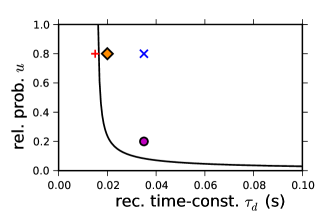
Figure 1: Phase diagram of a system with depressive couplings. The asynchronous stationary state is stable underneath the curve. The solid line correspond to the parameter regime where the purely imagery eigenvalues give rise to Hopf bifurcation of asynchronous irregular state. The marked symbols are the parameters in the phase space that we adopt to numerically evolve the system [Supplimantymatrialat]supp in Fig.2. Parameters: $\mu_{ext}$=0.95, $\sigma$=0.0228, ${g_{\mathrm{s}}}$=0.00245, $\tau_{m}$=0.020 and $\tau_{s2}$=0.001, $x_{\mathrm{thr}}$=1 and $V_{r}$=0.

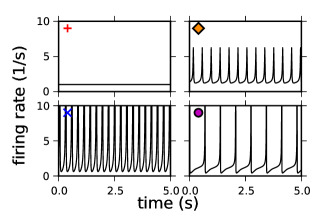
Figure 2: The numerical simulation of the full system with depressive couplings using population density treatment [Supplimantymatrialat]supp. Each subplot illustrates the population firing rate of the system with the parameters are marked with corresponding symbol in Fig.1.

In the present letter, we derived self-consistent description of the inter-event distribution of non-linear pulse coupled oscillators with interactions. We additionally characterized the asynchronous state and its stability. For static interactions, this result coincides with the result from the classical Fokker-Planck approach. However, as we showed our approach is easily extended to incorporate the effect of dynamical coupling. Using this, we investigated how networks with interaction through couplings with short-term depression undergoes a Hopf bifurcation to a state with collective synchronization, so-called population spikes. The method also allows for a efficient way to simulate the dynamics of systems in their thermodynamic limits [Supplimantymatrialat]supp. We showed in this limit the system may exhibit a super-critical Hopf bifurcation. Up to now, the collective effect of activity dependent modulation of interaction in a network has only been analyzed in models without non-linear contributions of the inter-event density cortes_short-term_2013 ; tsodyks_neural_1998 . In such networks interesting phenomena such a as Shilnikov chaos has been observed when positive feedback (e.g. facilitation) are added cortes_short-term_2013 . It is straightforward to extend our approach to study those cases where the network of oscillators with self-consistent inter-event density (e.g. spiking neurons) are also considered. The method presented in here relies on our ability to calculate $\hat{\rho}$, the solution of the unrestricted of Fokker-Planck equation. Once this is achieved imposing the necessary boundary conditions is easy using the presented method. Thus we believe that our approach will have a wide range of applications.

Acknowledgment. FF was funded by GIF-I-1224-396.13/2012. CvV was supported by ANR-BALWM grant.

References

• (1) Y. Kuramoto, Chemical oscillations, waves, and turbulence (Courier Dover Publications, 2003)
• (2) A. T. Winfree, The Geometry of Biological Time (Springer Science & Business Media, 2001)
• (3) H. Risken and T. Frank, The Fokker-Planck Equation: Methods of Solutions and Applications, 2nd ed. (Springer, 1996)
• (4) E. Schrödinger, Physikalische Zeitschrift 16, 289–295 (1915)
• (5) S. Chandrasekhar, The Astrophysical Journal 97, 263 (Mar. 1943)
• (6) M. C. Wang and G. E. Uhlenbeck, Reviews of Modern Physics 17, 323–342 (1945)
• (7) L. F. Abbott and C. van Vreeswijk, Physical Review E 48, 1483 (1993)
• (8) N. Brunel and V. Hakim, Chaos: An Interdisciplinary Journal of Nonlinear Science 18, 015113 (2008)
• (9) B. N. Kholodenko, Nature Reviews Molecular Cell Biology 7, 165 (Mar. 2006), 00731
• (10) S. Grossberg, Journal of Theoretical Biology 22, 325 (Feb. 1969)
• (11) M. Tsodyks, K. Pawelzik, and H. Markram, Neural Computation 10, 821 (1998)
• (12)  http://link.aps.org/doi
• (13) H. C. Tuckwell, Introduction to Theoretical Neurobiology: Volume 2, Nonlinear and Stochastic Theories (Cambridge University Press, 2005)
• (14) J. M. Cortes, M. Desroches, S. Rodrigues, R. Veltz, M. A. Muñoz, and T. J. Sejnowski, Proceedings of the National Academy of Sciences 110, 16610 (Oct. 2013)