Near Optimal Subdivision Algorithms for Real Root Isolation

Abstract

The problem of isolating real roots of a square-free polynomial inside a given interval $I_{0}$ is a fundamental problem. Subdivision based algorithms are a standard approach to solve this problem. Given an interval $I$, such algorithms rely on two predicates: an exclusion predicate, which if true means $I$ has no roots, and an inclusion predicate, which if true, reports an isolated root in $I$. If neither predicate holds, then we subdivide the interval and proceed recursively, starting from $I_{0}$. Example algorithms are Sturm’s method (predicates based on Sturm sequences), the Descartes method (using Descartes’s rule of signs), and Eval (using interval-arithmetic). For the canonical problem of isolating all real roots of a degree $n$ polynomial with integer coefficients of bit-length $L$, the subdivision tree size of (almost all) these algorithms is bounded by $O(n(L+\log n))$. This is known to be optimal for subdivision based algorithms.

We describe a subroutine that improves the running time of any subdivision algorithm for real root isolation. The subroutine first detects clusters of roots using a result of Ostrowski, and then uses Newton iteration to converge to them. Near a cluster, we switch to subdivision, and proceed recursively. The subroutine has the advantage that it is independent of the predicates used to terminate the subdivision. This gives us an alternative and simpler approach to recent developments of Sagraloff (2012) and Sagraloff-Mehlhorn (2013), assuming exact arithmetic.

The subdivision tree size of our algorithm using predicates based on Descartes’s rule of signs is bounded by $O(n\log n)$, which is better by $O(n\log L)$ compared to known results. Our analysis differs in two key aspects. First, we use the general technique of continuous amortization from Burr-Krahmer-Yap (2009), and second, we use the geometry of clusters of roots instead of the Davenport-Mahler bound. The analysis naturally extends to other predicates.

1 Introduction

Given a polynomial $f\in{\mathbb{R}}[x]$ of degree $n$, the problem is to isolate the real roots of $f$ in an input interval $I_{0}$, i.e., compute disjoint intervals which contain exactly one real root of $f$, and together contain all roots of $f$ in $I_{0}\cap{\mathbb{R}}$. Subdivision based algorithms have been successful in addressing the problem. A general subdivision algorithm uses two predicates, given an interval $I$: the exclusion predicate $C_{0}(I)$, which if true means $I$ has no roots; the inclusion predicate, $C_{1}(I)$, which if true means $I$ has exactly one root. The algorithm outputs a root-partition ${\cal P}$ of $I_{0}$, i.e., a set of pairwise disjoint open intervals such that for each interval either $C_{0}$ or $C_{1}$ holds, and $I_{0}\setminus{\cal P}$ contains no roots of $f$. To compute isolating intervals for roots of $f$, check the sign of $f$ at the endpoints of the intervals in ${\cal P}$ (this works if $f$ is square-free). The following generic subdivision algorithm constructs a root-partition:

Isolate$(I_{0})$ Input: $f\in{\mathbb{R}}[x]$ and an interval $I_{0}\subseteq{\mathbb{R}}$. Output: A root-partition ${\cal P}$ of $f$ in $I_{0}$. 0. Preprocessing step. 1. Initialize a queue $Q$ with $I_{0}$, and ${\cal P}\leftarrow\emptyset$. 2. While $Q$ is not empty Remove an interval $I=(a,b)$ from $Q$. If $C_{0}(I)\vee C_{1}(I)$ then add $I$ to ${\cal P}$. else $\triangleleft\;\;$Subdivide $I$ Let $m\leftarrow(a+b)/2$. Push $(a,m)$ and $(m,b)$ into $Q$. 3. Output ${\cal P}$.

The algorithm is guaranteed to terminate for square-free polynomials; otherwise we get an infinite sequence of intervals converging to a root of multiplicity greater than one. Some standard choices of the predicates and the corresponding algorithms are:

1. Sturm sequences and Sturm’s method [Dav85],

2. Descartes’s rule of signs and the Descartes method [CA76],

3. Interval-arithmetic based approaches and Eval [BKY09].

The complexity of these algorithms is well understood for the benchmark problem of isolating all real roots of a square-free integer polynomial with coefficients of bit-length $L$. One measure of complexity is the size of the subdivision tree constructed by the algorithm. For the first two algorithms a bound of $O(n(L+\log n))$ was shown in [Dav85] and [ESY06], respectively. For Eval a weaker bound of $O(n(L+n))$ was established in [SY12]. It is also known [ESY06] that the bound $O(n(L+\log n))$ is essentially tight for any algorithm doing uniform subdivision, i.e., reduces the width at every step by some constant (in our case by half).

Uniform subdivision cannot improve on the bound mentioned above because it only gives linear convergence to a “root cluster”, i.e., roots which are relatively closer to each other than to any other root. But it is known that from points sufficiently far away from the cluster, Newton iteration (more precisely, its variants for multiple roots) converges quadratically to the cluster. This has been an underlying idea in improving the linear convergence of subdivision algorithms for root isolation [Pan00, Sag12, SM13], and has also been combined with homotopy based approaches [Yak00, ST09].

We follow the same idea with some key differences. Given $C_{0}$ and $C_{1}$, our algorithm can be described as follows (we only give the inner loop, see Section 3 for complete details):

Newton-Isol$(I_{0})$ … If $C_{0}(I)\vee C_{1}(I)$ then add $I$ to ${\cal P}$. else if a cluster ${\cal C}$ of roots is detected in $I$ then Apply Newton iteration to approximate ${\cal C}$ while quadratic convergence holds. Estimate an interval $J$ containing ${\cal C}$. Push $J$ into $Q$. else  $\triangleleft\;\;$Subdivide $I$ …

For detecting root clusters, we use a result of Ostrowski based on Newton diagram of a polynomial [Ost40]; other choices are based on a generalization of Smale’s $\alpha$-theory (see [GLSY05] and the references therein); the details can be found in Section 2. These tools and approaches have been used earlier [Pan00], however, our approach has the following differences:

1. The tools used to detect and estimate the size of a cluster are independent of the particular choice of the exclusion-inclusion predicates (cf. [Sag12]). This way we obtain a general approach to improve any subdivision algorithm.

2. Another difference is the method that is combined with bisection to improve convergence. In [Sag12] Abbott’s QIR method is combined with the Schröder operator [GLSY05], whereas we apply standard Newton iteration to a suitable derivative of $f$. The former combination is a backtracking approach to get quadratic convergence; the latter gives quadratic convergence right away (but perhaps increasing subdivisions). This has the advantage of separating the Newton iteration steps from the subdivision tree, which is reflected in the bounds on the subdivision tree size for the two approaches: for the former we have $O(n\log(nL))$, and for the latter we have $O(n\log n)$. The number of quadratically converging steps remains the same in both cases.

3. Our approach can be modified to isolate complex roots; replace binary subdivision with a quad-tree subdivision, and choose appropriate predicates (e.g., Ostrowski’s result mentioned above, or Pellet’s test). This avoids Graeffe iteration (cf. [Pan00]), and yet the modified algorithm can be shown to attain a near optimal bound on subdivision tree size.

In this paper, we focus on bounding the size of subdivision tree of Newton-Isol. For this purpose, we use the general framework of continuous amortization [BKY09, Bur13]. The key idea here is to bound the tree size by $\int_{I_{0}}G(x)dx$, where $G$ is a suitable “charging” function corresponding to the predicates used in the algorithm (e.g., see [Bur13]). Our key contributions are the following:

1. We derive a near optimal bound of $O(n\log n)$ on the size of the subdivision tree of Newton-Isol when $C_{0}$, $C_{1}$ are based on Descartes’s rule of signs (see Theorem 10). This is the first application of the continuous amortization framework to a non-uniform subdivision algorithm.

2. We show that if the distance of the cluster center to the nearest root outside the cluster exceeds roughly $n^{3}$ times the diameter of the cluster, then Ostrowski’s criterion for cluster detection works, and we obtain quadratic convergence to the cluster center (see Lemma 6).

3. Our analysis crucially uses the cluster tree of the polynomial (see Proposition 1). We derive an integral bound on the size of the subdivision tree (see Theorem 9). The usual approach to upper bound this integral is to break it over the (real) Voronoi regions of the roots [Bur13]. We instead break the integral over the Voronoi regions corresponding to the clusters in an inductive manner based on the cluster tree. The integral over the portion of the region outside the cluster is bounded using known techniques. However, for the portion inside the cluster, we devise an amortized bound on the integral (see Lemma 12), which is of independent interest, and is analogous to the improvement given by Davenport-Mahler bound over repeated applications of the root separation bound. It is this result that underlies the $O(n\log n)$ bound. A simple argument extends these bounds to Sturm’s method and the Eval algorithm. The details are in Section 4.

2 Notation and Basic Results

Let $f\in{\mathbb{R}}[x]$ be a square-free polynomial of degree $n\geq 2$ and $Z(f)\subset{\mathbb{C}}$ be its set of roots. Given a finite pointset $S\subseteq{\mathbb{R}}^{2}$, let $D_{S}$ be the disc $D(m_{S},r_{S})$ such that $m_{S}$ is the centroid of the points in $S$, and $r_{S}$ is the least radius such that all the points in $S$ are contained in $D(m_{S},r_{S})$. Given a $\lambda\in{\mathbb{R}}_{>0}$, define $\lambda D_{S}{\color[rgb]{1,0,0}\mathrel{\,:=\,}}D(m_{S},\lambda r_{S})$. We borrow the following definition from [SSY13]: A subset ${\cal C}\subseteq Z(f)$ of size at least two is called a (root) cluster if the only roots in $3D_{\cal C}$ are from ${\cal C}$. We treat individual roots as (trivial) clusters. In this paper, the non-real roots in ${\cal C}$ come in conjugate pairs. Therefore, the center of $D_{\cal C}$ will always be in ${\mathbb{R}}$. Define $R_{\cal C}$ as the distance from $m_{\cal C}$ to the nearest point in the set $Z(f)\setminus{\cal C}$. From the definition it follows that $Z(f)$ trivially forms a cluster and $R_{Z(f)}=\infty$. Given an interval $I$, let $m(I)$ denote its midpoint and $w(I)$ its width. We will often use the shorthand $I=[m(I)\pm w(I)/2]$, and for $\lambda>0$, $\lambda I{\color[rgb]{1,0,0}\mathrel{\,:=\,}}[m(I)\pm\lambda w(I)/2]$. An interval $I$ contains a cluster ${\cal C}$ if ${\cal C}\subseteq D(m(I),w(I)/2)$.

We use the following convenient notation in the subsequent definitions: for $x,y\in{\mathbb{R}}$, ‘$x\gg y$’ if there is a constant $c\geq 1$ such that $x\geq cy$; similarly define $x\ll y$.

A strongly-separated cluster (ssc) is a cluster ${\cal C}$ for which $R_{\cal C}/r_{\cal C}\gg n^{3}$; the exact constant can be found in Corollary 7. For a ssc ${\cal C}$, define the following three quantities:

1. The interval $I_{\cal C}{\color[rgb]{1,0,0}\mathrel{\,:=\,}}[m_{\cal C}\pm c\cdot kr_{\cal C}]$, for some constant $c\geq 1$.

2. The interval ${\cal I}_{\cal C}{\color[rgb]{1,0,0}\mathrel{\,:=\,}}\left\{x:|x-m_{\cal C}|\ll R_{\cal C}/n^{2}\right\}$.

3. The annulus ${\cal A}_{\cal C}{\color[rgb]{1,0,0}\mathrel{\,:=\,}}{\cal I}_{\cal C}\setminus I_{\cal C}=\left\{z\in{\mathbb{C}}:|{\cal C}|r_{\cal C}\ll|z-m_{\cal C}|\ll R_{\cal C}/n^{2}\right\}$.

The exact constants in these definitions are given in Lemma 6. See Figure 1 for an illustration of these concepts. If ${\cal C}$ is not a ssc, then we define $I_{\cal C}{\color[rgb]{1,0,0}\mathrel{\,:=\,}}[m_{\cal C}\pm r_{\cal C}]$ and ${\cal I}_{\cal C}{\color[rgb]{1,0,0}\mathrel{\,:=\,}}2I_{\cal C}$. Note that for all clusters ${\cal C}$, $I_{\cal C}\subseteq{\cal I}_{\cal C}$. We will need the following result later in our analysis [SSY13, Lemma 2.1]:

Proposition 1.

Given a root cluster ${\cal C}$ of $f$. There is a unique unordered tree $T_{\cal C}$ rooted at ${\cal C}$ whose set of nodes are the clusters contained in ${\cal C}$, and the parent-child relation is subset inclusion. Let $T_{f}$ be the tree where the parent is the cluster $Z(f)$ of all roots.

The result originally is stated for root clusters of $f\in{\mathbb{C}}[x]$. However, for $f\in{\mathbb{R}}[x]$ the clusters come in conjugate pairs, and by taking the union of such pairs the result still holds. The tree $T_{\cal C}$ is called the cluster tree of ${\cal C}$. The leaves of this tree are the roots in ${\cal C}$.

Figure 1: Geometry of a ssc ${\cal C}$. We focus on the the relative geometry, overlooking the exact constants involved in the definition of the intervals.

2.1 Cluster Detection and Approximation

The literature on detection and approximation of root clusters is vast (see [GLSY05] and the references therein). One approach is based on Pellet’s test: if for a complex polynomial $f(x)=\sum_{i=0}^{n}a_{i}x^{i}$ there is an $r>0$ such that $|a_{k}|r^{k}>\sum_{i\neq k}|a_{i}|r^{i}$ then the disc $D(0,r)$ contains exactly $k$ roots of $f$. A point $z\in{\mathbb{C}}$ is said to satisfy Pellet’s test, if there is a $k$ and $r$ for which the test holds with the coefficients of $f(x+z)$. Results in [Yak00, GLSY05] generalize Smale’s $\alpha$-theory and relate it to Pellet’s test; an alternative derivation based on tropical algebra is given in [Sha11]. We instead use a result by Ostrowski [Ost40].

We need the following definitions. Let $f(x)=\sum_{i=0}^{n}a_{i}x^{i}$, where $a_{i}\in{\mathbb{C}}$. With each index $i$, $a_{i}\neq 0$, associate the point $P_{i}{\color[rgb]{1,0,0}\mathrel{\,:=\,}}(i,-\log|a_{i}|)\in{\mathbb{R}}^{2}$. The lower-hull of the convex-hull of these points is called the Newton diagram of $f$. Given an index $k\in\left\{0,\ldots,n\right\}$, let $y_{k}$ be the point such that $(k,y_{k})$ is on the diagram. Define $\rho_{k}{\color[rgb]{1,0,0}\mathrel{\,:=\,}}e^{y_{k}-y_{k-1}}$, for $1\leq k\leq n$, $\rho_{n+1}{\color[rgb]{1,0,0}\mathrel{\,:=\,}}\infty$, and the $k$th deviation $\Delta_{k}{\color[rgb]{1,0,0}\mathrel{\,:=\,}}\rho_{k+1}/\rho_{k}$, for $0<k<n$.

Let $\alpha_{1},\ldots,\alpha_{n}\in{\mathbb{C}}$ be the roots of $f$ ordered such that $|\alpha_{1}|\leq|\alpha_{2}|\leq\cdots\leq|\alpha_{n}|$. Ostrowski showed the following fundamental relation between the absolute values of the roots and $\rho_{k}$’s [Ost40, p. 143]:

$$\frac{1}{2k}<\frac{|\alpha_{k}|}{\rho_{k}}<2(n-k+1).$$ (1)

Given $z\in{\mathbb{C}}$, we will be interested in the Newton diagram of $f(x+z)$. If $f_{j}(z){\color[rgb]{1,0,0}\mathrel{\,:=\,}}f^{(j)}(z)/j!$, then from a result of Ostrowski [Ost40, p. 128] we get:

$$\rho_{k}(z)=\max_{j<k}\left\lvert\frac{f_{j}(z)}{f_{k}(z)}\right\rvert^{\frac{1}{(k-j)}},\text{ and }\rho_{k+1}(z)=\min_{j>k}\left\lvert\frac{f_{k}(z)}{f_{j}(z)}\right\rvert^{\frac{1}{(j-k)}}.$$ (2)

The RHS is defined for any $k$ such that $f_{k}(z)\neq 0$; however, we are only interested in those $k$ for which $P_{k}$ is on the diagram. The $k$th deviation $\Delta_{k}(z){\color[rgb]{1,0,0}\mathrel{\,:=\,}}\rho_{k+1}(z)/\rho_{k}(z)$. We have the following result for detecting clusters:

Lemma 2.

If $\Delta_{k}(z)\geq 27$, for some index $0<k<n$, then there are exactly $k$ roots in $D(z,3\rho_{k}(z))$ and $D(z,\rho_{k+1}(z)/3)$. Moreover, as $\rho_{k+1}(z)/3\geq 9\rho_{k}(z)$, these roots form a cluster.

The proof shows that the inequality $\Delta_{k}(z)\geq 27$ implies that Pellet’s test holds for $D(z,r)$, $3\rho_{k}(z)\leq r\leq D(z,\rho_{k+1}(z)/3)$ (see [GLSY05, Thm. 1.5]). Since the $P_{i}$’s are sorted by x-coordinate, all the $\rho_{k}$’s can be computed in $O(n)$ steps using, e.g., Graham’s scan for convex hull computation.

Once we have detected a cluster ${\cal C}$ near $z$, we want a good approximation to $m_{\cal C}$. A standard way is to do the iteration $z_{i+1}=z_{i}-kf(z_{i})/f^{\prime}(z_{i})$, starting from $z$, but this may not be numerically desirable, as both $f$ and $f^{\prime}$ are small near ${\cal C}$. Another option is to use the standard Newton iteration applied to $f^{(k-1)}$. We show that if $\Delta_{k}(z)\geq 27$, then $z$ is an approximate zero, in the sense of Smale et al. [BCSS98, p. 160, Thm. 2], to the root of $f^{(k-1)}$ in $D(z,\frac{3\rho_{k}(z)}{2k})$. Subsequently we show that if $\Delta_{k}(z)\geq c_{0}$, for some constant $c_{0}\geq 27$, then for all $z^{\prime}$ in this disc $\Delta_{k}(z^{\prime})\geq 27$, and hence there is a cluster of $k$ roots in $D(z^{\prime},3\rho_{k}(z^{\prime}))$. Moreover, the cluster is exactly ${\cal C}$. These results are summarized in the following:

Lemma 3.

Let $z\in{\mathbb{C}}$ be such that $\Delta_{k}(z)\geq c_{0}$, for some $k\geq 2$, ${\cal C}$ be the cluster in $D(z,3\rho_{k}(z))$, and $D^{\prime}{\color[rgb]{1,0,0}\mathrel{\,:=\,}}D(z,\frac{3\rho_{k}(z)}{2k})$. Then the following hold:

1. $z$ is an approximate zero to the root $z^{*}$ of $f^{(k-1)}$ in $D^{\prime}$ and the Newton iterates starting from $z$ are in $D^{\prime}$.

2. For all $z^{\prime}\in D^{\prime}$, $\Delta_{k}(z^{\prime})\geq 27$, and ${\cal C}$ is the cluster in $D(z^{\prime},3\rho_{k}(z^{\prime}))$.

3. If $z,w$ are such that $\Delta_{k}(z),\Delta_{k}(w)\geq 27$ and $D(z,3\rho_{k}(z))$, $D(w,3\rho_{k}(w))$ intersect then the discs have the same cluster.

The proof is given in the appendix. We choose $c_{0}{\color[rgb]{1,0,0}\mathrel{\,:=\,}}27\times 6e^{6}$. Given $z\in{\mathbb{C}}$, a value of $k$ satisfying the condition $\Delta_{k}(z)\geq c_{0}$ is called an admissible value for $z$, with the corresponding inclusion disc $D(z,3\rho_{k}(z))$. Note that there can be more than one admissible value for a point $z$ corresponding to clusters of different sizes.

3 The Algorithm

Let $C_{0}$ and $C_{1}$ be some exclusion and inclusion predicate respectively. The following algorithm takes as input $f$ and an interval $I_{0}$ and outputs a root partition of $I_{0}$.

Newton-Isol$(f,I_{0})$ 1 Initialize ${\cal P}\leftarrow\emptyset$, $\Phi\leftarrow\emptyset$; let $Q$ be an empty queue. 1.a. If this is a recursive call then subdivide $I_{0}$ and push the two halves into $Q$; else $Q\leftarrow\left\{I_{0}\right\}$. 2. While $Q$ is not empty do Remove an interval $I$ from $Q$. 2.a. If $C_{0}(I)\vee C_{1}(I)$ then add $I$ to ${\cal P}$. else if Newton-Incl-Exc($I$) is successful then Let $(J,k)$ be the pair returned. 2.b. If $\forall J^{\prime}\in\Phi$, $J\cap J^{\prime}=\emptyset$ and $J\cap I_{0}\neq\emptyset$ then 2.c. $\forall$ $I^{\prime}\in Q$, $I^{\prime}\leftarrow I^{\prime}\setminus D(m(J),\frac{\rho_{k+1}(m(J))}{3})$. 2.d. Add $J\cap I_{0}$ to $\Phi$. else subdivide $I$ and push the two halves into $Q$. 3. Return ${\cal P}\cup_{J\in\Phi}\texttt{Newton-Isol}(f,J)$.

The input to Newton-Incl-Exc is an interval $I=(a,b)$. If the predicate is successful then it returns an interval $J$ containing a cluster such that $w(J)<w(I)/2$, and an admissible value $k$ for $m(J)$; otherwise it returns failure.

Newton-Incl-Exc $(f,I)$ 1. Let $m{\color[rgb]{1,0,0}\mathrel{\,:=\,}}(a+b)/2$. 2. For $p\in\left\{a,m,b\right\}$, let $k_{p}\geq 2$ be the smallest admissible value $k$ for $p$ such that $I\subseteq D\left({p,\frac{\rho_{k+1}(p)}{3}}\right)$. 3. If the three admissible values are equal and the three inclusion discs are contained in $D\left({m,\frac{\rho_{k_{m}+1}(m)}{3}}\right)$ then: 3.a. $z_{0}{\color[rgb]{1,0,0}\mathrel{\,:=\,}}m$, $k{\color[rgb]{1,0,0}\mathrel{\,:=\,}}k_{m}$, $g{\color[rgb]{1,0,0}\mathrel{\,:=\,}}f^{(k-1)}$, $i{\color[rgb]{1,0,0}\mathrel{\,:=\,}}0$. 4. While $\rho_{k}(z_{i})\leq 2^{5-2^{i}}\rho_{k}(z_{0})$ $z_{i+1}{\color[rgb]{1,0,0}\mathrel{\,:=\,}}z_{i}-g(z_{i})/g^{\prime}(z_{i})$; $i{\color[rgb]{1,0,0}\mathrel{\,:=\,}}i+1$. $J{\color[rgb]{1,0,0}\mathrel{\,:=\,}}[z_{i-1}\pm 3\rho_{k}(z_{i-1})]$ 5. If $w(J)\geq w(I)/2$ then return failure 6. else return $(J,k)$. 7. Return failure.

We first explain some steps in the predicate above:

1. Step 2. A point $p$ in $I$ can have more than one admissible value associated with it. The right admissible value is governed by $w(I)$, since we should only consider those clusters ${\cal C}$ for which $r_{\cal C}\ll w(I)\ll R_{\cal C}$.

2. Step 3. As $D(m,\rho_{k_{m}+1}(m)/3)$ contains all the three inclusion discs, they all contain the same cluster ${\cal C}$. Otherwise, it is possible that the three inclusion discs contain different clusters but of the same size.

3. Step 4. This ensures that as $z_{i}$ converges to the root of $f^{(k-1)}$, the distance to ${\cal C}$ decreases quadratically; this fails when we are near ${\cal C}$, or the root of $f^{(k-1)}$ is not near ${\cal C}$.

4. Step 5. Required to ensure linear convergence to ${\cal C}$.

5. Step 6. The interval $J$ contains the cluster ${\cal C}$. Moreover, as $I\subseteq D(m,\rho_{k+1}(m)/3)$, we know that if the roots in $I$ are a subset of ${\cal C}$, and hence are inside $J$. By now $w(J)<w(I)/2$, therefore, it suffices to return $J$.

We now comment on some steps in Newton-Isol:

1. Step 1.a. Ensures that a successful call to Newton-Incl-Exc is followed by a subdivision step. Thus the recursion tree is a binary tree. The predicate can still be successful on an interval $J$ returned by an earlier successful call. But the convergence in this case would only be linear, and so we prefer subdivision, though in practice one can go ahead with the linear convergence.

2. Step 2.b. Checks if ${\cal C}$ has not been found before (see Lemma 3(iii)), and that $J$ is inside $I_{0}$; if either of this test fails, then $I$ contains no roots and can be excluded.

3. Step 2.c. As the only cluster in $D(m(J),\frac{\rho_{k+1}(m(J))}{3})$ is ${\cal C}$, we can remove this disc from the intervals in $Q$. It is this exclusion step that significantly contributes to the improvement of the subdivision algorithm.

4. Step 2.d. This step adds the interval $J\cap I_{0}$ containing the newly discovered cluster ${\cal C}$ to the set $\Phi$.

There are only two loops in the algorithm: first, the while-loop in step 2 of the algorithm, and second, the Newton iteration in step 4 of Newton-Incl-Exc. The argument for the termination of the first loop is the same as for Isolate. The termination of the second loop is guaranteed, because if $z_{i}$’s are such that $\rho_{k}(z_{i})$ keeps on decreasing, then in the limit $\rho_{k}$’s converge to zero; but the disc $D(z_{i},3\rho_{k}(z_{i}))$ contains exactly $k$ roots; since, in the limit $z_{i}$’s tend to a root $z^{*}$ of $f^{(k-1)}$, this implies that $z^{*}$ is a $k$-fold root of $f$, which is a contradiction as $f$ is square-free.

The following is a proof of correctness of the algorithm.

Theorem 4.

Given a polynomial $f$ and an interval $I_{0}$, Newton-Isol$(f,I_{0})$ outputs a root partition ${\cal P}$ of $I_{0}$.

Proof. We need to show the following claims:
1. $I_{0}\setminus{\cal P}$ contains no real roots of $f$.
2. ${\cal P}$ contains (interior) pairwise disjoint intervals.
3. For all $I\in{\cal P}$, $C_{0}$ or $C_{1}$ holds (follows from step 2.a.).

Lemma 3 gives us the correctness of Newton-Incl-Exc$(I)$, i.e., if the test is successful then it returns an interval $J$ such that any roots in $I$ are contained in $J$. We only argue for the first claim. For every interval $J$ returned by a successful call of the predicate, define

$$A_{J}{\color[rgb]{1,0,0}\mathrel{\,:=\,}}D\left({m(J),{\rho_{k+1}(m(J))}/{3}}\right)\setminus D(m(J),w(J)/2),$$ (3)

i.e., the annulus around $J$ that does not contain any roots. We exclude intervals if step (2.b) fails for the interval $J$, or a portion of an interval is removed in step (2.c.). In the former case, either the cluster contained in $J$ was already detected, or it is outside $I_{0}$. In the latter case, we do not loose any roots since $A_{J}$ has no roots. So $I_{0}\setminus{\cal P}$ contains no roots.   Q.E.D.

4 Complexity Analysis

The main result is that Newton-Incl-Exc will be successful near a ssc ${\cal C}$. Let $c_{0}>20$ be the constant in Lemma 3, and ${\cal C}$ a ssc throughout this section. Our first claim is that $|{\cal C}|$ is an admissible value for all points in ${\cal I}_{\cal C}$.

Lemma 5.

If $|z-m_{\cal C}|\leq R_{\cal C}/(8c_{0}n^{2})$ then $\Delta_{k}(z)\geq c_{0}$.

Proof. Let $\alpha_{1},\ldots,\alpha_{k}\in{\cal C}$ and $\alpha_{k+1},\ldots,\alpha_{n}\in Z(f)\setminus{\cal C}$. Moreover, assume that they are ordered in increasing distance from $z$. From (1), we know that $2k|z-\alpha_{k+1}|>\rho_{k+1}(z)>|z-\alpha_{k+1}|/(2(n-k+1))$. Moreover, $|z-\alpha_{k+1}|>R_{\cal C}-|z-m_{\cal C}|\geq R_{\cal C}/2$; similarly, $|z-\alpha_{k+1}|<3R_{\cal C}/2$. Therefore,

$$\frac{R_{\cal C}}{4n}\leq\rho_{k+1}(z)\leq 3|{\cal C}|R_{\cal C}.$$ (4)

From (1), we again have $\rho_{k}(z)<2k|z-\alpha_{k}|$. But $|z-\alpha_{k}|\leq|z-m_{\cal C}|+r_{\cal C}$, which gives us

$$\rho_{k}(z)\leq 2k(|z-m_{\cal C}|+r_{\cal C}).$$ (5)

Since $|z-m_{\cal C}|,r_{\cal C}\leq R_{\cal C}/(8c_{0}n^{2})$, we get $\rho_{k}(z)\leq kR_{\cal C}/(2c_{0}n^{2})$. Combining this with (4), and the observation that $(n-k)k\leq n^{2}/4$, we obtain that $\Delta_{k}\geq 2c_{0}n^{2}/(8(n-k)k)\geq c_{0}$.   Q.E.D.

Recall the definition of the intervals $I_{\cal C}$, ${\cal I}_{\cal C}$ and the annulus ${\cal A}_{\cal C}$ from Section 2, and $A_{J}$ from (3).

Lemma 6.

If an interval $I$ is such that

$$I\subseteq{\cal I}_{\cal C}=[m_{\cal C}\pm R_{\cal C}/(8c_{0}n^{2})]\text{ and }w(I)>72|{\cal C}|r_{\cal C}$$

then the pair $(J,k)$ returned by Newton-Incl-Exc$(I)$ is such that $k=|{\cal C}|$, $J\subseteq I_{\cal C}=[m_{\cal C}\pm 20kr_{\cal C}]$, and $A_{J}\supseteq{\cal A}_{\cal C}$.

Proof. We show that the conditions on $I$ above imply that Newton-Incl-Exc$(I)$ reaches step 6 of Newton-Incl-Exc (all the steps below refer to the steps in the predicate). This requires showing the following: (i) all the conditions in step 3 are met; (ii) Newton-iteration in step 4 converges quadratically terminating with an interval $J$ with $w(J)<w(I)/2$, and (iii) $J\subseteq I_{\cal C}$. The following claims provide the proof. Let $I=[a,b]$ and $m=m(I)$.

1. Claim 1: For all $p\in\left\{a,m,b\right\}$, $k_{p}=|{\cal C}|$. Recall from Step 2 that $k_{p}$ is defined as the smallest admissible value $k$ for which $I\subset D(p,\rho_{k+1}(p)/3)$. From Lemma 5, we have $k_{p}\leq|{\cal C}|$. Since the roots in $I$ can only come from ${\cal C}$, any smaller admissible value corresponds to a subcluster ${\cal C}^{\prime}$ of ${\cal C}$, which implies $R_{{\cal C}^{\prime}}\leq r_{\cal C}$. From (4) we know that $\rho_{|{\cal C}^{\prime}|+1}(p)\leq 3(|{\cal C}^{\prime}|+1)R_{{\cal C}^{\prime}}\leq 3|{\cal C}|r_{\cal C}$. Since $w(I)\geq 72|{\cal C}|r_{\cal C}$, clearly $I\not\subseteq D(p,\rho_{|{\cal C}^{\prime}|+1}(p)/3)$ for any subcluster ${\cal C}^{\prime}\subset{\cal C}$. Thus $k_{p}\geq|{\cal C}|$.
   

2. Claim 2: For all $p\in I$, $I\subseteq D(p,\rho_{k+1}(p)/3)$. This will follow from the more general claim that

   $$D_{1}{\color[rgb]{1,0,0}\mathrel{\,:=\,}}D(m_{\cal C},R_{\cal C}/(8c_{0}n^{2}))\subseteq D(z,\rho_{|{\cal C}|+1}(z)/3)\mathop{\mbox{\rm=:}}D_{2},$$

   for all $z\in D_{1}$; since $a,m,n\in I\subseteq D_{1}$, the claim holds. But for any $z\in D_{1}$, we know from (4) that $\frac{\rho_{|{\cal C}|+1}(z)}{3}\geq\frac{R_{\cal C}}{12n}$ which is greater than $\frac{R_{\cal C}}{4c_{0}n^{2}}$, the diameter of $D_{1}$, for $c_{0}\geq 3$.

3. Claim 3: For all $z,w\in D_{1}$, the inclusion disc $D(z,3\rho_{k}(z))\subseteq D(w,\frac{\rho_{k+1}(w)}{3})$. This follows if

   $$|z-w|+3\rho_{k}(z)\leq\frac{\rho_{k+1}(w)}{3}.$$ (6)

   But $|z-w|,r_{\cal C}\leq R_{\cal C}/(8c_{0}n^{2})$, which along with (5) implies that $3\rho_{k}(z)\leq 6kR_{\cal C}/(4c_{0}n^{2})$. Therefore, LHS of (6) is smaller than $13kR_{\cal C}/(8c_{0}n^{2})$, which is smaller than $R_{\cal C}/(12n)$ for $c_{0}\geq 20$, but from (4) we know that the latter is smaller than the RHS of (6).
   

4. Claim 4: Let $z_{i}$ be the sequence of iterates computed in the while-loop in Step 4. If $z_{i}\in D(m_{\cal C},\frac{R_{\cal C}}{8c_{0}n^{2}})\setminus D(m_{\cal C},2r_{\cal C})$, then $\rho_{k}(z_{i})<2^{5-2^{i}}\rho_{k}(z_{0})$. Since $z_{i}\not\in D(m_{\cal C},2r_{\cal C})$, $r_{\cal C}\leq|z_{i}-m_{\cal C}|$, and hence from (5) we obtain $\rho_{k}(z_{i})\leq 4k|z_{i}-m_{\cal C}|$. From [Paw99, Thm. 2.2] we know that there is a unique root $z^{*}$ of $f^{(k-1)}$ in $D(m_{\cal C},r_{\cal C})$. Therefore, $|z_{i}-m_{\cal C}|\leq|z_{i}-z^{*}|+r_{\cal C}$. But as $z_{i}\not\in D(m_{\cal C},2r_{\cal C})$ and $z^{*}\in D(m_{\cal C},r_{\cal C})$, we have $r_{\cal C}\leq|z_{i}-z^{*}|$, and hence $|z_{i}-m_{\cal C}|\leq 2|z_{i}-z^{*}|$. Thus, $\rho_{k}(z_{i})\leq 8k|z_{i}-z^{*}|$. As $z_{0}$ is an approximate zero to $z^{*}$ (see Lemma 3(i)), we know $|z_{i}-z^{*}|\leq 2^{1-2^{i}}|z_{0}-z^{*}|$, which implies that $\rho_{k}(z_{i})\leq 2^{4-2^{i}}k|z_{0}-z^{*}|$. Furthermore, from Lemma 3(i) we know $k|z_{0}-z^{*}|<2\rho_{k}(z_{0})$. Hence $\rho_{k}(z_{i})<2^{5-2^{i}}\rho_{k}(z_{0})$.
   

5. Claim 5: The interval $J\subseteq I_{\cal C}$ and $w(J)<w(I)/2$. The previous claim shows that if $z_{i}\not\in D(m_{\cal C},2r_{\cal C})$, then we will obtain quadratically decreasing values of $\rho_{k}(z_{i})$. Thus when the iteration stops $z_{i}\in D(m_{\cal C},2r_{\cal C})$, and it follows from (5) that $\rho_{k}(z_{i})\leq 6kr_{\cal C}$. Hence the interval $J=z_{i}\pm 3\rho_{k}(z_{i})$ is contained in $I_{\cal C}$, for $k\geq 2$. Moreover, $w(J)\leq 36kr_{\cal C}<w(I)/2$, and hence the condition in Step 5 fails and we return $J$. The claim on the annulus follows from (4).

Q.E.D.

The following result translates the result above in terms of the subdivision tree:

Corollary 7.

Let ${\cal C}$ be a ssc such that ${\cal I}_{\cal C}\subseteq I_{0}$. If $I$ is the first interval such that Newton-Incl-Exc$(I)$ is successful and the interval returned contains ${\cal C}$, then ${\cal I}_{\cal C}\subseteq I^{\prime}\cup I^{\prime\prime}$, where $I^{\prime}$ is the parent-interval of $I$ and $I^{\prime\prime}$ is one of $I^{\prime}$’s neighbors.

Proof. In the worst case, ${\cal C}$ will be detected the first time in the subdivision tree an interval $I\subseteq{\cal I}_{\cal C}$. For such an $I$, we show $w(I)\gg kr_{\cal C}$. Since $I$ is the first interval to fall in ${\cal I}_{\cal C}$, both $I^{\prime}$ and $I^{\prime\prime}$ have endpoints outside ${\cal I}_{\cal C}$, thus ${\cal I}_{\cal C}\subseteq I^{\prime}\cup I^{\prime\prime}$. So $2w(I)\geq R_{\cal C}/(16c_{0}n^{2})>72kr_{\cal C}$, as ${\cal C}$ is ssc. The claim clearly holds if ${\cal C}$ is detected at an ancestor of $I$.   Q.E.D.

Remark: The proof above gives us the explicit constant in the definition of ssc, namely, we require $R_{\cal C}/r_{\cal C}>16c_{0}\times 72n^{3}$. A careful working out of the proofs shows that the weaker inequality $R_{\cal C}/r_{\cal C}>4c_{0}\times 72(n-|{\cal C}|)|{\cal C}|^{2}$, (or even $50c_{0}n^{3}$) is sufficient.

Recall that the set of all roots $Z(f)$ is a cluster. As a consequence of Lemma 6, we assume that $I_{0}\subseteq nI_{Z(f)}$; otherwise Newton-Incl-Exc will be successful right away and the interval returned will satisfy the property.

4.1 An Integral Bound on the Subdivision Tree

Let ${\cal N}(I_{0})$ be the set of leaves in the subdivision tree of Newton-Isol$(f,I_{0})$. Step 1.a. of the algorithm ensures that the subdivision tree is a binary tree. Therefore, it suffices to bound $|{\cal N}(I_{0})|$. For this purpose, we use the general framework of continuous amortization developed in [BKY09] and generalized in [Bur13]. The idea is to bound $|{\cal N}(I_{0})|$ by an integral and then derive an upper bound on this integral. For this purpose we need the following notion: Given a choice of predicates $C_{0}$, $C_{1}$, a function $G:{\mathbb{R}}\to{\mathbb{R}}_{\geq 0}$ is called a stopping function corresponding to $C_{0}$ and $C_{1}$ if for every interval $I$, if there is an $x\in I$ such that $w(I)G(x)\leq 1$, then either $C_{0}(I)$ or $C_{1}(I)$ holds. Stopping functions, corresponding to different predicates, are provided in [Bur13]. The crucial property of $G(x)$ is the following:

Lemma 8.

If $C_{0}(I)$ and $C_{1}(I)$ fail for an interval $I$, then for all $J\subseteq I$, such that $2w(J)\geq w(I)$, $2\int_{J}G(x)dx\geq 1$.

Proof. From the definition of $G(x)$, we have for all $x\in I$, $G(x)w(I)\geq 1$. As $J\subseteq I$, $\forall x\in J$, $2G(x)w(J)\geq G(x)w(I)\geq 1$. Thus $2\int_{J}G(x)dx\geq 2w(J)\min_{x\in J}G(x)\geq 1$.   Q.E.D.

The main result of this section is the following:

Theorem 9.

$$|{\cal N}(I_{0})|\leq 4n+2\int_{I_{0}\setminus\cup_{\cal C}{\cal A}_{\cal C}}G(x)dx,$$

where the union is over all ssc ${\cal C}$ in $T_{f}$.

We bound ${\cal N}(I_{0})$ recursively. The leaves in ${\cal N}(I_{0})$ correspond to three types of intervals:

1. intervals in the root partition ${\cal P}$,

2. intervals that were discarded in step 2.c., and

3. intervals for which condition 2.b fails to hold (either cluster already found, or $J\cap I_{0}=\emptyset$).

We will bound each of these three types. We analyse what happens before the first set of recursive calls.

Let $\Phi$ be the set of intervals collected in Step 2.d. of the algorithm, $A_{J}$ be as defined in (3), and ${\cal I}_{J}{\color[rgb]{1,0,0}\mathrel{\,:=\,}}J\cup A_{J}$. From the construction of $\Phi$, we know that all intervals $J\in\Phi$ are contained in $I_{0}$ and each contains a unique cluster. For each $J\in\Phi$, let $L_{J}$ be the set of parent-intervals of intervals in $Q$ that intersect ${\cal I}_{J}$; the type (ii) intervals are children of intervals in $L_{J}$. Let $M_{J}$ be the set of intervals that do not intersect ${\cal I}_{J}$ and are of type (iii). See Figure 2 for an illustration of these types. Note that if $I\in L_{J}$ contains an endpoint of ${\cal I}_{J}$, then $I\setminus{\cal I}_{J}$ can be of type (i) or (iii); but there can be at most two such intervals for each $J$ on either side of ${\cal I}_{J}$. We abuse notation and use $L_{J}$ to represent a set as well as the union of the intervals in it; same for $M_{J}$.

Figure 2: The three types of intervals in ${\cal N}(I_{0})$. Intervals in $L_{J}$ are shown in green. The remaining intervals could be in $M_{J}$ or ${\cal P}$. The width of the red colored intervals can be much smaller than their parents. But there are at most two such intervals.

For an $I\in M_{J}$, both $C_{0}$ and $C_{1}$ failed. Therefore, from Lemma 8 we get $|M_{J}|\leq 2\sum_{I\in M_{J}}\int_{I}G(x)dx=2\int_{M_{J}}G(x)dx$. As the predicates $C_{0}$ and $C_{1}$ also fail for the intervals in $L_{J}$, we can similarly bound $|L_{J}|$. But this effectively amounts to doing subdivision on $J$. To avoid this we do the following: since the width of the intervals in $L_{J}$ is more than $w(J)$, we know that there are at most two neighboring intervals $I^{\prime}_{J}$ and $I^{\prime\prime}_{J}$ that contain $J$. We count them separately, and for the rest we use Lemma 8 to get $|L_{J}|\leq 2+2\int_{L_{J}\setminus(I^{\prime}_{J}\cup I^{\prime\prime}_{J})}G(x)dx$. For an interval $I\in{\cal P}$, we expect $2\int_{I}G(x)dx\geq 1$, as the predicates must have failed for the parent $I^{\prime}$ of $I$. However, Lemma 8 requires that $w(I^{\prime})\leq 2w(I)$. This can fail to happen near the boundary of ${\cal I}_{J}$, as noted earlier. But then there are at most two such intervals. Therefore, the number of intervals in ${\cal P}$ coming from the non-recursive calls is at most $2|\Phi|+2\int_{I_{0}\setminus\cup_{J}(L_{J}\cup M_{J})}G(x)dx$. Combining this with the bounds on $|L_{J}|$ and $|M_{J}|$ we get

$$|{\cal N}(I_{0})|\leq 4|\Phi|+2\int_{I_{0}\setminus\cup_{J}(I^{\prime}_{J}\cup I^{\prime\prime}_{J})}G(x)dx+\sum_{J\in\Phi}|{\cal N}(J)|.$$ (7)

To open the RHS recursively, we introduce the notion of cluster tree $T_{I_{0}}$ with respect to an interval $I_{0}$: It is the smallest subtree $T_{\cal C}$ of $T_{f}$ rooted at a cluster ${\cal C}$ such that $I_{0}\subseteq I_{\cal C}$; since by assumption $I_{0}\subseteq nI_{Z(f)}$, in the worst case, $T_{I_{0}}$ is $T_{f}$. Moreover, as enlarging $I_{0}$ increases the integral in (7), we further make the simplifying assumption that $I_{0}=2I_{{\cal C}_{0}}$, where ${\cal C}_{0}$ is the root of $T_{I_{0}}$.

Let ${\cal C}$ be the cluster associated with a node $u$ in $T_{I_{0}}$. Let $J_{u}\in\Phi$ be the interval returned the first time ${\cal C}$ is detected by Newton-Incl-Exc . Define $A_{u}{\color[rgb]{1,0,0}\mathrel{\,:=\,}}(I^{\prime}_{J_{u}}\cup I^{\prime\prime}_{J_{u}})\setminus J_{u}$; if ${\cal C}$ is not detected, let $A_{u}=J_{u}=\emptyset$. Using this notation, the following bound can be derived from (7) by induction:

$$|{\cal N}(I_{0})|\leq 4|T_{I_{0}}|+2\int_{I_{0}\setminus\bigcup_{u\in T_{I_{0}}}A_{u}}G(x)dx.$$ (8)

For a ssc ${\cal C}\in T_{I_{0}}$, the assumption $I_{0}=2I_{{\cal C}_{0}}$ ensures that ${\cal I}_{\cal C}\subseteq I_{0}$. So Corollary 7 implies that $I^{\prime}_{u}\cup I^{\prime\prime}_{u}\supseteq{\cal I}_{\cal C}$, and Lemma 6 implies that $J_{u}\subseteq I_{\cal C}$; hence, $A_{u}\supseteq{\cal A}_{\cal C}$. Considering only the ssc in $T_{I_{0}}$ on the RHS of (8) we obtain

$$|{\cal N}(I_{0})|\leq 4|T_{I_{0}}|+2\int_{I_{0}\setminus\cup_{{\cal C}}{\cal A}_{\cal C}}G(x)dx,$$ (9)

As $|T_{I_{0}}|\leq n$, we get Theorem 9.

4.2 Bound for the Descartes’s rule of signs

In this section, we derive the following bound:

Theorem 10.

Given a square-free polynomial $f\in{\mathbb{R}}[x]$ of degree $n$, the size of the subdivision tree constructed by Newton-Isol($f,I_{0}$) using predicates based on the Descartes’s rule of signs is bounded by $O(n\ln n)$.

We bound the RHS of (9), where the stopping function corresponds to the Descartes’s rule of signs. We use the same stopping function as described in [Bur13], but explain why the argument there fails to give us the bound above.

Let $V{\color[rgb]{1,0,0}\mathrel{\,:=\,}}Z(f)$, the set of roots of $f$. Define $d(x,V)$ as the distance from $x$ to the closest point in $V$, and $d_{2}(x,V)$ as the distance to the second closest point in $V$. The crucial idea in [Bur13] is to partition the integral over the (real) Voronoi interval $I_{\alpha}$ of each root $\alpha$ (for the moment suppose $\alpha\in{\mathbb{R}}$). Define $J_{\alpha}{\color[rgb]{1,0,0}\mathrel{\,:=\,}}[\alpha\pm\frac{d_{2}(\alpha,V)}{2}]$. Then for $x\in J_{\alpha}$, $G(x){\color[rgb]{1,0,0}\mathrel{\,:=\,}}2/d_{2}(x,V)$, and for $x\in I_{\alpha}\setminus J_{\alpha}$, $G(x){\color[rgb]{1,0,0}\mathrel{\,:=\,}}1/|x-\alpha|$. Break $\int_{I_{\alpha}}G(x)dx$ as $\int_{J_{\alpha}}G(x)dx+\int_{I_{\alpha}\setminus J_{\alpha}}G(x)dx$. In [Bur13] it is shown that the first integral is $O(1)$, and the second integral is $O(\log w(I_{\alpha})/d_{2}(\alpha,V))$; from Cauchy’s bound we can assume that $w(I_{\alpha})=2^{O(L)}$. The problem is that in the worst case this ratio can be $\Omega(n(L+\log n))$. E.g., if all the other roots are of the form $\alpha\pm it$, for increasing values of $t$, then $I_{\alpha}$ is the x-axis. Therefore, $\int_{I_{\alpha}\setminus J_{\alpha}}G(x)dx=\Omega(L-\log d_{2}(\alpha,V))$; in the worst case $d_{2}(\alpha,V)$ can be the root separation bound.

Our idea is based on the observation that roots with very small separation give rise to root clusters. For clusters that are not ssc, the ratio $R_{\cal C}/r_{\cal C}=O(n^{3})$, therefore, the number of subdivisions needed to bridge this gap is $O(\log n)$. For a ssc, the gap is bridged by Newton-Incl-Exc so that the subdivision is restricted to the ranges $R_{\cal C}$ to roughly $R_{\cal C}/n^{2}$ and $|{\cal C}|r_{\cal C}$ to $r_{\cal C}$, both of which take $O(\log n)$ subdivisions. Doing this for all clusters basically gives the bound in Theorem 10.

Let $P\subseteq{\mathbb{C}}$ be a pointset such that any non-real point in $P$ also has its complex conjugate in $P$. Such a set of points is called dense if no proper subset of $P$ forms a non-trivial cluster, i.e., for all $S\subset P$, such that $|S|\geq 2$, the disc $3D_{S}$ contains a point from $P\setminus S$. This structure plays a fundamental role in our arguments, as do the following two integrals (see [Bur13, SY12]):

Lemma 11.

Let $\gamma\in{\mathbb{C}}$ and $J=[r,s]$.
(Re) If $\gamma\in{\mathbb{R}}\setminus J$, then

$$\int_{J}\frac{dx}{|\gamma-x|}=\ln\left|\frac{\gamma-s}{\gamma-r}\right|^{\delta(J>\gamma)},$$ (10)

where $\delta(J>\gamma)=+1$ if $r>\gamma$ and $-1$ if $s<\gamma$.
(Im) If $\gamma\in{\mathbb{C}}\setminus{\mathbb{R}}$ then

$$\int_{J}\frac{dx}{|\gamma-x|}\leq O\left({\ln\frac{\max\left\{|s-\gamma|,|r-\gamma|\right\}}{|\mbox{\tt Im}(\gamma)|}}\right).$$ (11)

We now give the proof of Theorem 10.
Proof. The proof is by induction on $|T_{I_{0}}|$. We claim that

$$\int_{I_{0}\setminus\cup_{{\cal C}}{\cal A}_{\cal C}}G(x)dx=O(|T_{I_{0}}|\ln n).$$ (12)

Let ${\cal C}_{0}$ be the root of $T_{I_{0}}$; by assumption we have $I_{0}=2I_{{\cal C}_{0}}$. Let ${\cal M}_{0}$ be the children of ${\cal C}_{0}$ in $T_{I_{0}}$. Consider a ssc ${\cal C}\in{\cal M}_{0}$. Then $I_{0}\setminus{\cal A}_{\cal C}\subseteq(I_{0}\setminus{\cal I}_{\cal C})\cup 2I_{\cal C}$. If ${\cal C}^{\prime}$ is a ssc contained in ${\cal C}$, we can inductively remove ${\cal A}_{{\cal C}^{\prime}}$ from $I_{\cal C}$. This also works for clusters that are not ssc in ${\cal M}_{0}$, since by definition ${\cal I}_{\cal C}=2I_{\cal C}$. Therefore,

$$I_{0}\setminus\cup_{{\cal C}}{\cal A}_{\cal C}\subseteq(I_{0}\setminus\cup_{{\cal C}\in{\cal M}_{0}}{\cal I}_{\cal C})\cup\left({\cup_{{\cal C}\in{\cal M}_{0}}\left({2I_{\cal C}\setminus\cup_{{\cal C}^{\prime}\subset{\cal C}}{\cal A}_{{\cal C}^{\prime}}}\right)}\right).$$

We claim that

$$\int_{I_{0}\setminus\cup_{{\cal C}\in{\cal M}_{0}}{\cal I}_{\cal C}}G(x)dx=O(|{\cal M}_{0}|\ln n).$$ (13)

As $|T_{\cal C}|<|T_{I_{0}}|$, for ${\cal C}\in{\cal M}_{0}$, by induction we obtain

$$\int_{2I_{\cal C}\setminus\cup_{{\cal C}^{\prime}\subset{\cal C}}{\cal A}_{{\cal C}^{\prime}}}G(x)dx=O(|T_{\cal C}|\ln n).$$

This bound along with (13) and the observation that $|{\cal M}_{0}|+\sum_{{\cal C}\in{\cal M}_{0}}|T_{\cal C}|<|T_{I_{0}}|$ gives us (12). The base case is when ${\cal M}_{0}$ contains only leaves, in which case (12) reduces to (13).

We next claim that

$$\int_{I_{0}\setminus\cup_{{\cal C}\in{\cal M}_{0}}{\cal I}_{\cal C}}G(x)dx=O(\ln n)+\int_{I^{\prime}_{0}\setminus\cup_{{\cal C}\in{\cal M}_{0}}{\cal I}_{\cal C}}G(x)dx,$$

where $I^{\prime}_{0}{\color[rgb]{1,0,0}\mathrel{\,:=\,}}[m_{{\cal C}_{0}}\pm 2r_{{\cal C}_{0}}]$. If ${\cal C}_{0}$ is not a ssc, then this is clear as $I^{\prime}_{0}=2I_{{\cal C}_{0}}=I_{0}$. If ${\cal C}_{0}$ is a ssc, then $I_{0}=[m_{{\cal C}_{0}}\pm|{\cal C}_{0}|r_{{\cal C}_{0}}]$. Break $I_{0}$ as $I^{\prime}_{0}$, $[m_{{\cal C}_{0}}+2r_{{\cal C}_{0}},m_{{\cal C}_{0}}+|{\cal C}_{0}|r_{{\cal C}_{0}}]$ and $[m_{{\cal C}_{0}}-2r_{{\cal C}_{0}},m_{{\cal C}_{0}}-|{\cal C}_{0}|r_{{\cal C}_{0}}]$. The closest root to any $x$ in these intervals is from ${\cal C}_{0}$. Moreover, as $|x-m_{{\cal C}_{0}}|\geq 2r_{{\cal C}_{0}}$, we get $G(x){\color[rgb]{1,0,0}\mathrel{\,:=\,}}1/d(x,V)\leq 2/|x-m_{{\cal C}_{0}}|$. Therefore, from Lemma 11(Re) it follows that $\int_{m_{{\cal C}_{0}}+2r_{{\cal C}_{0}}}^{m_{{\cal C}_{0}}+|{\cal C}_{0}|r_{{\cal C}_{0}}}\frac{2}{|x-m_{{\cal C}_{0}}|}=O(\ln|{\cal C}_{0}|)$. Similarly for the other interval. Hence to prove (13), it suffices to show

$$\int_{I^{\prime}_{0}\setminus\cup_{{\cal C}\in{\cal M}_{0}}{\cal I}_{\cal C}}G(x)dx=O(|{\cal M}_{0}|\ln n).$$ (14)

Let ${\cal M}_{0}$ also denote the pointset obtained by replacing each ${\cal C}\in{\cal M}_{0}$ by its center $m_{\cal C}$. We will use Lemma 12 to prove (14). As no subset of ${\cal M}_{0}$ forms a cluster, ${\cal M}_{0}$ is a dense pointset, and Lemma 12 is applicable. However, we first remove some region around every $p\in{\cal M}_{0}\cap{\mathbb{R}}$ to be able to invoke Lemma 12. For each such $p$, define $J_{p}{\color[rgb]{1,0,0}\mathrel{\,:=\,}}[p\pm d_{2}(p,{\cal M}_{0})/2]$. If $p=m_{\cal C}$, for ${\cal C}\in{\cal M}_{0}$, then ${\cal I}_{p}{\color[rgb]{1,0,0}\mathrel{\,:=\,}}{\cal I}_{\cal C}\subseteq J_{p}$. We claim

$$\int_{\cup_{p\in{\cal M}_{0}}(J_{p}\setminus{\cal I}_{p})}G(x)dx=O(|{\cal M}_{0}|\ln n).$$ (15)

From Lemma 12 we get

$$\int_{I^{\prime}_{0}\setminus(\cup_{p\in{\cal M}_{0}}J_{p})}G(x)dx=O(|{\cal M}_{0}|\ln n).$$

Combining these two bounds, along with the observation that the union of the sets $I^{\prime}_{0}\setminus(\cup_{p\in{\cal M}_{0}}J_{p})$ and $\cup_{p\in{\cal M}_{0}}(J_{p}\setminus{\cal I}_{p})$ is the set $I^{\prime}_{0}\setminus\cup_{p\in{\cal M}_{0}}{\cal I}_{p}$, completes the proof of (14).

To prove (15), we show that $\int_{J_{p}\setminus{\cal I}_{p}}G(x)dx=O(\ln n)$, and then sum over all $p\in{\cal M}_{0}$. There are three cases to consider:

1. $p=m_{\cal C}$ for some normal cluster ${\cal C}\in{\cal M}_{0}$. Then $J_{p}=[m_{\cal C}\pm R_{\cal C}/2]$ and ${\cal I}_{p}={\cal I}_{\cal C}=[m_{\cal C}\pm 2r_{\cal C}]$. Therefore, $J_{p}\setminus{\cal I}_{p}$ contains $[m_{\cal C}+2r_{\cal C},m_{\cal C}+R_{\cal C}/2]$ and $[m_{\cal C}-R_{\cal C}/2,m_{\cal C}-2r_{\cal C}]$. The nearest root to any $x$ in these two intervals is from ${\cal C}$. Since $x$ is outside $2I_{\cal C}$, it follows that $d(x,V)\geq|x-m_{\cal C}|/2$. Therefore, $G(x){\color[rgb]{1,0,0}\mathrel{\,:=\,}}\frac{1}{d(x,V)}\leq 2/|x-m_{\cal C}|$. From Lemma 11(Re), we obtain $\int_{m_{\cal C}+2r_{\cal C}}^{m_{\cal C}+R_{\cal C}/2}G(x)dx=O(\ln R_{\cal C}/r_{\cal C})$. Since ${\cal C}$ is not a ssc, $R_{\cal C}/r_{\cal C}=O(n^{3})$, which gives us the desired bound. The same applies to the other interval.

2. Suppose $p=m_{\cal C}$, where ${\cal C}\in{\cal M}_{0}$ is a ssc. Then $J_{p}=[m_{\cal C}\pm R_{\cal C}/2]$ and ${\cal I}_{p}={\cal I}_{\cal C}=[m_{\cal C}\pm R_{\cal C}/n^{2}]$. Let $I^{\prime}_{\cal C}{\color[rgb]{1,0,0}\mathrel{\,:=\,}}[m_{\cal C}+\frac{R_{\cal C}}{n^{2}},m_{\cal C}+\frac{R_{\cal C}}{2}]$ be one of the intervals in $J_{p}\setminus{\cal I}_{p}$. The nearest root to any $x\in I^{\prime}_{\cal C}$ is from ${\cal C}$. Since $x\not\in 2I_{\cal C}$, it follows that $d(x,V)\geq|x-m_{\cal C}|/2$. Therefore, $G(x){\color[rgb]{1,0,0}\mathrel{\,:=\,}}\frac{1}{d(x,V)}\leq 2/|x-m_{\cal C}|$. Applying Lemma 11(Re), we get $\int_{I^{\prime}_{\cal C}}G(x)dx\leq 4\ln n$. Similarly, for the other interval.

3. $p$ is a real root then ${\cal I}_{p}=\emptyset$. For $x\in J_{p}$, our stopping function $G(x)=2/d_{2}(x,P)$, i.e., corresponding to the inclusion predicate. Suppose $q\in P$ is such that $d_{2}(p,P)=|p-q|$. Then for all $x\in J_{p}$, $d_{2}(x,P)\geq|p-q|-|p-x|\geq\sigma_{p}/2$, and hence $\int_{J_{p}}\frac{2dx}{d_{2}(x,P)}\leq 4\int_{p-\sigma_{p}/2}^{p+\sigma_{p}/2}\frac{dx}{\sigma_{p}}=O(1)$.

Q.E.D.

The proof above can carried out with the exact constants involved in the definitions of $I_{\cal C}$, ${\cal I}_{\cal C}$ and ${\cal A}_{\cal C}$ (see Lemma 6), but they will be absorbed by the big-O notation. Note that the $O(n\ln n)$ bounds the number of calls to the $C_{0}$ predicate. The specialization of $G(x)$ for $C_{0}$ is $1/d(x,V)$. The corresponding specialization for Sturm sequences is $1/d(x,V\cap{\mathbb{R}})\leq 1/d(x,V)$. Therefore, $O(n\ln n)$ holds for Newton-Isol combined with Sturm sequences. For Eval, one specialization of the stopping function for the $C_{0}$ predicate is $n/d(x,V)$, which immediately gives an $O(n^{2}\ln n)$ bound for Newton-Isol combined with Eval. Whether it can be improved using the more precise specialization $\sum_{\alpha\in V}\frac{1}{|x-\alpha|}$ remains open.

Let $P$ be a dense pointset $P$. Given a point $p\in P$, define $\sigma_{p}{\color[rgb]{1,0,0}\mathrel{\,:=\,}}\min|p-q|$, where $q\in P\setminus\left\{p\right\}$, and $J_{p}{\color[rgb]{1,0,0}\mathrel{\,:=\,}}[p\pm\sigma_{p}/2]$. We want to bound $\int_{(2D_{P}\cap{\mathbb{R}})\setminus\cup_{p}J_{p}}dx/d(x,P)$. We first show an $O(|P|^{2})$ bound, essentially following [Bur13]. Let ${\cal V}_{p}$ be the set of points in $2D_{P}\cap{\mathbb{R}}$ closer to $p$ than to any other point in $P$. It is clear that $J_{p}\subseteq{\cal V}_{p}$. The intervals ${\cal V}_{p}$ partition $2D_{P}\cap{\mathbb{R}}$. Then $\int_{{\cal V}_{p}\setminus J_{p}}dx/d(x,P)$ can be shown to be bounded by $O(\ln(r(D_{p})/\sigma_{p}))$. Using the density of $P$, it can be shown that if $p,q$ are such that $\sigma_{p}=|p-q|$ then $P\subseteq 3^{O(|P|)}D_{\left\{p,q\right\}}$, which implies that $r(D_{P})\leq 3^{O(|P|)}\sigma_{p}$, for all $p\in P$. This gives an $O(|P|^{2})$ bound instead of the bound in Theorem 10. To obtain that we need to amortize the integral carefully. The intuition is that if $\sigma_{p}$ is very small then there there must a lot of other points close to $p$, and hence the width of ${\cal V}_{p}$ cannot be very large compared to $\sigma_{p}$ . The challenge is to get an “almost cluster-like” decomposition of $P$. We construct a tree on $P$ that gives us this decomposition.

We describe an iterative bottom-up procedure to construct a tree ${\cal T}_{P}$ with leaves from $P$. Let $\sigma{\color[rgb]{1,0,0}\mathrel{\,:=\,}}\min_{p\in P}\sigma_{p}$. For all points $p\in P$, draw a disc of radius $\sigma/2$ centered at $p$. As $\sigma$ is the smallest distance between any pair of points, two such discs can at most touch each other. The discs touching each other form a connected component. The collection of the largest connected components partitions $P$ (leaves are considered as components). Moreover, there is at least one component $G\subseteq P$ that has cardinality strictly greater than one; the components with cardinality one are the leaves. For each such component $G$, we introduce an internal node $u$ in ${\cal T}_{P}$ with children as the leaves $p$, where $p\in G$; let $G_{u}{\color[rgb]{1,0,0}\mathrel{\,:=\,}}G$, the associated component, and $\sigma_{u}{\color[rgb]{1,0,0}\mathrel{\,:=\,}}\sigma$. Now redefine $\sigma$ as the minimum separation between the components constructed so far, draw a disc of radius $\sigma/2$ centered at each $p\in P$, and continue as above. Let ${\cal T}_{P}$ be the tree constructed in this bottom-up manner; see Figure 3. Further define the following quantities for each $u\in{\cal T}_{P}$:

1. $\nu_{u}$ as the number of children of $u$,

2. $m_{u}$ be the center and $r_{u}$ be the radius of $D(G_{u})$.

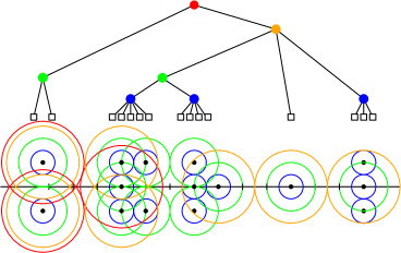
Figure 3: A dense pointset $P$ and construction of ${\cal T}_{P}$. Circles of different colors correspond to different $\sigma$’s. The first choice of $\sigma$ corresponds to blue colored circles, followed by green, orange and red. The components formed are shown in the corresponding colors. We only draw some of the relevant circles to give an idea.

Let $u,v\in{\cal T}_{P}$ be such that $v$ is a child of $u$. We have the following properties of ${\cal T}_{P}$:

1. $\sigma_{u}\leq\min_{p\in G_{v},q\in P\setminus G_{v}}|p-q|\leq 3r_{v}$. The upper bound follows from the density of $P$. The lower bound follows from the observation that the discs with radius $\sigma/2$ centered at $p\in G_{v}$, where $\sigma_{v}<\sigma<\sigma_{u}$, do not touch the discs of any other component, except when the radius is $\sigma_{u}/2$.

2. $r_{u}\leq|G_{u}|\sigma_{u}$. Consider the graph ${\cal G}$ with the vertices as $G_{u}$ and edges between two vertices $p,q$ if $D(p,\sigma_{u}/2)\cap D(q,\sigma_{u}/2)\neq\emptyset$. As $G_{u}$ is a connected component of these discs, we know that ${\cal G}$ is connected. Therefore, if $m$ is the number of vertices on the path joining $p,q$ in ${\cal G}$, then by triangular inequality $|p-q|\leq m\sigma_{u}\leq|G_{u}|\sigma_{u}$.

3. If $p$ is a leaf-child of $u$ then $\sigma_{u}=\sigma_{p}$. It is clear that any disc $D(p,r)$, with $r<\sigma_{p}/2$, cannot touch $D(q,r)$, for any other point $q$. The first time they touch is when $\sigma_{u}=\sigma_{p}$. If $p\in{\mathbb{C}}\setminus{\mathbb{R}}$, then we further obtain that $|\mbox{\tt Im}(p)|\geq\sigma_{p}\geq\sigma_{u}$.

4. The size of ${\cal T}_{P}=O(|P|)$. Every level has a node with more than one child, as there are pairs of components with separation exactly $\sigma$.

5. $P$ is the component associated with the root of ${\cal T}_{P}$.

The next result is an amortization analogous to that of the Davenport-Mahler bound over the root separation bound.

Lemma 12.

If $P$ is a dense pointset then

$$\int_{(2D_{P}\cap{\mathbb{R}})\setminus\cup_{p\in P}J_{p}}\frac{dx}{d(x,P)}=O(|P|\ln|P|),$$ (16)

where for $p\in P\cap{\mathbb{R}}$, $J_{p}{\color[rgb]{1,0,0}\mathrel{\,:=\,}}[p\pm\sigma_{p}/2]$, and $J_{p}=\emptyset$ otherwise.

Proof. We break the integral recursively over the nodes of ${\cal T}_{P}$. For an internal node $u$ of ${\cal T}_{P}$, we will show the following claim:

$$\int_{(2D(G_{u})\cap{\mathbb{R}})\setminus\cup_{p\in G_{u}}J_{p}}\frac{dx}{d(x,P)}=O(\nu_{u}\ln|G_{u}|).$$ (17)

We take the sum over all internal nodes $u$. From (P4) we know that $|{\cal T}_{P}|=O(|P|)$, and hence $\sum_{u}\nu_{u}=O(|P|)$; moreover, from (P5) we know that the component associated with the root of ${\cal T}_{P}$ is $P$. These observations then give us (16).

For a point $p\in P$, recall that ${\cal V}_{p}$ is the set of points in $2D_{P}\cap{\mathbb{R}}$ closer to $p$ than to any other point of $P$; by definition $J_{p}\subseteq{\cal V}_{p}$. Suppose $u$ is the parent of $p$. We will bound the integral over ${\cal V}_{p}$ in two steps: the portion of ${\cal V}_{p}$ inside $2D(G_{u})$ and the portion outside $2D(G_{u})$. The latter portion is where amortization occurs, as for an $x\not\in 2D(G_{u})$, the distance of $x$ to $p\in G_{u}$ is roughly $|x-m_{u}|$. Let $v$ be a child of $u$. There are three cases to consider:

1. Case 1. $v$ is a leaf $p\in{\mathbb{R}}$. We first bound the portion $I_{p}$ of ${\cal V}_{p}$ inside $2D(G_{u})$; the portion outside will be handled collectively for all points in the third case. For all $x\in I_{p}\setminus J_{p}$, it is clear that $d(x,P)=|x-p|$. From Lemma 11(Re) we obtain that $\int_{I_{p}\setminus J_{p}}\frac{dx}{|x-p|}=O\left({\ln\frac{w(I_{p})}{\sigma_{p}}}\right)$. But as $I_{p}\subseteq 2D(G_{u})\cap{\mathbb{R}}$, we know that $w(I_{p})\leq 4r_{u}$. From (P3), we know that $\sigma_{p}=\sigma_{u}$. Therefore, $\int_{I_{p}\setminus J_{p}}\frac{dx}{|x-p|}=O(\ln r_{u}/\sigma_{u})=O(\ln|G_{u}|)$, from (P2).

2. Case 2. $v$ is a leaf $p=\mbox{\tt Re}(p)+i\mbox{\tt Im}(p)\in{\mathbb{C}}\setminus{\mathbb{R}}$. Again consider the interval $I_{p}{\color[rgb]{1,0,0}\mathrel{\,:=\,}}{\cal V}_{p}\cap 2D(G_{u})$; in this case $J_{p}=\emptyset$. As $p$ is the closest point to any $x\in I_{p}$, $d(x,P)=|x-p|$. Moreover, $p$ and both the endpoints of $I_{p}$ are in $2D(G_{u})$, so the maximum distance of an endpoint of $I_{p}$ from $p$ is $\leq 2r_{u}$. Therefore, from Lemma 11(Im) we have

   $$\int_{I_{p}}\frac{dx}{d(x,P)}=O\left({\ln\frac{r_{u}}{|\mbox{\tt Im}(p)|}}\right).$$

   But recall from (P3) that $|\mbox{\tt Im}(p)|\geq\sigma_{u}$, hence $r_{u}/|\mbox{\tt Im}(p)|\leq r_{u}/\sigma_{u}\leq|G_{u}|$, where the last inequality follows from (P2). Therefore, $\int_{I_{p}}\frac{dx}{d(x,P)}=O(\ln|G_{u}|)$.

3. Case 3. $v$ is an internal node. Inductively, we have already bounded the integral $\int_{(2D(G_{v})\cap{\mathbb{R}})\setminus\cup_{p\in G_{v}}J_{p}}dx/d(x,P)$. However, it is possible that ${\cal V}_{p}$, for some point $p\in G_{v}$ extends beyond $2D(G_{v})\cap{\mathbb{R}}$. Suppose $p$ is such a point, and $x\in W_{p}{\color[rgb]{1,0,0}\mathrel{\,:=\,}}{\cal V}_{p}\cap(2D(G_{u})\setminus 2D(G_{v}))$. Then we know that $|x-p|\geq|x-m_{v}|/2$, where $m_{v}$ is the center of $D(G_{v})$. Therefore,

   $$\sum_{p\in G_{v}}\int_{W_{p}}\frac{dx}{|x-p|}\leq\int_{(2D(G_{u})\setminus 2D(G_{v}))\cap{\mathbb{R}}}\frac{2dx}{|x-m_{v}|}.$$

   As $2w(I_{u})=4r_{u}$, from Lemma 11(Re), it follows that the integral on the RHS is bounded by $O(\ln r_{u}/r_{v})$. But from (P2) we have $r_{u}\leq|G_{u}|\sigma_{u}$, and $\sigma_{u}\leq 3r_{v}$ from (P1). Therefore, we obtain

   $$\sum_{p\in G_{v}}\int_{W_{p}}\frac{dx}{d(x,P)}=O(|\ln|G_{u}|).$$

   This is the case where the amortization of the integral over the Voronoi regions takes place.

Summing the bounds for all children $v$ of $u$ gives (17).   Q.E.D.

The following is the analogue of Lemma 12 in ${\mathbb{C}}$: define $D_{p}{\color[rgb]{1,0,0}\mathrel{\,:=\,}}D(p,\sigma_{p}/2)$, then

$$\int_{2D_{P}\setminus\cup_{p}D_{p}}\frac{dz}{d(z,P)}=O(|P|\ln|P|).$$

5 Concluding Remarks

Our aim has been to devise a general approach to improve any subdivision based algorithm for real root isolation. This is achieved by the Newton-Incl-Exc predicate, which detects strongly separated clusters, and hence reduces the number of subdivisions from $O(\log R_{\cal C}/r_{\cal C})$ to $O(n\log n)$. The crucial ingredient is Ostrowski’s criterion based on deviations of the Newton diagram of a polynomial. The criterion works for complex polynomials, so we expect an analogue of Newton-Isol for isolating complex roots that is conceptually simpler than the existing approaches. We have not explored the practical aspects of the algorithm, nevertheless, we think that the analysis based on the geometry of cluster provides tools and techniques for an alternate approach to understand existing algorithms.

We can bound the arithmetic complexity of Newton-Isol as follows. The Newton diagram computation takes $O(n)$, and the Taylor shift $O(n\log n)$ operations. The number of Newton iterations to approximate ${\cal C}$ is bounded by $O(\log\log\frac{R_{\cal C}}{r_{\cal C}})$, which is $O(\log(nL))$ from root separation bounds. Therefore, the arithmetic complexity, ignoring poly-log factors, is bounded by $\widetilde{O}(n^{2})$. The extension to the bitstream model involves deriving a robust version of Ostrowski’s result and bounding precision requirements. The latter will be governed by perturbation bounds for clusters. For a cluster of size $k$, we expect these bounds to be $O(\epsilon^{1/k})$, for $\epsilon$-perturbation in the coefficients. In the worst case, this would give an $O(n(L+\log n))$ bound on the precision.

Appendix

We give the proof of Lemma 3; the arguments are based standard manipulations with Taylor series in alpha-theory of Smale et al. We first prove Lemma 3(i), for which we need the following functions from [BCSS98] defined for $f^{(k-1)}$:

$$\beta_{k}(z)=\left\lvert\frac{f^{(k-1)}(z)}{f^{(k)}(z)}\right\rvert,\;\gamma_{k}(z)=\max_{j\geq 1}\left\lvert\frac{f^{(k+j)}(z)}{(j+1)!f^{(k)}(z)}\right\rvert^{\frac{1}{j}}$$ (18)

and $\alpha_{k}(z)=\beta_{k}(z)\gamma_{k}(z)$. We derive relations between these quantities and $\rho_{k}(z)$’s given in (2). Considering the RHS of $\rho_{k}(z)$ for $j=k-1$, we immediately have

$$\rho_{k}(z)\geq\left\lvert\frac{f_{k-1}(z)}{f_{k}(z)}\right\rvert=k\beta_{k}(z).$$ (19)

Multiplying and dividing the inner term on the RHS of $\gamma_{k}(z)$ in (18) by $(k+j)!/k!$ we obtain that

$$\gamma_{k}(z) \leq\max_{j\geq 1}\left({\frac{(k+j)!}{k!(j+1)!}}\right)^{1/j}\max_{j>k}\left\lvert\frac{f_{j}(z)}{f_{k}(z)}\right\rvert^{1/(j-k)}$$

$$=\max_{j\geq 1}\left({\frac{(k+j)!}{k!(j+1)!}}\right)^{1/j}\frac{1}{\rho_{k+1}(z)}.$$

The max-term is bounded by $(k+1)$, which implies that

$$\gamma_{k}(z)\rho_{k+1}(z)\leq(k+1).$$ (20)

Multiplying (19) and (20) we obtain that $\alpha_{k}(z)\Delta_{k}(z)\leq 2.$ Therefore, if $\Delta_{k}(z)\geq 12$ then $z$ is an approximate zero of $f^{(k-1)}$ with associated root in $D(z,1.5\beta_{k}(z))\subseteq D(z,\frac{3\rho_{k}(z)}{2k})$, where the inclusion follows from (19). The claim on Newton iterates follows from [BCSS98, p. 160,Thm.2].

We now prove Lemma 3(ii). We will need the following result [BCSS98, p. 161, Lem. 3]: for a $u\in[0,1)$

$$\sum_{j\geq 0}{k+j\choose j}u^{j}=\frac{1}{(1-u)^{k+1}}.$$ (21)

Let $\epsilon{\color[rgb]{1,0,0}\mathrel{\,:=\,}}1.5$, $\delta{\color[rgb]{1,0,0}\mathrel{\,:=\,}}\epsilon\rho_{k}/k$, and $u{\color[rgb]{1,0,0}\mathrel{\,:=\,}}\frac{\delta}{\rho_{k+1}}=\frac{\epsilon}{k\Delta_{k}}$; here we express $\rho_{k}(z)$ by $\rho_{k}$ (similarly, for the other quantities).

Lemma 13.

If $z$ is such that $\Delta_{k}(z)\geq 16$ then for $z^{\prime}\in D(z,\delta)$, we have $|f_{k}(z^{\prime})|\geq|f_{k}(z)|(1-u)^{-(k+1)}/2$.

Proof. Take the absolute values in the Taylor expansion of $f^{(k)}(z^{\prime})$ and apply the triangular inequality to obtain

$$\left\lvert f_{k}(z^{\prime})\right\rvert\geq\frac{1}{k!}\left({|f^{(k)}(z)|-\sum_{j\geq 1}\left\lvert\frac{f^{(k+j)}(z)}{j!}\right\rvert\delta^{j}}\right).$$

Dividing both sides by $|f_{k}(z)|$, and multiplying and dividing the summation term on the RHS by $k!$ and $(k+j)!$ we obtain that

$$\left\lvert\frac{f_{k}(z^{\prime})}{f_{k}(z)}\right\rvert\geq\left({1-\sum_{j\geq 1}{k+j\choose j}\left\lvert\frac{f_{k+j}(z)}{f_{k}(z)}\right\rvert\delta^{j}}\right).$$

From the expression of $\rho_{k+1}(z)$ in (2) and definition of $u$, we deduce that

$$\left\lvert\frac{f_{k}(z^{\prime})}{f_{k}(z)}\right\rvert \geq\left({2-\sum_{j\geq 0}{k+j\choose j}u^{j}}\right).$$

Using (21), and the bound on $\Delta_{k}$, the RHS can be simplified to $(1-u)^{-(k+1)}/2$.   Q.E.D.

Lemma 14.

If $\Delta_{k}(z)\geq 16$ then for all $z^{\prime}\in D(z,\delta)$ we have $\rho_{k}(z^{\prime})<2e^{6}\rho_{k}(z)$ and $\rho_{k+1}(z^{\prime})\geq\rho_{k+1}(z)/3$. Therefore, $\Delta_{k}(z^{\prime})\geq\Delta_{k}(z)/(6e^{6})$.

Proof. For $j<k$, take absolute values in the Taylor expansion of $f_{j}(z^{\prime})$, apply triangular inequality, and split the summation up to $k$ and beyond $k$, to get

$$|f_{j}(z^{\prime})|=|f_{j}(z)|+\sum_{\ell=1}^{k-j}{\ell+j\choose\ell}\left\lvert{f_{\ell+j}(z)}\right\rvert\delta^{\ell}+\sum_{\ell>k-j}{\ell+j\choose\ell}\left\lvert f_{\ell+j}(z)\right\rvert\delta^{\ell}.$$

Divide by $|f_{k}(z)|$ and use the expressions in (2) to obtain

$$\left\lvert\frac{f_{j}(z^{\prime})}{f_{k}(z)}\right\rvert\leq\rho_{k}^{k-j}+\sum_{\ell=1}^{k-j}{\ell+j\choose\ell}\rho_{k}^{k-\ell-j}\delta^{\ell}+\sum_{\ell>k-j}{\ell+j\choose\ell}\frac{\delta^{\ell}}{\rho_{k+1}^{\ell+j-k}}.$$

Since $\delta=\epsilon\rho_{k}/k$, we can pull out $\rho_{k}^{k-j}$ from the RHS (and since $\Delta_{k}>1$), we get that

$$\left\lvert\frac{f_{j}(z^{\prime})}{f_{k}(z)}\right\rvert\leq\rho_{k}^{k-j}\left({1+\sum_{\ell=1}^{k-j}{\ell+j\choose\ell}\left({\frac{\epsilon}{k}}\right)^{\ell}+\sum_{\ell>k-j}{\ell+j\choose\ell}\left({\frac{\epsilon}{k}}\right)^{\ell}}\right).$$

Assuming $k\geq 2$, from (21) we obtain that

$$\left\lvert\frac{f_{j}(z^{\prime})}{f_{k}(z)}\right\rvert\leq\rho_{k}^{k-j}\left({1-\frac{\epsilon}{k}}\right)^{-(j+1)}.$$

Combining this bound with Lemma 13, and doing some further simplifications we obtain the upper bound on $\rho_{k}(z^{\prime})$. Note that we require $k\geq 2>\epsilon$. To derive a lower bound on $\rho_{k+1}(z^{\prime})$ in terms of $\rho_{k+1}(z)$, we take absolute values in the Taylor expansion of $f_{j}(z^{\prime})$, for $j>k$, apply the triangular inequality, and divide both sides by $|f_{k}(z)|$, to get

$$\left\lvert\frac{f_{j}(z^{\prime})}{f_{k}(z)}\right\rvert\leq\left\lvert\frac{f_{j}(z)}{f_{k}(z)}\right\rvert+\sum_{\ell\geq 1}{\ell+j\choose\ell}\left\lvert\frac{f_{\ell+j}(z)}{f_{k}(z)}\right\rvert\delta^{\ell}.$$

From the expression for $\rho_{k+1}$ in (2) and (21) it follows that

$$\left\lvert\frac{f_{j}(z^{\prime})}{f_{k}(z)}\right\rvert\leq\frac{1}{\rho_{k+1}^{j-k}}\left({1-u}\right)^{-(j+1)}.$$

Combining this with the lower bound in Lemma 13, and using the lower bound on $\Delta_{k}$ we further obtain that

$$\left\lvert\frac{f_{j}(z^{\prime})}{f_{k}(z^{\prime})}\right\rvert^{1/(j-k)}\leq\frac{2^{j-k}}{(1-u)\rho_{k+1}}.$$

Since $u\leq\epsilon/(k\Delta_{k})$ and $\Delta_{k}\geq 16$, we get that

$$\left\lvert\frac{f_{j}(z^{\prime})}{f_{k}(z^{\prime})}\right\rvert^{1/(j-k)}\leq\frac{3}{\rho_{k+1}},$$

which implies the desired lower bound on $\rho_{k+1}(z^{\prime})$.   Q.E.D.

To show Lemma 3(iii), we suppose that $\rho_{k}(w)\leq\rho_{k}(z)$. As the two inclusion discs intersect it follows that

$$|w\pm 3\rho_{k}(w)-z|\leq|z-w|+3\rho_{k}(w)\leq 9\rho_{k}(z)\leq\frac{\rho_{k+1}(z)}{3},$$

where the last inequality follows from $\Delta_{k}(z)\geq 27$. This implies that $D(w,3\rho_{k}(w))\subseteq D(z,\frac{\rho_{k+1}(z)}{3})$, and hence both the discs have the same cluster.

We next give a self-contained proof of Pawlowski’s result [Paw99, Thm. 2.2]. The difference in our proof is that we avoid using Eneström-Kakeya theorem. The key idea of using Walsh’s representation theorem [RS02, Thm. 3.4.1c], however, is common to both the proofs.

Given a cluster ${\cal C}$ of size $k$, and $z\in{\mathbb{C}}$, let $f_{1}(z)={\tt lead}(f)\prod_{\alpha\in{\cal C}}(z-\alpha)$ and $f_{2}(z)=\prod_{\beta\in\overline{{\cal C}}}(z-\beta)$. From Leibniz’s formula we have

$$f^{(j)}(z)=\sum_{i=\max\left\{0,j+k-n\right\}}^{\min\left\{j,k\right\}}{j\choose i}f_{1}^{(i)}(z)f_{2}^{(j-i)}(z).$$

We will focus on the case when $j\leq k$, in which case the upper bound of the summation is $j$. The bounds on the summation are required because $f_{1}$ cannot be differentiated more than $k$ times and similarly for $f_{2}$. Applying Walsh’s representation theorem, first to $f_{1}$ we obtain that there is an $\alpha\in D(m,r_{\cal C})$ such that

$$f^{(j)}(z)=\sum_{i=\max\left\{0,j+k-n\right\}}^{j}{j\choose i}k(k-1)\cdots(k-i+1)(z-\alpha)^{k-i}f_{2}^{(j-i)}(z).$$

Now applying Walsh’s representation theorem to $f_{2}$, we know that there is a $\beta\not\in D(m,R_{\cal C})$ such that

$$f^{(j)}(z)=\sum_{i=\max\left\{0,j+k-n\right\}}^{j}{j\choose i}k(k-1)\cdots(k-i+1)(z-\alpha)^{k-i}(n-k)(n-k-1)\cdots(n-k-j+i+1)(z-\beta)^{n-k-j+i}.$$

Opening up the binomial ${j\choose i}$ and simplifying we obtain

$$f_{j}(z)=\frac{f^{(j)}(z)}{j!}=\sum_{i=\max\left\{0,j+k-n\right\}}^{j}{k\choose i}(z-\alpha)^{k-i}{n-k\choose j-i}(z-\beta)^{n-k-j+i}.$$

Pulling out the last term from the RHS we obtain that

$$f_{j}(z)={k\choose j}(z-\alpha)^{k-j}(z-\beta)^{n-k}\sum_{i=\max\left\{0,j+k-n\right\}}^{j}\frac{{k\choose i}{n-k\choose j-i}}{{k\choose j}}\left({\frac{z-\alpha}{z-\beta}}\right)^{j-i};$$

note that when $j=k$, the term $(z-\alpha)^{k-j}$ is one. Now we substitute $i$ by $j-i$ to obtain

$$f_{j}(z)={k\choose j}(z-\alpha)^{k-j}(z-\beta)^{n-k}\sum_{i=0}^{\min\left\{j,n-k\right\}}\frac{{k\choose j-i}{n-k\choose i}}{{k\choose j}}\left({\frac{z-\alpha}{z-\beta}}\right)^{i}.$$ (22)

The fraction

$$\frac{{k\choose j-i}{n-k\choose i}}{{k\choose j}}=\frac{1}{i!}\frac{(n-k)!}{(n-k-i)!}\frac{j!}{(j-i)!}\frac{(k-j)!}{(k-j+i)!}\leq\frac{1}{i!}\left({\frac{(n-k)j}{(k-j)}}\right)^{i};$$

note that for $j=k$, the denominator does not appear; we capture this by using the notation $(x)_{1}{\color[rgb]{1,0,0}\mathrel{\,:=\,}}\max\left\{1,x\right\}$. Therefore, the summation in (22) does not vanish if $z$ satisfies the following inequality:

$$\frac{1}{2}\geq\sum_{i\geq 1}^{\min\left\{j,n-k\right\}}\frac{1}{i!}\left({\frac{j(n-k)}{(k-j)_{1}}\left\lvert\frac{z-\alpha}{z-\beta}\right\rvert}\right)^{i}.$$

Substituting the upper bound of the summation by infinity, we get the following stronger constraint:

$$\frac{1}{2}\geq\sum_{i\geq 1}\frac{1}{i!}\left({\frac{j(n-k)}{(k-j)_{1}}\left\lvert\frac{z-\alpha}{z-\beta}\right\rvert}\right)^{i}.$$

Adding one on both sides, and using the observation that the RHS is the expansion of $\exp(\left({\frac{j(n-k)}{(k-j)_{1}}\left\lvert\frac{z-\alpha}{z-\beta}\right\rvert}\right))$, we get that the inequality follows if

$$\ln 1.5\geq\frac{1}{4}\geq\left({\frac{j(n-k)}{(k-j)_{1}}\left\lvert\frac{z-\alpha}{z-\beta}\right\rvert}\right).$$ (23)

Since $\alpha\in D(m_{\cal C},r_{\cal C})$, we have

$$|z-\alpha|\leq|z-m_{\cal C}|+r_{\cal C}\leq 2\max(|z-m_{\cal C}|,r_{\cal C}),$$

and

$$|z-\beta|\geq|m_{\cal C}-\beta|-|z-m_{\cal C}|\geq R_{\cal C}-|z-m_{\cal C}|\geq R_{\cal C}-\max\left\{|z-m_{\cal C}|,r_{\cal C}\right\}.$$

These bounds imply that

$$\frac{|z-\alpha|}{|z-\beta|}\leq 2\frac{\max\left\{|z-m_{\cal C}|,r_{\cal C}\right\}}{(R_{\cal C}-\max\left\{|z-m_{\cal C}|,r_{\cal C}\right\})},$$

and hence (23) follows if

$$R_{\cal C}\geq\max\left\{|z-m_{\cal C}|,r_{\cal C}\right\}\left({1+\frac{8j(n-k)}{(k-j)_{1}}}\right).$$

To summarize, we have the following result:

Lemma 15.

Let ${\cal C}$ be a cluster of size $k$ and $j\in\left\{0,\ldots,k\right\}$. If $z\in{\mathbb{C}}$ is such that

$$R_{\cal C}\geq 2\max\left\{|z-m_{\cal C}|,r_{\cal C}\right\}\left({\frac{8j(n-k)}{(k-j)_{1}}}\right)_{1},$$ (24)

then

$$f_{j}(z)={k\choose j}(z-\alpha)^{k-j}(z-\beta)^{n-k}(1\pm\frac{1}{2}),$$

for some $\alpha\in D(m,r_{\cal C})$ and $\beta\not\in D(m,R_{\cal C})$; the notation “$\pm$” stands for a $\theta\in{\mathbb{C}}$ such that $|\theta|\leq 1$. Moreover, if $z$ also satisfies $|z-m_{\cal C}|>r_{\cal C}$ then $f^{(j)}(z)\neq 0$.

We specialize this result to the case of a strongly separated cluster:

Corollary 16.

For a strongly separated cluster ${\cal C}$, if $z$ is such that

$$|z-m_{\cal C}|\leq\frac{R_{\cal C}}{4n^{2}}$$

then for $0\leq j\leq k$,

$$f_{j}(z)={k\choose j}(z-\alpha)^{k-j}(z-\beta)^{n-k}(1\pm\frac{1}{2}),$$

for some $\alpha\in D(m,r_{\cal C})$ and $\beta\not\in D(m,R_{\cal C})$. Moreover, if $z$ also satisfies $|z-m_{\cal C}|>r_{\cal C}$ then $f^{(j)}(z)\neq 0$, for $0\leq j\leq k$.

Proof. Note that the maximum value of the term $j(n-k)/(k-j)_{1}$ is obtained at $j=k$, and it is $k(n-k)$. From the AM-GM inequality, we know that $k(n-k)\leq n^{2}/4$. Therefore, (24) follows if $z$ and $r_{\cal C}$ are such that

$$R_{\cal C}\geq 4n^{2}\max\left\{|z-m_{\cal C}|,r_{\cal C}\right\}.$$

For a strongly separated cluster ${\cal C}$ we know that $R_{\cal C}\geq 4n^{2}r_{\cal C}$, and the condition on $z$ is the condition in the corollary.   Q.E.D.

We use this result to show that $(k-j)$ roots of the $j$th derivative are in $D(m_{\cal C},r_{\cal C})$ and the remaining are outside $D(m_{\cal C},R_{\cal C}/(2n^{2}))$. Let $\alpha_{1},\ldots,\alpha_{k}$ be the roots of $f$ in ${\cal C}$ and let $\beta_{1},\ldots,\beta_{n-k}$ be the remaining roots. Let $g_{t}$ be the polynomial with roots $(1-t)m_{\cal C}+t\alpha_{1},\ldots,(1-t)m_{\cal C}+t\alpha_{k},\beta_{1},\ldots,\beta_{n-k}$. Thus $g_{0}(z)=(z-m_{\cal C})^{k}\prod_{\beta\in\overline{{\cal C}}}(z-\beta)$ and $g_{1}(z)=f(z)$. Since $g_{t}(z)$ has a strongly separated cluster of size $k$ in $D(m_{\cal C},tr_{\cal C})$, from the lemma above we know that $g_{t}^{(j)}(z)$ does not vanish on the boundary of $D(m_{\cal C},r_{\cal C})$. As the roots vary continuously with $t$, and $g_{0}^{(j)}(z)$ has a root of multiplicity $(k-j)$ at $m_{\cal C}$, it follows that $g_{t}^{(j)}(z)$ has $k-j$ roots in $D(m_{\cal C},tr_{\cal C})$ and the remaining roots outside $D(m_{\cal C},R_{\cal C}/(2n^{2}))$. Substituting $t=1$ gives us the desired result. To summarize, we have obtained the following result:

Lemma 17.

Given a strongly separated cluster ${\cal C}$ of size $k$, for $j\leq k$, there are $k-j$ roots of the derivative $f^{(j)}(z)$ in $D(m_{\cal C},r_{\cal C})$ and the remaining $(n-k)$ roots are outside $D(m_{\cal C},R_{\cal C}/(2n^{2}))$.

References

- [BCSS98] Lenore Blum, Felipe Cucker, Michael Shub, and Steve Smale. Complexity and Real Computation. Springer-Verlag, New York, 1998.
- [BKY09] Michael Burr, Felix Krahmer, and Chee Yap. Continuous amortization: A non-probabilistic adaptive analysis technique. Electronic Colloquium on Computational Complexity (ECCC), TR09(136), December 2009.
- [Bur13] Michael A. Burr. Applications of continuous amortization to bisection-based root isolation. CoRR, abs/1309.5991, 2013.
- [CA76] George E. Collins and Alkiviadis G. Akritas. Polynomial real root isolation using Descartes’ rule of signs. In R. D. Jenks, editor, Proceedings of the 1976 ACM Symposium on Symbolic and Algebraic Computation, pages 272–275. ACM Press, 1976.
- [Dav85] James H. Davenport. Computer algebra for cylindrical algebraic decomposition. Tech. Rep., The Royal Inst. of Technology, Dept. of Numerical Analysis and Computing Science, S-100 44, Stockholm, Sweden, 1985. Reprinted as Tech. Report 88-10 , School of Mathematical Sci., U. of Bath, Claverton Down, Bath BA2 7AY, England. URL http://www.bath.ac.uk/~masjhd/TRITA.pdf.
- [ESY06] Arno Eigenwillig, Vikram Sharma, and Chee Yap. Almost tight complexity bounds for the Descartes method. In 31st Int’l Symp. Symbolic and Alge. Comp. (ISSAC), pages 71–78, 2006. Genova, Italy. Jul 9-12, 2006.
- [GLSY05] M. Giusti, G. Lecerf, B. Salvy, and J.-C. Yakoubsohn. On location and approximation of clusters of zeros of analytic functions. Found. Comput. Math., 5(3):257–311, July 2005.
- [Ost40] Alexandre Ostrowski. Recherches sur la méthode de Graeffe et les zéros des polynomes et des séries de Laurent. Acta Mathematica, 72:99–155, 1940.
- [Pan00] Victor Y. Pan. Approximating complex polynomial zeros: Modified Weyl’s quadtree construction and improved newton’s iteration. J. Complexity, 16(1):213–264, 2000.
- [Paw99] Piotr Pawlowski. The location of the zeros of the higher order derivatives of a polynomial. Proceedings of the American Mathematical Society, 127(5):1493–1497, 1999.
- [RS02] Qazi Ibadur Rahman and Gerhard Schmeisser. Analytic Theory of Polynomials. Oxford University Press, 2002.
- [Sag12] Michael Sagraloff. When Newton meets Descartes: a simple and fast algorithm to isolate the real roots of a polynomial. In Joris van der Hoeven and Mark van Hoeij, editors, International Symposium on Symbolic and Algebraic Computation, ISSAC’12, Grenoble, France - July 22 - 25, 2012, pages 297–304. ACM, 2012.
- [Sha11] Meisam Sharify. Scaling Algorithms and Tropical Methods in Numerical Matrix Analysis. PhD thesis, Centre de Mathematique Appliqué, Ecole Polytechnique & INRIA Saclay, 2011.
- [SM13] Michael Sagraloff and Kurt Mehlhorn. Computing real roots of real polynomials - an efficient method based on Descartes’ rule of signs and Newton iteration. CoRR, abs/1308.4088, 2013.
- [SSY13] Michael Sagraloff, Vikram Sharma, and Chee Yap. Analytic root clustering: A complete algorithm using soft zero tests. In Paola Bonizzoni, Vasco Brattka, and Benedikt Löwe, editors, The Nature of Computation. Logic, Algorithms, Applications - 9th Conference on Computability in Europe, CiE 2013, Milan, Italy, July 1-5, 2013. Proceedings, volume 7921 of Lecture Notes in Computer Science, pages 434–444. Springer, 2013.
- [ST09] Tateaki Sasaki and Akira Terui. Computing clustered close-roots of univariate polynomials. In Hiroshi Kai, Hiroshi Sekigawa, Tateaki Sasaki, Kiyoshi Shirayanagi, and Ilias S. Kotsireas, editors, Symbolic Numeric Computation, SNC ’09, Kyoto, Japan - August 03 - 05, 2009, pages 177–184. ACM, 2009.
- [SY12] Vikram Sharma and Chee-Keng Yap. Near optimal tree size bounds on a simple real root isolation algorithm. In Joris van der Hoeven and Mark van Hoeij, editors, 37th Int’l Symp. Symbolic and Alge. Comp. (ISSAC), pages 319–326. ACM, 2012. Grenoble, France - July 22 - 25, 2012.
- [Yak00] Jean-Claude Yakoubsohn. Simultaneous computation of all the zero-clusters of a univariate polynomial. In Felipe Cucker and J. Maurice Rojas, editors, Proceedings of the SMALEFEST, Foundations of Computational Mathematics (Hong Kong), pages 433–455, Singapore, 2000. World Scientific.