A realizability-preserving high-order kinetic scheme using WENO reconstruction for entropy-based moment closures of linear kinetic equations in slab geometry

Abstract

We develop a high-order kinetic scheme for entropy-based moment models of a one-dimensional linear kinetic equation in slab geometry. High-order spatial reconstructions are achieved using the weighted essentially non-oscillatory (WENO) method, and for time integration we use multi-step Runge-Kutta methods which are strong stability preserving and whose stages and steps can be written as convex combinations of forward Euler steps. We show that the moment vectors stay in the realizable set using these time integrators along with a maximum principle-based kinetic-level limiter, which simultaneously dampens spurious oscillations in the numerical solutions. We present numerical results both on a manufactured solution, where we perform convergence tests showing our scheme converges of the expected order up to the numerical noise from the numerical optimization, as well as on two standard benchmark problems, where we show some of the advantages of high-order solutions and the role of the key parameter in the limiter.

1 Introduction

In recent years many approaches have been considered for the solution of time-dependent linear kinetic transport equations, which arise for example in electron radiation therapy or radiative heat transfer problems. Many of the most popular methods are moment methods, also known as moment closures because they are distinguished by how they close the truncated system of exact moment equations. Moments are defined through angular averages against basis functions to produce spectral approximations in the angle variable. A typical family of moment models are the so-called P_N-methods [25, 16] which are pure spectral methods. However, many high-order moment methods, including P_N, do not take into account that the original kinetic density to be approximated must be nonnegative. The moment vectors produced by such models are therefore often not realizable, that is, there is no associated nonnegative kinetic density consistent with the moment vector, and thus the solutions can contain obviously non-physical artifacts such as negative local particle densities [6].

The family of minimum-entropy models, colloquially known as $\text{M}_{N}$ models or entropy-based moment closures, solve this problem (for certain physically relevant entropies) by specifying the closure using a nonnegative density reconstructed from the moments. The $\text{M}_{N}$ models are the only models which additionally are hyperbolic and dissipate entropy [24]. The cost of all these properties is that the reconstruction of this density involves solving an optimization problem at every point on the space-time mesh. These reconstructions, however, can be parallelized, and so the recent emphasis on algorithms that can take advantage of massively parallel computing environments has led to renewed interest in the computation of $\text{M}_{N}$ solutions both for linear and nonlinear kinetic equations [10, 18, 21, 2, 15, 27]. Despite the parallelizability of the cost of the numerical optimization, the gain in efficiency that would come from a higher-order space-time discretization will still be necessary for a practical $\text{M}_{N}$ implementation.

The key challenge for high-order methods for entropy-based moment closures is that the numerical solutions leave the set of realizable moments [28], outside of which the defining optimization problem has no solution. Discontinuous-Galerkin methods can handle this problem using a realizability limiter directly on the moment vectors themselves [39, 28, 4], but at this level realizability conditions are in general quite complicated and also not well-understood for two- or three-dimensional problems for moment models of order higher than two. Realizability limiting for kinetic schemes, however, is much easier because at the level of the kinetic density, realizability corresponds simply to nonnegativity. Furthermore, this same limiter can be strengthened to also enforce a local maximum principle, thereby dampening artificial oscillations in numerical solutions.

Thus in this work we derive a high-order (in space and time) kinetic scheme for $\text{M}_{N}$ models with moments of (in principle) arbitrary order. We start in Section 2 by introducing the linear kinetic equation we will consider, its entropy-based moment closure, and reviewing the concept of realizability. Continuing in Section 3 we introduce the concept of a kinetic scheme for moment equations and then give our numerical techniques for the discretization of each of the independent variables: angle, space, and time. The issue of realizability preservation and the necessary limiters are discussed in Section 4, finishing the full description of our scheme. The results from our numerical simulations are presented in Section 5, including a convergence study using a manufactured solution and solutions for two benchmark problems. Finally we draw conclusions and discuss the next steps for future work in Section 6.

2 A linear kinetic equation and moment closures

We begin with the linear kinetic equation we will use to test our algorithm and a brief introduction to entropy-based moment closures which closely follows [4]. More background can be found for example in [25, 24, 18] and references therein.

2.1 A linear kinetic equation

We consider the following one-dimensional linear kinetic equation for the kinetic density $\psi=\psi(t,x,\mu)\geq 0$ in slab geometry, for time $t>0$, spatial coordinate $x\in X=(x_{\text{L}},x_{\text{R}})\subseteq\mathbb{R}$, and angle variable $\mu\in[-1,1]$:

$$\partial_{t}\psi+\mu\partial_{x}\psi+\sigma_{\mathrm{a}}\psi=\sigma_{\mathrm{s}}\mathcal{C}(\psi)+S,$$ (2.1)

where $\sigma_{\mathrm{a}}$ and $\sigma_{\mathrm{s}}$ are the nonnegative absorption and scattering interaction coefficients, and $S$ a source. The operator $\mathcal{C}$ is a collision operator, which in this paper we assume to be linear and have the form

$$\mathcal{C}(\psi)=\int_{-1}^{1}T(\mu,\mu^{\prime})\psi(t,x,\mu^{\prime})~{}d\mu^{\prime}-\int_{-1}^{1}T(\mu^{\prime},\mu)\psi(t,x,\mu)~{}d\mu^{\prime}.$$ (2.2)

We assume that the kernel $T$ is strictly positive and normalized to $\int_{-1}^{1}T(\mu^{\prime},\mu)d\mu^{\prime}~{}\equiv~{}1$. A typical example is isotropic scattering, where $T(\mu,\mu^{\prime})\equiv 1/2$.

Equation (2.1) is supplemented by initial and boundary conditions:

$$\psi(t,x_{\text{L}},\mu) =\psi_{\text{L}}(t,\mu)\,, t \geq 0\,, \mu >0\,,$$ (2.3a)

$$\psi(t,x_{\text{R}},\mu) =\psi_{\text{R}}(t,\mu)\,, t \geq 0\,, \mu <0\,,$$ (2.3b)

$$\psi(0,x,\mu) =\psi_{t=0}(x,\mu)\,, x \in(x_{\text{L}},x_{\text{R}})\,, \mu \in[-1,1]\,,$$ (2.3c)

where $\psi_{\text{L}}$, $\psi_{\text{R}}$, and $\psi_{t=0}$ are given.

2.2 Moment equations and entropy-based closures

Moment equations are an angular discretization for (2.1), where the moments themselves are defined by angular averages against a set of basis functions. We use the following notation for angular integrals:

$$\left\langle\phi\right\rangle=\int_{-1}^{1}\phi(\mu)d\mu$$

for any integrable function $\phi=\phi(\mu)$; and therefore if we collect the basis functions into a vector $\mathbf{m}=\mathbf{m}(\mu)=(m_{0}(\mu),m_{1}(\mu),\ldots,m_{N}(\mu))^{T}$, the moments of a kinetic density $\phi$ are given by $\mathbf{u}=\left\langle\mathbf{m}\phi\right\rangle$. In this paper we consider the monomial moments $m_{i}(\mu)=\mu^{i}$, though all results can be extended to other bases, including, for example, partial [12, 11] or mixed moments [13, 32].

The closed system of moment equations is a system of partial differential equations of the form

$$\partial_{t}\mathbf{u}+\partial_{x}\mathbf{f}(\mathbf{u})+\sigma_{\mathrm{a}}\mathbf{u}=\sigma_{\mathrm{s}}\mathbf{r}(\mathbf{u})+\left\langle\mathbf{m}S\right\rangle,$$ (2.4)

where the moment vector $\mathbf{u}(t,x)$ approximates $\langle\mathbf{m}\psi\rangle$ for the kinetic density $\psi$ satisfying (2.1). In an entropy-based closure (commonly referred to as the $\text{M}_{N}$ model or the Levermore closure after he exposed their general structure in [24]), the functions $\mathbf{f}$ and $\mathbf{r}$ have the form

$$\mathbf{f}(\mathbf{u}):=\left\langle\mu\mathbf{m}\hat{\psi}_{\mathbf{u}}\right\rangle\quad\mbox{and}\quad\mathbf{r}(\mathbf{u}):=\left\langle\mathbf{m}\mathcal{C}(\hat{\psi}_{\mathbf{u}})\right\rangle.$$

Here $\hat{\psi}_{\mathbf{u}}$ is an ansatz density reconstructed from the moments $\mathbf{u}$ by solving the constrained optimization problem:

$$\hat{\psi}_{\mathbf{u}}=\operatorname*{argmin}\limits_{\phi}\left\{\left\langle\eta(\phi)\right\rangle:\left\langle\mathbf{m}\phi\right\rangle=\mathbf{u}\right\},$$ (2.5)

where the kinetic entropy density $\eta$ is strictly convex and the minimum is simply taken over functions $\phi=\phi(\mu)$ such that $\left\langle\eta(\phi)\right\rangle$ and $\langle\mathbf{m}\phi\rangle$ are well defined. This problem is typically solved through its strictly convex, unconstrained, finite-dimensional dual,

$$\hat{\boldsymbol{\alpha}}(\mathbf{u}):=\operatorname*{argmin}_{\boldsymbol{\alpha}\in\mathbb{R}^{N+1}}\left\langle\eta_{*}(\mathbf{m}^{T}\boldsymbol{\alpha})\right\rangle-\mathbf{u}^{T}\boldsymbol{\alpha},$$ (2.6)

where $\eta_{*}$ is the Legendre dual of $\eta$. The first-order necessary conditions for $\hat{\boldsymbol{\alpha}}(\mathbf{u})$ show that the solution to (2.5) has the form

$$\hat{\psi}_{\mathbf{u}}=\eta_{\ast}^{\prime}\left(\mathbf{m}^{T}\hat{\boldsymbol{\alpha}}(\mathbf{u})\right)$$ (2.7)

where $\eta_{\ast}^{\prime}$ is the derivative of $\eta_{*}$.

The kinetic entropy density $\eta$ can be chosen according to the physics being modeled.

While in a linear setting such as ours, indeed any convex entropy $\eta$ is dissipated by (2.1). As in [18] we focus on the Maxwell-Boltzmann entropy,

$$\eta(z)=z\log(z)-z,$$

because not only is it physically relevant for a wide variety of problems, but in particular it gives a positive ansatz $\hat{\psi}_{\mathbf{u}}$, since $\eta_{\ast}(y)=\eta_{\ast}^{\prime}(y)=\exp(y)$, and thus

$$\hat{\psi}_{\mathbf{u}}=\exp\left(\mathbf{m}^{T}\hat{\boldsymbol{\alpha}}(\mathbf{u})\right).$$ (2.8)

Another standard choice for the entropy is $\eta(z)=\frac{1}{2}z^{2}$, which yields the well-known $\text{P}_{N}$ equations [25, 18]. The $\text{P}_{N}$ equations are linear, and since $\eta_{\ast}^{\prime}(y)=y$, the optimization problem (2.6) can be solved by hand. However the resulting ansatz is simply a linear combination of the basis polynomials and thus is not necessarily nonnegative.

The incorporation of the boundary conditions (2.3) is neither obvious nor trivial and is still an open problem [29, 22, 23, 35]. This is not a focus of our work here, and therefore we only use a simple approach from previous work on entropy-based moment closures [18, 2], which we discuss below in Section 3.2.

2.3 Moment realizability

Since the underlying kinetic density we are trying to approximate is nonnegative, a moment vector only makes sense physically if it can be associated with a nonnegative density. In this case the moment vector is called realizable. Additionally, since the entropy ansatz has the form (2.8), the optimization problem (2.5) only has a solution if the moment vector lies in the ansatz moment space

$$\mathcal{A}:=\left\{\left\langle\mathbf{m}\exp\left(\mathbf{m}^{T}\boldsymbol{\alpha}\right)\right\rangle:\boldsymbol{\alpha}\in\mathbb{R}^{N+1}\right\}.$$

In our case, where the domain of angular integration is bounded, the ansatz moment space $\mathcal{A}$ is exactly equal to the set of realizable moment vectors [19]. Therefore we can focus simply on realizable moments:

Definition 2.1.

The realizable set $\mathcal{R}_{\mathbf{m}}$ is

$$\mathcal{R}_{\mathbf{m}}=\left\{\mathbf{u}~{}:~{}\exists\phi(\mu)\geq 0,\,\left\langle\phi\right\rangle>0,\text{ such that }\mathbf{u}=\left\langle\mathbf{m}\phi\right\rangle\right\}.$$

Any $\phi$ such that $\mathbf{u}=\langle\mathbf{m}\phi\rangle$ is called a representing density.

The realizable set is a convex cone. In the monomial basis, a moment vector is realizable if and only if its corresponding Hankel matrices are positive definite [33, 9].

In general, angular integrals cannot be computed analytically. We define a quadrature for functions $\phi:[-1,1]\to\mathbb{R}$ by nodes $\{\mu_{i}\}_{i=1}^{{N_{\mathcal{Q}}}}$ and weights $\{w_{i}\}_{i=1}^{{N_{\mathcal{Q}}}}$ such that

$$\sum\limits_{i=1}^{{N_{\mathcal{Q}}}}w_{i}\phi(\mu_{i})\approx\left\langle\phi\right\rangle$$

Then the numerically realizable set is [3]

$$\mathcal{R}_{\mathbf{m}}^{\mathcal{Q}}=\left\{\mathbf{u}~{}:~{}\exists f_{i}>0\text{ s.t. }\mathbf{u}=\sum_{i=1}^{{N_{\mathcal{Q}}}}w_{i}\mathbf{m}(\mu_{i})f_{i}\right\}\subset\mathcal{R}_{\mathbf{m}}$$

Indeed, when replacing the integrals in the optimization problem (2.5) with quadrature, a minimizer can only exist when $\mathbf{u}\in\mathcal{R}_{\mathbf{m}}^{\mathcal{Q}}$. Below we often abuse notation and write $\left\langle\phi\right\rangle$ when in implementation we mean its approximation by quadrature. We also liberally use the term realizable either to mean realizability with respect to $\mathcal{R}_{\mathbf{m}}$ or with respect to $\mathcal{R}_{\mathbf{m}}^{\mathcal{Q}}$, where the specific meaning depends on whether exact integrals or those approximated by quadrature are meant in the context.

3 A high-order kinetic scheme

A kinetic scheme for (2.4) can be thought of as first defining a spatial discretization for the underlying kinetic equation (2.1) and subsequently performing the angular discretization with the moment closure. We divide the spatial domain $(x_{\text{L}},x_{\text{R}})$ into a (for simplicity) uniform grid of ${J}$ cells $I_{j}=(x_{j-1/2},x_{j+1/2})$, where the cell edges are given by $x_{j\pm 1/2}=x_{j}\pm\Delta x/2$ for cell centers $x_{j}=x_{\text{L}}+(j-1/2)\Delta x$, and $\Delta x=(x_{\text{R}}-x_{\text{L}})/{J}$. For (2.1) we define a finite-volume scheme for the cell means

$$\overline{\psi}_{j}(t,\mu)\simeq\frac{1}{\Delta x}\int_{I_{j}}\psi(t,x,\mu)dx,$$ (3.1)

which with the Godunov (or ‘upwind’) numerical flux gives:

$$\partial_{t}\overline{\psi}_{j} +\max(\mu,0)\cfrac{\psi_{j+1/2}^{-}-\psi_{j-1/2}^{-}}{\Delta x}$$

$$+\min(\mu,0)\cfrac{\psi_{j+1/2}^{+}-\psi_{j-1/2}^{+}}{\Delta x}+\overline{\sigma_{a}\psi}_{j}=\frac{1}{2}\overline{\sigma_{\mathrm{s}}\mathcal{C}(\psi)}_{j}+\overline{S}_{j}$$

where $\psi_{j\pm 1/2}^{-}$ and $\psi_{j\pm 1/2}^{+}$ in the flux terms denote the values of the approximate solution at the cell edges $x_{j\pm 1/2}$ from the left and right, respectively, and we generally use the bar with subsequent subscript $j$, i.e. $\overline{\,\cdot\,}_{j}$, to indicate a cell average over the $j$-th cell as in (3.1).

To obtain a high-order scheme in space one only has to give a high-order reconstruction of the point-values of $\psi$, the distribution underlying the cell means, not only at the edge values for the flux terms, but also throughout the cells when $\sigma_{\mathrm{a}}$ or $\sigma_{\mathrm{s}}$ depends on $x$. We use the popular weighted essentially non-oscillatory (WENO) reconstruction method [34], which gives a polynomial reconstruction of $\psi$ from the cell averages of the $j$-th cell and its neighbors.

Now we perform the moment closure by replacing $\psi$ with the entropy ansatz $\hat{\psi}$ in (2.7), multiplying through by the angular basis functions, and integrating out the angle:

$$\partial_{t}\overline{\mathbf{u}}_{j}+\left\langle\mu\mathbf{m}\cfrac{\hat{\psi}_{j+1/2}^{-}-\hat{\psi}_{j-1/2}^{-}}{\Delta x}\right\rangle_{+}+\left\langle\mu\mathbf{m}\cfrac{\hat{\psi}_{j+1/2}^{+}-\hat{\psi}_{j-1/2}^{+}}{\Delta x}\right\rangle_{-}+\overline{\sigma_{a}\mathbf{u}}_{j}=\cfrac{1}{2}\overline{\sigma_{\mathrm{s}}\mathbf{r}(\mathbf{u})}_{j}+\overline{\mathbf{s}}_{j}$$ (3.2)

where

$$\left\langle\phi\right\rangle_{+}=\int_{0}^{1}\phi(\mu)d\mu\quad\mbox{and}\quad\left\langle\phi\right\rangle_{-}=\int_{-1}^{0}\phi(\mu)d\mu,$$

and $\mathbf{s}=\langle\mathbf{m}S\rangle$. Here $\hat{\psi}_{j\pm 1/2}^{+}$ denote the evaluations at the cell edges of the WENO reconstructions made using the entropy ansätze of the neighboring cells evaluated from the right, and respectively for $\hat{\psi}_{j\pm 1/2}^{-}$ evaluated from the left. The first step in the scheme, then, is to compute the ansatz for each cell.

3.1 Numerical optimization for angular reconstruction

In order to compute $\hat{\psi}_{j}$ at the cell means, we first compute the multipliers $\hat{\boldsymbol{\alpha}}(\overline{\mathbf{u}}_{j})$ by solving the dual problem (2.6). The gradient and Hessian of the objective function are

$$\mathbf{g}(\boldsymbol{\alpha})=\left\langle\mathbf{m}\exp(\mathbf{m}^{T}\boldsymbol{\alpha})\right\rangle-\overline{\mathbf{u}}_{j}\quad\mbox{and}\quad\mathbf{H}(\boldsymbol{\alpha})=\left\langle\mathbf{m}\mathbf{m}^{T}\exp(\mathbf{m}^{T}\boldsymbol{\alpha})\right\rangle.$$ (3.3)

We use the numerical optimization techniques proposed in [3].

We assume that the moment vector $\overline{\mathbf{u}}_{j}$ has been scaled so that its zeroth component is one. The optimizer stops at the first iterate $\boldsymbol{\alpha}$ which satisfies

$$\|\mathbf{g}(\boldsymbol{\alpha})\| <\frac{\tau}{1+\|\overline{\mathbf{u}}_{j}\|+\tau}=:\tau^{\prime},\text{ and}$$ (3.4a)

$$1-\varepsilon <\exp(-\|\mathbf{d}(\boldsymbol{\alpha})\|_{1}-|\log(u_{0}(\boldsymbol{\alpha}))|)$$ (3.4b)

where $\|\cdot\|$ is the Euclidean and $\|\cdot\|_{1}$ the $1-$norm in $\mathbb{R}^{N+1}$, $\tau$ and $\varepsilon$ user-specified tolerances, and $u_{0}(\boldsymbol{\alpha})=\langle\exp(\mathbf{m}^{T}\boldsymbol{\alpha}\rangle$ is the zero-th order moment associated with the multiplier vector $\boldsymbol{\alpha}$. This criterion is similar to the one in [3] but modified for the following reasons.

Unlike the algorithm there, we modify the zero-th component of the final multipliers so that the zero-th moment (which gives the local density) is exactly matched. That is, while the optimizer stops at the first $\boldsymbol{\alpha}$ which satisfies (3.4), the multiplier vector it returns (to define $\overline{\psi}_{j}$ for the kinetic reconstructions in Section 3.2) is

$$\overline{\boldsymbol{\alpha}}:=\begin{pmatrix}\alpha_{0}-\log(u_{0}(\boldsymbol{\alpha})),\alpha_{1},\dots,\alpha_{N}\end{pmatrix}^{T}.$$ (3.5)

Since $m_{0}\equiv 1$, this gives $\langle\mathbf{m}\exp(\mathbf{m}^{T}\overline{\boldsymbol{\alpha}})\rangle=\langle\mathbf{m}\exp(\mathbf{m}^{T}\boldsymbol{\alpha})\rangle/u_{0}(\boldsymbol{\alpha})$, which ensures $\langle\exp(\mathbf{m}^{T}\overline{\boldsymbol{\alpha}})\rangle=1$. The form of $\tau^{\prime}$ on the right-hand side of (3.4a) ensures that $\|\mathbf{g}(\overline{\boldsymbol{\alpha}})\|$ is bounded by $\tau$:

$$\|\mathbf{g}(\overline{\boldsymbol{\alpha}})\| =\|\left\langle\mathbf{m}\exp(\mathbf{m}^{T}\overline{\boldsymbol{\alpha}})\right\rangle-\overline{\mathbf{u}}_{j}\|$$ (3.6)

$$\leq\frac{1}{u_{0}(\boldsymbol{\alpha})}\left\|\left\langle\mathbf{m}\exp(\mathbf{m}^{T}\boldsymbol{\alpha})\right\rangle-\overline{\mathbf{u}}_{j}\right\|+\left\|\frac{1}{u_{0}(\boldsymbol{\alpha})}\overline{\mathbf{u}}_{j}-\overline{\mathbf{u}}_{j}\right\|$$

$$\leq\frac{1}{1-\tau^{\prime}}\tau^{\prime}+\frac{\tau^{\prime}}{1-\tau^{\prime}}\|\overline{\mathbf{u}}_{j}\|=\tau,$$

where we have used that (3.4a) implies $|u_{0}(\boldsymbol{\alpha})-1|<\tau^{\prime}$ and consequently $1/u_{0}(\boldsymbol{\alpha})<1/(1-\tau^{\prime})$.

The second condition (3.4b) in the stopping criterion enforces an approximate lower bound on the ratio $\hat{\psi}_{j}/\overline{\psi}_{j}$, where $\hat{\psi}_{j}=\hat{\psi}_{\overline{\mathbf{u}}_{j}}=\exp(\mathbf{m}^{T}\hat{\boldsymbol{\alpha}}(\overline{\mathbf{u}}_{j}))$ is the entropy ansatz associated with an exact solution of (2.8) and $\overline{\psi}_{j}=\exp(\mathbf{m}^{T}\overline{\boldsymbol{\alpha}})$ is the ansatz associated with the Lagrange multiplier vector which satisfies (3.4). While of course we do not know the exact entropy ansatz, we can approximate the difference between the exact solution $\hat{\boldsymbol{\alpha}}(\mathbf{u}_{j})$ and another multiplier vector $\boldsymbol{\alpha}$ from the iterations of the optimizer by the Newton direction

$$\mathbf{d}(\boldsymbol{\alpha})=-\mathbf{H}(\boldsymbol{\alpha})^{-1}\mathbf{g}(\boldsymbol{\alpha}).$$

This leads to the approximate bound

$$\frac{\hat{\psi}_{j}}{\overline{\psi}_{j}}=\exp(\mathbf{m}^{T}(\hat{\boldsymbol{\alpha}}(\overline{\mathbf{u}}_{j})-\overline{\boldsymbol{\alpha}})) =\exp(\mathbf{m}^{T}(\hat{\boldsymbol{\alpha}}(\overline{\mathbf{u}}_{j})-\boldsymbol{\alpha}+\boldsymbol{\alpha}-\overline{\boldsymbol{\alpha}}))$$

$$\approx\exp(\mathbf{m}^{T}(\mathbf{d}(\boldsymbol{\alpha})+\boldsymbol{\alpha}-\overline{\boldsymbol{\alpha}}))$$

$$\geq\exp(-\|\mathbf{m}\|_{\infty}(\|\mathbf{d}(\boldsymbol{\alpha})\|_{1}+|\log(u_{0}(\boldsymbol{\alpha}))|)),$$

where $\|\mathbf{m}\|_{\infty}=\max_{i,\mu}|m_{i}(\mu)|=1$.

Finally, and exactly as in [3], we use a isotropic-regularization technique to return multipliers for nearby moments when the optimizer fails (for example, by reaching a maximum number of iterations or being unable to solve for the Newton direction). Isotropically regularized moments are defined by the convex combination

$$\mathbf{v}(\mathbf{u},r):=(1-r)\mathbf{u}+ru_{0}\mathbf{u}_{\text{iso}},$$ (3.7)

where $\mathbf{u}_{\text{iso}}=\frac{1}{2}\left\langle\mathbf{m}\right\rangle$ is the moment vector of the normalized isotropic density $\phi(\mu)\equiv 1/2$. Then the optimizer moves through a sequence of values $0,r_{1},r_{2},\ldots,r_{M}$, advancing in this sequence only if the optimizer fails to converge for $\mathbf{v}(\mathbf{u},r)$ after $k_{\rm reg}$ iterations for the current value of $r$. It is assumed that $r_{M}$ is chosen large enough that the optimizer will always converge for $\mathbf{v}(\mathbf{u},r_{M})$ for any realizable $\mathbf{u}$.

3.2 Spatial WENO reconstruction

We use the standard WENO reconstruction method given for example in [34, 36]. For the unfamiliar reader, in this section we briefly introduce the method, while a more detailed documentation and demo implementations of the reconstruction procedures we implemented can be found on our webpage [1].

Here, as in the previous section, we use $\overline{\psi}_{j}$ to indicate the entropy ansatz associated with the Lagrange multipliers returned by the optimizer to approximate the true multipliers $\hat{\boldsymbol{\alpha}}(\overline{\mathbf{u}}_{j})$. Time dependence is again suppressed for clarity of exposition.

At $x=x_{j-1/2}$, the cell edge between the $(j-1)$-th and $j$-th cells, for each $\mu$ we evaluate a weighted combination of polynomials of degree $k-1$, $p_{jm}(\cdot,\mu)\in\mathbb{P}_{k-1}$ (the space of polynomials up to degree $k-1$), $m=0,1,\ldots,k$, each solving the interpolation problem

$$\cfrac{1}{\Delta x}\int_{I_{\ell}}p_{jm}(x,\mu)dx=\overline{\psi}_{\ell}(\mu),\qquad\ell\in\{j-k+m,\ldots,j+m-1\}.$$ (3.8)

The WENO method then gives weights $\omega^{\pm}_{j-1/2,m}$ to form the weighted averages

$$p_{j-1/2}^{\pm}(x,\mu):=\sum_{m=0}^{k}\omega^{\pm}_{j-1/2,m}p_{jm}(x,\mu),$$

and finally we approximate the values at the cell interfaces by

$$\psi_{j-1/2}^{-}(\mu)\simeq p_{j-1/2}^{-}(x_{j-1/2},\mu),\quad\mbox{and}\quad\psi_{j-1/2}^{+}(\mu)\simeq p_{j-1/2}^{+}(x_{j-1/2},\mu).$$

The weights $\omega^{\pm}_{j-1/2,m}$ are non-linear functions of the cell-averages and reflect the smoothness of each polynomial $p_{jm}$. They are computed such that for smooth data the approximation order at the cell edge is maximized. This gives an order $2k-1$ approximation at the cell edge, while the overall order in the interior of the cell is $k$.

When at least one of the interaction coefficients $\sigma_{\mathrm{a}}$ or $\sigma_{\mathrm{s}}$ is spatially dependent, we must also specify the reconstruction inside each cell to compute, for example, the $\overline{\sigma_{\mathrm{a}}\mathbf{u}}_{j}$ term in (3.2). Here we must make a choice, because both $p_{j-1/2}^{+}$ and $p_{j+1/2}^{-}$ are order $k$ reconstructions of the density $\psi$ in the $j$-th cell. We denote this polynomial $\psi_{j}(x,\mu)$ and choose it to be

$$\psi_{j}(x,\mu)\simeq\begin{cases}p_{j+1/2}^{-}(x,\mu)&\mbox{if }\mu>0,\\ \frac{1}{2}\left(p_{j+1/2}^{-}(x,\mu)+p_{j-1/2}^{+}(x,\mu)\right)&\mbox{if }\mu=0,\\ p_{j-1/2}^{+}(x,\mu)&\mbox{if }\mu<0.\end{cases}$$ (3.9)

This particular reconstruction allows us to derive a realizability-preserving time step in Theorem 4.1.

Finally, it remains to incorporate boundary conditions. We define ‘ghost cells’ at the cell indices $j\in\{1-k,\ldots,0,J+1,\ldots,J+k\}$, namely those indices which are used in (3.8) but have not yet been defined. We assume that we can smoothly extend $\psi_{\text{L}}$ and $\psi_{\text{R}}$ in $\mu$ to $[-1,1]$. We then use the simplest possible approach and set

$$\overline{\psi}_{j}(t,\mu) :=\begin{cases}\psi_{\text{L}}(t,\mu)&\text{ if }j\in\{1-k,\ldots,0\}\\ \psi_{\text{R}}(t,\mu)&\text{ if }j\in\{J+1,\ldots,J+k\}.\end{cases}$$ (3.10a)

We note, however, that the validity of this approach is not entirely noncontroversial, but the question of appropriate boundary conditions for moment models is an open problem [29, 22, 23, 35] which we do not explore here.

In case of periodic boundary conditions, we use the data from the physical cells $j\in\{J-k+1,\ldots,J\}$ from the right side of the domain to fill the ghost cells $j\in\{1-k,\ldots,0\}$. The ghost cells on the right side of the domain analogously take the values from the left side of the physical domain.

3.3 High-order time integration

If we collect the approximate cell means from each spatial cell into one long vector $\mathbf{u}_{h}(t):=(\overline{\mathbf{u}}_{1}^{T}(t),\overline{\mathbf{u}}_{2}^{T}(t),\ldots,\overline{\mathbf{u}}_{{J}}^{T}(t))^{T}$, then equation (3.2) can be written as

$$\partial_{t}\mathbf{u}_{h}=L_{h}(\mathbf{u}_{h})$$

Since entropy-based moment closures are only defined on the realizable set, it is important to choose a time integrator for which we can prove that realizability is preserved. Therefore we follow [39, 2] and use a strong stability-preserving (SSP) method whose stages and steps are convex combinations of forward Euler steps. Since the realizable set is convex, the analysis of a forward Euler step then suffices to prove realizability preservation of the high-order method.

When possible we use a SSP Runge-Kutta (SSP-RK) method, but such methods only exist up to order four [31, 17]. For higher orders we use the so-called two-step Runge-Kutta (TSRK) SSP methods [20] as well as their generalizations, the multi-step Runge-Kutta (MSRK) SSP methods [5]. They combine Runge-Kutta schemes with positive weights and high-order multistep-methods to achieve a total order which is higher than four while preserving the important SSP property. If we let $\mathbf{u}_{h}^{n}$ indicate the collection of the numerical approximations to the cell averages of the solution at the $n$-th time instant $t_{n}=n\Delta t$, an $s$-stage TSRK method in the low-storage implementation has the following form [20]:

$$y_{\ell} =d_{\ell}\mathbf{u}_{h}^{n-1}+\left(1-d_{\ell}-\sum_{m=0}^{s}q_{\ell m}\right)\mathbf{u}_{h}^{n}+\sum_{m=0}^{s}q_{\ell m}\left(y_{m}+\cfrac{\Delta t}{\rho}L_{h}(y_{m})\right),\qquad 0\leq\ell\leq s,$$

$$\mathbf{u}_{h}^{n+1} =\zeta\mathbf{u}_{h}^{n-1}+\left(1-\zeta-\sum_{m=0}^{s}\eta_{m}\right)\mathbf{u}_{h}^{n}+\sum_{m=0}^{s}\eta_{m}\left(y_{m}+\cfrac{\Delta t}{\rho}L_{h}(y_{m})\right),$$

where the coefficients $d_{\ell},q_{\ell m},\zeta,\eta_{m},\rho$ define the scheme. In this work we only consider explicit schemes, where $q_{\ell m}=0$ for $\ell\geq m$. The positive coefficient $\rho$ is called the radius of absolute monotonicity and indicates how much we can scale our time step $\Delta t$ while fulfilling the CFL condition for forward Euler steps (see Section 4.1 below).

Such schemes provide reasonably good effective CFL numbers, which are the ratios $\rho/s$ for each method.

If the forward-Euler method is stable under the timestep restriction $\Delta t\leq\Delta t_{0}$, the high order scheme with radius of absolute monotonicity $\rho$ is stable under the time-step restriction $\Delta t\leq\rho\Delta t_{0}$. A larger effective CFL indicates that, in order to reach a given final time, the operator $L_{h}$ will need to be evaluated fewer times. The explicit Euler method, which serves as the reference for efficiency in this context, has an effective CFL condition of $1$ ($s=\rho=1$).

The effective CFL numbers of the integration schemes used here are given in Table 1.

Unfortunately, multistep methods are not self-starting, so they need a predictor for the first time-step. Since we can only use convex combinations of forward Euler steps for all time steps in order to prove that realizability is maintained we must use a lower-order method. We use the strategy given in [20]: First, we predict with a smaller step size $\Delta t^{\star}=\Delta t/2^{q}$, for an integer $q\geq 1$, with the ten-stage, fourth-order explicit SSPRK$(1,4,10)$ method. Then we use the corresponding TSRK method and double the step-size after every iteration until we reach $t=\Delta t$. This procedure is shown in Figure 1 for $q=2$.

Figure 1: One possible startup procedure for SSP TSRK schemes. The first step from $t_{0}$ to $t_{1}$ is subdivided into substeps (here there are three substeps of sizes $\Delta t/4,\Delta t/4$, and $\Delta t/2$). A one-step SSP Runge-Kutta scheme is used for the first substep, and subsequent substeps are taken with the TSRK scheme itself, doubling the step sizes until reaching $t_{1}$. Illustration taken from [20].

For the five-step method MSRK$(5,7,12)$, which we use for seventh-order simulations, we have to initialize four steps. For these initialization steps we use the two-step method TSRK$(2,7,12)$, whose initial step we predict using the same method given above. However the radius of absolute monotonicity $\rho$ for TSRK$(2,7,12)$ is approximately $2.7659$, while for MSRK$(5,7,12)$, the radius of absolute monotonicity $\rho$ is approximately $3.0886$. This means the time steps we take after initialization will be longer than those we can take with the TSRK method during initializating without violating the realizability-preserving CFL condition. Therefore we stop increasing the step size in the initialization routine when we reach $\Delta t/2$ (as opposed to $\Delta t$), and then continue with the TSRK initialization steps of size $\Delta t/2$ until we have computed $\mathbf{u}_{h}(t_{4})=\mathbf{u}_{h}(4\Delta t)$. At this point we have all the previous steps we need to compute $\mathbf{u}_{h}(t_{5})$ using the five-stage MSRK$(5,7,12)$ method.

Order	Method$(m,k,s)$		Effective CFL
$1$	SSPRK	$(1,1,1)$	$1$.	$0$
$2$	SSPRK	$(1,2,20)$	$0$.	$95$
$3$	SSPRK	$(1,3,16)$	$0$.	$75$
$4$	SSPRK	$(1,4,10)$	$0$.	$6$
$5$	TSRK	$(2,5,8)$	$0$.	$4474$
$6$	TSRK	$(2,6,12)$	$0$.	$3653$
$7$	MSRK	$(5,7,12)$	$0$.	$3089$

Table 1: Methods used here and their effective CFL. The nomenclature METHOD$(m,k,s)$ denotes a method with $m$ steps, order $k$, and $s$ stages.

4 Realizability preservation and limiting

The strategy to prove that the moments $\overline{\mathbf{u}}_{j}$ remain realizable at each time step and inner stage of the time integrator begins by proving that the kinetic density reconstructed for the cell means remains nonnegative after a forward Euler step with a certain time-step restriction. Since we use time integrators which are a convex combinations of Euler steps (see Section 3.3) this immediately gives nonnegativity for all time steps and internal stages of time integration. This proof, however, requires the assumption that the point-wise values of the current polynomial reconstruction $\psi_{j}$ are nonnegative at every spatial and angular quadrature point. One therefore introduces a limiter to enforce this nonnegativity.

4.1 Realizability preservation of the cell means

We follow along the lines of the main proof in [2] and will provide weaker conditions which follow [39, 37].

A spatial quadrature rule plays a crucial role here. We use Gauss-Lobatto rules which are exact for polynomials of degree $2{Q}-3$, where ${Q}$ is the number of quadrature nodes. These rules are characterized by nodes $y_{i}$ and weights $\hat{w}_{i}$ for $i\in\{1,2,\ldots,{Q}\}$ on the reference interval $[-\frac{1}{2},\frac{1}{2}]$:

$$\int_{-1/2}^{1/2}f(x)~{}dx\approx\sum\limits_{i=1}^{{Q}}\hat{w}_{i}f(y_{i}).$$ (4.1)

We let $x_{ji}:=x_{j}+\Delta xy_{i}$ denote the quadrature nodes shifted and scaled for cell $I_{j}$, and note that since the Gauss-Lobatto rules include the endpoints, we have $x_{j1}=x_{j-1/2}$ and $x_{jQ}=x_{j+1/2}$.

We also use the property that, since the collision kernel $T$ in (2.2) is nonnegative, there exists a realizable moment vector $\mathbf{u}_{\mathcal{C}}$ such that

$$\left<\mathbf{m}\mathcal{C}(\psi)\right>=\mathbf{u}_{\mathcal{C}}-\mathbf{u}.$$ (4.2)

Theorem 4.1 (Main theorem).

Assume that

• for all cells $j\in\{1,2,\ldots,{J}\}$ we have $0\leq S(t_{n},x)|_{I_{j}}$, $\sigma_{\mathrm{a}}(t_{n},x)|_{I_{j}}$, and $\sigma_{\mathrm{s}}(t_{n},x)|_{I_{j}}$ are in $\mathbb{P}_{k_{S}-1}(I_{j})$;

• the cell means $\overline{\mathbf{u}}_{j}^{n}$ at time step $t_{n}$ are realizable;

• in each cell the ratio between the exact entropy ansatz and its approximation from the optimizer satisfies

  $$\frac{\hat{\psi}_{j}(\mu)}{\overline{\psi}_{j}(\mu)}\geq 1-\varepsilon$$ (4.3)

  for all $\mu\in[-1,1]$ in the angular quadrature set; and

• the point-wise values of the polynomial reconstructions $\hat{\psi}_{j}(x,\mu)\in\mathbb{P}_{k-1}$ at the quadrature nodes of the ${Q}$-point Gauss-Lobatto on each cell $I_{j}$ are nonnegative, for ${Q}=\left\lceil(k+k_{S}+1)/2\right\rceil$.

Let

$$\sigma_{\mathrm{t,\max}}:=\max\limits_{j\in\{1,\ldots,{J}\}}\max\limits_{i\in\{1,\ldots,{Q}\}}\sigma_{\mathrm{s}}(t_{n},x_{ji})+\sigma_{\mathrm{a}}(t_{n},x_{ji}).$$ (4.4)

Then under the CFL condition

$$\Delta t\leq(1-\varepsilon)\min\left(\cfrac{1}{\sigma_{\mathrm{t,\max}}},\cfrac{\Delta x\hat{w}_{Q}}{1+\Delta x\hat{w}_{Q}\sigma_{\mathrm{t,\max}}}\right),$$ (4.5)

the cell means $\overline{\mathbf{u}}_{j}^{n+1}$ after one forward Euler step are realizable.

Proof.

For simplicity we will neglect the time-index for quantities from $t=t_{n}$ and use it only for time-level $t=t_{n+1}$. An Euler step is given by

$$\overline{\mathbf{u}}_{j}^{n+1}=\overline{\mathbf{u}}_{j} -\frac{\Delta t}{\Delta x}\left(\left\langle\mu\mathbf{m}\left(\psi_{j+1/2}^{-}-\psi_{j-1/2}^{-}\right)\right\rangle_{+}+\left\langle\mu\mathbf{m}\left(\psi_{j+1/2}^{+}-\psi_{j-1/2}^{+}\right)\right\rangle_{-}\right)$$ (4.6a)

$$\Delta t\left(-\overline{\sigma_{\mathrm{a}}\mathbf{u}}_{j}+\overline{\sigma_{\mathrm{s}}\mathbf{r}(\mathbf{u})}_{j}+\overline{\mathbf{s}}_{j}\right)$$ (4.6b)

and consequently we have $\overline{\mathbf{u}}_{j}^{n+1}=\langle\mathbf{m}\phi_{j}\rangle$ for $\phi_{j}$ given by

$$\phi_{j} =\hat{\psi}_{j}-\cfrac{\Delta t}{\Delta x}\left(\max(\mu,0)\left(\psi_{j+1/2}^{-}-\psi_{j-1/2}^{-}\right)+\min(\mu,0)\left(\psi_{j+1/2}^{+}-\psi_{j-1/2}^{+}\right)\right)$$ (4.7a)

$$\quad+\Delta t\left(-\overline{\sigma_{\mathrm{t}}\psi}_{j}+\overline{\sigma_{\mathrm{s}}\psi_{\mathcal{C}}}_{j}+\overline{S}_{j}\right)$$ (4.7b)

where the total interaction coefficient is defined as $\sigma_{\mathrm{t}}:=\sigma_{\mathrm{a}}+\sigma_{\mathrm{s}}$, and $\psi_{\mathcal{C}}\geq 0$ is the entropy ansatz corresponding to the realizable part $\mathbf{u}_{\mathcal{C}}$ of the collision operator (see (4.2)). Note that $\phi_{j}=\phi_{j}(\mu)$ depends on $\mu$.

Let us first consider the case $\mu>0$. Stripping away positive terms and using $\mu\leq 1$ gives

$$\phi_{j}\geq\hat{\psi}_{j}-\cfrac{\Delta t}{\Delta x}\psi_{j+1/2}^{-}-\Delta t\overline{\sigma_{\mathrm{t}}\psi}_{j}.$$ (4.8)

Next, we want to use our polynomial reconstruction (3.9) and the ${Q}$-point Gauss-Lobatto quadrature to relate the exact cell mean $\hat{\psi}_{j}$ to the reconstruction’s values at the cell edge $\psi_{j+1/2}^{-}$ and the cell average $\overline{\sigma_{\mathrm{t}}\psi}_{j}$. But since only the approximations from the optimization are used to define the reconstruction, we must first multiply and divide $\hat{\psi}_{j}$ by $\overline{\psi}_{j}$. Note that this is possible since $\overline{\psi}_{j}>0$. Then we use the assumed bound (4.3), note carefully that for $\mu>0$ indeed $\psi_{j+1/2}^{-}=\psi_{j}(x_{j{Q}})$), and apply $L^{\infty}$ bounds on the total interaction coefficient. This gives

$$\phi_{j} \stackrel{{\scriptstyle\eqref{eq:phi-lower-bd}}}{{\geq}}\frac{\hat{\psi}_{j}}{\overline{\psi}_{j}}\sum_{i=1}^{Q}\hat{w}_{i}\psi_{j}(x_{ji})-\cfrac{\Delta t}{\Delta x}\psi_{j}(x_{j{Q}})-\Delta t\sum_{i=1}^{Q}\hat{w}_{i}\sigma_{\mathrm{t}}(x_{ji})\psi_{j}(x_{ji})$$

$$\stackrel{{\scriptstyle\eqref{eq:ratio-bound}}}{{\geq}}(1-\varepsilon)\sum_{i=1}^{Q}\hat{w}_{i}\psi_{j}(x_{ji})-\cfrac{\Delta t}{\Delta x}\psi_{j}(x_{j{Q}})-\Delta t\sum_{i=1}^{Q}\hat{w}_{i}\sigma_{\mathrm{t}}(x_{ji})\psi_{j}(x_{ji})$$

$$\stackrel{{\scriptstyle\eqref{eq:sigmatmax}}}{{\geq}}\sum_{i=1}^{{Q}-1}\hat{w}_{i}\left(1-\varepsilon-\Delta t\sigma_{\mathrm{t,\max}}\right)\psi_{ji}+\left((1-\varepsilon)\hat{w}_{{Q}}-\cfrac{\Delta t}{\Delta x}-\Delta t\hat{w}_{{Q}}\sigma_{\mathrm{t,\max}}\right)\psi_{j{Q}},$$

where in the last line we have introduced the notation $\hat{\psi}_{ji}:=\hat{\psi}_{j}(x_{ji})$. One can see that (4.5) ensures nonnegativity of both terms in the final expression. Recalling that $\hat{w}_{1}=\hat{w}_{Q}$, the cases $\mu<0$ and $\mu=0$ follow analogously, and together we have that $\phi_{j}\geq 0$ at each $\mu$, which shows that $\overline{\mathbf{u}}^{n+1}_{j}$ is realizable. ∎

Remark 4.2.

In practice, (4.3) is only approximately enforced by (3.4). However, we have never had problems losing realizability in our numerical simulations, including those that approach the boundary of realizability.

Remark 4.3.

We have assumed that the reconstruction (3.9) is always used to compute $\overline{\sigma_{\mathrm{t}}\psi}_{j}$. However, when $\sigma_{\mathrm{a}}$ and $\sigma_{\mathrm{s}}$ are constant in each cell, one simply has $\overline{\sigma_{\mathrm{t}}\psi}_{j}=\sigma_{\mathrm{t}}\hat{\psi}_{j}$, and therefore the reconstruction is not needed. The proof can then be completed with an upper bound on $\hat{\psi}_{j}/\overline{\psi}_{j}$, which is similarly easy to enforce approximately, and one ends up with a slightly less restrictive CFL condition. However, we did not use this in our implementation.

The time-step restriction (4.5) can then be scaled by $\rho$ for the corresponding time-integration scheme to give realizability of every stage and step in the scheme.

In practice, to achieve an order $k$ method for sources $S$ or interaction coefficients $\sigma_{\mathrm{a}}$ or $\sigma_{\mathrm{s}}$ which are not piecewise degree $k-1$ polynomials, one would approximate them using the same spatial reconstruction techniques that we use for the density to achieve an order $k$ approximation of the corresponding terms. Thus in Theorem 4.1, one would not use a value of $k_{S}$ larger than $k$.

4.2 Limiting

The first role of the limiter, then, is first to ensure that the point-wise values of the polynomial reconstructions $\hat{\psi}_{j}$ are nonnegative at the spatial and angular quadrature points. However, as we will see in Section 5.3 below, the numerical solutions using a limiter which only ensures nonnegativity can still contain spurious oscillations. Therefore we extend the same limiter to enforce local maximum principles as well, thereby much more effectively dampening such oscillations.

4.2.1 Positivity-preserving limiter

To preserve nonnegativity we can simply apply a linear scaling limiter. The limited spatial reconstruction is defined as $\psi_{j}^{\theta}(x):=(1-\theta)\overline{\psi}_{j}+\theta\psi_{j}(x)$; notice that $\theta=1$ corresponds to no limiting. For each quadrature point (both in space and angle, though here we suppress the angular argument) we compute

$$\theta_{ji}=\begin{cases}\cfrac{\overline{\psi}_{j}}{\overline{\psi}_{j}-\psi_{ji}}&\text{ if }\psi_{ji}<0,\\ 1&\text{ else.}\end{cases}$$ (4.9)

Then in each cell we set

$$\theta=\theta_{j}:=\min_{i=1,\ldots,{Q}}\{\theta_{ji}\}$$

(where one should keep in mind that $\theta_{j}$ still depends on $\mu$). One immediately sees that this limiter ensures the positivity, preserves the cell means $\overline{\psi}_{j}$, and following arguments from [38, 37], does not destroy accuracy of the scheme if $\overline{\psi}_{j}>0$.

However, it has been remarked in [41] that in some pathological situations this limiter may reduce the accuracy to second order. See also [4] where a similar observation has been made for a realizability limiter in a discontinuous-Galerkin scheme.

4.2.2 Maximum principle-satisfying limiter

The limiter we introduce here is a slightly modified version of the maximum-principle limiter from [40].

Since we know a priori that $\psi$ satisfies a strict maximum principle $m\leq\psi(x,\mu)\leq M$ for all $x$ and $\mu$, a natural strategy to dampen artificial oscillations in numerical solutions is to enforce a local maximum principle. Specifically, we would like the polynomial reconstruction $\psi_{j}(x)$ to be bounded by the data of those cells which influence it. The corresponding index set of influential nodes is $\mathcal{N}_{j,k}=\{j-k,\ldots,j+k\}$ (cf. (3.8)), so the local maximum principle we would like to enforce is

$$\min\limits_{\mu,\ell\in\mathcal{N}_{j,k}}\overline{\psi}_{\ell}(\mu)\leq\psi_{j}(x,\mu)\leq\max\limits_{\mu,\ell\in\mathcal{N}_{j,k}}\overline{\psi}_{\ell}(\mu).$$

However this tends to flatten smooth extrema, so, inspired by the modified minmod function in [8], we relax the strict maximum principle by setting the maximum principle bounds $M_{j}$ and $m_{j}$ locally as

$$M_{j}:=\left(1+c\frac{\Delta x}{2}\right)\max_{\mu,\ell\in\mathcal{N}_{j,k}}\overline{\psi}_{\ell}(\mu)\quad\mbox{and}\quad m_{j}:=\left(1-c\frac{\Delta x}{2}\right)\min\limits_{\mu,\ell\in\mathcal{N}_{j,k}}\overline{\psi}_{\ell}(\mu),$$

where $c$ is a local bound on the relative derivative of $\psi$, i.e. $\max_{\mu,x}|\partial_{x}\psi(x,\mu)/\psi(x,\mu)|$, and the maximum and minimum in $\mu$ are taken over the angular quadrature nodes. Therefore the maximum principle that we will actually enforce is

$$m_{j}\leq\psi_{j}(x_{ji},\mu)\leq M_{j}$$

for all spatial quadrature points $x_{ji}\in I_{j}$ and all angular quadrature points. To enforce this maximum principle, for each spatial quadrature point we set

$$\theta_{ji}:=\begin{cases}\cfrac{M_{j}-\overline{\psi}_{j}}{\psi_{ji}-\overline{\psi}_{j}}&\mbox{if }\psi_{ji}>M_{j},\\ \cfrac{m_{j}-\overline{\psi}_{j}}{\psi_{ji}-\overline{\psi}_{j}}&\mbox{if }\psi_{ji}<m_{j},\\ 1&\mbox{otherwise,}\end{cases}$$ (4.10)

and finally for each cell we choose $\theta_{j}:=\min_{i}\{\theta_{ji}\}$.

As with the positivity-preserving limiter, it can be shown that this limiter does not destroy accuracy [38].

5 Numerical results

In this section we present results to confirm that our scheme converges with the expected order, to show the effect of various parameters in the scheme, and to highlight some of the features of high-order solutions.

Except where otherwise noted, we used the following parameter values:

$\tau$	=	$10^{-9}$	Optimization gradient tolerance,
$\varepsilon$	=	$0.01$	Optimization tolerance on $1-\hat{\psi}_{j}/\overline{\psi}_{j}$,
$\{r_{1},\ldots,r_{M}\}$	=	$\{10^{-8},10^{-6},10^{-4}\}$	Outer regularization loop in optimizer,
$k_{r}$	=	$50$	Number of optimization iterations before
			advancing outer regularization loop,
$n_{\mathcal{Q}}$	=	$40$	Number of angular quadrature nodes,
$c$	=	$1$	Bound on $|\partial_{x}\psi/\psi|$ in maximum-principle limiter.

For the angular quadrature we used $({N_{\mathcal{Q}}}/2)$-point Gauss-Lobatto rules over both $\mu\in[-1,0]$ and $\mu\in[0,1]$.

For the value $q$ determining the number of initialization steps for the multi-step time integrators we used two for fifth-order simulations and three for sixth- and seventh-order simulations.

The time step is chosen to fulfill (4.5) (replacing $\Delta t$ by $\Delta t/\rho$ for the appropriate time integrator) with equality.

In both benchmark problems we use isotropic scattering, $\mathcal{C}(\psi)=\frac{1}{2}\langle\psi\rangle-\psi$.

For the first stage of the first time step, the initial multipliers for the optimizer are those associated with the normalized isotropic distribution. For the following stages and time steps, the initial multipliers are set to those from the previous stage or step at the same spatial cell. However, if in these later stages the optimizer cannot converge before initializing the regularization loop, we first switch back to the multipliers associated with the normalized isotropic distribution and restart the optimizer (this time allowing regularization if necessary). In our experience, the isotropic multipliers are the safest choice for the initial condition, and therefore this technique reduces the number of times the regularization must be used.

As in [2], if regularization has to be applied to $\overline{\mathbf{u}}_{j}$, we replace it (in (4.6)) by the regularized moments $\mathbf{v}(\overline{\mathbf{u}}_{j},r)$ (3.7) for which the optimizer converged. Then Theorem 4.1 can be applied to ensure that the next iterate will be realizable as well.

In all figures below we plot the zeroth-order component of the reconstruction $\mathbf{u}_{j}(x)=\langle\mathbf{m}\psi_{j}(x,\mu)\rangle$ for $x\in I_{j}$, see (3.9).

5.1 M_N manufactured solution

In general analytical solutions for minimum-entropy models are not known. Therefore, to test the convergence and efficiency of our scheme, we use the method of manufactured solutions, and we follow the target solution given in [4] but add a spatially and temporally dependent absorption interaction coefficient. The solution is defined on the spatial domain $X=(-\pi,\pi)$ with periodic boundary conditions.

A kinetic density in the form of the entropy ansatz is given by

$$\phi(t,x,\mu)= \exp(\alpha_{0}(t,x)+\alpha_{1}(t,x)\mu),$$ (5.1a)

$$\alpha_{0}(t,x)= -K-\sin(x-t)-a,$$ (5.1b)

$$\alpha_{1}(t,x)= K+\sin(x-t).$$ (5.1c)

A source term is defined by applying the transport operator to $\phi$:

$$S(t,x,\mu):=\partial_{t}\phi(t,x,\mu)+\mu\partial_{x}\phi(t,x,\mu)+\sigma_{\mathrm{a}}(t,x)\phi(t,x,\mu),$$

where

$$\sigma_{\mathrm{a}}(t,x):=4-4\cos(x-t)).$$

Thus by inserting this $S$ into (2.1) (and taking $\sigma_{\mathrm{s}}=0$) we have that $\phi$ is, by construction, a solution of (2.1).

A straightforward computation shows that $S\geq 0$ (for any $a$ or $K$), which means that Theorem 4.1 will apply to the resulting moment system. Furthermore we take

$$a =-K+1-\log\left(\cfrac{K-1}{2\sinh(K-1)}\right)$$

so that the maximum value of $\langle\phi\rangle$ for $(t,x)\in[0,t_{\rm f}]\times X$ is one. As $K$ is increased, $\phi$ converges to a Dirac delta at $\mu=1$.

The moment vector $\mathbf{w}=\langle\mathbf{m}\phi\rangle$ is then a solution of (2.4) for $\text{M}_{N}$ models with $N\geq 1$.

We used the final time $t_{\rm f}=\pi/5$ and chose $K=4$, for which $w_{1}/w_{0}\in[0.67,0.8]$ (recall that $|w_{1}/w_{0}|<1$ is necessary for realizability). We are using a fairly low value of $K$ because, in order to show convergence for our scheme with the highest-order ($k=7$), we need to be able to have a tighter control on the errors from the numerical optimization. When $K$ is higher, these errors are larger and drown out the convergence in space and time. In the following, we used the M₃ model so that our results included the effects of the numerical optimization.

We compute errors in the zero-th moment of the solution, which we denote $w_{0}(t,x)=\langle\phi(t,x,\cdot)\rangle$. Then $L^{1}$ and $L^{\infty}$ errors for $u_{0,h}(t,x)$ (that is, the zero-th component of a numerical solution $\mathbf{u}_{h}$) are defined as

$$E^{1}_{h}=\int_{X}\left|w_{0}(t_{\rm f},x)-u_{0,h}(t_{\rm f},x)\right|dx\quad\mbox{and}\quad E^{\infty}_{h}=\max_{x\in X}\left|w_{0}(t_{\rm f},x)-u_{0,h}(t_{\rm f},x)\right|$$

respectively. We approximate $u_{0,h}(t_{\rm f},x)$ using the same reconstruction technique as for the scheme for the underlying kinetic density (3.9) and integrate with respect to $\mu$. Then we approximate the integral in $E^{1}_{h}$ using a 100-point Gauss-Lobatto quadrature rule over each spatial cell $I_{j}$, and $E^{\infty}_{h}$ is approximated by taking the maximum over these quadrature nodes.

The observed convergence order $\nu$ is defined by

$$\frac{E^{p}_{h1}}{E^{p}_{h2}}=\left(\frac{\Delta x_{2}}{\Delta x_{1}}\right)^{\nu}$$

where for $i\in\{1,2\}$, $E^{p}_{hi}$ is the error $E^{p}_{h}$ for the numerical solution using cell size $\Delta x_{i}$, for $p\in\{1,\infty\}$.

Convergence tables are given in Table 2 for solutions with a tighter optimization tolerance of $\tau=10^{-11}$. We observe that the scheme converges with at least its designed order until the errors are roughly $\mathcal{O}(\tau)$, where errors from the numerical optimization halt the convergence. For many of the solutions on the coarsest grids, the convergence is faster than designed, likely because the WENO reconstruction is order $2k-1$ at the cell interfaces. The effects are indeed more pronounced for higher orders.

In Figure 2 we plot the error of solutions of various orders against their computation time. Here we confirm the expectation that for smaller errors, higher-order solutions require less computation time.

	$k=2$			$k=3$			$k=5$			$k=7$
${J}$	$E^{1}_{h}$		$\nu$	$E^{1}_{h}$		$\nu$	$E^{1}_{h}$		$\nu$	$E^{1}_{h}$		$\nu$
10	6.	532e-02	—	1.	668e-02	—	4.	816e-03	—	2.	696e-03	—
20	1.	981e-02	1.7	9.	931e-04	4.1	3.	622e-05	7.1	5.	130e-06	9.0
40	3.	823e-03	2.4	5.	531e-05	4.2	2.	517e-07	7.2	3.	452e-09	10.5
80	1.	005e-03	1.9	6.	808e-06	3.0	7.	546e-09	5.1	5.	090e-11	6.1
160	2.	193e-04	2.2	9.	778e-07	2.8	2.	427e-10	5.0	4.	049e-11	0.3
320	5.	784e-05	1.9	1.	317e-07	2.9	4.	636e-11	2.4	5.	645e-11	-0.5
	$E^{\infty}_{h}$		$\nu$	$E^{\infty}_{h}$		$\nu$	$E^{\infty}_{h}$		$\nu$	$E^{\infty}_{h}$		$\nu$
10	2.	963e-02	—	7.	731e-03	—	2.	133e-03	—	1.	347e-03	—
20	9.	754e-03	1.6	9.	713e-04	3.0	3.	343e-05	6.0	2.	905e-06	8.9
40	2.	452e-03	2.0	5.	360e-05	4.2	3.	879e-07	6.4	6.	511e-09	8.8
80	7.	076e-04	1.8	5.	655e-06	3.2	1.	280e-08	4.9	5.	687e-11	6.8
160	1.	832e-04	1.9	7.	544e-07	2.9	4.	063e-10	5.0	2.	598e-11	1.1
320	4.	980e-05	1.9	9.	613e-08	3.0	3.	017e-11	3.8	4.	594e-11	-0.8

Table 2: $L^{1}$- and $L^{\infty}$-errors and observed convergence order $\nu$ for the M₃ manufactured solution (5.1) with optimization gradient tolerance $\tau=10^{-11}$.

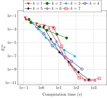
Figure 2: Efficiency of the scheme up to seventh order for the M₃ manufactured solution with optimization tolerance $\tau=10^{-11}$.

5.2 Plane source

In this test case we start with an isotropic distribution where the initial mass is concentrated in the middle of an infinite domain $x\in(-\infty,\infty)$:

$$\psi_{t=0}(x,\mu)=\psi_{\rm floor}+\delta(x)$$

where the small parameter $\psi_{\rm floor}=0.5\times 10^{-8}$ is used to approximate a vacuum. In practice, a bounded domain must be used, so we choose a domain large enough that the boundary should have only negligible effects on the solution: thus for our final time $t_{\rm f}=1$, we take $X=[x_{\text{L}},x_{\text{R}}]=[-1.2,1.2]$. At the boundary we set

$$\psi_{\text{L}}(t,\mu)\equiv\psi_{\rm floor}\quad\mbox{and}\quad\psi_{\text{R}}(t,\mu)\equiv\psi_{\rm floor}$$

We set $\sigma_{\mathrm{s}}=1$ and $\sigma_{\mathrm{a}}=0$.

All solutions here are computed with an even number of cells, so the delta function in the initial condition lies on a cell boundary. Therefore we approximate the delta function by splitting it into the cells immediately to the left and right.

Since this is a highly non-smooth problem, the choice of $c$ is not immediately obvious. Indeed, the solution contains such strong gradients, so choosing $c$ too small can greatly reduce the accuracy of the simulation. After some numerical experimentation, we observed that in the $1000$-cell seventh-order simulations the value $c=15$ generally gave a good trade-off between smoothness in the solution without adding too much diffusivity. In the $4000$-cell fourth-order simulations, where the non-smoothness is further resolved, $c=10$ gave the best results.

In Figure 3 and Figure 4, we plot several solutions at the final time for the M₃ and M₇ models, respectively, as well as a reference solution of the kinetic equation (2.1). We consider numerical solutions of orders $k\in\{1,4,7\}$. The first-order solutions are included to indicate our best guess of the true $\text{M}_{N}$ solutions, and they largely agree with those presented in [18] (although we have computed solutions on a much finer grid in order to better resolve sharp peaks in the solutions).

In Figure 3, we present seventh-order M₃ solutions. In Figure LABEL:fig:plane-M3-PP, we see that while the seventh-order solution using only the positivity-preserving limiter closely matches the highly-resolved first-order solution, some spurious oscillations around $x=\pm 0.25$ remain. These oscillations are largely removed by using the maximum-principle limiter with $c=15$, as we see in Figure LABEL:fig:plane-M3-PP-vs-MP-mid, though in Figure LABEL:fig:plane-M3-PP-vs-MP-front we see that this solution is also somewhat more diffusive.

The M₇ solution to the plane-source problem is more oscillatory. Figure LABEL:fig:plane-M7-k4 shows that our kinetic scheme with fourth-order reconstructions and the maximum-principle limiter performs well. However, seventh-order solutions are notably more diffusive, as shown at the leading edge of the solution in Figure LABEL:fig:plane-M7-k7.

That the high-order solutions are more diffusive than the true $\text{M}_{N}$ solutions is not necessarily a disadvantage: the more diffusive solutions are actually closer to the reference kinetic solution. Indeed, the $\text{M}_{N}$ equations are a spectral method for the original kinetic equation, and thus should not be applied to a non-smooth problem like this one without filtering to avoid the Gibbs phenomenon. Exactly how to apply such a filter for moment models kinetic equations is a topic of ongoing research [26, 30], but here it seems that the maximum-principle limiter already filters the solution somewhat.

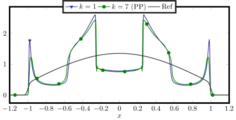
(a) M₃ with the positivity-preserving limiter

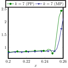
(b) M₃, $c=15$

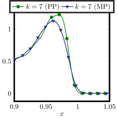
(c) M₃, $c=15$

Figure 3: The local particle density $u_{0}$ from first- and seventh-order solutions to the plane-source problem with the M₃ $t=1$. First-order solutions were computed with ${J}=10000$ cells and seventh-order with ${J}=1000$ cells.

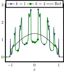
(a) M₇, $k=4$, $c=10$

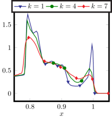
(b) M₇, $k=7$, $c=15$

Figure 4: The local particle density $u_{0}$ from first-, fourth- and seventh-order solutions to the plane-source problem with the M₇ model at $t=1$. First-order solutions were computed with ${J}=10^{4}$ cells; fourth-order with ${J}=4000$ cells; and seventh-order with ${J}=1000$ cells.

5.3 Source-beam

Finally we present a discontinuous version of the source-beam problem from [14]. The spatial domain is $X=[0,3]$, and

$$\sigma_{\mathrm{a}}(x)=\begin{cases}1&\text{ if }x\leq 2\\ 0&\text{ else}\end{cases},\quad\sigma_{\mathrm{s}}(x)=\begin{cases}0&\text{ if }x\leq 1\\ 2&\text{ if }1<x\leq 2\\ 10&\text{ else}\end{cases},\quad S(x)=\begin{cases}1&\text{ if }1\leq x\leq 1.5\\ 0&\text{ else}\end{cases},$$

with initial and boundary conditions

$$\psi_{t=0}(x,\mu)\equiv\psi_{\rm floor},$$

$$\psi_{\text{L}}(t,\mu)=\beta\exp(-\gamma(\mu-1)^{2})\quad\mbox{and}\quad\psi_{\text{R}}(t,\mu)\equiv\psi_{\rm floor},$$

for $\gamma=10^{5}$, normalization constant $\beta=\langle\exp(-\gamma(\mu-1)^{2})\rangle^{-1}$, and $\psi_{\rm floor}=0.5\times 10^{-10}$.

$\text{M}_{N}$ solutions for this problem are shown in Figure 5a using ${J}=150$ cells and seventh-order reconstructions, using the maximum-principle limiter with $c=1$, along with a reference solution. We see that increasing the moment order to $N=3$ qualitatively improves the solution significantly.

Figure 5b shows some strengths and weaknesses of our scheme for the M₁ model, where for this problem the shock is the strongest. When compared to a much more finely resolved low-order approximation, the seventh-order approximation on a coarse grid nicely fits the features of the solution despite the discontinuous physical parameters. However, the incoming beam can only be resolved up to first order (note the piecewise-constant approximations behind the beam), resulting in a more diffusive solution at the shock around $x=1$.

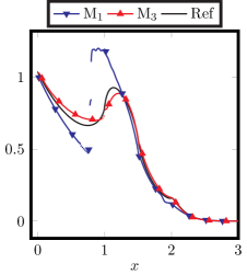
(a) Seventh-order $\text{M}_{N}$ solutions, ${J}=150$

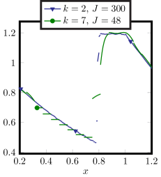
(b) Order comparison for M₁

Figure 5: Seventh-order approximation of several $\text{M}_{N}$ solutions for the source-beam testcase and comparison of the seventh-order approximation on a coarse grid with the second-order approximation on a finer grid.

The source-beam problem is particularly well-suited to test the oscillation-dampening effects of the limiters. In Figure 6 we compare several seventh-order solutions. First in Figure 6a we see in the M₁ solution that the positivity-preserving limiter does not dampen spurious oscillations while the maximum principle-preserving limiter does a better job even for a relatively large value of $c$. Second, in Figure 6b, we show with the M₂ model that for small values of $c$, the maximum principle-preserving limiter is too diffusive.

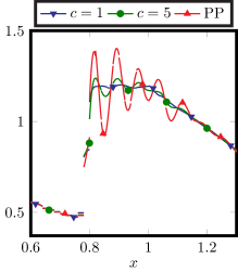
(a) A closer look at oscillations in the M₁ solution for different limiter configurations.

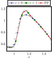
(b) Examining the diffusivity in the M₂ model for different limiter configurations.

Figure 6: The effects of different limiting in the source-beam test at $t=2.5$ for seventh-order solutions with ${J}=150$ cells.

6 Conclusions and outlook

In this paper we describe how to implement a kinetic scheme of (in principle) arbitrarily high order for entropy-based moment closures of linear kinetic equations in one space dimension. For spatial reconstructions we use the well-known WENO method to reconstruct the underlying entropy ansätze using interpolating polynomials, and time integration is performed using multi-step SSP methods. These SSP time integrators play a key role in allowing us to give a time-step restriction which guarantees that the moments stay in the realizable set. The other key component is a limiter, which not only ensures positivity of the polynomial reconstructions on a spatial quadrature set, but also enforces a local maximum principle which dampens spurious oscillations in numerical solutions.

We performed convergence tests with a manufactured solution that included the effects of a space- and time-dependent absorption interaction coefficient, and these results validated that the scheme is converging at least as fast as expected, and often faster at lower resolutions with higher orders. The convergence tests also showed that errors from the numerical optimization routine needed for the angular reconstructions limit the overall accuracy of the scheme. This indeed eliminates the benefit of going beyond a certain order (depending on the optimization tolerance $\tau$). However, our manufactured-solution tests showed that increases in efficiency can be obtained before the optimization errors dominate the solution.

Using the plane-source, an challenging highly non-smooth benchmark problem, we showed that with the maximum-principle limiter accurate solutions can be obtained which even limit some of the spurious oscillations due to Gibbs phenomena in the true $\text{M}_{N}$ solutions, thus pushing our solutions closer to the kinetic solution. However, the choice of the parameter $c$ plays an important role in the approximation quality of the scheme, and a good value is not always available a priori. With another benchmark problem, the source beam, we also demonstrated the benefit of using the maximum principle-preserving limiter. Again, one must strike a balance between flattening smooth extrema and dampening spurious oscillations with the choice of its parameter.

Compared to the discontinuous-Galerkin implementation in [4], where realizability preservation is complex due to the structure of the set of realizable moments, realizability preservation on the kinetic level is much simpler. However, the wider stencils in the WENO reconstruction process will influence the overall parallelizability of the scheme.

Future work should continue to work toward practical implementations of entropy-based moment closures. Models in two and three spatial dimensions should be implemented, and here a notable challenge is the increasing number of angular quadrature points that will be needed. Indeed, our reconstructions are performed at every angular quadrature point, so more efficient WENO techniques will be necessary. Other collision models should also be considered. The Laplace-Beltrami operator in the Fokker-Planck equation does not fall under the types of collision operators considered here but is an important model for problems with forward-peaked scattering. This appears, for example, in important applications such as radiotherapy. Finally, since we have only considered explicit time-stepping schemes, our time-step restriction scales with the mean-free path. Implicit-explicit or asymptotic-preserving schemes should be developed to handle moment models near diffusive or fluid regimes without requiring extremely small time steps.

References

- [1] http://www.mathematik.uni-kl.de/techno/research/high-order/weno/.
- [2] G. Alldredge, C. Hauck, and A. Tits. High-Order Entropy-Based Closures for Linear Transport in Slab Geometry II: A Computational Study of the Optimization Problem. SIAM Journal on Scientific Computing, 34(4):B361–B391, 2012.
- [3] G. W. Alldredge, C. D. Hauck, D. P. O’Leary, and A. L. Tits. Adaptive change of basis in entropy-based moment closures for linear kinetic equations. Journal of Computational Physics, pages 489–508, 2014.
- [4] Graham Alldredge and Florian Schneider. A realizability-preserving discontinuous Galerkin scheme for entropy-based moment closures for linear kinetic equations in one space dimension. Journal of Computational Physics, 295:665–684, August 2015.
- [5] C. Bresten, S. Gottlieb, Z. Grant, D. Higgs, D. I. Ketcheson, and A. Németh. Strong Stability Preserving Multistep Runge-Kutta Methods. July 2013.
- [6] T. A. Brunner. Forms of approximate radiation transport. Tech. Rep SAND2002-1778, 2002.
- [7] Jun-Bo Cheng, Eleuterio F Toro, Song Jiang, and Weijun Tang. A sub-cell weno reconstruction method for spatial derivatives in the ader scheme. Journal of Computational Physics, 251:53–80, 2013.
- [8] B. Cockburn and C.-W. Shu. TVB Runge-Kutta local projection discontinuous Galerkin finite element method for conservation laws II: General framework. Math. Comp., 52(186):411–435, 1989.
- [9] R. Curto and L. Fialkow. Recursiveness, positivity and truncated moment problems. Houston J. Math, 17(4):603–635, 1991.
- [10] B. Dubroca and J. L. Feugeas. Entropic moment closure hierarchy for the radiative transfer equation. C. R. Acad. Sci. Paris Ser. I, 329:915–920, 1999.
- [11] B. Dubroca, M. Frank, A. Klar, and G. Thömmes. Half space moment approximation to the radiative heat transfer equations. ZAMM, 83:853–858, 2003.
- [12] B. Dubroca and A. Klar. Half moment closure for radiative transfer equations. J. Comput. Phys., 180:584–596, 2002.
- [13] M. Frank, H. Hensel, and A. Klar. A fast and accurate moment method for the fokker–planck equation and applications to electron radiotherapy. SIAM Journal on Applied Mathematics, 67(2):582–603, 2007.
- [14] Martin Frank, Cory D Hauck, and Edgar Olbrant. Perturbed, entropy-based closure for radiative transfer. Kinetic and Related Models, 6(3):557–587, 2013.
- [15] C. K. Garrett and C. D. Hauck. A Comparison of Moment Closures for Linear Kinetic Transport Equations: The Line Source Benchmark. Transport Theory and Statistical Physics, 42(6–7):203–235, 2013.
- [16] E. M. Gelbard. Simplified spherical harmonics equations and their use in shielding problems. Technical Report WAPD-T-1182, Bettis Atomic Power Laboratory, 1961.
- [17] S. Gottlieb. On High Order Strong Stability Preserving Runge-Kutta and Multi Step Time Discretizations. Journal of Scientific Computing, 25(1):105–128, October 2005.
- [18] C. Hauck. High-order entropy-based closures for linear transport in slab geometry. Commun. Math. Sci., 9:187–205, 2011.
- [19] M. Junk. Maximum entropy for reduced moment problems. Math. Meth. Mod. Appl. Sci., 10:1001–1025, 2000.
- [20] D. Ketcheson, S. Gottlieb, and C. Macdonald. Strong stability preserving two-step Runge-Kutta methods. SIAM Journal on Numerical Analysis, 49(6):2618–2639, 2011.
- [21] C. K. S. Lam and C. P. T. Groth. Numerical prediction of three-dimensional non-equilibrium flows using the regularized gaussian moment closure. In Proc. of the 20th AIAA Computational Fluid Dynamics Conference, number 3401, 2011.
- [22] E. W. Larsen and C. G. Pomraning. The theory as an asymptotic limit of transport theory in planar geometry—I: Analysis. Nucl. Sci. Eng, 109:49–75, 1991.
- [23] E. W. Larsen and C. G. Pomraning. The theory as an asymptotic limit of transport theory in planar geometry—II: Numerical results. Nucl. Sci. Eng., 109:76–85, 1991.
- [24] C. D. Levermore. Moment closure hierarchies for kinetic theories. J. Stat. Phys., 83:1021–1065, 1996.
- [25] E. E. Lewis and W. F. Miller, Jr. Computational Methods in Neutron Transport. John Wiley and Sons, New York, 1984.
- [26] Ryan G. McClarren and Cory D. Hauck. Robust and accurate filtered spherical harmonics expansions for radiative transfer. Journal of Computational Physics, 229(16):5597 – 5614, 2010.
- [27] J. G. McDonald and C. P. T. Groth. Towards realizable hyperbolic moment closures for viscous heat-conducting gas flows based on a maximum-entropy distribution. Continuum Mechanics and Thermodynamics, 25(5):573–603, 2013.
- [28] E. Olbrant, C. D. Hauck, and M. Frank. A realizability-preserving discontinuous Galerkin method for the M1 model of radiative transfer. Journal of Computational Physics, 231(17):5612–5639, July 2012.
- [29] G. C. Pomraning. Variational boundary conditions for the spherical harmonics approximation to the neutron transport equation. Ann. Phys., 27:193–215, 1964.
- [30] David Radice, Ernazar Abdikamalov, Luciano Rezzolla, and Christian D. Ott. A new spherical harmonics scheme for multi-dimensional radiation transport i. static matter configurations. Journal of Computational Physics, 242(0):648 – 669, 2013.
- [31] S. J. Ruuth and R. J. Spiteri. High-Order Strong-Stability-Preserving Runge–Kutta Methods with Downwind-Biased Spatial Discretizations. SIAM Journal on Numerical Analysis, 42(3):974–996, January 2004.
- [32] F. Schneider, G. Alldredge, M. Frank, and A. Klar. Higher Order Mixed-Moment Approximations for the Fokker–Planck Equation in One Space Dimension. SIAM Journal on Applied Mathematics, 74(4):1087–1114, 2014.
- [33] J. A. Shohat and J. D. Tamarkin. The Problem of Moments. American Mathematical Society, New York, 1943.
- [34] CW Shu. Essentially non-oscillatory and weighted essentially non-oscillatory schemes for hyperbolic conservation laws. 1998.
- [35] H. Struchtrup. Kinetic schemes and boundary conditions for moment equations. Z. Angew. Math. Phys., 51(3):346–365, 2000.
- [36] E.F. Toro. Riemann Solvers and Numerical Methods for Fluid Dynamics: A Practical Introduction. Springer, 2009.
- [37] X. Zhang. Maximum-principle-satisfying and positivity-preserving high order schemes for conservation laws. PhD thesis, Brown University, 2011.
- [38] X. Zhang and C.-W. Shu. On maximum-principle-satisfying high order schemes for scalar conservation laws. Journal of Computational Physics, 229(9):3091–3120, 2010.
- [39] X. Zhang and C.-W. Shu. On positivity-preserving high order discontinuous Galerkin schemes for compressible Euler equations on rectangular meshes. Journal of Computational Physics, 229(23):8918–8934, 2010.
- [40] X. Zhang, Y. Xia, and C.-W. Shu. Maximum-Principle-Satisfying and Positivity-Preserving High Order Discontinuous Galerkin Schemes for Conservation Laws on Triangular Meshes. Journal of Scientific Computing, 50(1):29–62, 2012.
- [41] Xiangxiong Zhang and Chi Wang Shu. A minimum entropy principle of high order schemes for gas dynamics equations. Numerische Mathematik, 121(3):545–563, 2012.