Universal electric current of interacting resonant-level models with asymmetric interactions: An extension of the Landauer formula

Abstract

We study the electron transport in open quantum-dot systems described by the interacting resonant-level models with Coulomb interactions. We consider the situation in which the quantum dot is connected to the left and right leads asymmetrically. We exactly construct many-electron scattering eigenstates for the two-lead system, where two-body bound states appear as a consequence of one-body resonances and the Coulomb interactions. By using an extension of the Landauer formula, we calculate the average electric current for the system under bias voltages in the first order of the interaction parameters. Through a renormalization-group technique, we arrive at the universal electric current, where we observe the suppression of the electric current for large bias voltages, i.e., negative differential conductance. We find that the suppressed electric current is restored by the asymmetry of the system parameters.

I Introduction

In the last two decades, much progress has been made in the experimental studies of the electron transport in nanoscale devices D. Goldhaber-Gordon, Hadas Shtrikman, D. Mahalu, David Abusch-Magder, U. Meirav, and M. A. Kastner (1998); Cronenwett et al. (1998); W. G. van der Wiel, S. De Franceschi, T. Fujisawa, J. M. Elzerman, S. Tarucha, and L. P. Kouwenhoven (2000); Andrey V. Kretinin, Hadas Shtrikman, David Goldhaber-Gordon, Markus Hanl, Andreas Weichselbaum, Jan von Delft, Theo Costi, and Diana Mahalu (2011). In the systems smaller than the coherent length, quantum effects are observed in the electron transport A. Yacoby, M. Heiblum, D. Mahalu, and Hadas Shtrikman (1995); R. Schuster, E. Buks, M. Heiblum, D. Mahalu, V. Umansky, and Hadas Shtrikman (1997). In order to analyze it beyond the linear-response regime theoretically, we need to treat nonequilibrium steady states realized in open quantum systems. The Landauer formula Datta (1995); Imry (2002) enables the calculation of the electric current flowing across nanoscale samples in noninteracting cases, which indicates that the nonequilibrium steady states are scattering states in the open quantum systems. Indeed, the transport properties such as the electrical conductance and the electric-current noise are determined by the scattering matrix Yurke and Kochanski (1990); M. Büttiker (1992); Blanter and M. Büttiker (2000). To investigate interacting cases, the Keldysh formalism of the nonequilibrium Green’s function has been developed C. Caroli, R. Combescot, P. Nozieres, and D. Saint-James (1971); Meir et al. (1991); Meir and Wingreen (1992); Hershfield et al. (1992); Haug and Jauho (2007). It has provided a standard tool for the study of the Kondo effect measured as a conductance peak in semiconductor quantum dots (QDs) Ng and Lee (1988); Wingreen and Meir (1994). On the other hand, we have proposed an extension of the Landauer formula to interacting cases Nishino et al. (2009, 2011), and have shown that the scattering states are essential in the interacting cases as well.

The interacting resonant-level model (IRLM) is one of the standard testbeds for such studies of the open QD systems with interactions. The original IRLM, which consists of a single impurity coupled to a conduction band, was introduced for studying the Kondo problem in equilibrium systems Filyov and Wiegmann (1980). Recently, the IRLM with two external leads has been employed as a minimal model of open QD systems with Coulomb interactions; it plays an important role in verifying the theoretical approaches such as the nonequilibrium Bethe-ansatz approach Mehta and Andrei (2006), the perturbation theory with the numerical renormalization group Borda et al. (2007), a new method called impurity conditions Doyon (2007) and the time-dependent density-matrix renormalization-group method Boulat et al. (2008).

A remarkable feature of the two-lead IRLM is the appearance of negative differential conductance, that is, the suppression of the electric current due to the Coulomb interaction for large bias voltages. Clearly, this is a phenomenon out of the linear-response regime. To see the feature and to compare the results obtained by different approaches, the universal electric current characterized by a single scaling parameter $T_{\rm K}$ is useful Doyon (2007); Doyon and Andrei (2006); Golub (2007). Indeed, it is found that, for large bias voltages $V$, the universal electric current shows a power-law decay $\langle I\rangle\propto(V/T_{\rm K})^{-U/\pi}$ with the parameter $U$ of the Coulomb interaction Doyon (2007); Boulat et al. (2008).

In the previous papers Nishino et al. (2009, 2011), we proposed an extension of the Landauer formula with many-electron scattering eigenstates. We considered the two-lead IRLM with linearized dispersion relations and gave exact many-electron scattering eigenstates in explicit forms. This is in contrast to the previous studies Aharony et al. (2000); Goorden and M. Büttiker (2007); Lebedev et al. (2008) of the scattering problems for other QD systems, which include integrals or matrix inversions. The explicit $N$-electron scattering eigenstates enabled us to calculate the quantum-mechanical expectation value of the electric current, which we called the $N$-electron current. By taking the electron-reservoir limit $N\to\infty$ of the $N$-electron current, we obtained the average electric current for the system under finite bias voltages. It is clear that the way of realizing the nonequilibrium steady states in our extension of the Landauer formula is different from the Keldysh formalism C. Caroli, R. Combescot, P. Nozieres, and D. Saint-James (1971); Meir et al. (1991); Meir and Wingreen (1992); Hershfield et al. (1992); Haug and Jauho (2007). By employing a renormalization-group technique with the Callan-Symanzik equation Doyon (2007); Golub (2007), we arrived at the universal electric current in the first order of the interaction parameter $U$. We found that the negative differential conductance of the universal electric current is characterized by the same scaling parameter $T_{\rm K}$ as that obtained by other approaches Doyon (2007); Golub (2007); C. Karrasch, S. Andergassen, M. Pletyukhov, D. Schuricht, L. Borda, V. Meden, and H. Schoeller (2010). We remark that the apparent inconsistency in Ref. Nishino et al., 2009 pointed out in Ref. S. Andergassen, M. Pletyukhov, D. Schuricht, H. Schoeller, and L. Borda, 2011 is removed in the level of the universal electric current Schuricht .

In the present paper, we study the two-lead IRLM in which the QD is connected to the two external leads asymmetrically. The effect of the asymmetry of the QD systems is observed in experiments. For example, in semiconductor QDs W. G. van der Wiel, S. De Franceschi, T. Fujisawa, J. M. Elzerman, S. Tarucha, and L. P. Kouwenhoven (2000); Andrey V. Kretinin, Hadas Shtrikman, David Goldhaber-Gordon, Markus Hanl, Andreas Weichselbaum, Jan von Delft, Theo Costi, and Diana Mahalu (2011), the asymmetry of the lead-dot couplings causes breaking of the unitary limit of the Kondo effect, which is theoretically understood in the linear-response regime Ng and Lee (1988); Wingreen and Meir (1994). In the present study, we investigate the effect of the asymmetry on electron transport out of the linear-response regime. One of the theoretical difficulties of the asymmetric cases is that the even-odd transformation, which maps the two-lead IRLM to two single-lead systems Mehta and Andrei (2006); Nishino et al. (2009, 2011), does not work. The application of the Bethe-ansatz approach Mehta and Andrei (2006) has been restricted to the cases in which the even-odd transformation works. The construction of exact many-electron scattering eigenstates for such pure two-lead systems is established for the first time in this paper.

Through the extension of the Landauer formula and a renormalization-group technique, we obtain the universal electric current for the asymmetric cases in the first order of the Coulomb-interaction parameters $U_{1}$ and $U_{2}$. The universal electric current is characterized by the two renormalized parameters $T_{1}$ and $T_{2}$. The sum $T_{\rm K}=T_{1}+T_{2}$ provides a scaling parameter for the bias voltage $V$, which is similar to the symmetric cases. Our universal electric current has the same functional form as that obtained by the renormalization-group approach C. Karrasch, S. Andergassen, M. Pletyukhov, D. Schuricht, L. Borda, V. Meden, and H. Schoeller (2010); S. Andergassen, M. Pletyukhov, D. Schuricht, H. Schoeller, and L. Borda (2011), although there is a difference in our calculation of the renormalized parameters $T_{1}$ and $T_{2}$. As we will point at the end of Section IV, this leads to a critical difference in the predicted behavior of the universal electric current. The suppressed electric current due to the Coulomb interaction is restored by the asymmetry of the system parameters. To clarify the relation between the asymmetry of the system parameters and the restoration of the suppressed electric current, we introduce the asymmetry parameter $\delta=(U_{1}-U_{2})(T_{1}-T_{2})/(2T_{\rm K})$ taking the value in the range $0\leq\delta<\bar{U}$ with the average interaction $\bar{U}=(U_{1}+U_{2})/2$. In fact, in the first order of $U_{1}$ and $U_{2}$, the power-law decay of the universal electric current is given by $\langle I\rangle\propto(V/T_{\rm K})^{-(\bar{U}-\delta)/\pi}$, which indicates that the restoration of the suppressed electric current occurs with both asymmetric Coulomb interactions and asymmetric lead-dot couplings. The restoration was reported to happen even for symmetric lead-dot couplings in Refs. C. Karrasch, S. Andergassen, M. Pletyukhov, D. Schuricht, L. Borda, V. Meden, and H. Schoeller, 2010 and S. Andergassen, M. Pletyukhov, D. Schuricht, H. Schoeller, and L. Borda, 2011, but we presume that this was due to higher orders of the interaction $U_{\ell}$ in the renormalized parameters $T_{1}$ and $T_{2}$.

The exact many-electron scattering eigenstates tell us much about the transport properties of interacting electrons in the open QD systems. We notice that the scattering processes in which the set of wave numbers of incident plane waves is not conserved are essential in interacting cases. The explicit form of the scattering eigenstates indicates that, due to the Coulomb interactions, the incident plane-wave states are partially scattered to many-body bound states that decay exponentially as the electrons separate from each other. Indeed, the two-body bound states appear in the two-lead IRLM; each term of the $N$-electron scattering states is characterized by the configuration of the two-body bound states. We can understand the origin of the negative differential conductance in the two-lead IRLM in terms of the formation of two-body bound states. Such many-body bound states are also found in other open QD systems Imamura et al. (2009); Nishino et al. (2012).

The present paper is organized as follows. In Sec. II.1, we introduce the two-lead IRLM with asymmetric interactions. In Sec. II.2, the extension of the Landauer formula Nishino et al. (2009, 2011) is described in a general setting. In Sec. III, we present the construction of the exact one- and two-electron scattering eigenstates whose incident states are free-electronic plane waves in the leads. We also give the $N$-electron scattering eigenstates in the first order of the Coulomb-interaction parameters. In Sec. IV, through the extension of the Landauer formula, we calculate the average electric current for the system under finite bias voltages. We obtain the universal electric current by dealing with the divergences in the average electric current with the Callan-Symanzik equation. As a result, we observe the negative differential conductance and the restoration of the suppressed electric current. Section V is devoted to concluding remarks.

II Models and formulation

II.1 Interacting resonant-level models

We consider the open QD system described by the IRLM of spinless electrons. It consists of a QD with a single energy level and two external leads of noninteracting electrons. The arrangement of the QD and the two leads is illustrated in Fig. 1. We assume the situation in which the QD is connected to the two leads asymmetrically.

The Hamiltonian is given by

$$H= \sum_{\ell=1,2}\int_{-\frac{L}{2}}^{\frac{L}{2}}dx\,c^{\dagger}_{\ell}(x)\frac{1}{\mathrm{i}}\frac{d}{dx}c_{\ell}(x)+\sum_{\ell=1,2}\big{(}t_{\ell}c^{\dagger}_{\ell}(0)d+t^{\ast}_{\ell}d^{\dagger}c_{\ell}(0)\big{)}+\epsilon_{{\rm d}}d^{\dagger}d$$

$$+\sum_{\ell=1,2}U_{\ell}c^{\dagger}_{\ell}(0)c_{\ell}(0)d^{\dagger}d.$$ (1)

Here $c^{\dagger}_{\ell}(x)$ and $c_{\ell}(x)$ are the creation- and the annihilation-operators of an electron in the lead $\ell$, while $d^{\dagger}$ and $d$ are those on the QD. The first term corresponds to the kinetic energy of electrons in the leads, where $L$ stands for the length of the two leads to be eventually taken to infinity. The second term expresses the tunneling between the leads and the QD, where the parameter $t_{\ell}(\in\mathbb{C})$ is the transfer integral. We assume a single energy level $\epsilon_{\rm d}(\in\mathbb{R})$ on the QD, which corresponds to the third term. The fourth term describes the Coulomb interaction between the two electrons at the origin $x=0$ of the lead $\ell$ and on the QD. The parameter $U_{\ell}(>0)$ is the strength of the Coulomb repulsion.

We focus on the electrons with positive velocities in the vicinity of the Fermi energy $\epsilon_{\mathrm{F}}$ of each lead and linearize the local dispersion relation to be $\epsilon(k)=v_{\mathrm{F}}(k-k_{\mathrm{F}})+\epsilon_{\mathrm{F}}$ under the assumption that the other parameters $|t_{\ell}|$, $|\epsilon_{\rm d}|$ and $U_{\ell}$ are small compared with the Fermi energy $\epsilon_{\mathrm{F}}$ Filyov and Wiegmann (1980). For simplicity, we have set $v_{\mathrm{F}}=1$, $k_{\mathrm{F}}=0$ and $\epsilon_{\mathrm{F}}=0$ in Eq. (II.1). Then, as is indicated in Fig. 1, an electron coming from the part $x<0$ of the lead 1 is scattered at the QD to the parts $x>0$ of the two leads.

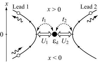
Figure 1: The two-lead interacting resonant-level model. Electrons flow only upward due to the linearized dispersion relations of the leads.

In constructing the scattering eigenstates, we treat the system as an open system in the limit $L\to\infty$ of the two leads. In the sprit of the original Landauer formula Datta (1995); Imry (2002), we suppose that the infinite two leads can substitute for electron reservoirs that are in the Fermi degenerate states of noninteracting electrons. We assume that the electrons emitted from the electron reservoir into the lead $\ell$ follow the Fermi distribution function $f_{\mu_{\ell},\beta_{\ell}}(E)=1/(1+\mathrm{e}^{\beta_{\ell}(E-\mu_{\ell})})$ with the chemical potential $\mu_{\ell}$ and the inverse temperature $\beta_{\ell}$. We are interested in the nonequilibrium steady state realized between the large two electron reservoirs in the cases $\mu_{1}\neq\mu_{2}$ of different chemical potentials.

We adopt a standard definition of the electric-current operator as

$$I=\alpha I_{1}-(1-\alpha)I_{2},\quad I_{\ell}=\mathrm{i}\big{(}t_{\ell}c_{\ell}^{\dagger}(0)d-t^{\ast}_{\ell}d^{\dagger}c_{\ell}(0)\big{)}.\quad(\ell=1,2)$$ (2)

For an arbitrary eigenstate $|\psi\rangle$ of the Hamiltonian $H$, the expectation value $\langle\psi|I|\psi\rangle$ does not depend on the parameter $\alpha$ since the relation $\langle\psi|I_{1}|\psi\rangle=-\langle\psi|I_{2}|\psi\rangle$ holds. In what follows, we choose the parameter $\alpha=|t_{2}|^{2}/t^{2}$ with $t=\sqrt{|t_{1}|^{2}+|t_{2}|^{2}}$ for the convenience of calculations.

II.2 Extension of the Landauer formula

Our purpose is to study the average electric current flowing across the QD of the two-lead IRLM beyond the linear-response regime. The extension of the Landauer formula, which was proposed in Refs. Nishino et al., 2009 and Nishino et al., 2011, consists of the following three steps:

• Construction of many-electron scattering eigenstates whose incident states are free-electronic plane waves in the leads;

• Calculation of the quantum-mechanical expectation value of the electric current with the many-electron scattering eigenstates;

• Calculation of the statistical-mechanical average of the electric current by assuming the equilibration of electrons in each electron reservoir.

The many-electron scattering eigenstates constructed in the step (i) are characterized by the wave numbers of the incident plane waves. We note that they are essentially different from the Bethe-ansatz eigenstates Mehta and Andrei (2006); Filyov and Wiegmann (1980), whose incident states are not free electronic but include the effect of interactions. The Bethe-ansatz result in Ref. Mehta and Andrei, 2006 did not agree with results of the previous works Doyon (2007); Golub (2007); Boulat et al. (2008) while our results agree with them. For the wave numbers $\{k_{1},\ldots,k_{N_{1}}\}$ of the $N_{1}$-electron incident plane wave coming in through the lead 1 and $\{h_{1},\ldots,h_{N_{2}}\}$ of the $N_{2}$-electron incident plane wave coming in through the lead 2, we express the $N$-electron scattering eigenstates by $|k,h\rangle=|k_{1},\ldots,k_{N_{1}},h_{1},\ldots,h_{N_{2}}\rangle$ with $N=N_{1}+N_{2}$. In the step (ii), we calculate the expectation value $\langle k,h|I|k,h\rangle/\langle k,h|k,h\rangle$ of the electric-current operator $I$, which we call the $N$-electron current. This calculation is practically carried out by using the explicit $N$-electron scattering eigenstates. In the step (iii), we take the limit $N_{\ell},L\to\infty$ of the $N$-electron current by assuming that the wave numbers $k_{i}$ and $h_{i}$ of incident plane waves follow the Fermi distribution of each electron reservoir. We call the limit an electron-reservoir limit. Clearly, the reservoir limit corresponds to taking the statistical-mechanical average of the electric current for all the incident states that follow the Fermi distributions. In general, the electrons scattered at the QD are in many-body states including the effect of interactions. We assume that such many-body states are completely equilibrated to the Fermi degenerate state of free electrons in each election reservoir before being re-emitted towards the QD, which is the main assumption of the extension of the Landauer formula. We shall see for the two-lead IRLM that, since the $N$-dependence of the $N$-electron current appears only in the upper bounds of the sums on wave numbers $\{k_{i}\}$ and $\{h_{i}\}$, we can take the reservoir limit by replacing the sums with the integrals on $k$ and $h$ with the Fermi-distribution functions $f_{\mu_{1},\beta}(k)$ and $f_{\mu_{2},\beta}(h)$.

The way of realizing the nonequilibrium steady states in the extension of the Landauer formula is different from that in the Keldysh formalism C. Caroli, R. Combescot, P. Nozieres, and D. Saint-James (1971); Meir et al. (1991); Meir and Wingreen (1992); Hershfield et al. (1992); Haug and Jauho (2007); Golub (2007). In our extension of the Landauer formula, we first construct the $N$-electron scattering eigenstates for finite $N$ without the information of the equilibrium states in the electron reservoirs. After the calculation of the $N$-electron current, we take the reservoir limit to consider the nonequilibrium steady state. In the Keldysh formalism, on the other hand, the Green’s functions or the density operator describing the nonequilibrium steady states are obtained by adiabatically turning on the perturbative terms for the initial nonperturbative steady states of infinite number of electrons.

Our approach is also independent of Hershfield’s bias-operator approach, which constructs the density operator of the nonequilibrium steady states directly from one-electron field operators in the framework of the quantum field theory Hershfield (1993); Han (2006); Anders (2008). We remark that the construction of the density operator through the bias-operator approach has not been established analytically in interacting cases Han (2006); Anders (2008) except for the Toulouse limit of the Kondo model Schiller and Hershfield (1995, 1998).

III Many-electron scattering eigenstates

III.1 One-electron cases

The linearization of the local dispersion relations of the leads enables us to construct exact scattering eigenstates. First, we consider the one-electron cases. The one-electron scattering eigenstates are given in the form

$$|E\rangle =\Big{(}\int\!\!dx\sum_{m=1,2}g_{m}(x)c^{\dagger}_{m}(x)+ed^{\dagger}\Big{)}|0\rangle,$$ (3)

where $|0\rangle$ is the vacuum state satisfying $c_{\ell}(x)|0\rangle=d|0\rangle=0$. The eigenfunctions $g_{m}(x)$ and $e$ are determined by the coupled Schrödinger equations:

$$\Big{(}\frac{1}{\mathrm{i}}\frac{d}{dx}-E\Big{)}g_{m}(x)+t_{m}e\delta(x)=0,\quad(m=1,2)$$

$$(\epsilon_{{\rm d}}-E)e+\sum_{m=1,2}t^{\ast}_{m}g_{m}(0)=0.$$ (4)

It is readily found that the eigenfunction $g_{m}(x)$ is discontinuous at $x=0$ and the matching condition at $x=0$ is obtained by integrating the first equation in Eqs. (III.1) around $x=0$ as

$$g_{m}(0+)-g_{m}(0-)+\mathrm{i}t_{m}e=0.$$ (5)

Since the value $g_{m}(0)$ is not determined by the Schrödinger equations, we assume $g_{m}(0)=(g_{m}(0+)+g_{m}(0-))/2$ from physical intuition.

To employ the Landauer formula, we need the scattering eigenstates whose incident states are a plane wave in the lead 1 or the lead 2. For the incident plane wave with the wave number $k$ in the lead $\ell$, we consider the solution $g^{(\ell)}_{m,k}(x)$ and $e^{(\ell)}_{k}$ of the Schrödinger equations (III.1) satisfying

$$g^{(\ell)}_{m,k}(x)=\frac{1}{\sqrt{2\pi}}\delta_{m\ell}\mathrm{e}^{\mathrm{i}kx}\quad\text{for}\;x<0,$$ (6)

where $\delta_{m\ell}$ is the Kronecker delta. We refer to Eq. (6) as scattering boundary conditions. The solution with energy eigenvalue $E=k$ is given by

$$g^{(\ell)}_{m,k}(x)=\frac{1}{\sqrt{2\pi}}\big{(}\delta_{m\ell}-\mathrm{i}t_{m}\sqrt{2\pi}e^{(\ell)}_{k}\theta(x)\big{)}\mathrm{e}^{\mathrm{i}kx},$$

$$e^{(\ell)}_{k}=\frac{1}{\sqrt{2\pi}}\frac{t_{\ell}^{\ast}}{k-\epsilon_{{\rm d}}+\mathrm{i}\Gamma},$$ (7)

where $\theta(x)$ is the step function and $\Gamma=(|t_{1}|^{2}+|t_{2}|^{2})/2$ is the level width of the QD. By inserting them into Eq. (3), we obtain the scattering eigenstate $|k;\ell\rangle$ whose incident state is a plane wave with wave number $k$ in the lead $\ell$.

The one-electron scattering eigenstates $|k;\ell\rangle$ are normalized on the $\delta$-function as $\langle k;\ell|k^{\prime};\ell^{\prime}\rangle=\delta_{\ell\ell^{\prime}}\delta(k-k^{\prime})$ in the limit $L\to\infty$. In the calculation of quantum-mechanical expectation values of physical quantities with the scattering eigenstates $|k;\ell\rangle$, we need to restore the length $L$ of the leads in order to regularize the square norm as $\langle k;\ell|k;\ell\rangle=L/(2\pi)$.

III.2 Two-electron cases

We next consider the two-electron cases as the simplest example of the interacting cases. The form of the two-electron scattering eigenstates is given by

$$|E\rangle =\Big{(}\sum_{l,m=1,2}\int_{x_{1}<x_{2}}dx_{1}dx_{2}\,g_{lm}(x_{1},x_{2})c^{\dagger}_{l}(x_{1})c^{\dagger}_{m}(x_{2})+\sum_{l=1,2}\int\!dx\,e_{l}(x)c^{\dagger}_{l}(x)d^{\dagger}\Big{)}|0\rangle.$$ (8)

Here we impose the antisymmetric relation $g_{lm}(x_{1},x_{2})=-g_{ml}(x_{2},x_{1})$. The eigenvalue problem $H|E\rangle=E|E\rangle$ leads to the coupled Schrödinger equations:

$$\Big{(}\frac{1}{\mathrm{i}}\Big{(}\frac{\partial}{\partial x_{1}}+\frac{\partial}{\partial x_{2}}\Big{)}-E\Big{)}g_{lm}(x_{1},x_{2})+t_{m}e_{l}(x_{1})\delta(x_{2})-t_{l}\delta(x_{1})e_{m}(x_{2})=0,$$ (9a)

$$\Big{(}\frac{1}{\mathrm{i}}\frac{d}{dx}+\epsilon_{{\rm d}}+U_{l}\delta(x)-E\Big{)}e_{l}(x)+\sum_{m=1,2}t^{\ast}_{m}g_{lm}(x,0)=0.$$ (9b)

In the previous works Nishino et al. (2009, 2011) for the symmetric case $U_{1}=U_{2}$, we employed the even-odd transformation that maps the two-lead IRLM to two single-lead systems. However, since the transformation does not work for the asymmetric cases $U_{1}\neq U_{2}$, we deal with the two-lead IRLM directly.

We present a construction of the exact two-electron scattering eigenstates, which is an extension of the previous one Shen and Fan (2007); Nishino et al. (2009, 2011). First, we derive three important relations from the Schrödinger equations (9a) and (9b). The eigenfunction $g_{lm}(x_{1},x_{2})$ is discontinuous at $x_{1}=0$ and $x_{2}=0$, while $e_{l}(x)$ is discontinuous at $x=0$. The matching conditions at the discontinuous points are given by

$$g_{lm}(x,0+)-g_{lm}(x,0-)+\mathrm{i}t_{m}e_{l}(x)=0,$$ (10a)

$$e_{l}(0+)-e_{l}(0-)+\mathrm{i}U_{l}e_{l}(0)=0,$$ (10b)

which are obtained by integrating the Schrödinger equations (9a) and (9b) around the discontinuous points. Since the values of the eigenfunctions at the discontinuous points are not determined by the Schrödinger equations, we assume

$$g_{lm}(x,0)=\frac{1}{2}\big{(}g_{lm}(x,0+)+g_{lm}(x,0-)\big{)},$$ (11a)

$$e_{l}(0)=\frac{1}{2}\big{(}e_{l}(0+)+e_{l}(0-)\big{)}$$ (11b)

in a way similar to the one-electron cases. By applying Eqs. (10a) and (11a) to Eq. (9b) for $x\neq 0$, we have

$$\Big{(}\frac{1}{\mathrm{i}}\frac{d}{dx}+\epsilon_{\rm d}-\mathrm{i}\Gamma-E\Big{)}e_{l}(x)=-\sum_{m}t_{m}^{\ast}g_{lm}(x,0-).$$ (12)

Given functions $g_{lm}(x,0-)$, $(m=1,2)$, we obtain the general solution for $e_{l}(x)$ as

$$e_{l}(x) =C_{l}\mathrm{e}^{\mathrm{i}(E-\epsilon_{\rm d}+\mathrm{i}\Gamma)x}-\mathrm{i}\sum_{m}t_{m}^{\ast}\int_{x_{0}}^{x}dz\,\mathrm{e}^{\mathrm{i}(E-\epsilon_{\rm d}+\mathrm{i}\Gamma)(x-z)}g_{lm}(z,0-),$$ (13)

where $C_{l}$ is the integration constant and $x_{0}$ is chosen as $x_{0}=-\infty$ if $x<0$ and $x_{0}=0$ otherwise. On the other hand, by applying Eq. (11b) to Eq. (10b), we have the matching condition

$$\Big{(}1+\frac{\mathrm{i}}{2}U_{l}\Big{)}e_{l}(0+)=\Big{(}1-\frac{\mathrm{i}}{2}U_{l}\Big{)}e_{l}(0-).$$ (14)

The equations (10a), (13) and (14) are the relations that we need.

$(\ell_{1},\ell_{2})$	$A_{11,(12)}$	$A_{11,(21)}$	$A_{12,(12)}$	$A_{12,(21)}$	$A_{22,(12)}$	$A_{22,(21)}$
$(1,1)$	$1$	$-1$	$0$	$0$	$0$	$0$
$(1,2)$	$0$	$0$	$1$	$0$	$0$	$0$
$(2,2)$	$0$	$0$	$0$	$0$	$1$	$-1$

Table 1: The coefficients $A_{\ell m,P}$ of the incident plane-wave states for $(\ell_{1},\ell_{2})=(1,1),(1,2)$ and $(2,2)$.

Next, we demonstrate how to construct the two-electron scattering eigenstates by the repeated use of the three equations (10a), (13) and (14). Let us consider the situation in which one electron with wave number $k_{1}$ is coming in through the lead $\ell_{1}$ and another with $k_{2}$ is coming in through the lead $\ell_{2}$. We construct the eigenfunctions with energy eigenvalue $E=k_{1}+k_{2}$ that satisfy the scattering boundary conditions

$$g_{lm}(x_{1},x_{2}) =\frac{1}{2\pi}\sum_{P}A_{lm,P}\mathrm{e}^{\mathrm{i}(k_{P_{1}}x_{1}+k_{P_{2}}x_{2})}$$ (15)

for $x_{1},x_{2}<0$. Here $P=(P_{1},P_{2})$ is a permutation of $(1,2)$ and the coefficients $A_{lm,P}$ are given by $A_{lm,P}=\mathrm{sgn}(P)\delta_{l\ell_{P_{1}}}\delta_{m\ell_{P_{2}}}$ with the signature $\mathrm{sgn}(P)$ of the permutation $P$. The coefficients $A_{lm,P}$ are explicitly listed on Table 1. Beginning from the incident state $g_{\ell m}(x_{1},x_{2})$ in the region $x_{1}<x_{2}<0$, we connect it to the other regions through Eqs. (10a), (13) and (14). By inserting $g_{lm}(x,0-)$ into Eq. (13), we have

$$e_{l}(x) =\frac{1}{\sqrt{2\pi}}\sum_{P,m}A_{lm,P}e^{(m)}_{k_{P_{2}}}\mathrm{e}^{\mathrm{i}k_{P_{1}}x}$$ (16)

for $x<0$. Here we have set $x_{0}=-\infty$ and have taken $C_{l}=0$ to avoid the divergence as $x\to-\infty$. The function $g_{lm}(x,0-)$ is connected to $g_{lm}(x,0+)$ by Eq. (10a) with Eq. (16) as

$$g_{lm}(x,0+)=\frac{1}{2\pi}\sum_{P,n}A_{ln,P}\mathrm{e}^{\mathrm{i}k_{P_{1}}x}(\delta_{mn}-\mathrm{i}t_{m}\sqrt{2\pi}e^{(n)}_{k_{P_{2}}}),$$ (17)

which leads to

$$g_{lm}(x_{1},x_{2})=\frac{1}{\sqrt{2\pi}}\sum_{P,n}A_{ln,P}\mathrm{e}^{\mathrm{i}k_{P_{1}}x_{1}}g_{m,k_{P_{2}}}^{(n)}(x_{2})$$ (18)

for $x_{1}<0<x_{2}$. Recall that $g_{m,k}^{(n)}(x)$ is the one-electron scattering eigenfunction in Eqs. (III.1). Again, by inserting $g_{lm}(x,0-)$ into Eq. (13), we have

$$e_{l}(x) =C^{\prime}_{l}\mathrm{e}^{\mathrm{i}(E-\epsilon_{\rm d}+\mathrm{i}\Gamma)x}-\sum_{P,m,n}A_{mn,P}g_{l,k_{P_{2}}}^{(n)}(x)e_{k_{P_{1}}}^{(m)}$$ (19)

for $x>0$. Here we keep the first term with the integration constant $C^{\prime}_{l}$ since the term is not divergent as $x\to\infty$. By inserting $g_{lm}(0-,x)$ and $e_{l}(x)$, $(x>0)$ into Eq. (10a) with the antisymmetric relation $g_{lm}(x_{1},x_{2})=-g_{ml}(x_{2},x_{1})$, we have

$$g_{lm}(x_{1},x_{2}) =\sum_{P,r,n}A_{rn,P}g_{l,k_{P_{1}}}^{(r)}(x_{1})g_{m,k_{P_{2}}}^{(n)}(x_{2})+\mathrm{i}t_{l}C^{\prime}_{m}\mathrm{e}^{\mathrm{i}((\epsilon_{\rm d}-\mathrm{i}\Gamma)x_{1}+(E-\epsilon_{\rm d}+\mathrm{i}\Gamma)x_{2})}$$ (20)

for $0<x_{1}<x_{2}$. Finally, by inserting Eqs. (16) and (19) into Eq. (14), we determine the integration constant $C_{l}^{\prime}$ as

$$C^{\prime}_{l}=\frac{1}{\sqrt{2\pi}}\mathrm{i}u_{l}\big{(}\delta_{l\ell_{2}}e^{(\ell_{1})}_{k_{1}}-\delta_{l\ell_{1}}e^{(\ell_{2})}_{k_{2}}\big{)}$$ (21)

with $u_{l}=2U_{l}/(2+\mathrm{i}U_{l})$. Thus the two-electron scattering eigenfunctions satisfying the scattering boundary conditions (15) are obtained as follows:

$$g^{(\ell_{1}\ell_{2})}_{lm,k_{1}k_{2}}(x_{1},x_{2}) =g^{(\ell_{1})}_{l,k_{1}}(x_{1})g^{(\ell_{2})}_{m,k_{2}}(x_{2})-g^{(\ell_{2})}_{l,k_{2}}(x_{1})g^{(\ell_{1})}_{m,k_{1}}(x_{2})$$

$$\quad+t_{l}u_{m}Z^{(\ell_{1}\ell_{2})}_{m,k_{1}k_{2}}(x_{12})\mathrm{e}^{\mathrm{i}Ex_{2}}\theta(x_{21})\theta(x_{1})-t_{m}u_{l}Z^{(\ell_{1}\ell_{2})}_{l,k_{1}k_{2}}(x_{21})\mathrm{e}^{\mathrm{i}Ex_{1}}\theta(x_{12})\theta(x_{2}),$$

$$e^{(\ell_{1}\ell_{2})}_{l,k_{1}k_{2}}(x) =g^{(\ell_{1})}_{l,k_{1}}(x)e^{(\ell_{2})}_{k_{2}}-g^{(\ell_{2})}_{l,k_{2}}(x)e^{(\ell_{1})}_{k_{1}}-\mathrm{i}u_{l}Z^{(\ell_{1}\ell_{2})}_{l,k_{1}k_{2}}(-x)\mathrm{e}^{\mathrm{i}Ex}\theta(x),$$ (22)

where $x_{ij}=x_{i}-x_{j}$ and

$$Z^{(\ell_{1}\ell_{2})}_{m,k_{1}k_{2}}(x)=\frac{1}{\sqrt{2\pi}}(\delta_{m\ell_{1}}e^{(\ell_{2})}_{k_{2}}-\delta_{m\ell_{2}}e^{(\ell_{1})}_{k_{1}})\mathrm{e}^{\mathrm{i}(\epsilon_{\rm d}-\mathrm{i}\Gamma)x}.$$ (23)

Here, on the left-hand sides of Eqs. (III.2) and (23), we write the wave numbers $k_{1}$ and $k_{2}$ and the superscripts $\ell_{1}$ and $\ell_{2}$ of the leads explicitly.

Each term of the eigenfunctions in Eqs. (III.2) is interpreted as follows. The first two terms correspond to the two-electron scattering eigenfunctions of the noninteracting cases, which are given by the Slater determinant of the one-electron scattering eigenfunctions in Eq. (III.1). The effects of the interactions appear in the terms with the function $Z^{(\ell_{1}\ell_{2})}_{m,k_{1}k_{2}}(x)$. They are interpreted as two-body bound states since they decay exponentially as the two electrons separate from each other. For example, the third and the fourth terms in the eigenfunction $g^{(\ell_{1}\ell_{2})}_{lm,k_{1}k_{2}}(x_{1},x_{2})$ in Eq. (III.2) are rewritten as

$$t_{l}u_{m}Z^{(\ell_{1}\ell_{2})}_{m,k_{1}k_{2}}(x_{12})\mathrm{e}^{\mathrm{i}Ex_{2}}\theta(x_{21})\theta(x_{1})-t_{m}u_{l}Z^{(\ell_{1}\ell_{2})}_{l,k_{1}k_{2}}(x_{21})\mathrm{e}^{\mathrm{i}Ex_{1}}\theta(x_{12})\theta(x_{2})$$

$$=\big{(}t_{l}u_{m}Z^{(\ell_{1}\ell_{2})}_{m,k_{1}k_{2}}(0)\theta(x_{21})-t_{m}u_{l}Z^{(\ell_{1}\ell_{2})}_{l,k_{1}k_{2}}(0)\theta(x_{12})\big{)}\mathrm{e}^{(\mathrm{i}(\frac{E}{2}-\epsilon_{\rm d})-\Gamma)|x_{1}-x_{2}|+\mathrm{i}E\frac{x_{1}+x_{2}}{2}}\theta(x_{1})\theta(x_{2}).$$ (24)

The binding length of the two-body bound states is given by $1/\Gamma$ where $\Gamma$ is the level width of the QD. It should be emphasized that the two-body bound states are characteristic to open systems and do not appear under periodic boundary conditions. We also find that the two-body bound states are associated with the electron that is reflected at the QD. For example, if the incident two electrons come in through the lead 1 ($\ell_{1}=\ell_{2}=1$), the two-body bound states appear only in the eigenfunctions $g^{(11)}_{11,k_{1}k_{2}}(x_{1},x_{2})$, $g^{(11)}_{12,k_{1}k_{2}}(x_{1},x_{2})$ and $e^{(11)}_{1,k_{1}k_{2}}(x)$ since $Z^{(11)}_{2,k_{1}k_{2}}(x)=0$ as is depicted in Fig. 2.

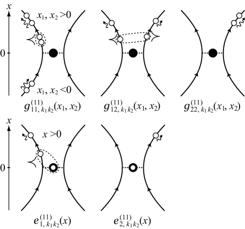
Figure 2: The two-electron scattering eigenfunctions for the incident two electrons coming in through the lead 1. The dotted circles surrounding the two electrons indicate the two-body bound states, which appear only when at least one of the electrons is reflected.

It is instructive to inspect the set of wave numbers characterizing each term of the eigenfunctions in Eqs. (III.2). As is found from the terms of the two-body bound states, the wave-number set $\{k_{1},k_{2}\}$ of the incident states is not conserved and is scattered to the set $\{\epsilon_{\rm d}-\mathrm{i}\Gamma,E-\epsilon_{\rm d}+\mathrm{i}\Gamma\}$ including the imaginary part $\mathrm{i}\Gamma$. We note that the terms of the two-body bound states decay with the distance of the two electrons but are stationary in time since the total energy eigenvalue is real; the imaginary parts of the complex wave numbers cancel out each other in the total energy eigenvalue. By the completeness of the plane-wave functions $\{\mathrm{e}^{\mathrm{i}(k_{1}x_{1}+k_{2}x_{2})}|k_{1},k_{2}\in\mathbb{R}\}$, the terms are expanded as

$$\mathrm{e}^{(\mathrm{i}(\frac{E}{2}-\epsilon_{\rm d})-\Gamma)|x_{1}-x_{2}|+\mathrm{i}E\frac{x_{1}+x_{2}}{2}}=\int dk^{\prime}_{1}dk^{\prime}_{2}\frac{1}{E-E^{\prime}+\mathrm{i}0}c(k^{\prime}_{1},k^{\prime}_{2};x_{1},x_{2})\mathrm{e}^{\mathrm{i}(k^{\prime}_{1}x_{1}+k^{\prime}_{2}x_{2})},$$ (25)

where $E^{\prime}=k^{\prime}_{1}+k^{\prime}_{2}$ and $c(k^{\prime}_{1},k^{\prime}_{2};x_{1},x_{2})$ is the coefficient of the expansion. Hence we find that the terms of the two-body bound states describe the various scattering processes to the sets $\{k^{\prime}_{1},k^{\prime}_{2}\}$ satisfying energy conservation $E=E^{\prime}$. The coefficient $c(k^{\prime}_{1},k^{\prime}_{2};x_{1},x_{2})$ has the poles on the complex $k^{\prime}_{1}$- and $k^{\prime}_{2}$-planes which come from the resonant pole $k=\epsilon_{\rm d}-\mathrm{i}\Gamma$ of the one-electron scattering eigenfunctions in Eqs. (13). Thus the two-body bound states appear as a consequence of one-body resonances Ordonez et al. .

The appearance of such many-body bound states is expected for general open QD systems with localized interactions. We have shown that two-body bound states appear in the Anderson model with spin degrees of freedom Imamura et al. (2009) and the double QD systems Nishino et al. (2012). In Ref. Lebedev et al., 2008, the $N$-electron scattering matrix for another QD system with interactions was explicitly constructed in a real-time representation, where two-electron scattering eigenstates are obtained in an integral form. We speculate that, by evaluating the integral form, two-body bound states similar to ours should appear.

III.3 $N$-electron cases

We can obtain the exact $N$-electron scattering eigenstates for arbitrary $N$. The scattering eigenstates for a few electrons can be constructed in a way similar to the two-electron cases. In the three-electron scattering eigenstates, for example, two electrons out of the three form the two-body bound states after the scattering at the QD Nishino et al. (2009). The explicit form of the scattering eigenstates for a few electrons leads to a conjectural form of the $N$-electron scattering eigenstates. We have shown that they are indeed the eigenstates.

We present only the results in the first order of $U_{\ell}$, which we need in the next section. The form of the $N$-electron scattering eigenstates is given by

$$|E\rangle =\Big{(}\sum_{\{m_{i}\}}\int_{x_{1}<\cdots<x_{N}}d^{N}x\,g_{m_{1}\cdots m_{N}}(x_{1},\ldots,x_{N})c^{\dagger}_{m_{1}}(x_{1})\cdots c^{\dagger}_{m_{N}}(x_{N})$$

$$\quad+\sum_{\{n_{i}\}}\int_{x_{1}<\cdots<x_{N-1}}d^{N-1}x\,e_{n_{1}\cdots n_{N-1}}(x_{1},\ldots,x_{N-1})c^{\dagger}_{n_{1}}(x_{1})\cdots c^{\dagger}_{n_{N-1}}(x_{N-1})d^{\dagger}\Big{)}|0\rangle.$$ (26)

Here we impose the antisymmetric relations for the $N$-electron eigenfunctions as follows:

$$g_{m_{Q_{1}}\cdots m_{Q_{N}}}(x_{Q_{1}},\ldots,x_{Q_{N}})=\mathrm{sgn}(Q)g_{m_{1}\cdots m_{N}}(x_{1},\ldots,x_{N}),$$

$$e_{n_{R_{1}}\cdots n_{R_{N-1}}}(x_{R_{1}},\ldots,x_{R_{N-1}})=\mathrm{sgn}(R)e_{n_{1}\cdots n_{N-1}}(x_{1},\ldots,x_{N-1}),$$ (27)

where $Q=(Q_{1},\ldots,Q_{N})$ is a permutation of $(1,2,\ldots,N)$ and $R=(R_{1},\ldots,R_{N-1})$ is that of $(1,2,\ldots,N-1)$. We consider the situation in which the electron with wave number $k_{i},(i=1,\ldots,N)$ comes in through the lead $\ell_{i}$ to the QD. The $N$-electron scattering eigenfunctions are constructed in the first order of $U_{\ell}$ as

$$g^{(\ell_{1}\cdots\ell_{N})}_{m_{1}\cdots m_{N},k_{1}\cdots k_{N}}(x_{1},\ldots,x_{N})$$

$$=\sum_{P}\mathrm{sgn}(P)\prod_{i=1}^{N}g^{(\ell_{P_{i}})}_{m_{i},k_{P_{i}}}(x_{i})$$

$$\quad+\frac{1}{2}\sum_{P,Q}\mathrm{sgn}(PQ)\prod_{i=1}^{N-2}g^{(\ell_{P_{i}})}_{m_{Q_{i}},k_{P_{i}}}(x_{Q_{i}})\theta(x_{Q_{N-2}},\ldots,x_{Q_{1}})$$

$$\qquad\times t_{m_{Q_{N-1}}}U_{m_{Q_{N}}}Z^{(\ell_{P_{N-1}}\ell_{P_{N}})}_{m_{Q_{N}},k_{P_{N-1}}k_{P_{N}}}(x_{Q_{N-1}Q_{N}})\mathrm{e}^{\mathrm{i}(k_{P_{N-1}}+k_{P_{N}})x_{Q_{N}}}\theta(x_{Q_{N}Q_{N-1}})\theta(x_{Q_{N-1}})$$

$$\quad+O(U^{2}),$$ (28)

where $P$ and $Q$ are permutations of $(1,2,\ldots,N)$, and

$$e^{(\ell_{1}\cdots\ell_{N})}_{n_{1}\cdots n_{N-1},k_{1}\cdots k_{N}}(x_{1},\ldots,x_{N-1})$$

$$=\sum_{P}\mathrm{sgn}(P)\prod_{i=1}^{N-1}g^{(\ell_{P_{i}})}_{n_{i},k_{P_{i}}}(x_{i})e^{(\ell_{P_{N}})}_{k_{P_{N}}}$$

$$\quad+\frac{1}{2}\sum_{P,Q}\mathrm{sgn}(PQ)\prod_{i=1}^{N-3}g^{(\ell_{P_{i}})}_{n_{Q_{i}},k_{P_{i}}}(x_{Q_{i}})e^{(\ell_{P_{N-2}})}_{k_{P_{N-2}}}\theta(x_{Q_{N-3}},\ldots,x_{Q_{1}})$$

$$\qquad\times t_{n_{Q_{N-2}}}U_{n_{Q_{N-1}}}Z^{(\ell_{P_{N-1}}\ell_{P_{N}})}_{n_{Q_{N-1}},k_{P_{N-1}}k_{P_{N}}}(x_{Q_{N-2}Q_{N-1}})\mathrm{e}^{\mathrm{i}(k_{P_{N-1}}+k_{P_{N}})x_{Q_{N-1}}}\theta(x_{Q_{N-1}Q_{N-2}})\theta(x_{Q_{N-2}})$$

$$\quad-\frac{\mathrm{i}}{2}\sum_{P,Q}\mathrm{sgn}(PQ)\prod_{i=1}^{N-2}g^{(\ell_{P_{i}})}_{n_{Q_{i}},k_{P_{i}}}(x_{Q_{i}})\theta(x_{Q_{N-2}},\ldots,x_{Q_{1}})$$

$$\qquad\times U_{n_{Q_{N-1}}}Z^{(\ell_{P_{N-1}}\ell_{P_{N}})}_{n_{Q_{N-1}},k_{P_{N-1}}k_{P_{N}}}(-x_{Q_{N-1}})\mathrm{e}^{\mathrm{i}(k_{P_{N-1}}+k_{P_{N}})x_{Q_{N-1}}}\theta(x_{Q_{N-1}})$$

$$\quad+O(U^{2}),$$ (29)

where $P$ is a permutation of $(1,2,\ldots,N)$ and $Q$ is that of $(1,2,\ldots,N-1)$. Here we have used the notation

$$\theta(x_{m},\ldots,x_{2},x_{1})=\theta(x_{m,m-1})\cdots\theta(x_{32})\theta(x_{21}).$$ (30)

The third term in Eq. (III.3) corresponds to the configuration in which one of the two electrons that form the two-body bound states is on the QD. On the other hand, the second term in Eq. (III.3) corresponds to the configuration in which both of the two electrons that form the two-body bound states are in the leads, which has not appeared in the two-electron scattering eigenfunction $e^{(\ell_{1}\ell_{2})}_{l,k_{1}k_{2}}(x)$ in Eqs. (III.2) only in $g^{(\ell_{1}\ell_{2})}_{l,k_{1}k_{2}}(x_{1},x_{2})$ in Eqs. (III.2). In what follows, we denote the eigenstate obtained by inserting the eigenfunctions in Eqs. (III.3) and (III.3) into Eq. (III.3) by $|k;\ell\rangle=|k_{1},\ldots,k_{N};\ell_{1},\ldots,\ell_{N}\rangle$.

IV Electric current under bias voltages

IV.1 $N$-electron current

By following the three steps of the extension of the Landauer formula given in Sec. II.2, we next calculate the average electric current for the system under finite bias voltages Nishino et al. (2009, 2011). First, we calculate the $N$-electron current, that is, the quantum-mechanical expectation value of the electric-current operator $I$ with the $N$-electron scattering eigenstates $|k;\ell\rangle$. We assume $k_{i}\neq k_{j}$ if $\ell_{i}=\ell_{j}$ and restrict our calculation to the first order of $U_{\ell}$. We need to calculate the following overlap integral:

$$\langle k;\ell|I|k;\ell\rangle =2\mathrm{Im}\Big{(}\int_{x_{1}<\cdots<x_{N-1}}d^{N-1}x\sum_{\ell,\{n_{i}\}}(-1)^{\ell}\frac{|t_{\bar{\ell}}|^{2}}{t^{2}}t_{\ell}$$

$$\quad\times g^{\ast}_{n_{1}\ldots n_{N-1}\ell}(x_{1},\ldots,x_{N-1},0)e_{n_{1}\ldots n_{N-1}}(x_{1},\ldots,x_{N-1})\Big{)},$$ (31)

where $\bar{\ell}=3-\ell$. By inserting the $N$-electron eigenfunctions in Eqs. (III.3) and (III.3) into Eq. (IV.1), we obtain

$$\langle k;\ell|I|k;\ell\rangle$$

$$=\frac{|t_{1}t_{2}|^{2}}{\pi t^{2}}\Big{(}\frac{L}{2\pi}\Big{)}^{N-1}\sum_{i}(-1)^{\ell_{i}}\mathrm{Im}(G_{k_{i}})$$

$$\quad-\Big{(}\frac{L}{2\pi}\Big{)}^{N-2}\sum_{i\neq j}(-1)^{\ell_{i}}\sum_{m}U_{m}\mathrm{Im}\Big{(}\frac{2t_{1}t_{2}}{t^{2}}e^{(\bar{\ell}_{i})}_{k_{i}}g^{(\ell_{j})\ast}_{m,k_{j}}(0+)Z^{(\ell_{i}\ell_{j})}_{\ell,k_{i}k_{j}}(0)\Big{)}$$

$$\quad-\frac{2|t_{1}t_{2}|^{2}}{\pi t^{2}}\Big{(}\frac{L}{2\pi}\Big{)}^{N-3}\sum_{i\neq j\neq l(\neq i)}(-1)^{\ell_{i}}\mathrm{Im}(G_{k_{i}})\sum_{m}U_{m}\mathrm{Re}\big{(}G_{k_{j}}g^{(\ell_{l})\ast}_{m,k_{l}}(0+)e^{(\ell_{j})\ast}_{k_{j}}Z^{(\ell_{j}\ell_{l})}_{m,k_{j}k_{l}}(0)\big{)}$$

$$\quad+O(U^{2}).$$ (32)

Here $L$ is the system length coming from the regularized square norm $\langle k;\ell|k;\ell\rangle=L/(2\pi)$ of the one-electron scattering eigenstates. In order to express the results, we have used the notation

$$G_{k}=\frac{1}{k-\epsilon_{{\rm d}}+\mathrm{i}\Gamma},$$ (33)

which is the one-electron Green’s function on the QD. We notice that the choice of the parameter $\alpha$ in Eqs. (2) simplifies the calculation. On the other hand, the square norm of the $N$-electron eigenstates is calculated as

$$\langle k;\ell|k;\ell\rangle$$

$$=\sum_{\{m_{i}\}}\int_{x_{1}<\cdots<x_{N}}d^{N}x\,|g_{m_{1}\cdots m_{N}}(x_{1},\ldots,x_{N})|^{2}+\sum_{\{n_{i}\}}\int_{x_{1}<\cdots<x_{N-1}}d^{N-1}x\,|e_{n_{1}\cdots n_{N-1}}(x_{1},\ldots,x_{N-1})|^{2}$$

$$=\Big{(}\frac{L}{2\pi}\Big{)}^{N}-2\Big{(}\frac{L}{2\pi}\Big{)}^{N-2}\sum_{i\neq j}\sum_{m=1,2}U_{m}\mathrm{Re}\big{(}G_{k_{i}}g^{(\ell_{j})\ast}_{m,k_{j}}(0+)e^{(\ell_{i})\ast}_{k_{i}}Z^{(\ell_{i}\ell_{j})}_{m,k_{i}k_{j}}(0)\big{)}+O(U^{2}).$$ (34)

It should be noted that the term in the $(N-1)$th order in $L$ does not appear above. Combining Eqs. (IV.1) and (IV.1), we obtain the $N$-electron current as

$$\frac{\langle k;\ell|I|k;\ell\rangle}{\langle k;\ell|k;\ell\rangle}$$

$$=\frac{|t_{1}t_{2}|^{2}}{\pi t^{2}}\frac{2\pi}{L}\sum_{i=1}^{N}(-1)^{\ell_{i}}\mathrm{Im}(G_{k_{i}})$$

$$\quad-\frac{4\pi^{2}}{L^{2}}\sum_{i\neq j}(-1)^{\ell_{i}}\sum_{m=1,2}U_{m}\mathrm{Im}\Big{(}\frac{2t_{1}t_{2}}{t^{2}}e^{(\bar{\ell}_{i})}_{k_{i}}g^{(\ell_{j})\ast}_{m,k_{j}}(0+)Z^{(\ell_{i}\ell_{j})}_{m,k_{i}k_{j}}(0)\Big{)}$$

$$\quad+\frac{2|t_{1}t_{2}|^{2}}{\pi t^{2}}\frac{8\pi^{3}}{L^{3}}\sum_{i\neq j}\mathrm{Im}\big{(}(-1)^{\ell_{i}}G_{k_{i}}+(-1)^{\ell_{j}}G_{k_{j}}\big{)}\sum_{m=1,2}U_{m}\mathrm{Re}\big{(}G_{k_{i}}g^{(\ell_{j})\ast}_{m,k_{j}}(0+)e^{(\ell_{i})\ast}_{k_{i}}Z^{(\ell_{i}\ell_{j})}_{m,k_{i}k_{j}}(0)\big{)}$$

$$\quad+O(U^{2}).$$ (35)

IV.2 Average electric current

Next, we take the reservoir limit of the $N$-electron current in Eq. (IV.1) to obtain the average electric current. We assume that the infinite lead substitutes for a large electron reservoir characterized by the Fermi distribution function $f_{\mu,\beta}(k)=1/(1+\mathrm{e}^{\beta(k-\mu)})$ with a chemical potential $\mu$ and an inverse temperature $\beta$. We also assume that electrons are completely equilibrated in each electron reservoir before being re-emitted towards the QD, which is the main assumption of the extension of the Landauer formula.

In the $N$-electron current in Eq. (IV.1), the $N$-dependence appears only in the upper bounds of the sums on the wave numbers together with the factor $2\pi/L$, which means that we can take the reservoir limit $N_{\ell},L\to\infty$ described in Sec. II.2. It should be noted that the first term in Eq. (IV.1) contains a single sum on $i$ with the factor $2\pi/L$ and the second term contains a double sum on $i$ and $j$ with $(2\pi/L)^{2}$ while the third term is a double sum on $i$ and $j$ with $(2\pi/L)^{3}$ due to the square norm $\langle k;\ell|k;\ell\rangle$ appearing in the denominator. Therefore the third term in Eq. (IV.1) vanishes in the reservoir limit $N_{\ell},L\to\infty$.

In order to investigate the average electric current, we set $\ell_{1}=\cdots=\ell_{N_{1}}=1$ and $\ell_{N_{1}+1}=\cdots=\ell_{N}=2$ in Eq. (IV.1) and relabel $|k;\ell\rangle$ by $|k,h\rangle$ with $h_{i}=k_{N_{1}+i}$, ($1\leq i\leq N_{2}$). The $N$-electron current is rewritten as follows:

$$\frac{\langle k,h|I|k,h\rangle}{\langle k,h|k,h\rangle}=J_{0}+J_{1}+J_{2}+O(U^{2}),$$ (36a)

$$J_{0}=-\frac{2\Gamma_{1}\Gamma_{2}}{\pi\Gamma}\frac{2\pi}{L}\Big{[}\sum_{i=1}^{N_{1}}\mathrm{Im}\big{(}G_{k_{i}}\big{)}-\sum_{i=1}^{N_{2}}\mathrm{Im}\big{(}G_{h_{i}}\big{)}\Big{]},$$ (36b)

$$J_{1}=-\frac{\Gamma_{1}\Gamma_{2}}{\pi^{2}\Gamma}\frac{4\pi^{2}}{L^{2}}\Big{[}U_{1}\sum_{1\leq i\neq j\leq N_{1}}\xi^{(11)}_{k_{i}k_{j}}+\sum_{1\leq i\leq N_{1}\atop 1\leq j\leq N_{2}}\big{(}U_{1}\xi^{(12)}_{k_{i}h_{j}}+U_{2}\xi^{(21)}_{h_{j}k_{i}}\big{)}+U_{2}\sum_{1\leq i\neq j\leq N_{2}}\xi^{(22)}_{h_{i}h_{j}}\Big{]},$$ (36c)

where we use

$$\xi^{(lm)}_{kh} =\mathrm{Im}\Big{[}G_{h}\Big{(}(-1)^{l}\delta_{lm}G_{k}-(-1)^{m}G_{h}+2\mathrm{i}\big{(}(-1)^{l}\Gamma_{m}G^{\ast}_{h}G_{k}-(-1)^{m}\Gamma_{l}G^{\ast}_{k}G_{h}\big{)}\Big{)}\Big{]}$$ (37)

and $\Gamma_{l}=|t_{l}|^{2}/2$. We omit the explicit form of $J_{2}$ in Eq. (36a) since it does not contribute to the average electric current in the reservoir limit $N_{\ell},L\to\infty$. Thus the parts of the $N$-electron current that contribute to the average electric current are detemined by the two-electron scattering eigenstates.

In the reservoir limit $N_{\ell},L\to\infty$, we replace the sums on $k_{i}$ in Eq. (36a) by the integral on $k$ with $f_{\mu,\beta}(k)$ as

$$\frac{2\pi}{L}\sum_{i=1}^{N_{\ell}}J(k_{i})\to\int_{-\Lambda}^{\infty}dk\,f_{\mu_{\ell},\beta_{\ell}}(k)J(k),$$ (38)

where we need to introduce the low-energy cutoff $-\Lambda$ since the local dispersion relation of the lead is bottomless. At zero temperature $(\beta_{\ell}=\infty)$, the average electric current is given by

$$\langle I\rangle =-\frac{2\Gamma_{1}\Gamma_{2}}{\pi\Gamma}\int_{\mu_{2}}^{\mu_{1}}dk\,\mathrm{Im}\big{(}G_{k}\big{)}-\frac{\Gamma_{1}\Gamma_{2}}{\pi\Gamma}\sum_{\ell=1,2}U_{\ell}\int_{-\Lambda}^{\mu_{\ell}}dk\,\Big{(}\int_{-\Lambda}^{\mu_{\ell}}dh\,\xi^{(\ell\ell)}_{kh}+\int_{-\Lambda}^{\mu_{\bar{\ell}}}dh\,\xi^{(\ell\bar{\ell})}_{kh}\Big{)}+O(U^{2}).$$ (39)

We notice that the first term in Eq. (39) reproduces the original Landauer formula in the noninteracting cases. The double summations in Eq. (36c) give double integrals in the second term in Eq. (39), which give a contribution of the Coulomb interactions. Through the integral formulas

$$\int_{-\Lambda}^{\mu_{\ell}}dk\,G_{k} =\frac{1}{2}\log\Big{(}\frac{\epsilon_{\ell}^{2}+1}{\epsilon_{\Lambda}^{2}+1}\Big{)}+\mathrm{i}(\arctan(\epsilon_{\ell})-\arctan(\epsilon_{\Lambda})),$$

$$\int_{-\Lambda}^{\mu_{\ell}}dk\,G_{k}^{2} =\frac{1}{\Gamma}\Big{(}\frac{1}{\epsilon_{\ell}-\mathrm{i}}-\frac{1}{\epsilon_{\Lambda}-\mathrm{i}}\Big{)},$$ (40a)

$$\int_{-\Lambda}^{\mu_{\ell}}dk\,G^{\ast}_{k}G_{k} =-\frac{1}{\Gamma}(\arctan(\epsilon_{\ell})-\arctan(\epsilon_{\Lambda})),$$ (40b)

with $\epsilon_{\ell}=(\epsilon_{\rm d}-\mu_{\ell})/\Gamma$ and $\epsilon_{\Lambda}=(\epsilon_{\rm d}+\Lambda)/\Gamma$, we obtain the average electric current

$$\langle I\rangle =-\frac{2\Gamma_{1}\Gamma_{2}}{\pi\Gamma}j_{-}$$

$$\quad+\frac{\Gamma_{1}\Gamma_{2}}{\pi^{2}\Gamma^{2}}\sum_{\ell=1,2}U_{\ell}\Big{[}\big{(}\Gamma_{\bar{\ell}}j_{-}-\Gamma_{\ell}j_{1}\big{)}\log\Big{(}\frac{\epsilon_{\ell}^{2}+1}{\epsilon_{\Lambda}^{2}+1}\Big{)}+\big{(}\Gamma(\epsilon_{\ell}-\epsilon_{\Lambda})-\Gamma_{\ell}\big{(}2\arctan(\epsilon_{\ell})-j_{\Lambda}\big{)}\big{)}j_{2}\Big{]}$$

$$\quad+O(U^{2}),$$ (41)

where we use the notation

$$j_{-}=\arctan(\epsilon_{1})-\arctan(\epsilon_{2}),\quad j_{\Lambda}=2\arctan(\epsilon_{\Lambda}),$$

$$j_{s}=\frac{\epsilon_{1}^{2-s}}{\epsilon_{1}^{2}+1}-\frac{\epsilon_{2}^{2-s}}{\epsilon_{2}^{2}+1},\quad(s=1,2).$$ (42)

We find that the average electric current $\langle I\rangle$ contains linear and logarithmic divergences in the limit $\Lambda\to\infty$, which is similar to the symmetric case $U_{1}=U_{2}$ Doyon (2007); Nishino et al. (2009, 2011).

IV.3 Universal electric current

We employ a renormalization-group technique to deal with the divergences in the average electric current in Eq. (IV.2). The divergences are due to the bottomless dispersion relation. By the renormalization-group analysis, we zoom into the Fermi energy and thereby discard all details that arise from the specifics of the dispersion relation. As a result, we obtain a universal form of the average electric current.

We devise a Callan-Symanzik equation Doyon (2007); Doyon and Andrei (2006) so that the average electric current may satisfy it. Let us introduce a parameter $D=\Gamma\sqrt{\epsilon_{\Lambda}^{2}+1}$. We can indeed see that, for $D\gg\Gamma,|\epsilon_{\rm d}|$, the average electric current $\langle I\rangle$ in Eq. (IV.2) satisfies

$$\Big{(}D\frac{\partial}{\partial D}+\sum_{\ell=1,2}\beta_{\Gamma_{\ell}}\frac{\partial}{\partial\Gamma_{\ell}}+\beta_{\epsilon_{\rm d}}\frac{\partial}{\partial\epsilon_{\rm d}}\Big{)}\langle I\rangle=0,$$ (43)

where the beta functions $\beta_{\Gamma_{\ell}}$ and $\beta_{\epsilon_{\rm d}}$ are given in the first order of $U_{\ell}$ as

$$\beta_{\Gamma_{\ell}}=-\frac{U_{\ell}}{\pi}\Gamma_{\ell}+O(U^{2}),\quad\beta_{\epsilon_{\rm d}}=-\frac{\bar{U}}{\pi}D+O(U^{2})$$ (44)

with the average interaction $\bar{U}=(U_{1}+U_{2})/2$. The Callan-Symanzik equation of the form (43) is an extension of the previous ones  Doyon (2007); Nishino et al. (2009, 2011) for the case of the symmetric couplings.

The general solution of the Callan-Symanzik equation determines a scaling form of the average electric current as

$$\langle I\rangle=J\Big{(}D^{\frac{U_{1}}{\pi}}\Gamma_{1},D^{\frac{U_{2}}{\pi}}\Gamma_{2},\epsilon_{\rm d}+\frac{\bar{U}}{\pi}D\Big{)},$$ (45)

where $J(\cdot,\cdot,\cdot)$ is an arbitrary three-variable function. Hence, if we change the parameters $\Gamma_{\ell}$ and $\epsilon_{\rm d}$ as functions in $D$ as

$$\Gamma_{\ell}(D)=T_{\ell}\Big{(}\frac{T_{\rm K}}{D}\Big{)}^{\frac{U_{\ell}}{\pi}},\quad\epsilon_{\rm d}(D)=E_{\rm d}-\frac{\bar{U}}{\pi}D$$ (46)

with the constants $T_{1}$, $T_{2}$, ($T_{\rm K}=T_{1}+T_{2}$) and $E_{\rm d}$, the average electric current $\langle I\rangle$ does not depend on $D$. The parameters $\Gamma_{\ell}(D)$ and $\epsilon_{\rm d}(D)$ are referred to as renormalized parameters while the original parameters are called “bare” parameters, which we denote by $\Gamma_{\ell,0}$, $\epsilon_{{\rm d},0}$ and $D_{0}$. Here we fix the renormalized constants $T_{\ell}$ and $E_{\rm d}$ by the bare parameters as

$$T_{\ell}=\Gamma_{\ell,0}\Big{(}\frac{D_{0}}{T_{\rm K}}\Big{)}^{\frac{U_{\ell}}{\pi}},\quad E_{\rm d}=\epsilon_{\rm d}+\frac{\bar{U}}{\pi}D_{0}$$ (47)

and express all physical quantities in terms of the renormalized ones. We shall see below that the sum $T_{\rm K}=T_{1}+T_{2}$ plays a role of a scaling parameter similar to the Kondo temperature.

By inserting the renormalized parameters in Eqs. (46) into the average electric current $\langle I\rangle$ in Eq. (IV.2) and rearranging it with respect to the interaction parameter $U_{\ell}$, we obtain the universal electric current

$$\langle I\rangle =-\frac{2T_{1}T_{2}}{\pi T_{\rm K}}\tilde{j}_{-}$$

$$\quad+\frac{T_{1}T_{2}}{\pi^{2}T^{2}_{\rm K}}\sum_{\ell}U_{\ell}\Big{[}\big{(}T_{\bar{\ell}}\tilde{j}_{-}-T_{\ell}\tilde{j}_{1}\big{)}\log(\tilde{\epsilon}_{\ell}^{2}+1)+\big{(}T_{\rm K}\tilde{\epsilon}_{\ell}-T_{\ell}\big{(}2\arctan(\tilde{\epsilon}_{\ell})-\pi\big{)}\big{)}\tilde{j}_{2}\Big{]}$$

$$\quad+O(U^{2}),$$ (48)

where $\tilde{j}_{-}$ and $\tilde{j}_{s}$ are $j_{-}$ and $j_{s}$ with $\tilde{\epsilon}_{\ell}=(E_{\rm d}-\mu_{\ell})/T_{\rm K}$ in place of $\epsilon_{\ell}$, respectively. Thus the average electric current $\langle I\rangle$, which was originally described by the bare parameters $\Gamma_{\ell,0}$, $\epsilon_{{\rm d},0}$, $D_{0}$ and $U_{\ell}$, is now characterized by the parameters $T_{\ell}$, $E_{\rm d}$ and $U_{\ell}$. As a result, the linear and the logarithmic divergences of the average electric current are absorbed into the parameters $T_{\ell}$ and $E_{\rm d}$.

Let us consider the current-voltage ($I$-$V$) characteristics of the universal electric current. We put $E_{\rm d}=0$ and consider the cases $\mu_{1}=-\mu_{2}=V/2$ with the bias voltage $V$. Then we have

$$\frac{T_{\rm K}}{4T_{1}T_{2}}\langle I\rangle =\frac{1}{\pi}\arctan\Big{(}\frac{V}{2T_{\rm K}}\Big{)}$$

$$\quad-\frac{1}{2\pi^{2}}\Big{[}(\bar{U}-\delta)\arctan\Big{(}\frac{V}{2T_{\rm K}}\Big{)}-(\bar{U}+\delta)\frac{V/(2T_{\rm K})}{V^{2}/(2T_{\rm K})^{2}+1}\Big{]}\log\Big{(}\Big{(}\frac{V}{2T_{\rm K}}\Big{)}^{2}\!\!+1\Big{)}$$

$$\quad+O(U^{2}),$$ (49)

where $\delta$ is the asymmetry parameter defined by

$$\delta=\frac{(U_{1}-U_{2})(T_{1}-T_{2})}{2T_{\rm K}}.$$ (50)

We note that the parameters $T_{1}$ and $T_{2}$ depend on $U_{1}$ and $U_{2}$ through Eqs. (47).

We find from Eq. (IV.3) that the bias voltage $V$ is scaled by the parameter $T_{\rm K}$. In the case of symmetric interactions $U_{1}=U_{2}$, we have $\delta=0$. Hence, after taking appropriate scaling factors for the electric current $\langle I\rangle$ and the bias voltage $V$, the $I$-$V$ curve is independent of the parameters $T_{1}$ and $T_{2}$. In the asymmetric cases with $\Gamma_{1,0}\neq\Gamma_{2,0}$ and $U_{1}\neq U_{2}$, on the other hand, the parameters $T_{1}$ and $T_{2}$ play a nontrivial role since, even if we rescale the electric current, it still depends on $T_{1}$ and $T_{2}$ through the asymmetry parameter $\delta$.

We deal with the parameters $T_{1}$ and $T_{2}$ in the first order of $U_{\ell}$. By solving the equation for $T_{\rm K}$, which is obtained by the first equation in Eqs. (47), the parameter $T_{\ell}$ is expanded in the first order of $U_{\ell}$ as

$$T_{\ell}=\Gamma_{\ell,0}\Big{(}1+\frac{U_{\ell}}{\pi}\log\Big{(}\frac{D_{0}}{\Gamma_{0}}\Big{)}\Big{)}+O(U^{2}).$$ (51)

We remark that, for the consistency with the expansion, the ratio $D_{0}/\Gamma_{0}$ should be restricted to the region $D_{0}/\Gamma_{0}\ll\mathrm{e}^{\pi/U_{\ell}}$. Then the asymmetry parameter $\delta$ in Eq. (50) is expanded as

$$\delta =\frac{(U_{1}-U_{2})(\Gamma_{1,0}-\Gamma_{2,0})}{2\Gamma_{0}}+O(U^{2}).$$ (52)

By a physical intuition, we expect $\delta\geq 0$ since the case $U_{1}>U_{2}$ should correspond to the case $\Gamma_{1,0}>\Gamma_{2,0}$. By expressing the parameters as $\Gamma_{1/2,0}=\Gamma_{0}(1\pm\gamma)/2$ with $0\leq\gamma<1$ and $U_{1/2}=\bar{U}(1\pm\gamma^{\prime})$ with $0\leq\gamma^{\prime}\leq 1$ in the cases with $\Gamma_{1,0}\geq\Gamma_{2,0}>0$ and $U_{1}\geq U_{2}$, we have $\delta=\bar{U}\gamma\gamma^{\prime}+O(U^{2})$. Hence the asymmetry parameter $\delta$ takes a value in the range $0\leq\delta<\bar{U}+O(U^{2})$. The $I$-$V$ curve of the universal electric current for $\bar{U}=0.5$ and $0\leq\delta<0.5$ is depicted in Fig. 3.

We observe the suppression of the electric current for large bias voltages $V\gg T_{\rm K}$, that is, negative differential conductance. This is because the formation of the two-body bound states promotes the reflection of electrons at the QD, as is illustrated in Fig. 2, and the logarithmic term in Eq. (IV.3) decreases the electric current. In the first order of $U_{\ell}$, the negative differential conductance shows the power-law behavior $\langle I\rangle\propto(V/T_{\rm K})^{-(\bar{U}-\delta)/\pi}$ where the asymmetry parameter $\delta$ appears. This means that the suppressed electric current is restored by the asymmetry of the system parameters. In the case $\Gamma_{1,0}=\Gamma_{2,0}$, we have $\delta=0$ in the first order of $U_{\ell}$ and the universal electric current in Eq. (IV.3) depends only on the average interaction $\bar{U}$. This is consistent with the Callan-Symanzik equation: by changing the variables and setting $\Gamma_{1}=\Gamma_{2}=\Gamma/2$, the Callan-Symanzik equation (43) is reduced to

$$\Big{(}D\frac{\partial}{\partial D}+\beta_{\Gamma}\frac{\partial}{\partial\Gamma}+\beta_{\epsilon_{\rm d}}\frac{\partial}{\partial\epsilon_{\rm d}}\Big{)}\langle I\rangle=0$$ (53)

with the beta function $\beta_{\Gamma}=-\bar{U}\Gamma/\pi+O(U^{2})$. The general solution is given in the form $\langle I\rangle=J(D^{\frac{\bar{U}}{\pi}}\Gamma,\epsilon_{\rm d}+\bar{U}D/\pi)$ with an arbitrary two-variable function $J(\cdot,\cdot)$. Then the negative differential conductance appears for $\bar{U}>0$, which is essentially the same as the previous results in the case of symmetric interactions $U_{1}=U_{2}$ Doyon (2007); Boulat et al. (2008); Nishino et al. (2011).

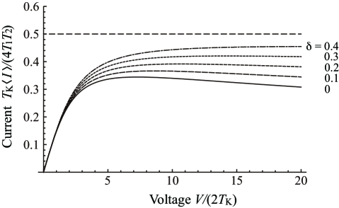
Figure 3: $I$-$V$ characteristics of the rescaled universal electric current for $\bar{U}=0.5$ with $\delta=0,0.1,0.2,0.3,0.4$.

Let us compare the present results with the renormalization-group (RG) results in Refs. C. Karrasch, S. Andergassen, M. Pletyukhov, D. Schuricht, L. Borda, V. Meden, and H. Schoeller, 2010 and S. Andergassen, M. Pletyukhov, D. Schuricht, H. Schoeller, and L. Borda, 2011; the RG flow equations for the level width $\Gamma$ were obtained in the second order of $U_{\ell}$ in Ref. S. Andergassen, M. Pletyukhov, D. Schuricht, H. Schoeller, and L. Borda, 2011. Although general local dispersion relations of the leads were adopted in Refs. C. Karrasch, S. Andergassen, M. Pletyukhov, D. Schuricht, L. Borda, V. Meden, and H. Schoeller, 2010 and S. Andergassen, M. Pletyukhov, D. Schuricht, H. Schoeller, and L. Borda, 2011, the details of the frequency dependence of the density of states of the leads did not play any role in their analysis. Indeed, the linear divergence in our average electric current $\langle I\rangle$ due to the linearized dispersion relations is removed by the RG technique with the Callan-Symanzik equation as we have described above. Their definition of the parameters $T_{1}$ and $T_{2}$, which was approximately derived from the RG flow equations for the level width $\Gamma$, is equivalent to ours in Eq. (47) in the first order of $U_{\ell}$.

We can confirm that the universal electric current in Eq. (IV.3) is consistent with that of the RG results C. Karrasch, S. Andergassen, M. Pletyukhov, D. Schuricht, L. Borda, V. Meden, and H. Schoeller (2010); S. Andergassen, M. Pletyukhov, D. Schuricht, H. Schoeller, and L. Borda (2011) in the first order of $U_{\ell}$. By using the renormalized band width $\Gamma_{\ell}(D)$ in Eq. (46), we have

$$\frac{\Gamma_{1}(D)\Gamma_{2}(D)}{\Gamma(D)}\arctan\Big{(}\frac{V}{2\Gamma(D)}\Big{)}$$

$$=\frac{T_{1}T_{2}}{T_{\rm K}}\Big{[}\arctan\Big{(}\frac{V}{2T_{\rm K}}\Big{)}$$

$$\quad-\!\frac{1}{2\pi}\Big{[}(\bar{U}\!-\!\delta)\arctan\Big{(}\frac{V}{2T_{\rm K}}\Big{)}-(\bar{U}\!+\!\delta)\frac{V/(2T_{\rm K})}{V^{2}/(2T_{\rm K})^{2}\!+\!1}\Big{]}\log\Big{(}\frac{D^{2}}{T^{2}_{\rm K}}\Big{)}\Big{]}+O(U^{2}).$$ (54)

Then, by putting $\tilde{\Gamma}_{\ell}=\Gamma_{\ell}(|V/2+\mathrm{i}T_{\rm K}|)$ and $\tilde{\Gamma}=\tilde{\Gamma}_{1}+\tilde{\Gamma}_{2}$, the universal electric current in Eq. (IV.3) is expressed by

$$\langle I\rangle=\frac{4\tilde{\Gamma}_{1}\tilde{\Gamma}_{2}}{\pi\tilde{\Gamma}}\arctan\Big{(}\frac{V}{2\tilde{\Gamma}}\Big{)}+O(U^{2}),$$ (55)

which is in the same form as the noninteracting cases. The expression in Eq. (55) agrees with that obtained in the RG results (see Appendix A).

We remark that, although the expression of the universal electric current in Refs. C. Karrasch, S. Andergassen, M. Pletyukhov, D. Schuricht, L. Borda, V. Meden, and H. Schoeller, 2010 and S. Andergassen, M. Pletyukhov, D. Schuricht, H. Schoeller, and L. Borda, 2011 agrees with ours in Eq. (55), their treatment of the renormalized parameters $T_{1}$ and $T_{2}$ included in the universal electric current is different from ours; they used the higher-order terms of $U_{\ell}$ in the defining relations of $T_{1}$ and $T_{2}$ in Eq. (47) while we have treated them in the first order of $U_{\ell}$ as is given Eq. (51). As a result, even in the case $\Gamma_{1,0}=\Gamma_{2,0}$ of symmetric lead-dot couplings, they observed the restoration of the suppressed electric current. We have shown that, for the asymmetry parameter $\delta$ treated in the first order of $U_{\ell}$, the restoration due to the asymmetric interactions does not occur at $\Gamma_{1,0}=\Gamma_{2,0}$. In other words, in this case, there should be no restoration of the suppressed electric current for small $U_{\ell}$, which seems to differ from the results of Refs. C. Karrasch, S. Andergassen, M. Pletyukhov, D. Schuricht, L. Borda, V. Meden, and H. Schoeller, 2010 and S. Andergassen, M. Pletyukhov, D. Schuricht, H. Schoeller, and L. Borda, 2011.

V Concluding remarks

We have studied the average electric current for the open QD systems described by the two-lead IRLM in the asymmetric settings. By using the extension of the Landauer formula with the many-electron scattering eigenstates, we have calculated the average electric current for the systems under finite bias voltages. The calculation is in the first order of the interaction parameters, but otherwise we have not employed any approximations. The calculation itself has been considerably simplified compared to the previous one Nishino et al. (2009, 2011) treating the symmetric cases with the even-odd transformation.

Through the renormalization-group technique with the Callan-Symanzik equation, we have obtained the universal electric current characterized by the scaling parameter $T_{\rm K}$ and the asymmetry parameter $\delta$. The Coulomb interactions around the QD give rise to the negative differential conductance through the formation of the two-body bound states, which is a new point of view clarified in our analysis. Through the investigation of the asymmetry parameter $\delta$, we have confirmed in the first order of $U_{1}$ and $U_{2}$ that the suppressed electric current is restored in the asymmetric cases satisfying both $\Gamma_{1,0}\neq\Gamma_{2,0}$ and $U_{1}\neq U_{2}$.

The analytic form of the universal electric current has enabled us to compare it with those of other approaches correctly. Our universal electric current has the same functional form as that obtained with the RG approach C. Karrasch, S. Andergassen, M. Pletyukhov, D. Schuricht, L. Borda, V. Meden, and H. Schoeller (2010); S. Andergassen, M. Pletyukhov, D. Schuricht, H. Schoeller, and L. Borda (2011); it also reproduces previous results Borda et al. (2007); Doyon (2007); Boulat et al. (2008); Golub (2007); Nishino et al. (2011) in the symmetric cases. However, for $U_{1}\neq U_{2}$ and $\Gamma_{1,0}=\Gamma_{2,0}$, our results indicate that there is no restoration of the suppressed electric current to first order in $U_{1}$ and $U_{2}$, while Refs. C. Karrasch, S. Andergassen, M. Pletyukhov, D. Schuricht, L. Borda, V. Meden, and H. Schoeller, 2010 and S. Andergassen, M. Pletyukhov, D. Schuricht, H. Schoeller, and L. Borda, 2011 indicate that there is. This restoration may result from higher-order terms in $U_{1}$ and $U_{2}$. To verify its validity analytically, we need a consistent treatment of these higher-order terms, which can be done with our extension of the Landauer formula.

The key element for the practical calculations in the extension of the Landauer formula is the explicit form of many-electron scattering eigenstates. The present calculation in the first order in the interaction parameters can be extended to higher orders by using the exact $N$-electron scattering eigenstates that we have already obtained. We expect that such calculation should be applied to other physical quantities of the open QD systems such as the dot occupancy.

Appendix A Results of the RG flow equation for $\Gamma$

In our settings, the universal electric current obtained in Refs. C. Karrasch, S. Andergassen, M. Pletyukhov, D. Schuricht, L. Borda, V. Meden, and H. Schoeller, 2010 and S. Andergassen, M. Pletyukhov, D. Schuricht, H. Schoeller, and L. Borda, 2011 is expressed as

$$\langle I\rangle_{\rm RG} =\frac{2\hat{\Gamma}_{1}\hat{\Gamma}_{2}}{\pi\hat{\Gamma}}\Big{[}\arctan\Big{(}\frac{\mu_{1}\!-\!\epsilon_{\rm d}}{\hat{\Gamma}}\Big{)}\!-\!\arctan\Big{(}\frac{\mu_{2}\!-\!\epsilon_{\rm d}}{\hat{\Gamma}}\Big{)}\Big{]},$$ (56)

where $\hat{\Gamma}_{\ell}$ is the solution of the RG flow equations for the level width of the QD and $\hat{\Gamma}=\hat{\Gamma}_{1}+\hat{\Gamma}_{2}$. It was approximately determined by the self-consistent equation

$$\hat{\Gamma}_{\ell}\simeq\Gamma_{\ell,0}\Big{(}\frac{D_{0}}{|\hat{\Gamma}-\mathrm{i}(\mu_{\ell}-\epsilon_{\rm d})|}\Big{)}^{g_{\ell}}$$ (57)

with $g_{\ell}=U_{\ell}/\pi+O(U^{2})$. In the first order of $U_{\ell}$, the approximate solution is given by

$$\hat{\Gamma}_{\ell} \simeq T_{\ell}\Big{(}\frac{T_{\rm K}}{|\hat{\Gamma}-\mathrm{i}(\mu_{\ell}-\epsilon_{\rm d})|}\Big{)}^{\frac{U_{\ell}}{\pi}}+O(U^{2})$$

$$=T_{\ell}\Big{(}\frac{T_{\rm K}}{|T_{\rm K}-\mathrm{i}(\mu_{\ell}-\epsilon_{\rm d})|}\Big{)}^{\frac{U_{\ell}}{\pi}}+O(U^{2})$$

$$=\Gamma_{\ell}(|(\mu_{\ell}-\epsilon_{\rm d})+\mathrm{i}T_{\rm K}|)+O(U^{2}),$$ (58)

where $\Gamma_{\ell}(D)$ is the renormalized level width defined in Eq. (46). By inserting this into Eq. (56) and setting $\mu_{1/2}=\pm V/2$ and $\epsilon_{\rm d}=0$, the expression in Eq. (56) agrees with Eq. (55).

References

- D. Goldhaber-Gordon, Hadas Shtrikman, D. Mahalu, David Abusch-Magder, U. Meirav, and M. A. Kastner (1998) D. Goldhaber-Gordon, Hadas Shtrikman, D. Mahalu, David Abusch-Magder, U. Meirav, and M. A. Kastner, Nature (London) 391, 156 (1998).
- Cronenwett et al. (1998) S. M. Cronenwett, T. H. Oosterkamp, and L. P. Kouwenhoven, Science 281, 540 (1998).
- W. G. van der Wiel, S. De Franceschi, T. Fujisawa, J. M. Elzerman, S. Tarucha, and L. P. Kouwenhoven (2000) W. G. van der Wiel, S. De Franceschi, T. Fujisawa, J. M. Elzerman, S. Tarucha, and L. P. Kouwenhoven, Science 289, 2105 (2000).
- Andrey V. Kretinin, Hadas Shtrikman, David Goldhaber-Gordon, Markus Hanl, Andreas Weichselbaum, Jan von Delft, Theo Costi, and Diana Mahalu (2011) Andrey V. Kretinin, Hadas Shtrikman, David Goldhaber-Gordon, Markus Hanl, Andreas Weichselbaum, Jan von Delft, Theo Costi, and Diana Mahalu, Phys. Rev. B 84, 245316 (2011).
- A. Yacoby, M. Heiblum, D. Mahalu, and Hadas Shtrikman (1995) A. Yacoby, M. Heiblum, D. Mahalu, and Hadas Shtrikman, Phys. Rev. Lett. 74, 4047 (1995).
- R. Schuster, E. Buks, M. Heiblum, D. Mahalu, V. Umansky, and Hadas Shtrikman (1997) R. Schuster, E. Buks, M. Heiblum, D. Mahalu, V. Umansky, and Hadas Shtrikman, Nature 385, 417 (1997).
- Datta (1995) S. Datta, Electronic Transport in Mesoscopic Systems (Cambridge University Press, Cambridge, 1995).
- Imry (2002) Y. Imry, Introduction to Mesoscopic Physics, 2nd ed. (Oxford Univ. Pr., Oxford, 2002).
- Yurke and Kochanski (1990) B. Yurke and G. P. Kochanski, Phys. Rev. B 41, 8184 (1990).
- M. Büttiker (1992) M. Büttiker, Phys. Rev. B 46, 12485 (1992).
- Blanter and M. Büttiker (2000) Y. M. Blanter and M. Büttiker, Phys. Rep. 336, 1 (2000).
- C. Caroli, R. Combescot, P. Nozieres, and D. Saint-James (1971) C. Caroli, R. Combescot, P. Nozieres, and D. Saint-James, J. Phys. C: Solid State Phys. 4, 916 (1971).
- Meir et al. (1991) Y. Meir, N. S. Wingreen, and P. A. Lee, Phys. Rev. Lett. 66, 3048 (1991).
- Meir and Wingreen (1992) Y. Meir and N. S. Wingreen, Phys. Rev. Lett. 68, 2512 (1992).
- Hershfield et al. (1992) S. Hershfield, J. H. Davies, and J. W. Wilkins, Phys. Rev. B 46, 7046 (1992).
- Haug and Jauho (2007) H. Haug and A. P. Jauho, Quantum Kinetics in Transport and Optics of Semiconductors, 2nd ed. (Springer, Berlin, 2007).
- Ng and Lee (1988) T. K. Ng and P. A. Lee, Phys. Rev. Lett. 61, 1768 (1988).
- Wingreen and Meir (1994) N. S. Wingreen and Y. Meir, Phys. Rev. B 49, 11040 (1994).
- Nishino et al. (2009) A. Nishino, T. Imamura, and N. Hatano, Phys. Rev. Lett. 102, 146803 (2009).
- Nishino et al. (2011) A. Nishino, T. Imamura, and N. Hatano, Phys. Rev. B 83, 035306 (2011).
- Filyov and Wiegmann (1980) V. M. Filyov and P. B. Wiegmann, Phys. Lett. A 76, 283 (1980).
- Mehta and Andrei (2006) P. Mehta and N. Andrei, Phys. Rev. Lett. 96, 216802 (2006).
- Borda et al. (2007) L. Borda, K. Vladár, and A. Zawadowski, Phys. Rev. B 75, 125107 (2007).
- Doyon (2007) B. Doyon, Phys. Rev. Lett. 99, 076806 (2007).
- Boulat et al. (2008) E. Boulat, H. Saleur, and P. Schmitteckert, Phys. Rev. Lett. 101, 140601 (2008).
- Doyon and Andrei (2006) B. Doyon and N. Andrei, Phys. Rev. B 73, 245326 (2006).
- Golub (2007) A. Golub, Phys. Rev. B 76, 193307 (2007).
- Aharony et al. (2000) A. Aharony, O. Entin-Wohlman, and Y. Imry, Phys. Rev. B 61, 5452 (2000).
- Goorden and M. Büttiker (2007) M. C. Goorden and M. Büttiker, Phys. Rev. Lett. 99, 146801 (2007).
- Lebedev et al. (2008) A. V. Lebedev, G. B. Lesovik, and G. Blatter, Phys. Rev. Lett. 100, 226805 (2008).
- C. Karrasch, S. Andergassen, M. Pletyukhov, D. Schuricht, L. Borda, V. Meden, and H. Schoeller (2010) C. Karrasch, S. Andergassen, M. Pletyukhov, D. Schuricht, L. Borda, V. Meden, and H. Schoeller, Eur. Phys. Lett. 90, 30003 (2010).
- S. Andergassen, M. Pletyukhov, D. Schuricht, H. Schoeller, and L. Borda (2011) S. Andergassen, M. Pletyukhov, D. Schuricht, H. Schoeller, and L. Borda, Phys. Rev. B 83, 205103 (2011).
- (33) D. Schuricht, private communication.
- Imamura et al. (2009) T. Imamura, A. Nishino, and N. Hatano, Phys. Rev. B 80, 245323 (2009).
- Nishino et al. (2012) A. Nishino, T. Imamura, and N. Hatano, J. Phys.: Conf. Ser. 343, 012087 (2012).
- Hershfield (1993) S. Hershfield, Phys. Rev. Lett. 70, 2134 (1993).
- Han (2006) J. E. Han, Phys. Rev. B 73, 125319 (2006).
- Anders (2008) F. B. Anders, Phys. Rev. Lett. 101, 066804 (2008).
- Schiller and Hershfield (1995) A. Schiller and S. Hershfield, Phys. Rev. B 51, 12896 (1995).
- Schiller and Hershfield (1998) A. Schiller and S. Hershfield, Phys. Rev. B 58, 14978 (1998).
- Shen and Fan (2007) J. T. Shen and S. Fan, Phys. Rev. Lett. 98, 153003 (2007).
- (42) G. Ordonez, A. Nishino, and N. Hatano, unpublished.