Montblanc: GPU accelerated
Radio Interferometer Measurement Equations
in support of
Bayesian Inference for Radio Observations

Abstract

We present Montblanc, a GPU implementation of the Radio interferometer measurement equation (RIME) in support of the Bayesian inference for radio observations (BIRO) technique. BIRO uses Bayesian inference to select sky models that best match the visibilities observed by a radio interferometer. To accomplish this, BIRO evaluates the RIME multiple times, varying sky model parameters to produce multiple model visibilities. $\chi^{2}$ values computed from the model and observed visibilities are used as likelihood values to drive the Bayesian sampling process and select the best sky model.

As most of the elements of the RIME and $\chi^{2}$ calculation are independent of one another, they are highly amenable to parallel computation. Additionally, Montblanc caters for iterative RIME evaluation to produce multiple $\chi^{2}$ values. Modified model parameters are transferred to the GPU between each iteration.

We implemented Montblanc as a Python package based upon NVIDIA’s CUDA architecture. As such, it is easy to extend and implement different pipelines. At present, Montblanc supports point and Gaussian morphologies, but is designed for easy addition of new source profiles.

Montblanc’s RIME implementation is performant: On an NVIDIA K40, it is approximately 250 times faster than MeqTrees on a dual hexacore Intel E5–2620v2 CPU. Compared to the OSKAR simulator’s GPU-implemented RIME components it is 7.7 and 12 times faster on the same K40 for single and double-precision floating point respectively. However, OSKAR’s RIME implementation is more general than Montblanc’s BIRO-tailored RIME.

Theoretical analysis of Montblanc’s dominant CUDA kernel suggests that it is memory bound. In practice, profiling shows that is balanced between compute and memory, as much of the data required by the problem is retained in L1 and L2 cache.

1 Introduction

Bayesian inference for radio observations (BIRO) (Lochner et al., 2015) is a rigorous statistical technique for inferring a model of the sky brightness distribution from the observed visibilities of a radio interferometer. Such models are composed of various radio sources characterised by physical parameters. For example, point sources are parameterised by position, flux density (in total intensity and polarization) and a spectral index, while extended sources require additional shape parameters. An example sky model is shown in Figure 1c. BIRO explores the full posterior probability distribution of the model parameters given the observed visibility data via MCMC sampling.

(a) Antennas and baselines

(b) Visibility tracks

(c) Sky model

Figure 1: (a) Radio Interferometers are formed from multiple antennas. Radio signals are measured and correlated on baselines formed between antenna pairs. (b) As the Earth rotates, visibilities are observed in the spatial frequency domain, forming distinctive tracks. (c) BIRO attempts to find a sky model, composed of point and Gaussian sources, whose model visibilities are closest to the interferometer’s observed visibilities (Thompson et al., 2007).

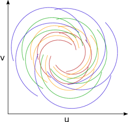
Source extraction via imaging techniques must transform observed visibilities (Figure 1b) into a dirty image, that must be processed by deconvolution algorithms such as clean (Högbom, 1974). Artifacts can be introduced by these algorithms when they attempt to remove the synthesised beam. The noise in this domain must be correlated and is not uniform across the image. Sidelobes and choice of baseline weighting complicate analysis. Sources are subsequently extracted from the map and characterized using, for example, AIPS SAD, SExtractor(E. Bertin and S. Arnouts, 1996) and PyBDSM(Mohan and Rafferty, 2015). By contrast, BIRO uses Bayesian inference to find a sky model that best fits the observed visibility data, given the measurement uncertainties. Central to this process is the conversion of the sky model to model visibilities which, in combination with observed visibilities, produce a $\chi^{2}$ value (goodness of fit) that drives the Bayesian inference process. Performing comparisons in the visibility domain is advantageous since the noise is Gaussian, uncorrelated and stationary (Feroz et al., 2009b). BIRO therefore offers a simple, rigorous, powerful and flexible approach to modelling the sky, bypassing the need for the deconvolution, imaging and source-extraction steps.

The conversion of sky model to model visibilities is governed by the Van Cittert–-Zernike theorem (Thompson et al., 2007), which provides the basis for modelling an interferometer’s response to a radio source. Established models based on this theorem are only suited to older calibration techniques that incorporate direction-independent effects (DIEs). However, they are increasingly unsuitable for newer, more sensitive telescopes whose wide-field/wide-band nature make them susceptible to subtler direction-dependent effects (DDEs). The Radio Interferometer Measurement Equation (RIME) (Hamaker et al., 1996; Smirnov, 2011a) reformulates the Van Cittert–Zernike theorem using Jones calculus and provides a rigorous basis for modelling current and future interferometers and effects. Due to this power and flexibility, it is the RIME that BIRO makes use of to convert the sky brightness distribution into model visibilities. This even permits calibration to be undertaken simultaneously with modelling of the sky.

Existing BIRO implementations Lochner et al. (2015) use MeqTrees (Noordam and Smirnov, 2010) to evaluate the RIME, and (for example) MultiNEST (Feroz et al., 2009a) for performing Bayesian parameter estimation and model selection. However, the parameter space that BIRO must explore can be large (10 to 100 parameters at present, 1000 to 10000 are planned in future) and often unusually shaped, resulting in tens of thousands of RIME evaluations. Furthermore, a single RIME evaluation is expensive, since visibilities must be calculated over time, baseline and channel, before reduction to a single $\chi^{2}$ value. Fortunately, these values can be independently calculated, rendering the RIME particularly amenable to a parallel implementation, accelerated by Graphics Programming Units (GPUs).

The likelihood values used by Bayesian inference are computed from the $\chi^{2}$ values and inform the sky model selection process. These calculations are not only relevant to BIRO. Paraphrasing (Kazemi et al., 2011), telescope calibration can be thought of as Maximum-likelihood (ML) estimation MacKay (2003) of instrument and sky parameters through non-linear optimisation techniques, such as Levenberg-Marquardt (Levenberg, 1944; Marquardt, 1963). Radio astronomy packages such as CASA(Tran and Winkler, 2014) and MeqTrees (Noordam and Smirnov, 2010) implement ML to perform calibration, and also rely on computation of the RIME and $\chi^{2}$. Such techniques also benefit from a fast RIME implementation.

OSKAR (Mort et al., 2010) is a radio interferometer simulator that implements certain parts of the RIME in NVIDIA’s CUDA (NVIDIA Corporation, 2014a) architecture and other parts in C. While full-featured, it is a one-shot simulator and not designed for iterative evaluation of the RIME, where only relevant sky parameters are changed between BIRO iterations. Additionally, it does not currently support GPU calculation of a $\chi^{2}$ value from the RIME and, due to the specialist nature of the C programming language, it is not particularly easy to add new source types, or extend.

This paper presents Montblanc, a GPU implementation of both the RIME, and a calculator of the $\chi^{2}$ value from the RIME. In contrast to OSKAR, we aim to implement the entire RIME on a GPU. Implemented as a Python package, it in turn uses the PyCUDA (Klöckner et al., 2012) package to access NVIDIA’s CUDA architecture (NVIDIA Corporation, 2014a). Using Montblanc, the time required to calculate the RIME, and the likelihood associated with a model parameter set is dramatically reduced. Montblanc currently supports both point and Gaussian sources, and is architected for the addition of further source types, such as the $\beta$-profile (King, 1966, 1972), the NFW (Navarro et al., 1997) profile and corkscrews. A contributor (Rivi, 2015) has already added Sersic profiles (Sérsic, 1963) for instance. It also supports time-varying brightness and modelling of the beam profile, pointing solution and the noise covariance matrix. At present, it only supports the expression of the DDE term as an analytic equation. DIE matrices are not currently supported since BIRO generally operates on fully calibrated data. Future support for these terms would enable self-calibration simultaneously with sky model selection.

At present, Montblanc provides an in-core solution to the RIME — the problem size, generally governed by the number of visibilities, must fit within the RAM of a compute node. This is not currently problematic for BIRO as time- and/or frequency-averaging (see e.g. (Thompson et al., 2007)) can readily be applied post-flagging to compress the data and hence reduce the computational load. The degree of averaging that can be applied with loss of information is set by the physics of the telescope in question See e.g. (Hobson and Maisinger, 2002; Feroz et al., 2009b).

The text is organised as follows: we first describe the RIME and BIRO technique in more detail and provide an overview of GPU computing and NVIDIA’s CUDA architecture. This is followed by a discussion of existing RIME implementations, MeqTrees and OSKAR. We then describe Montblanc’s architecture, the process for computing the RIME, as well as the process for subdividing the RIME so that the problem will fit within memory budgets. We then present and discuss our results before concluding and mentioning directions for future work.

2 Background

In this section we describe the Radio Interferometry Measurement Equation (RIME), Bayesian Inference for Radio Observations (BIRO) as well as GPUs and NVIDIA’s CUDA architecture.

2.1 The Radio Interferometry Measurement Equation

name	number of	name	number of
ntime	timesteps	nsrc	sources
nbl	baselines	npsrc	point sources
na	antennas	ngsrc	gaussian sources
nchan	channels

Table 1: RIME dimensions referred to in this work.

The Radio Interferometry Measurement Equation was developed by Hamaker et. al. (Hamaker et al., 1996) and revisited in a series of papers by Smirnov (Smirnov, 2011a). It establishes a relation between a sky brightness distribution and the response this produces in an interferometer. The sky model is defined by radio sources and the effects modifying their propagation along the line of sight. By contrast, the interferometer response is measured as complex voltages on an interferometer’s correlated baselines.

The RIME is based on Jones calculus, originally developed to model the polarisation of light by linear optical elements and applied here to radio signals. Jones calculus models radio signals as 2-element complex vectors describing the transverse components of an EM plane wave, and 2x2 complex Jones matrices describing propagation effects. Consequently, the RIME is well-suited to rigorously defining signal propagation effects along the line of sight (Smirnov, 2011b). We use the following formulation of the RIME over nsrc sources:

$$V_{tpq\lambda}=G_{tp\lambda}\left(\sum^{\textrm{nsrc}}_{s=0}E_{tps\lambda}K_{tps\lambda}B_{s\lambda}K_{tqs\lambda}^{H}E_{tqs\lambda}^{H}\right)G_{tp\lambda}^{H},$$ (1)

where $V_{tpq\lambda}$ are the visibilities along the baseline formed by antennas $p$ and $q$, at timestep $t$ and channel with wavelength $\lambda$. $G_{tp\lambda}$ is antenna $p$’s DIE Jones matrix, $E_{tps\lambda}$, the DDE matrix for source $s$, $K_{tps\lambda}$, the phase matrix, and $B_{s\lambda}$, the brightness matrix for source $s$. In general, $G_{tp\lambda}$ and $E_{tps\lambda}$ are matrices that may represent the linear product of more specific propagation effects. A hermitian transpose ($H$) is applied to the corresponding terms for antenna $q$. The formulation above expresses the product and reduction of a 4D array of 2x2 matrices with dimensions of time, antennas, baseline, sources and channel. For the sake of readability we sometimes exclude time and channel in this paper.

While these terms are generally expressed as complex matrices and scalars, analytic expressions can be substituted, trading memory storage, access and transfer costs for the computation of a tensor product. For example, the brightness matrix $B_{s\lambda}$ corresponding to astrophysical sources can typically be parameterised as

$$B_{s\lambda}=\left(\frac{\lambda_{ref}}{\lambda}\right)^{\alpha}\left(\begin{array}[]{cc}I_{s}+Q_{s}&U_{s}+iV_{s}\\ U_{s}-iV_{s}&I_{s}-Q_{s}\end{array}\right),$$ (4)

where $I_{s},Q_{s},U_{s},V_{s}$ are Stokes parameters for source $s$ at reference wavelength $\lambda_{ref}$. Most extragalactic radio sources emit though the synchrotron process, and their spectrum is modeled well by Equation 4 for moderately wide frequency ranges. To first order, most radio sources can be modelled extremely comprehensively using a single spectral index $\alpha$. This holds not only for the most common form of extragalactic emission (synchroton radiation, $\alpha\simeq-0.7$), but also for thermal (cosmic microwave background and/or Sunyaev–Zel’dovich effect) and free-free radiation. Higher-order spectral-index curvature terms, whose effects become significant for moderately-wide bandwidths, could easily be incorporated analytically.

$$K_{tps\lambda}=\mathrm{e}^{\frac{2\pi i}{\lambda}\left(ul+vm+w(n-1)\right)},$$ (5)

where $u_{tp}=(u,v,w)$ is the uvw coordinate for antenna $p$ at time $t$, and $l_{s}=(l,m,n)$ the sky coordinate for source $s$, with $n=\sqrt{1-l^{2}-m^{2}}$. A common analytic approximation for the primary beam profile $E_{ps}$ of the Westerbork Synthesis Radio Telescope (WSRT)(Popping and Braun, 2008; Smirnov, 2011b) is reasonably approximated as

$$E_{ps}=\textrm{cos}^{3}\left(C\lambda\|l_{s}-\Delta l_{p}\|\right),$$ (6)

where $\Delta l_{p}$ is the pointing error for antenna $p$ and $C$=65 GHz is a constant. While this expression applies to Westerbork, others could be substituted, depending on the case. For example, the VLA beam profile can be approximated with a Jinc (Smirnov, 2011b) function. Note that such analytic expressions contain many expensive trigonometric and transcendental functions.

Figure 2: The tensor product, $K_{tps\lambda}$, is created by combining the uvw coordinate $u_{tp}$, the source coordinate $l_{s}$ and the wavelength $\lambda$ (not shown).

Finally, the source coherency is defined as

$$X_{pqs}=E_{ps}K_{ps}B_{s}K_{qs}^{H}E_{qs}^{H},$$ (7)

and by summing over the number of sources, we can obtain the model visibilities along baseline $pq$:

$$X_{pq}=\sum^{nsrc}_{s=0}X_{pqs}.$$ (8)

The model visibilities produced by the RIME can then be compared against the actual observed visibilities of the telescope (see below).

2.2 RIME Dimensions and Parallelism

It is useful to consider the dimensionality of the RIME, since this reveals the inherent parallelism of the equation. As discussed in the previous section, the primary dimensions involved in solving the RIME are timesteps, antennas, baselines, sources and channels. We refer to these dimensions as ntime, na, nbl, nsrc and nchan respectively (Table 1).

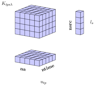
Consider the phase term, $K_{tps\lambda}=\exp\left[(2\pi/\lambda)(u_{tp}\cdot l_{s})\right]$ with input wavelength $\lambda$ ($\mathtt{nchan}$), uvw coordinate $u_{tp}$ ($\mathtt{ntime\times na}$) and source coordinate $l_{s}$ ($\mathtt{nsrc}$). Then, the tensor product of these inputs $K_{tps\lambda}$ (Figure 2), has dimension $\mathtt{ntime\times na\times nsrc\times nchan}$. The values of this 4D tensor can be computed entirely independently of one another.

Per-antenna terms $K_{tps\lambda}$ and $K_{tqs\lambda}^{H}$ with dimension $\mathtt{ntime\times na\times nsrc\times nchan}$ are combined to produce a $\mathtt{ntime\times nbl\times nsrc\times nchan}$ per-baseline term $K_{tpqs\lambda}$: Each antenna is combined with every other antenna to form $\mathtt{nbl}=\mathtt{na}(\mathtt{na}-1)/2$ baselines, discarding auto-correlations where $p=q$.

Thus to solve the RIME, a $\mathtt{ntime\times nbl\times nsrc\times nchan}$ source-coherency array is computed from the product of tensors. The source dimension of this array is reduced to produce a $\mathtt{ntime\times nbl\times nchan}$ model visibility array. Each value of the source coherency, and each sum over its three dimensions can be computed independently. It is the independence inherent in this calculation, and the dimensionality of the problem, that make the RIME particularly suitable to parallel implementation (section 4.5).

2.3 Bayesian Inference for Radio Observations

Bayesian inference is a method for estimating the set of model parameters $\mathbf{\Theta}$ describing a model or hypothesis $\mathbf{H}$ that includes any assumptions, for data $\mathbf{D}$. Bayes’ theorem states that

$$Pr\left(\mathbf{\Theta}|\mathbf{D},\mathbf{H}\right)=\frac{Pr\left(\mathbf{D}|\mathbf{\Theta},\mathbf{H}\right)Pr\left(\mathbf{\Theta}|\mathbf{H}\right)}{Pr\left(\mathbf{D}|\mathbf{H}\right)}.$$ (9)

$Pr\left(\mathbf{\Theta}|\mathbf{D},\mathbf{H}\right)\equiv P\left(\mathbf{\Theta}|\mathbf{D}\right)$ is the posterior probability distribution of the parameters, $Pr\left(\mathbf{D}|\mathbf{\Theta},\mathbf{H}\right)\equiv\mathcal{L}\left(\mathbf{D}|\mathbf{\Theta}\right)$ the likelihood, $Pr\left(\mathbf{\Theta}|\mathbf{H}\right)\equiv\pi\left(\mathbf{\Theta}\right)$ the prior probability distribution and $Pr\left(\mathbf{D}|\mathbf{H}\right)\equiv\mathcal{Z}\left(\mathbf{D}\right)$ the evidence.

The posterior $P\left(\mathbf{\Theta}|\mathbf{D}\right)$ is the probability distribution of the parameters for the hypothesis or model. In the case of BIRO this refers to the probability that the parameter set governing a particular configuration/instance of the RIME produces model visibilities that match the observed visibilities. The likelihood $\mathcal{L}\left(\mathbf{D}|\mathbf{\Theta}\right)$ is the probability that the data or model is correct, given a set of parameters. Under the assumption of Gaussian measurement uncertainties, this is a $\chi^{2}$ value created by comparing the model visibilities with the observed visibilities $D_{pq}$, given a weight vector $w_{pq}$:

$$-2\ln\mathcal{L}\left(\mathbf{D}|\mathbf{\Theta}\right)=\sum w_{pq}\left(V_{pq}-D_{pq}\right)^{2}+\sum\ln\left(2\pi/w_{pq}\right)=\chi^{2}+\sum\ln\left(2\pi/w_{pq}\right).$$ (10)

The prior $\pi\left(\mathbf{\Theta}\right)$ is the pre-existing probability that the parameter set matches the hypothesis or model, while, $\mathcal{Z}\left(\mathbf{D}\right)$ described below, is the evidence for the data.

Similar to the RIME, this process of calculating the $\chi^{2}$ value involves differencing, squaring and multiplying the individual elements of three $\mathtt{ntime\times nbl\times nchan}$) arrays. As such, it is also a highly parallel operation.

Bayesian inference can also be used to perform model selection. In BIRO’s case for example, this involves choosing the model of the sky that best matches the observed visibilities. This may be a particular combination of point and Gaussian sources. Here the objective is to find the evidence $\mathcal{Z}\left(\mathbf{D}\right)$, the factor required to normalise the posterior over parameter space $\mathbf{\Theta}$:

$$\mathcal{Z}\left(\mathbf{D}\right)=\int\mathcal{L}\left(\mathbf{D}|\mathbf{\Theta}\right)\pi\left(\mathbf{\Theta}\right)d^{D}\mathbf{\Theta},$$ (11)

where $D$ is the dimensionality of parameter space. A salient feature of Bayesian model selection is that it follows Occam’s Razor: it chooses more compact parameter spaces over larger ones, rewarding a good fit but penalizing more complex models. When comparing two models, the ratio of the posteriors $R$, given the observed data set $\mathbf{D}$, is used to select the one with the higher probability:

$$R=\frac{Pr(H_{1}|\mathbf{D})}{Pr(H_{2}|\mathbf{D})}.$$ (12)

2.4 GPUs and CUDA

Prior to 2005 (Barsdell et al., 2010), computing power followed Moore’s Law (Moore, 1965), increasing in direct proportion to increases in Central Processing Unit (CPU) clock rates. However, physical limitations in the manufacturing process prevent further advances with this strategy. Chip manufacturers therefore resorted to providing further compute power by introducing multiple cores on a CPU. Dual, quad, hexacore and octocore CPUs are now ubiquitous.

This strategy is most evident in the architecture of Graphics Programming Units (GPU). GPUs have thousands of cores devoted to rendering billions of pixels. Tens of thousands of threads execute a common shader program on separate pixel data. These shaders are classed as Single Instruction, Multiple Data Streams (SIMD) in Flynn’s Taxonomy (Flynn, 1972) and their computation is highly parallel.

NVIDIA’s Compute Unified Device Architecture (CUDA) (NVIDIA Corporation, 2014a) generalises GPU programming to non-graphics related programs.The parallel nature of many Radio Astronomy (Barsdell et al., 2010) algorithms make them amenable to GPU implementation. Instead of shader programs, CUDA kernels are written in a variant of C. Each kernel executes many threads, grouped into separate thread blocks for execution on GPU cores. Each core executes a group of 32 threads called a warp.

The NVIDIA Kepler K40 consists of 15 streaming multiprocessors (SMX), each containing 192 cores for a total of 2880 cores. Each SMX has 65,536 registers, 64KB of L1 memory, split 16KB/48KB between L1 cache and shared memory configurations, as well as a 48KB read-only L1 cache. An additional 1536KB of L2 cache is shared by all SMXs (NVIDIA Corporation, 2014b).

The amount of theoretical processing power of GPUs is high: A K40’s peak single floating point performance is 4290 GFLOPS/s, more than $10\times$ the 371 GFLOPS/s available to a dual 2.90GHz Intel E5–2690 CPU. In practice, such performance can only be attained by kernels composed of fused multiply-adds (FMA), performed on data in registers and most kernels will not conform to this pattern. Additionally, processor speeds have increased at a far greater rate, compared to memory access speeds. Many operations can occur while waiting for a memory read, but this in turn leads to situations where data dependent algorithms “starve” a processor (Alted, 2010). To ameliorate this, GPUs support high memory bandwidth: memory read latency is amortised via large data transfers and processors waiting for data are assigned other computation. A K40 can read 288 GB/s and the NVIDIA Pascal architecture is projected to provide $\approx 12000$ GFLOPS/s with a memory bandwidth of $\approx 1000$ GB/s. By contrast a E5–2690 has a bandwidth of 51.2 GB/s.

Therefore, approaching a GPU’s (or CPU’s) peak performance is highly dependent on an algorithm’s arithmetic intensity – the number of FLOPS performed per bytes read. To approach this performance, it is necessary to exploit a device’s memory architecture as far as possible. In practice, this means ameliorating and avoiding high latency reads of the GPU’s global memory, firstly by ensuring that threads access contiguous memory locations to achieve coalesced reads. Secondly, as much of the problem as possible should be retained in fast registers, shared memory and cache.

Due to the limited registers and shared memory per SMX, there is a trade-off between the number of threads executed on a SMX, and the registers and shared memory used by each thread. It is desirable for a kernel to exhibit high occupancy by executing as many threads as possible on a SMX since this fully exploits a device’s parallelism. However, high occupancy tends to limit (performant) kernel complexity, as the amount of registers and shared memory available to each thread is reduced.

3 Previous Work

Both MeqTrees (Noordam and Smirnov, 2010) and OSKAR (Mort et al., 2010) are packages that implement the RIME in order to generate visibilities from a parametric sky model.

The goal of MeqTrees is to provide a tool for the rapid development of Radio Astronomy models. It is primarily designed to evaluate the RIME for purposes of telescope simulation and/or calibration the RIME, through the use of expression trees. This representation supports decomposition of the RIME into separate pieces of work for parallel execution over multiple CPU threads. Its back-end is implemented in C++, while Python allows for developers to rapidly prototype on the front-end.

OSKAR is implemented in both C and CUDA. OSKAR’s solution to the RIME is designed for generality – some RIME components are implemented as separate CUDA kernels, while others are implemented on the CPU. The results from these components are multiplied together by CUDA kernels or CPU functions and correlated with one another.

In contrast to direct evaluation of the RIME (which is effectively a DFT), it is possible to use an FFT in combination with convolutional degridding (Cornwell et al., 2008) to obtain model visibilities, given a rasterised sky model image. For example, CASA’s (Tran and Winkler, 2014) imaging functionality could be used to calculate a $\chi^{2}$, although this is not currently implemented in the API.

Both the MeqTrees and OSKAR2 simulators are mature, but are not designed to iteratively evaluate the RIME on a GPU. This is not ideal for BIRO’s case, since, in order to calculate the many $\chi^{2}$ values associated with different parameters, multiple, iterative RIME evaluations are necessary each producing model visibilities. Additionally, they do not, as yet, have the facility to compute a $\chi^{2}$ from model and observed visibilities at each step of the sampling chain. This highly parallel computation would also benefit from GPU implementation.

The FFT approach is not ideal for BIRO for a several reasons. First, discretising/rasterising radio sources defined by continuous parameters requires rasterisation and this image must be continually recreated to account for changing source parameters. At present, the effect of source averaging on the parametric process is not well-understood. Second, degridding must be applied to extract per-time, -baseline and -channel visibilities from the gridded visibilities, introducing further averaging error into the process. Third, while the degridding approach has an inexpensive FFT — $O(N^{2}\,\textrm{log}\,N^{2})$ for an $N\times N$ image — the computational complexity of degridding itself is $O(\mathtt{nvis\times c^{2}})$ vs $O(\mathtt{nvis\times nsrc})$ for the RIME (see Section 5.1) where nvis, c and nsrc are the number of visibilities, convolution support size and number of sources, respectively. Thus, the complexity of the two approaches only differ by the square of the convolution support size and the number of sky model sources — a $256\times 256$ kernel corresponds to 65,536 sources, for instance. This number of sources is more than reasonable for current BIRO requirements, as each of their parameters must be allowed to vary. The degridding approach may indeed be useful for scenarios where radio sources can not be described analytically, or for cases involving many faint sources. However, BIRO does not at present support unparameterised radio-sources.

name	dimensions	type	from MS
uvw	$\mathtt{ntime\times na}$	float	$\checkmark$
antenna pairs	$\mathtt{ntime\times nbl}$	integer	$\checkmark$
lm	$\mathtt{nsrc}$	float	$\times$
brightness	$\mathtt{ntime\times nsrc}$	float	$\times$
gaussian shapes	$\mathtt{ngsrc}$	float	$\times$
wavelength	$\mathtt{nchan}$	float	$\checkmark$
pointing errors	$\mathtt{ntime\times na}$	float	$\times$
weight vector	$\mathtt{ntime\times nbl\times nchan}$	float	$\checkmark$
data	$\mathtt{ntime\times nbl\times nchan}$	complex	$\checkmark$

Table 2: Input to the RIME. Depending on the required accuracy, float or complex types may have single or double floating point precision.

Figure 3: BIRO algorithm flow. Red boxes indicate computation, green boxes input and blue boxes output. Given a parameterised sky model and a telescope configuration defined in terms of direction-dependent and -independent effects, the RIME is computed on the GPU to produce model visibilities. These are used, in combination with observed visibilities to produce a single, floating point, $\chi^{2}$ value. The $\chi^{2}$ is transferred off the GPU onto the CPU and used by BIRO to estimate new improved parameters for the sources in the sky model. These parameters are uploaded to the GPU and the process is repeated until the Bayesian inference stopping criterion is reached, e.g. the goodness of fit indicated by the $\chi^{2}$ is sufficient.

Figure 4: Workflow for computing the BIRO RIME. Firstly, per-antenna $A_{ps}$ values are computed in the EK kernel and combined to form per-baseline $X_{pqs}$ source-coherency terms in the B Sum kernel. The source coherencies are summed to form model visibilities $X_{pq}$, which are subtracted from the observed visibilities $D_{pq}$, squared, and multiplied by weight $w_{pq}$. Finally this result is reduced/summed by a reduction kernel, to form a $\chi^{2}$ value from which the likelihood follows trivially using equation 10.

4 Architecture

In this section, we discuss Montblanc’s RIME architecture and implementation.

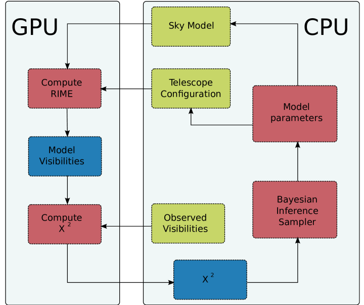
As discussed in the previous section, neither MeqTrees or OSKAR support evaluating the entire RIME on GPU, nor do they provide the facility to calculate a $\chi^{2}$ value. As BIRO makes many RIME evaluations, it is important to support this iterative approach to computation of the $\chi^{2}$. For this reason, Montblanc computes the entire RIME and $\chi^{2}$ on the GPU (Figure 3). The sky model, telescope configuration and observed visibilities are transferred to the GPU on each iteration and a single, floating point $\chi^{2}$ is transferred off. Data transfer to the GPU is overlapped by GPU kernel execution for a sufficient number of sources (See Section 4.4).

4.1 Data and ordering

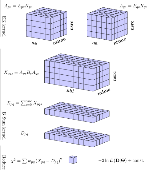
The input for the RIME (Table 2) is a series of 1D, 2D and 3D arrays, of which some are obtained from a CASA Measurement Set (MS) file (McMullin et al., 2007; Tran and Winkler, 2014). A workflow (Figure 4) is applied to solve the RIME and compute the $\chi^{2}$ value (the second normalization constant term is a function of the weight vector only and trivially calculated on the CPU via equation 10).

Firstly, the arrays are combined to create per-antenna values. The strategy here is to perform computationally expensive operations per-antenna, rather than per-baseline which is quadratically-greater in number.

The per-antenna terms are combined to create a 4D source-coherency array, followed by reduction to a 3D model visibility array. The model visibilities are subtracted from the data, squared, and multiplied by the weight vector, then summed to produced a single scalar $\chi^{2}$ value. Each of the 4D arrays’ values and 3D reductions can be computed independently.

In general, we order our GPU arrays by $\mathtt{ntime\times nbl\times nsrc\times nchan}$ where ntime and nchan are the slowest and most rapidly changing dimensions respectively. ntime and nbl are chosen as the first and second dimensions since the ordering of data in a CASA measurement set (MS) MAIN table is usually $\mathtt{ntime\times nbl}$. Using the same ordering as the MS avoids overly complex transpose operations and allows for efficient streaming from disk. In support of this, our CUDA kernels are 3D kernels with grid sizes of $\mathtt{ntime\times na\times nchan}$ and $\mathtt{ntime\times nbl\times nchan}$.

Each kernel loops over the source dimension. This is useful because the computation for point and Gaussian sources is different, making parallelisation over the source dimension unwieldy. New source types can be supported by adding another source loop to the kernel. Looping also increases the amount of work performed by each kernel thread, amortising the cost of kernel launch and clean-up (NVIDIA Corporation, 2014a). A 3D kernel configuration facilitates loading of per-timestep, -antenna and -channel data into shared memory at the start of the kernel. At each source-loop iteration, these data are combined with source data to form a tensor product. As each thread is accessing the same or similar source data simultaneously, this data will be retained in L1/L2 cache, increasing the opportunity for cache hits to occur.

Furthermore, the channel dimension is the easiest to parallelise since it is a 1D array and the same operation can be computed simultaneously for different wavelengths. This exploits CUDA’s SIMD architecture: each value is independent, leading to coalesced reads and writes to global memory.

Kernel	Registers	Threads per Block	Occupancy
EK float	31	512	87%
EK double	44	256	59%
B Sum float	46	256	60%
B Sum double	63	128	50%

Table 3: Kernel Configuration. This table shows the number of registers, threads per block and the occupancy of each kernel, as reported by the NVIDIA Profiler (NVIDIA Corporation, 2013).

procedure EKKernel(time $\mathtt{t}$,antenna $\mathtt{p}$,channel $\mathtt{\lambda}$)

     Read uvw coordinates and wavelengths from RAM into shared memory.

     for all point sources $s$ do

         Read lm coordinates into shared memory.

         Synchronize Threads

         Compute tensor $\mathtt{K[t,p,s,\lambda]}$

         Compute tensor $\mathtt{E[t,p,s,\lambda]}$

         Compute $\mathtt{A[t,p,s,\lambda]=E[t,p,s,\lambda]\times K[t,p,s,\lambda]}$

         Write $\mathtt{A[t,p,s,\lambda]}$ to DRAM.

         Synchronize Threads

     end for

     for all Gaussian sources $s$ do

         Read lm coordinates into shared memory.

         Synchronize Threads

         Compute tensor $\mathtt{K[t,p,s,\lambda]}$

         Compute tensor $\mathtt{E[t,p,s,\lambda]}$

         Compute $\mathtt{A[t,p,s,\lambda]=E[t,p,s,\lambda]\times K[t,p,s,\lambda]}$

         Write $\mathtt{A[t,p,s,\lambda]}$ to DRAM

         Synchronize Threads

     end for

end procedure

Algorithm 1 The EK kernel is parallelised over time, antennas and channel dimensions. Each source type is handled as a loop, in which the per-antenna value for each source is computed and outputted. Extending Montblanc to support $\beta$ profiles would involve adding a new loop to the kernel.

procedure BSumKernel(time $\mathtt{t}$,baseline $\mathtt{pq}$, channel $\mathtt{\lambda}$)

     $\mathtt{V[t,pq,\lambda]\leftarrow 0}$

     Read uvw coordinates and wavelengths from DRAM into shared memory.

     for all $s$ in point sources do

         Read $\mathtt{B[t,s]}$ into shared memory.

         Synchronize Threads

         Read $\mathtt{A[t,p,s,\lambda]}$ and $\mathtt{A[t,q,s,\lambda]}$ from DRAM

         $\mathtt{X[t,pq,\lambda,s]=A[t,p,s,\lambda]\times B[t,s]\times A[t,p,s,\lambda].H}$

         $\mathtt{V[t,pq,\lambda]+=X[t,pq,\lambda,s]}$

         Synchronize Threads

     end for

     for all $s$ in gaussian sources do

         Read $\mathtt{B[t,s]}$ into shared memory.

         Synchronize Threads

         Read $\mathtt{A[t,p,s,\lambda]}$ and $\mathtt{A[t,q,s,\lambda]}$ from DRAM

         $\mathtt{X[t,pq,\lambda,s]=A[t,p,s,\lambda]\times B[t,s]\times A[t,p,s,\lambda].H}$

         $\mathtt{V[t,pq,\lambda]+=X[t,pq,\lambda,s]}$

         Synchronize Threads

     end for

     Output $\mathtt{V[t,pq,\lambda]}$ to DRAM $\triangleright$ Optional

     Read $\mathtt{w[t,pq,\lambda]}$, $\mathtt{D[t,pq,\lambda]}$ from DRAM

     Output $\mathtt{w[t,pq,\lambda]\times\left(V[t,pq,\lambda]-D[t,pq,\lambda]\right)^{2}\equiv\chi^{2}[t,pq,\lambda]}$ to DRAM

end procedure

Algorithm 2 The B sum kernel is parallelised over time, baseline and channel. The visibility is initialised and a loop is employed for each source type. Within each loop, the appropriate per-antenna values for the baseline are read, and combined with the source brightness matrix to form a source coherency. These are added to the visibilities. Once the model visibilities have been calculated, they are differenced with the observed visibilities to calculate a $\chi^{2}_{pq}$ term for each visibility.

(a) EK kernel.

(b) B sum kernel.

Figure 5: Arithmetic Intensities of the EK and B Sum kernel, for a given number of point and Gaussian sources.

Figure 6: A roofline model of multiple GPU architectures, as well as that of 2 hexacore Xeon E5–2620 v2 CPUs. This model provides a theoretical estimate of an algorithm’s attainable GFLOPS/s, given it’s arithmetic intensity, on different computing architectures. The numbers shown for these devices are only attainable through the use of fused multiply adds (FMA) on data in registers. Generally, kernels consist of a much wider range of instructions and memory types, and therefore their peak performance is correspondingly lower. For example the dashed blue line illustates a more realistic performance pattern. Kernels with low arithmetic intensity cannot approach a device’s maximum performance, or roof, and are classified as memory bound. They must wait for data in order to exercise the processor, By contrast, high arithmetic intensity algorithms do approach the roof by executing many instructions, and are classified as compute bound. The point at which the arithmetic intensity changes from memory to compute bound is the balance zone. This occurs at approximately 14 FLOPS/byte for Kepler devices and 3.93 FLOPS/byte for the Xeons. This model suggests that the two kernels are memory bound on Keplers, with arithmetic intensity of 1.75 and 10 FLOPS/byte respectively. However, these kernels are composed of more general instructions and in practice, their balance zone would occur at lower arithmetic intensity. Determing the compute or memory bound nature of these kernels is accomplished through profiling.

4.2 Kernels for computing the BIRO RIME solution

Calculating the RIME is accomplished through three CUDA kernels. The number of registers, threads per block and occupancy for the first two are shown in Table 3.

(i) The EK kernel (Algorithm 1) computes per-antenna terms, $\mathtt{A[t,p,s,\lambda]}$, using the analytic expressions in Equations 5 and 6. It is parallelised over the ntime, na and nchan dimensions and loops over the nsrc dimension. A complex scalar $\mathtt{A[t,p,s,\lambda]=E[t,p,s,\lambda]\times K[t,p,s,\lambda]}$ is generated for each source and the resulting $\mathtt{ntime\times na\times nsrc\times nchan}$ array is written to the GPU’s global memory for use by the B sum kernel (see below). In practice, this kernel is inexpensive compared to others and therefore contains the computationally expensive trigonometric and transcendental functions of the RIME.

(ii) The B sum kernel (Algorithm 2) combines the $\mathtt{A[t,p,s,\lambda]}$ terms produced by the EK kernel, along with a source brightness matrix $\mathtt{B[t,s]}$, to form per-baseline source coherencies $\mathtt{X[t,pq,\lambda,s]}$. It is parallelised over the ntime, nbl and nchan dimensions and also loops over the nsrc dimension. Internally, the loop computes source coherencies and sums them to produce a $\mathtt{ntime\times nbl\times nchan}$ array of model visibilities $\mathtt{V[t,pq,\lambda]}$. The model visibilities are then subtracted from the observed visibilities $\mathtt{D[t,pq,\lambda]}$, squared and multiplied with the weight vector $\mathtt{w[t,pq,\lambda]}$ to produce a $\mathtt{ntime\times nbl\times nchan}$ array of $\chi^{2}$ terms. This kernel is the most expensive since the space of values it must process is of size $\mathtt{ntime\times nbl\times nsrc\times nchan}$. It is not entirely necessary to write the visibilities to the GPU’s global memory at this point, but this functionality allows Montblanc to act as a simulator.

(iii) The final reduction kernel is a standard reduction (Harris, 2005; Harris et al., 2007) of the $\chi^{2}_{pq}$ terms to produce a single $\chi^{2}$ value from which the likelihood $\mathcal{L}\left(\mathbf{D}|\mathbf{\Theta}\right)$ can be trivially calculated on the CPU using equation 10.

4.3 Kernel Analysis

Operation	float	double
EK Kernel
Instruction	68%	75%
Memory	15%	35%
B Sum Kernel
Instruction	65%	62%
Memory	35%	45%

Table 4: The NVIDIA profiler’s (NVIDIA Corporation, 2013) estimate of the percentage of time spent executing instructions and memory loads. The profiler considers the EK kernel to be compute bound, while it considers the B sum kernel to be balanced: neither compute nor memory bound.

Operations	bandwidth	% of	bandwidth	% of
	GB/s (float)	peak	GB/s (double)	peak
Shared Loads	398.424	-	334.269	-
Shared Stores	147.775	-	139.231	-
Global Loads	132.189	-	205.546	-
Global Stores	2.758	-	4.298	-
L1/Shared Total	681.147	$\approx$ 30%	683.344	$\approx$ 20%
L2 Cache Total	134.987	$\approx$ 30%	209.844	$\approx$ 40%
Device Memory Total	8.108	$\approx$ 10%	12.619	$\approx$ 10%

Table 5: Memory Performance of the B sum kernel as reported by the NVIDIA Profiler (NVIDIA Corporation, 2013). Global Loads/Stores are reads from DRAM, or global memory, while Shared Loads/Stores are reads from shared memory. These four figures are totalled under L1/Shared. Global operations are grouped with L1 cache because they go through the L1 cache in Fermi devices. This is not the case for Kepler devices. Global operations do go through the L2 cache for both architectures and the sum of Global Loads/Stores equals the L2 Cache total. The utilisation of L1 and L2 cache is high relative to DRAM, or Device Memory. This indicates many cache hits, resulting in the avoidance of expensive DRAM requests.

We have analysed the arithmetic intensity of the EK and B Sum kernels, estimating the number of FLOPS for the sinf (14), cosf (14), sincosf (14), expf (11) and powf (54) functions based on the __internal_accurate functions in CUDA’s math_functions.h header file. Note that many of these instructions are composed of FMA’s to approximate Taylor series for example. As the kernels loops through sources, the FLOPs and byte reads are dependent on the number of point (P) and Gaussian (G) sources. We analysed each kernel, line by line, to determine these counts and found that they are governed by the following expressions:

EK arithmetic intensity $$=\frac{6+127(P+G)}{4(6+3(P+G))}$$ (13)

B sum arithmetic intensity $$=\frac{73+57P+77G}{4(17+8P+11G)}$$ (14)

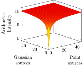
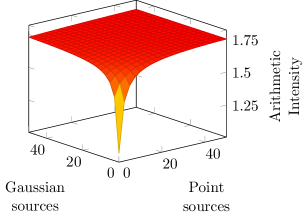
Figure 5 shows how this intensity varies for a given number of sources. It can be seen that the arithmetic intensity of the EK kernel is $\approx 10$, while that of the B sum kernel is $\approx 1.75$ and these numbers hold for varying numbers of point and Gaussians sources. In practice, these values will be higher since each block and thread accesses the same values for each source, resulting in L1 and L2 cache hits.

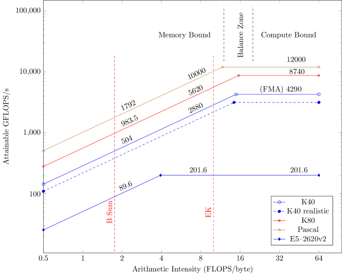
It is useful to plot the arithmetic intensity of these kernels on a Roofline Model (Figure 6). This model relates the theoretical peak performance of an algorithm in GFLOPS/s for different compute architectures, given it’s arithmetic intensity. The K40 and dual hexacore Xeons have a theoretical maximum, or roof, of 4290 and 201.6 GFLOPS/s respectively, and a maximum memory bandwidth of 288 GB/s and 51.2 GB/s respectively. The disadvantage of the dual Xeon architecture, compared to the GPUs is clearly visible in the model: A Xeon Phi 5110P with memory bandwidth of 320 GB/s and 60 cores would be more competitive. The trend for CPU and GPU architectures to increase in both performance and memory bandwidth continues. The values plotted at the intersection arithmetic intensity and GFLOPS/s show projected performance.

Compute bound algorithms have high arithmetic intensity and are ideal in the sense that they are bound by the device’s peak performance. At 10 FLOPS/byte, the EK kernel approaches this limit. By contrast, the B Sum kernel is memory bound at 1.75 FLOPS/byte. Such algorithms have low arithmetic intensity and, being more dependent on memory reads, do not fully exercise a device’s compute capabilities. The point at which an algorithm becomes less dependent on data and more constrained by instruction execution, occurs between compute and memory bound kernels in the balance zone. For example, this zone occurs at $3.93$ FLOPS/byte for Xeons and $\approx 14$ FLOPS/byte for Kepler devices

In practice, this performance only occurs for FMA instructions operating on data in registers. More general algorithms have difficulty fully exercising a device’s compute and memory bandwidth. This means that the balance zone actually occurs in areas of lower arithmetic intensity. To discover the compute or memory bound nature of the kernels, we used the NVIDIA profiler and recorded the results in Table 4. The profiler considers the EK kernel to be compute bound, spending most of it’s time executing intructions. This agrees with the kernel’s high arithmetic intensity rating. However, the B sum kernel spends comparitively more time on memory loads. The profiler considers it to be balanced – neither compute nor memory bound. This is surprising considering it’s relatively low arithmetic intensity. To see why this is the case, we must examine how the K40’s cache responds to the kernel (Table 5).

For loads, the ratio of L1 and L2 cache bandwidth to device memory, or DRAM bandwidth is high, $(334.269+205.546)/12.619=42.7\times$ in the double precision case. This behaviour occurs because, parallelised over multiple timesteps, baselines and frequencies, we loop over sources $s$, synchronising all threads. Therefore, all SMX’s handle one source in parallel and consequently, a small portion of the brightness array is simultaneously available in L2 cache to all SMX’s. e.g. $\mathtt{B[t,6]}$ for point source 6. Additionally, other data such as uvw coordinates and wavelength is also stored in shared memory (L1 cache). Retaining significnat portions of the problem in cache means that many slower trips to DRAM can be avoided: the caching capabilities of Kepler have hidden the memory bound nature of the B sum kernel, making it appear balanced.

We also investigated using Kepler’s L1 read cache to store source and per-antenna data, but did not find a significant performance difference with our current approach.

4.4 Scaling the RIME

Figure 7: Asynchronous Overlap of Data Transfer and Kernel Execution. This figure shows the computation of three separate solutions to the RIME for 100 sources. Computation tends to completely overlap data transfer when the number of sources $\simeq 75$.

⬇

import montblanc

# Obtain a solver

with montblanc.get_biro_solver(’WSRT.MS’,version=’v3’,

npsrc=10,ngsrc=10,dtype=numpy.float32) as slvr:

# Register a UVW array of floating point values

slvr.register_array(name=’uvw’,

shape=(3,’ntime’,’nbl’), dtype=’ft’)

# Transfer some random UVW coordinates to the GPU

slvr.transfer_uvw(np.random.random(

shape=slvr.uvw_shape, dtype=slvr.uvw_dtype))

# Register a property

slvr.register_property(name=’ref_wave’,

dtype=’ft’,default=1.4e9,value=1.4e9)

# Set the property

slvr.set_ref_wave(0.2)

slvr.solve() # Solve the BIRO RIME

print slvr.X2 # Print the Chi-squared value

Algorithm 3 Sample Montblanc code. A solver is obtained that loads the interferometer configuration from the WSRT.MS measurement set, and specifies 10 point and gaussian sources and single floating-point precision. A uvw array is registered on the solver and random (by way of illustration) uvw coordinates transferred to the GPU. A reference wavelength property is also registered on the solver. Thereafter, the RIME is solved and the $\chi^{2}$ value is retrieved from the solver object.

If the dimensions involved in the RIME are small enough, the required data may be small enough to fit into the memory of a single GPU. In practice, this will not be the case, considering how these dimensions scale for forthcoming interferometers: for example, MeerKAT will have 64 antennas, 2016 baselines and 32,000 channels, while the SKA will have $\approx 3600$ antennas, $\approx 6.5$ million baselines and 256,000 channels. Solving the RIME for the SKA instrument may require highly specialised or new computing architectures. However, it is possible to subdivide the RIME into parts that can be solved within the memory budgets on contemporary hardware architectures.

As the values of the RIME terms can be calculated independently, computation of the RIME can be divided so that the problem fits within the memory budget of a single GPU, individual components can be solved on multiple GPUs or even multiple GPUs on physically separate computers.

Here, the $\mathtt{ntime\times(nbl|na)\times nsrc\times nchan}$ ordering chosen for Montblanc’s imposed on our arrays is important since each input, temporary and output array adheres to it . Additionally, each array is registered in a manner similar to a numpy array, with an array shape and type. Montblanc takes this further by allowing strings naming each dimension to be used in addition to integer shape parameters. See the register_array method in Algorithm 3 for example.

Once the problem size is known, string parameters are replaced with integer dimensions and the amount of memory required for each array and the total problem is derived. Then, if the problem is too large to fit into a supplied memory budget, the problem is subdivided along the time dimension. For example, if a problem of size $\mathtt{ntime\times nbl\times nsrc\times nchan}$ cannot fit into a GPU memory, but $\mathtt{4\times nbl\times nsrc\times nchan}$ can, then two solvers handling problems of size $\mathtt{2\times nbl\times nsrc\times nchan}$ are created which solves for a $\chi^{2}$ over 2 timesteps, all baselines, sources and channels. Then, we iterate over timesteps, transferring data related to those timesteps into solvers. Each solver solves it’s part of the $\chi^{2}$ and the result is added together to a $\chi^{2}$ total on the CPU. By allocating two solvers, we take advantage of CUDA’s asynchronous architecture: The data required for one solver can be transferred to the GPU asynchronously while the other solver is performing computation. As the input (3D) and output (1 scalar) are smaller relative to the amount of computation (4D), the BIRO RIME is again well-suited to GPU implementation. Through empirical tests we have observed that the latency incurred by data transfer is fully overlapped by execution when $\simeq 75$ sources are specified (See Figure 7). Consequently we categorise the RIME as Dependent-Streaming according to the taxonomy of Gregg and Hazelwood (2011).

At present, subdividing along the time dimension suffices for problem sizes posed by current telescopes, such as Westerbork and LOFAR. However, newer telescopes will have more baselines and channels, increasing their sensitivity. They will therefore be able to detect fainter sources, increasing the number of sources in BIRO’s sky models.

However, the subdivision strategy described above can simply be extended down the row-major ordering. For example, if it is not possible to fit all timesteps and baselines into a GPU memory, solvers can be allocated catering for a problem size of $\mathtt{1\times 2\times nsrc\times nchan}$: each solver now solves one timestep, two baselines, all sources and all channels. However, increasing subdivision means that the problem size is outstripping the parallelism afforded by a single GPU.

Thus, increasing time, channel and source dimensions pose a computational challenge to solving the RIME. One mitigating factor is the continually increasing computing power and memory of modern GPUs. A K80 Kepler features 24GB of RAM over a K40’s 12GB, and the newer NVIDIA Pascal architectures will feature $\pm$ 12000 GFLOP/s, compared to the K40’s 4290 GFLOPS/s.

The obvious solution is to utilise multiple GPU and clustered solutions to the to recover some parallelism. Properly considered, this raises interesting questions as to whether it is even feasible to store the observed visibilities in a Measurement Set file. Instead, it may be necessary to stream these visibilities directly off a telescope into the RIME solver. We intend to explore these directions in future work.

One other possible avenue is to take an information theoretic approach and examine which RIME inputs actually contribute to the $\chi^{2}$ value. Certain channels, baselines and sources may have negligble impact. It remains to be seen whether discarding information negatively impacts the Bayesian inference process.

4.5 Implementation Details

Montblanc was developed in Python, using the numpy (Oliphant et al., 2014; van der Walt et al., 2011) and PyCUDA (Klöckner et al., 2012) packages, and is publicly available at
https://github.com/ska-sa/montblanc under a GPL2 license.

The architecture is designed to be highly modular and extensible. A contributor Rivi (2015) has already added Sersic profiles Sérsic (1963) for example. The basis for the architecture is a Solver object, on which the arrays used to solve the RIME are registered. Registering an array automatically creates numpy arrays on the CPU and CUDA arrays on the host, as well as transfer functions for moving data from the CPU arrays to GPU arrays. Scalar properties can also be registered on the solver. A simple usage pattern is demonstrated in Algorithm 3.

Developers are not restricted to using the Montblanc RIME for BIRO. The Solver executes a pipeline of GPU kernels which can be flexibly configured to suit a particular use case. Such kernels are represented as Python string templates, allowing a developer to embed string constants into the kernel.

Montblanc supports both single- and double-precision kernels. This is useful since single-precision floating-point accuracy will degrade once RIME dimensions scale upwards, especially in kernel sums and reductions. It may be possible to employ Kahan sums to reduce this (Kahan, 1965). The RIME computed by the GPU kernels is unit tested against CPU numpy (Oliphant et al., 2014) code, accelerated with the numexpr library (Cooke et al., 2014).

5 Results

We tested our code on a high-performance computer configured with a dual Intel Xeon(R) hexacore E5–2620v2 3.00GHz CPU, 128GB of memory and a NVIDIA K40 Tesla card.

Antennas	Baselines	Montblanc (s)	OSKAR (s)	Ratio	MeqTrees (s)	Ratio
float
7	21	0.0042	0.3980	93.51	–	–
14	91	0.0136	0.4314	31.67	–	–
27	351	0.0435	0.6246	14.33	–	–
64	2016	0.2320	1.7840	7.69	–	–
128	8128	0.7007	5.8305	8.32	–	–
192	18336	1.5730	12.4372	7.90	–	–
double
7	21	0.0073	0.4504	61.28	1.8183	247.39
14	91	0.0215	0.6164	28.62	5.5171	256.13
27	351	0.0703	1.1169	15.87	17.3753	246.94
64	2016	0.3668	4.5315	12.35	96.0943	261.98
128	8128	0.9113	16.8675	18.51	–	–
192	18336	2.3540	37.4096	15.89	–	–

Table 6: Timings for different problem sizes. This table shows the time taken to compute the RIME for varying numbers of antennas and baselines, as well as the speedup that Montblanc achieves vs OSKAR and MeqTrees. 64 channels, 100 timesteps, 50 point and 50 Gaussian sources were used in all cases.

(a) Single precision.

(b) Double precision.

Figure 8: Single and double-precision kernel running times for different baseline sizes. The B Sum kernel dominates computational cost as the number of antennas, and by implication, baselines increase.

5.1 Kernel running times and computational complexity

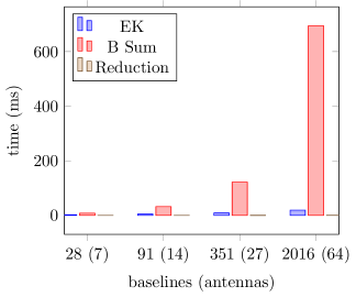
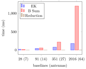
The running times for our kernels are shown in Figure 8 for different baselines. With a computational complexity of $O(\textrm{log}_{2}(\mathtt{ntime\times nbl\times nchan}))$, the reduction kernel contributes minimally to computational cost. By contrast, the B Sum kernel consumes most of the cost once the number of baselines starts to scale. This is because the computational complexity of the different kernels differ: $O(\mathtt{ntime\times na\times nsrc\times nchan})$ and $O(\mathtt{ntime\times nbl\times nsrc\times nchan})$ for the EK and B Sum kernels respectively. Due to the quadratic relation between the number of baselines and the number of antennas, the B Sum kernel will, in general, consume quadratically more time. Therefore, Montblanc takes on the computational complexity of the B Sum kernel, i.e. $O(\mathtt{ntime\times nbl\times nsrc\times nchan})$.

These figures support our decision to separate expensive, per-antenna computation into the EK kernel while assigning the multiplication and summation steps to the B Sum kernel: increasing the expense of the dominant complexity factor is a poor design choice. For example, the EK kernel is slower for the 7-antenna double-precision case, but the B Sum kernel rapidly outstrips it on the 64-antenna case.

Folding EK and B Sum kernels into a monolothic kernel operating over the ntime, na and nchan dimensions is an interesting proposition: the EK kernel’s compute capabilities could be used to hide the latency of the B sum kernel even further by computation of expensive per-antenna values. These values could be output to DRAM, and then multiplied and summed based on a triangular number pattern. However, this is not currently possible due to CUDA’s lack of block-level synchronisation.

Additionally, combining both the calculation, multiplication and sum of per-antenna terms into a monolithic kernel increases register usage and decreases occupancy. The double-precision B sum kernel already uses 63 registers and has a 50% occupancy. Further reductions in occupancy would reduce the solution’s parallelism.

5.2 Comparison with OSKAR

(a) OSKAR.

(b) MeqTrees.

Figure 9: The ratio, or speedup, of Montblanc’s GPU implementation on a NVIDIA K40 Kepler versus MeqTrees and OSKAR’s RIME implementation for varying antenna numbers. MeqTrees executed on a dual hexacore E5–2620v2 system, while OSKAR executed on the K40. 64 channels, 100 timesteps, 50 point and 50 Gaussian sources were used in all cases.

We performed a performance comparison between Montblanc and OSKAR’s interferometer simulator. OSKAR supports parts of the RIME on the CPU and the GPU. In the OSKAR output below, it can be seen that horizon clipping and the Jones E term, both implemented on the CPU, together consume almost 80% of simulation time.

=|== Simulation completed in 16.345 sec. | |  2.6% Chunk copy & initialise. | 69.1% Horizon clip. |  6.3% Jones R. | 10.3% Jones E. |  0.4% Jones K. |  1.0% Jones join. |  5.5% Jones correlate. | | + Writing Measurement Set: ’VLA27.MS’ |=|== Run complete.

Figure 10: Rime Dimension Variation. This graph shows the effect of varying each RIME dimension on the execution time. Adding timesteps and channels is twice as expensive as adding sources.

Therefore in our comparison, we have chosen to compare only those parts of the RIME that are present on the GPU, namely the Jones K kernel, Jones join kernel and the Jones correlate kernel. Thus we estimated OSKAR’s performance for the above case as follows: $16.345s\times(0.4\%+1.0\%+5.5\%)=1.127805s$.

Note that Montblanc’s GPU timing includes both a E term, computation of the $\chi^{2}$ terms and reduction to a single $\chi^{2}$ value. Montblanc’s E term is however, simpler than OSKAR’s. As such, it is difficult to perform a direct comparison, but the supplied figures provide an indication of relative performance.

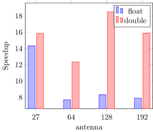
Table 6 and Figure 9a show that Montblanc is much faster than OSKAR for smaller antenna numbers, but this advantage drops when the number of antennas (and baselines) is large. In these cases Montblanc is at least 7.7 and 12 times faster than OSKAR for single and double-precision floating point respectively.

5.3 Comparison with MeqTrees

We performed a comparison of Montblanc’s GPU implementation with MeqTrees. However, the maximum theoretical performance of the B Sum kernel on the dual Xeon system is lower than on the K40. If the B Sum kernel, which dominates the computation for large problem sizes, were to be implemented on the CPU, it would, at most be able to achieve $1.75\times 51.2=89.6$ GFLOPS/s. This is 44% of the Xeon’s theoretical peak performance, and $5.625$ times less than the kernel’s theoretical peak of $504$ GFLOPS/s on the K40 (Figure 6.

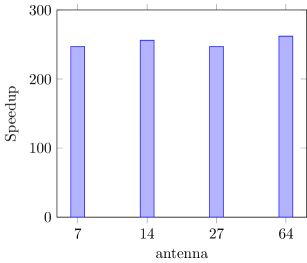
The speed-ups achieved are shown in Figure 9b. Channels, timesteps, point and Gaussian sources were held constant at dimensions of 64, 100, 50 and 50 respectively. The number of antennas was varied between 7, 14, 27 and 64, corresponding to the KAT7, Westerbork, VLA and MeerKAT telescopes. MeqTrees was configured to use all 12 cores available to the system. It can be seen that Montblanc is around 250X faster than MeqTrees, due to the disparity between CPU and GPU architectures.

5.4 RIME Dimension Variation

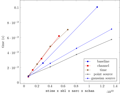
We performed analysis of our RIME solution to investigate the expense of increasing each dimension. This involved varying each dimension from a base configuration of 7 baselines, 64 channels, 100 timesteps, 50 point sources and 50 Gaussian sources. Figure 10 shows the total number of elements, $\mathtt{ntime\times nbl\times nsrc\times nchan}$ versus the time taken to solve the RIME.

It can be seen that increases in each dimension result in linear performance scaling. The numbers of timesteps and channels contribute most to the expense of the solution, followed by the baseline dimension. Gaussian and point sources are the least expensive dimensions to increase – roughly half as expensive as timesteps and channels. Point sources are marginally less expensive than Gaussians.

We expect that the ntime and nsrc dimensions will vary most for different problems, since channels and baselines will likely remain static for individual interferometers.

6 Conclusion

In this paper we presented Montblanc, a GPU-accelerated framework for solving the RIME in order to accelerate the BIRO technique. Using NVIDIA’s CUDA architecture, it computes the RIME and differences the resulting model visibilities with those observed by an interferometer to produce multiple $\chi^{2}$ likelihood values. These values are used to drive the Bayesian inference process.

At present, it supports point and Gaussian sources, time-varying source brightness and both single and double-precision solutions. It is architected to allow addition of other source morphologies, such as $\beta$ profiles and the computation can be subdivided in order to fit large problem sizes within a single GPUs memory. While only single GPUs are currently supported, this subdivision makes multi-GPU and clustered solutions to the RIME viable.

Expensive, per-antenna terms are computed in an EK kernel, and output to the GPU’s main memory. These per-antenna terms are read in by a B Sum kernel, and combined to form per-baseline terms. Model visibilities are computed from these terms and a $\chi^{2}$ value that is used by BIRO in the Bayesian inference process.

We have analysed our CUDA kernels, showing that one kernel dominates the run-time. Theoretical analysis suggests that the arithmetic intensity of this kernel is 1.75 FLOPS/byte, indicating a memory bound algorithm. By contrast, profiling indicates a balanced kernel that is neither compute nor memory bound. This is due to the fact that much of the problem is retained in Kepler’s L1 and L2 cache, avoiding expensive trips to the GPU DRAM. The computational complexity of Montblanc is $O(\mathtt{ntime\times nbl\times nsrc\times nchan})$.

We compared Montblanc’s performance on an NVIDIA K40 Kepler GPU with MeqTrees execution on a dual hexacore E5–2620v2 Xeon system. For a problem size of 64 antennas, 100 timesteps, 64 channels, 50 point and 50 Gaussian sources, Montblanc is around 250 times faster. We also compared it against parts of the OSKAR simulator’s CUDA RIME pipeline, and found that it was at least 7.7 and 12 times faster for single and double-precision floating point cases, respectively.

Montblanc is implemented as a Python package, and is designed for the addition of new source profiles. It is not limited to use for BIRO; it computes visibilities and can be used as a fast simulator. Users may implement their own RIME implementation with a custom pipeline, if required. With the future addition of more general DIE and DDE matrices, it could also be used as a calibrator.

6.1 Future Work

As BIRO currently operates on fully calibrated data, it was not immediately necessary to include evaluation of the $G_{ps}$ (DIE) matrices. Additionally, analytic expressions were substituted for the $E_{ps}$ (DDE) terms. In future work, we intend to provide full support for these terms as matrices. In the case of the DIE matrices, this will allow Montblanc to perform sky modeling and calibration simultaneously.

The high parallelism inherent in the calculation of the BIRO RIME and $\chi^{2}$ calculation also make the problem amenable to subdivision. We aim to provide support for multiple GPUs and distribution of the computation amongst multiple High Performance Computing nodes. This will necessarily involve implementing an out-of-core solution for BIRO, and providing solutions for the data-transfer bottlenecks inherent to this solution.

7 Acknowledgments

The authors wish to acknowledge the following for their support and advice:
  •  Marzia Rivi for corrections to the manuscript.
  •  Stefan van der Walt for numpy and numexpr advice.
  •  Bruce Merry and Ben Hugo for CUDA/PyCUDA conversations.
  •  Michael Clark from NVIDIA.
  •  Andrew Lewis and Tim Carr for help compiling on hex.
  •  Computations were performed using facilities provided by the University of Cape Town’s ICTS High Performance Computing team: http://hpc.uct.ac.za
  •  Simon Perkins acknowledges SKA South Africa for a postdoctoral research fellowship.
  •  Jonathan Zwart acknowledges SKA South Africa for a postdoctoral research fellowship.
  •  Iniyan Natarajan acknowledges the HPC for Radio Astronomy Programme.
  •  Oleg Smirnov’s research is supported by the South African Research Chairs Initiative of the Department of Science and Technology and National Research Foundation.

References

- Alted (2010) Alted, F., 2010. Why modern cpus are starving and what can be done about it. Computing in Science and Engineering 12 (2), 68–71.
-
Barsdell et al. (2010)
Barsdell, B. R., Barnes, D. G., Fluke, C. J., 2010. Analysing astronomy
algorithms for graphics processing units and beyond. Monthly Notices of the
Royal Astronomical Society 408 (3), 1936–1944.
URL http://mnras.oxfordjournals.org/content/408/3/1936.abstract - Cooke et al. (2014) Cooke, D., Hochberg, T., Alted, F., et al., 2014. Numexpr 2.4. https://github.com/pydata/numexpr.
- Cornwell et al. (2008) Cornwell, T. J., Golap, K., Bhatnagar, S., Nov. 2008. The Noncoplanar Baselines Effect in Radio Interferometry: The W-Projection Algorithm. IEEE Journal of Selected Topics in Signal Processing 2, 647–657.
E. Bertin and S. Arnouts (1996)
E. Bertin, S. Arnouts, 1996. Sextractor: Software for source extraction.
Astronomy and Astrophysics Supplement Series 117 (2), 393–404.
URL http://www.astromatic.net/software/sextractor - Feroz et al. (2009a) Feroz, F., Hobson, M. P., Bridges, M., Oct. 2009a. MULTINEST: an efficient and robust Bayesian inference tool for cosmology and particle physics. Monthly Notices of the Royal Astronomical Society 398, 1601–1614.
- Feroz et al. (2009b) Feroz, F., Hobson, M. P., Zwart, J. T. L., Saunders, R. D. E., Grainge, K. J. B., Oct. 2009b. Bayesian modelling of clusters of galaxies from multifrequency-pointed Sunyaev-Zel’dovich observations. Monthly Notices of the Royal Astronomical Society 398, 2049–2060.
- Flynn (1972) Flynn, M., Sept 1972. Some computer organizations and their effectiveness. Computers, IEEE Transactions on C-21 (9), 948–960.
Gregg and Hazelwood (2011)
Gregg, C., Hazelwood, K., 2011. Where is the Data? Why You Cannot Debate
CPU vs. GPU Performance Without the Answer. In: Proceedings of the IEEE
International Symposium on Performance Analysis of Systems and Software.
ISPASS ’11. IEEE Computer Society, Washington, DC, USA, pp. 134–144.
URL http://dx.doi.org/10.1109/ISPASS.2011.5762730 -
Hamaker et al. (1996)
Hamaker, J. P., Bregman, J. D., Sault, R. J., 1996. Understanding radio
polarimetry. I. Mathematical foundations . Astron. Astrophys. Suppl. Ser.
117 (1), 137–147.
URL http://dx.doi.org/10.1051/aas:1996146 -
Harris (2005)
Harris, M., 2005. Mapping computational concepts to gpus. In: ACM SIGGRAPH
2005 Courses. SIGGRAPH ’05. ACM, New York, NY, USA.
URL http://doi.acm.org/10.1145/1198555.1198768 - Harris et al. (2007) Harris, M., et al., 2007. Optimizing parallel reduction in CUDA. NVIDIA Developer Technology 2 (4).
Hobson and Maisinger (2002)
Hobson, M. P., Maisinger, K., 2002. Maximum-likelihood estimation of the cosmic
microwave background power spectrum from interferometer observations. Monthly
Notices of the Royal Astronomical Society 334 (3), 569–588.
URL http://mnras.oxfordjournals.org/content/334/3/569.abstract - Högbom (1974) Högbom, J. A., Jun. 1974. Aperture Synthesis with a Non-Regular Distribution of Interferometer Baselines. Astronomy and Astrophysics Supplement 15, 417.
Kahan (1965)
Kahan, W., Jan. 1965. Pracniques: Further remarks on reducing truncation
errors. Commun. ACM 8 (1), 40–.
URL http://doi.acm.org/10.1145/363707.363723 - Kazemi et al. (2011) Kazemi, S., Yatawatta, S., Zaroubi, S., Lampropoulos, P., de Bruyn, A. G., Koopmans, L. V. E., Noordam, J., Jun. 2011. Radio interferometric calibration using the SAGE algorithm. MNRAS414, 1656–1666.
- King (1966) King, I. R., Feb. 1966. The structure of star clusters. III. Some simple dynamical models. A J71, 64.
- King (1972) King, I. R., Jun. 1972. Density Data and Emission Measure for a Model of the Coma Cluster. ApJ Lett.174, L123.
- Klöckner et al. (2012) Klöckner, A., Pinto, N., Lee, Y., Catanzaro, B., Ivanov, P., Fasih, A., 2012. PyCUDA and PyOpenCL: A Scripting-Based Approach to GPU Run-Time Code Generation. Parallel Computing 38 (3), 157–174.
- Levenberg (1944) Levenberg, K., 1944. A method for the solution of certain non-linear problems. The Quarterly Journal of Applied Mathematics 2, 164–168.
Lochner et al. (2015)
Lochner, M., Natarajan, I., Zwart, J. T. L., Smirnov, O., Bassett, B. A.,
Oozeer, N., Kunz, M., 2015. Bayesian inference for radio observations.
Monthly Notices of the Royal Astronomical Society 450 (2), 1308–1319.
URL http://mnras.oxfordjournals.org/content/450/2/1308.abstract - MacKay (2003) MacKay, D. J. C., 2003. Information Theory, Inference, and Learning Algorithms. Cambridge University Press.
- Marquardt (1963) Marquardt, D., 1963. An algorithm for least-squares estimation of nonlinear parameters. The Quarterly Journal of Applied Mathematics 11 (2), 431–441.
- McMullin et al. (2007) McMullin, J. P., Waters, B., Schiebel, D., Young, W., Golap, K., 2007. Astronomical Data Analysis Software and Systems XVI (ASP Conf. Ser. 376), ed. RA Shaw, F. Hill, & DJ Bell (San Francisco, CA: ASP) 127.
- Mohan and Rafferty (2015) Mohan, N., Rafferty, D., Feb. 2015. PyBDSM: Python Blob Detection and Source Measurement. Astrophysics Source Code Library, record acsl1502.007.
- Moore (1965) Moore, G., 1965. Cramming More Components onto Integrated Circuits. Electronics 38 (4).
- Mort et al. (2010) Mort, B. J., Dulwich, F., Salvini, S., Zarb Adami, K., Jones, M. E., Oct 2010. Oskar: Simulating digital beamforming for the ska aperture array. In: Phased Array Systems and Technology (ARRAY), 2010 IEEE International Symposium on. pp. 690–694.
- Navarro et al. (1997) Navarro, J. F., Frenk, C. S., White, S. D. M., Dec. 1997. A Universal Density Profile from Hierarchical Clustering. Astrophys. J.490, 493–+.
Noordam and Smirnov (2010)
Noordam, J. E., Smirnov, O. M., 2010. The meqtrees software system and its
use for third-generation calibration of radio interferometers. Astronomy and
Astrophysics 524, A61.
URL http://dx.doi.org/10.1051/0004-6361/201015013 - NVIDIA Corporation (2013) NVIDIA Corporation, 2013. Profiler User’s Guide. NVIDIA Corporation.
- NVIDIA Corporation (2014a) NVIDIA Corporation, 2014a. CUDA C Programming Guide. NVIDIA Corporation.
- NVIDIA Corporation (2014b) NVIDIA Corporation, 2014b. Whitepaper: NVIDIA’s Next Generation CUDA Compute Architecture: Kepler GK110. http://www.nvidia.com/content/PDF/kepler/NVIDIA-kepler-GK110-Architecture-Whitepaper.pdf.
- Oliphant et al. (2014) Oliphant, T., et al., 2014. Numpy 1.9.1. https://github.com/numpy/numpy.
Popping and Braun (2008)
Popping, A., Braun, R., 2008. The standing wave phenomenon in radio
telescopes - Frequency modulation of the WSRT primary beam. Astronomy and
Astrophysics 479 (3), 903–913.
URL http://dx.doi.org/10.1051/0004-6361:20079122 - Rivi (2015) Rivi, M., January 2015. Commit https://github.com/ska-sa/montblanc/commit/bafa4b6 merged in pull request https://github.com/ska-sa/montblanc/pull/68.
- Sérsic (1963) Sérsic, J. L., 1963. Influence of the atmospheric and instrumental dispersion on the brightness distribution in a galaxy. Boletin de la Asociacion Argentina de Astronomia La Plata Argentina 6, 41.
Smirnov (2011a)
Smirnov, O. M., 2011a. Revisiting the radio interferometer
measurement equation - I. A full-sky Jones formalism. Astronomy and
Astrophysics 527, A106.
URL http://dx.doi.org/10.1051/0004-6361/201016082 -
Smirnov (2011b)
Smirnov, O. M., 2011b. Revisiting the radio interferometer
measurement equation - II. Calibration and direction-dependent effects.
Astronomy and Astrophysics 527, A107.
URL http://dx.doi.org/10.1051/0004-6361/201116434 - Thompson et al. (2007) Thompson, A. R., Moran, J. M., Swenson, G. W. J., May 2007. Interferometry and synthesis in radio astronomy. Wiley-Interscience.
- Tran and Winkler (2014) Tran, Q.-N., Winkler, F., 2014. Casa reference manual (version february 7, 2014).
- van der Walt et al. (2011) van der Walt, S., Colbert, S. C., Varoquaux, G., March 2011. The numpy array: A structure for efficient numerical computation. Computing in Science Engineering 13 (2), 22–30.