A scattering model of 1D quantum wire regular polygons

Abstract

We calculate the quantum states of regular polygons made of 1D quantum wires treating each polygon vertex as a scatterer. The vertex scattering matrix is analytically obtained from the model of a circular bend of a given angle of a 2D nanowire. In the single mode limit the spectrum is classified in doublets of vanishing circulation, twofold split by the small vertex reflection, and singlets with circulation degeneracy. Simple analytic expressions of the energy eigenvalues are given. It is shown how each polygon is characterized by a specific spectrum.

C. Estarellas and L. Serra

1 Introduction

Nanowires are a long-lasting topic of interest in nanoscience for two main reasons. One is, undoubtedly, their use as electron waveguides in devices and technological applications. The other is the possibility of using nanowires to artificially control quantum properties at the nanoscale, thus improving our fundamental understanding and prediction capabilities. In nanowires made with 2D electron gases of semiconductors like GaAs quantum behavior manifests at a mesoscopic scale, beyond the atomistic description, and it can be described with effective mass models and smooth potentials [1, 2].

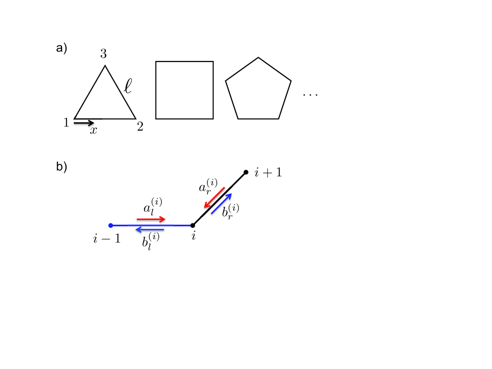
Figure 1: a) Sketch of the regular polygons made of 1D nanowires. The vertex labeling and the definition of a longitudinal coordinate $x$ is indicated only for the triangle. b) Scattering amplitudes as defined for a given vertex $i$.

The quantum states on nanowire bends attracted much interest some years ago [3, 4, 5, 6, 7, 8, 9, 10]. It was shown that bound states form on the bend, and the transmission and reflection properties as a function of the energy and width of the wire were thoroughly investigated. In the single-mode limit of a 2D wire a bend can be described with an effective 1D model containing an energy-dependent potential [6]. In the case of a circular bend, the situation becomes simpler and analytical approximations using a square well whose depth and length are fixed by the radius and angle of the bend were suggested [5].

Motivated by the above mentioned interest on nanowire bends we study in this work polygonal structures made of 1D quantum wires (Fig. 1). We focus on the single-mode limit and describe each vertex as a scatterer. The vertex scattering matrix is taken from the model of circular bends in 2D nanowires. We find that the spectrum fully characterizes the polygon structure. Two kinds of states are present: a) doublets, with a small energy splitting due to reflection and with a vanishing circulation along the perimeter of the polygon; and b) singlets, with an underlying degeneracy by which the circulation can take arbitrary values within a given range. The energy splitting of the doublets depends on the reflection probability of the vertex, while the number of singlets between consecutive doublets (in energy) can be used to infer the number of vertices. The energy scale, setting the separation between states, is fixed by the length of the nanowire forming the sides of the polygon.

We finally remark that, although our approach is on physical modeling of nanostructures, there is a connection with the more mathematically oriented study of quantum graphs [11]. Indeed, from this perspective our results can be viewed as a particular application to the case of regular polygons of the more general question of reconstructing the graph topology from the knowledge of the spectrum.

2 Theoretical model and method

We consider a regular polygon with $N_{v}$ vertices, made of 1D quantum wires of length $\ell$ (Fig. 1). The distance along the perimeter is measured by variable $x$, with origin arbitrarily taken on the first vertex. The wave function between vertices $i$ and $i+1$ is a superposition of left- and right-ward propagating plane waves

$$\psi(x) = a_{r}^{(i)}e^{-ip(x-x_{i})}+b_{r}^{(i)}e^{ip(x-x_{i})}$$ (1)

$$= a_{l}^{(i+1)}e^{ip(x-x_{i+1})}+b_{l}^{(i+1)}e^{-ip(x-x_{i+1})}\;,$$

where the first and second equalities take the reference point on vertices $i$ and $i+1$, respectively. The $a^{(i)}_{l/r}$ and $b^{(i)}_{l/r}$ coefficients are the characteristic input and output scattering amplitudes defined in Fig. 1b. We are assuming a single propagating mode of wavenumber $p$ (see A) and the set of vertex positions is $\{x_{i},i=1,\dots,N_{v}\}$.

The $i$-th vertex scattering equation relates output and input amplitudes as

$$\left(\begin{array}[]{c}b_{l}^{(i)}\\ \rule{0.0pt}{14.22636pt}b_{r}^{(i)}\end{array}\right)=\left(\begin{array}[]{cc}r&t\\ t&r\end{array}\right)\left(\begin{array}[]{c}a_{l}^{(i)}\\ \rule{0.0pt}{14.22636pt}a_{r}^{(i)}\end{array}\right)\;,$$ (2)

where $t$ and $r$ are the usual transmission and reflection complex coefficients. The scattering matrix in Eq. (2) is summarizing the physical effect of the vertex by means of two complex quantities, $t$ and $r$. As they are required inputs in our model, we will take these values from the known scattering matrices of circular bends in 2D nanowires. Actually, as discussed in A, in the single-mode limit there is an analytical description of the scattering by a circular bend in terms of an effective square well depending on the radius and angle of the bend [5].

There is a relation between input and output amplitudes of successive vertices,

$$b_{l}^{(i)} = a_{r}^{(i-1)}e^{-ip\ell}\;,$$ (3)

$$b_{r}^{(i)} = a_{l}^{(i+1)}e^{-ip\ell}\;.$$ (4)

The phase $e^{-ip\ell}$ in Eqs. (3) and (4) appears due to the assumption of two different reference points when considering the scattering processes from two consecutive vertices.

We define the circulation

$${\cal C}\equiv\frac{\hbar p}{m}\left(\left|a_{l}^{(i)}\right|^{2}-\left|b_{l}^{(i)}\right|^{2}\right)N_{v}\ell\;,$$ (5)

independent on the choice of vertex $i$ due to flux conservation. The circulation is also the same if one chooses the right coefficients ($a^{(i)}_{r}$ and $b^{(i)}_{r}$) instead of the left ones in Eq. (5). Physically, the circulation is measuring the probability current flowing along the polygon in a particular state, characterized by a set of $a$ and $b$ coefficients and a wave number $p$ (corresponding to an energy $E$).

In B we define an energy-dependent measure ${\cal F}(E)$, such that it vanishes for the eigenenergies of the polygon. In practice, we scan numerically the values of ${\cal F}(E)$ in order to determine the eigenenergies within a given energy interval.

3 Results

Figure 2 shows the energy dependence of ${\cal F}$ and ${\cal C}$ for polygonal structures from 3 to 6 vertices for a representative set of parameters. As mentioned above, the energies for which ${\cal F}$ vanishes are the physical eigenenergies of the polygon. We considered a representative energy interval above the threshold $\varepsilon_{1}=\hbar^{2}\pi^{2}/(2md^{2})$. The energy $\varepsilon_{1}$ corresponds to the first transverse mode of the 2D nanowire of width $d$ from which our 1D model derives (see A).

Figure 2: Energy dependence of the $\mathcal{F}$ measure in arbitrary units (black) and the circulation ${\cal C}$ in units of $\hbar p/m$ (gray-red). The unit of energy is $\hbar^{2}/md^{2}$. The wave number $p$ and the wire parameter $d$ are defined in Sec. 2. As indicated, each panel corresponds to a polygon with a different number of vertices $N_{v}$ but the same arm length $\ell=30d$. The figure shows the presence of doublets with vanishing circulation and singlets with maximal positive circulation ${\cal C}_{0}$. Notice that at the energies of the singlets the circulation can take values from $-{\cal C}_{0}$ to $+{\cal C}_{0}$. Other parameters: $R=1.3d$.

From Fig. 2 we notice that the polygon spectra are characterized by a sequence of doublets, with small energy splittings and with vanishing circulation ${\cal C}$. In addition to the doublets, there are a varying number of single-energy modes (singlets) with finite ${\cal C}$ lying in between doublets. For $N_{v}=3$, for instance, doublets around 5.02 and 5.13 with two intermediate singlets are seen in the upper left panel. Remarkably, doublets at the same energies are present in polygons with odd and even number of vertices. Polygons with an even number of vertices, however, possess additional doublets at intermediate energies.

Singlets in Fig. 2 are characterized by having ${\cal C}\approx N_{v}\hbar p/m\equiv{\cal C}_{0}$. Notice, however, that different values of the circulation are possible for each singlet energy. Indeed, with the algorithm of B we find that a positive circulation ${\cal C}_{0}$ is obtained if requiring $a_{l}^{(i)}=1$ (for an arbitrary $i$) and negative circulation $-{\cal C}_{0}$ if requiring $a_{r}^{(i)}=1$. This indicates that for each singlet the circulation can actually take any value within the range $-{\cal C}_{0}<{\cal C}<{\cal C}_{0}$ by adequately superposing the solutions for positive and negative circulations. We have explicitly checked this possibility from the numerical solutions. This behavior manifests the connection between the symmetry breaking and the ${\cal C}$-degeneracy of the singlets.

A qualitative difference is seen when comparing left and right panels of Fig. 2. Polygons with an odd number of vertices have $N_{v}-1$ singlets in between vanishing-circulation doublets, while polygons with an even number of vertices only have $N_{v}/2-1$. This explicitly shows that by knowing the spectrum one may characterize the polygonal structure. For instance, a spectrum consisting of a sequence of mode doublets with three intermediate singlets would correspond to an octagon.

For the spectra with an even number of intermediate singlets a confusion might arise between the polygons with $N_{v}$ and $2N_{v}$ vertices. For instance, both the triangle and the hexagon in Fig. 2 have two intermediate singlets. Still, one may differentiate the two situations with the discussion on doublets of next subsection. In essence, for odd-$N_{v}$ polygons all doublets are similar in that each polygon side contains an even number of half wavelengths. On the contrary, for even-$N_{v}$ polygons consecutive doublets alternate from an even to an odd number of half wavelengths. As shown below, this difference can be seen counting the number of density maxima on a side of the polygon.

3.1 Doublets

The states with vanishing circulation are characterized by having $|a|=|b|$ on each side of the polygon. Besides vanishing circulation, doublets have a density that remains invariant by a translation from one polygon side to the next one (Figs. 3 and 4). This happens because the scattering amplitudes of successive vertices fulfill either $a^{(i)}=a^{(i+1)}$ or $a^{(i)}=-a^{(i+1)}$. At the same time, for a given vertex the coefficients also fulfill $a_{l}=\pm a_{r}$. Therefore, these vanishing-circulation states can be classified in four types as summarized in Tab. 1.

Table 1 also gives the secular equation determining the wave number $p$ and the energy of the eigenmode for each type of mode. Notice that solutions of types I and III are associated to states with maximal density on each vertex, while types II and IV have minimal density on the vertex, cf. Figs. 3 and 4. The split pair forming a doublet are therefore composed by solutions of types (I,II) and (III,IV). It is also worth stressing that solutions of type III and IV are not allowed in polygons with an odd number of sides. The reason is most easily understood assuming $r\approx 0$ and $t\approx 1$. In this case, the secular equation for types III and IV simplifies to $e^{ipl}=-1$; that is $\ell=(2n+1)\lambda/2$ and an odd number of half wavelengths should fit in a polygon side. For odd values of $N_{v}$ this is not compatible with the additional condition that the full perimeter should contain and integer number $n^{\prime}$ of wavelengths, $N_{v}\ell=n^{\prime}\lambda$.

Table 1: Different types of modes in vanishing-circulation doublets. The pairs forming doublets are (I,II) and (III,IV).

type	left-right	successive vertices	equation
I	$a_{l}=a_{r}$	$a^{(i)}=a^{(i+1)}$	$t+r=e^{-ip\ell}$
II	$a_{l}=-a_{r}$	$a^{(i)}=a^{(i+1)}$	$t-r=e^{-ip\ell}$
III	$a_{l}=a_{r}$	$a^{(i)}=-a^{(i+1)}$	$t+r=-e^{-ip\ell}$
IV	$a_{l}=-a_{r}$	$a^{(i)}=-a^{(i+1)}$	$t-r=-e^{-ip\ell}$

Simple analytical approximations for the doublet splittings can be obtained from the secular equations in Tab. 1 assuming $t\approx 1$ and $r\approx r_{0}e^{i\phi}$. This leads to the conditions ($n=1,2,3\dots)$

$$\begin{array}[]{ll}p\ell=2n\pi\mp r_{0}\sin\phi\;,&({\rm I,II})\;,\\ p\ell=(2n+1)\pi\mp r_{0}\sin\phi\;,&({\rm III,IV})\;.\end{array}$$ (6)

For both kinds of pairs the splitting in wave numbers is $\Delta p=2r_{0}\sin\phi/\ell$, with an associated energy splitting $\Delta=(\hbar^{2}/m)p\Delta p$. Equation (6) clearly shows that in (I,II) doublets, the solution of type I decreases its energy due to reflection while that of type II increases, and analogously for (III,IV) doublets. We recall that type I and III solutions are those with a maximal density on each vertex. Finally, we notice that as the energy increases the reflection coefficient is reduced, and so the doublet splitting is also reduced, as hinted also in Fig. 2.

Summarizing, the energies of the zero-circulation doublets are approximately

$$E_{n\pm}=\varepsilon_{1}+\frac{\hbar^{2}\pi^{2}n^{2}}{2m\ell^{2}}\pm\Delta\;,\quad\!\!\!\!\!\left\{\begin{array}[]{l}n=1,2,3,\dots({\rm even}\,N_{v})\;,\\ n=2,4,6,\dots({\rm odd}\,N_{v})\;.\end{array}\right.$$ (7)

Physically, our result of Eq. (7) says that the arm length $\ell$ determines the separation between successive doublets, while the reflection properties of the vertex determine the splitting $\Delta$ of the pair forming a doublet.

3.2 Singlets

The most remarkable feature of singlets is that the density is not equivalent on different sides of the polygon. As mentioned above, for each singlet different solutions with circulation ranging from $-{\cal C}_{0}$ to $+{\cal C}_{0}$, where ${\cal C}_{0}\approx N_{v}\hbar p/m$, are possible. The intermediate panels of Figs. 3 (energies of 5.049 and 5.086) and in Fig 4 (5.042 and 5.097) show the densities corresponding to singlets for the triangle and square. Continuum and dashed lines are for states with maximal and vanishing circulation, respectively. We notice that for states with non vanishing ${\cal C}$, the density for positive and negative circulations coincide. For nonvanishing circulation the density does not vanish at any point, but oscillates around a finite mean value. In all singlets, different behaviors are seen on the sides of the polygon.

The singlet energies and their underlying ${\cal C}$-degeneracy can be easily understood in the limit of vanishing reflection. Indeed, when $r\approx 0$ and $t\approx 1$ the solutions to Eqs. (2) and (3) decouple for positive and negative circulations. The input coefficients for vertex $k$ read in this case

$$\begin{array}[]{cccc}a_{r}^{(k)}&=&\alpha e^{ip\ell(k-1)}\;,&({\cal C}<0)\;,\\ a_{l}^{(k)}&=&\beta e^{-ip\ell(k-1)}\;,&({\cal C}>0)\;,\end{array}$$ (8)

where $\alpha$ and $\beta$ are arbitrary independent constants that can be fixed by normalization. A maximal circulation state is obtained when either $\alpha$ or $\beta$ vanish. Arbitrary superpositions can be formed for $\alpha\neq 0$ and $\beta\neq 0$, including a vanishing circulation state for $\alpha=\beta$. The cyclic condition in Eq. (8), $e^{ip\ell N_{v}}=1$, leads to the energies

$$E_{n}=\varepsilon_{1}+\frac{\hbar^{2}\pi^{2}(2n)^{2}}{2m\ell^{2}N_{v}^{2}}\;,\quad(n=1,2,3,\dots)\;.$$ (9)

These energies coincide with a doublet condition [Eq. (7) for $\Delta=0$] each time $n$ is an integer number of times $N_{v}$. It can be easily verified that Eq. (9) implies that for odd-$N_{v}$ polygons there are $N_{v}-1$ singlets between two successive doublets and that for even-$N_{v}$ polygons there are $N_{v}/2-1$, in agreement with the results of Fig. 2

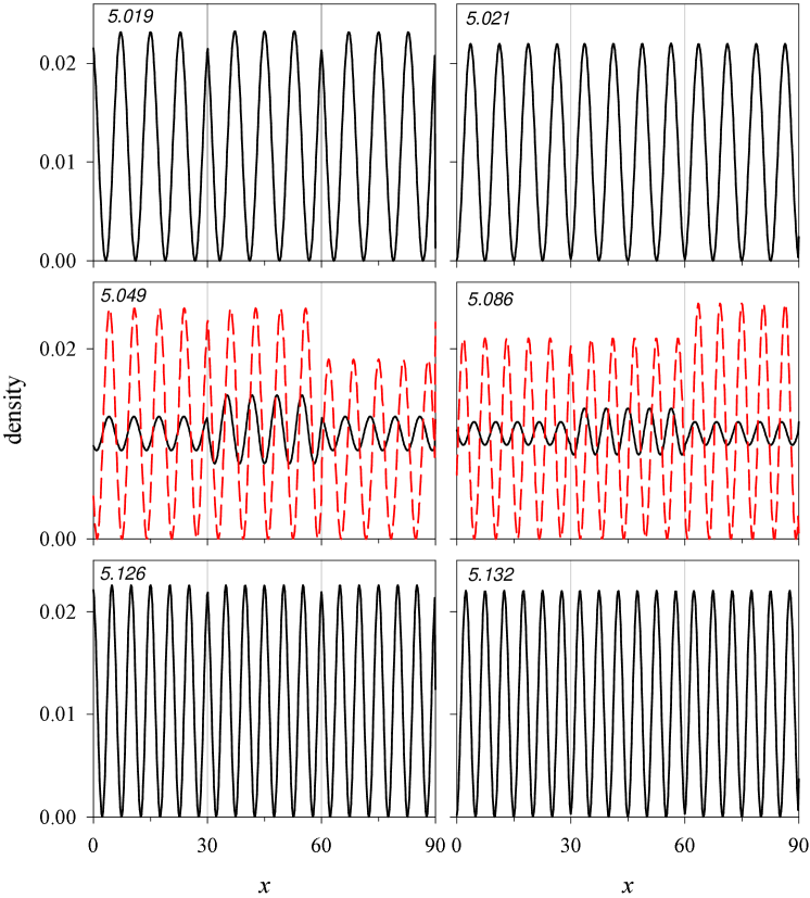
Figure 3: Densities for the triangle modes of Fig. 2. All distances are measured in units of $d$ (defined in A). Upper and lower panels are for vanishing-circulation doublets of type (I,II). Intermediate panels are singlets with maximal (solid) and vanishing (dashed) circulation. The energy of the mode (as in Fig. 2) is indicated in each panel. The position of vertices is given by the vertical lines. Rest of the parameters as in Fig. 2.

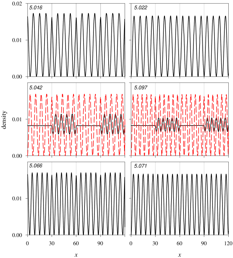
Figure 4: Same as Fig. 3 for the square modes. Upper panels are the first pair [type (I,II)], while lower panels are the second pair [type (III,IV)] in the results of Fig. 2 for the square. The two central panels are singlets with maximal (solid) and vanishing (dashed) circulation.

4 Conclusions

A model of closed polygons made of 1D quantum wires has been presented where each vertex is described as a scatterer. The vertex transmission and reflection coefficients have been described with the model of circular bends in 2D wires. The polygon spectra are characterized by a sequence of doublets, with a small energy splitting, and a typical number of singlets lying in between doublets. Odd-$N_{v}$ polygons have $N_{v}-1$ singlets while even $N_{v}$ have $N_{v}/2-1$ singlets in between two doublets. The doublet splittings are caused by the reflection on vertices. Doublets have a vanishing circulation and singlets can have circulations ranging from a negative to positive characteristic values. Approximate analytical expressions for the singlet and doublet energies have been given and the corresponding densities discussed. Our results explicitly show how the polygon characteristics can be inferred from the spectrum.

Appendix A Scattering by a 2D circular bend

We consider a 2D nanowire with a circular bend of angle $2\theta$ and radius $R$, as sketched in Fig. 5. Notice that $\theta$, defined as half the bend angle, is related in our model to the number of polygon vertices by $\theta=\pi/N_{v}$. The lateral extension of the nanowire is $d$, setting the energy of the first transverse mode to $\varepsilon_{1}=\hbar^{2}\pi^{2}/(2md^{2})$. Following Ref. [5], it is possible to derive an analytical expression for the reflection and transmission coefficients of the circular bend in the single-mode limit.

Defining $a=\bar{R}\theta$, where $\bar{R}=\sqrt{R(R+d)}$ is an average radius, the 2D scattering problem in the single mode limit is approximated by a 1D quantum well of width $2a$ and depth $V_{0}=-\hbar^{2}/(8m\bar{R}^{2})$. The analytical expressions of the $t$ and $r$ complex coefficients are given in terms of two wave numbers ($E>\varepsilon_{1}$)

$$p = \sqrt{\frac{2m}{\hbar^{2}}(E-\varepsilon_{1})}\;,$$ (10)

$$q = \sqrt{\frac{2m}{\hbar^{2}}(E-\varepsilon_{1}-V_{0})}\;.$$ (11)

Specifically, they read

$$t = \frac{4pq}{(p+q)^{2}e^{2i(p-q)a}-(p-q)^{2}e^{2i(p+q)a}}\;,$$ (12)

$$r = -\frac{2i(p-q)(p+q)\sin(2qa)}{(p+q)^{2}e^{2i(p-q)a}-(p-q)^{2}e^{2i(p+q)a}}\;.$$ (13)

Notice that, as expected, for large energies it is $p\approx q$ and Eqs. (12) and (13) then yield $t\approx 1$ and $r\approx 0$. We also stress that, due to symmetry, the transmission and reflection coefficients for left and right incidences are identical, $t^{\prime}=t$, $r^{\prime}=r$, leading to the scattering matrix of Eq. (2).

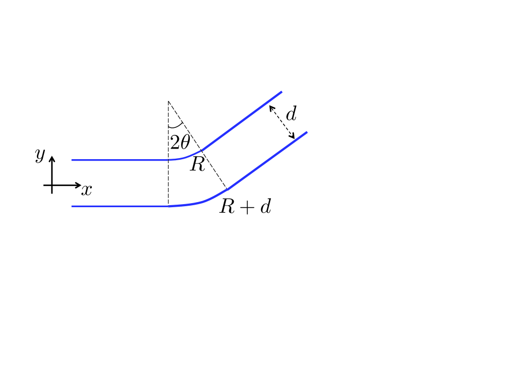
Figure 5: Circular bend in a 2D nanowire.

Appendix B Algorithm

Equations (2), (3) and (4) are set up as a homogoneous linear system

$${\mathbf{M}}\left(\begin{array}[]{c}{\mathbf{a}}\\ {\mathbf{b}}\end{array}\right)=0\;,$$ (14)

where we define the vector

$${\mathbf{a}}^{T}\equiv\left(a_{l}^{(1)}\dots a_{l}^{(N_{v})}a_{r}^{(1)}\dots a_{r}^{(N_{v})}\right)\;,$$ (15)

with an analogous definition for ${\mathbf{b}}$. Nontrivial solutions of Eq. (14) occur only for energies such that the determinant of ${\mathbf{M}}$ vanishes, ${\rm det}({\mathbf{M}})=0$.

In practice, we arbitrarily pick one of the components of ${\mathbf{a}}$, say $a_{\alpha}^{(\beta)}$, and fix it to 1, transforming Eq.  (14) into the inhomogeneous problem

$${\mathbf{M}}^{\prime}\left(\begin{array}[]{c}{\mathbf{a}}\\ {\mathbf{b}}\end{array}\right)={\mathbf{R}}\;,$$ (16)

where

$${\mathbf{R}}^{T}\equiv\left(0\dots 010\dots 0\dots 0\right),$$ (17)

with the value 1 on the position of the chosen component $a_{\alpha}^{(\beta)}$. Matrices ${\mathbf{M}}$ and ${\mathbf{M}}^{\prime}$ are identical except for the row of the chosen component, which is diagonal for ${\mathbf{M}}^{\prime}$. Equation (16) can be easily solved by standard numerical routines. The solution is then used to evaluate the following norm

$${\cal F}={\rm norm}\left\{{\mathbf{M}}\left(\begin{array}[]{c}{\mathbf{a}}\\ {\mathbf{b}}\end{array}\right)\right\}\;.$$ (18)

Obviously, when ${\cal F}=0$ the solution obtained from Eq. (16) is actually a solution of the original problem (14). The validity of the method is guaranteed by the linearity, for when a solution of (14) exists it can always be scaled such that a chosen component is equal to 1, provided only that it does not vanish. A simple energy scan of ${\cal F}$ will signal the position of the eigenenergies as the nodes of the function. We have checked that, as expected, the nodes are independent of the chosen component $a_{\alpha}^{(\beta)}$ and that they numerically coincide with the nodes of ${\rm det}({\mathbf{M}})=0$.

References

- [1] S. Datta, Electronic transport in mesoscopic systems, Cambridge University Press, 1997.
- [2] D. K. Ferry, G. S. M., B. Jonathan, Transport in nanostructures, Cambridge University Press, 2009.
- [3] C. S. Lent, Transmission through a bend in an electron waveguide, Appl. Phys. Lett. 56 (1990) 2554.
- [4] F. Sols, M. Macucci, Circular bends in electron waveguides, Phys. Rev. B 41 (1990) 11887–11891.
- [5] D. W. L. Sprung, H. Wu, J. Martorell, Understanding quantum wires with circular bends, J. Appl. Phys. 71 (1992) 515–517.
- [6] H. Wu, D. W. L. Sprung, J. Martorell, Effective one-dimensional square well for two-dimensional quantum wires, Phys. Rev. B 45 (1992) 11960–11967.
- [7] H. Wu, D. W. L. Sprung, J. Martorell, Electronic properties of a quantum wire with arbitrary bending angle, J. Appl. Phys. 72 (1992) 151–154.
- [8] H. Wu, D. W. L. Sprung, Theoretical study of multiple-bend quantum wires, Phys. Rev. B 47 (1993) 1500–1505.
- [9] K. Vacek, A. Okiji, H. Kasai, Multichannel ballistic magnetotransport through quantum wires with double circular bends, Phys. Rev. B 47 (1993) 3695–3705.
- [10] H. Xu, Ballistic transport in quantum channels modulated with double-bend structures, Phys. Rev. B 47 (1993) 9537–9544.
- [11] G. Berkolaiko, P. Kuchment, Introduction to quantum graphs, American Mathematical Society, 2012.