Complete Decentralized Method for On-Line Multi-Robot Trajectory Planning in Valid Infrastructures

Abstract

We consider a system consisting of multiple mobile robots in which the user can at any time issue relocation tasks ordering one of the robots to move from its current location to a given destination location. In this paper, we deal with the problem of finding a trajectory for each such relocation task that avoids collisions with other robots. The chosen robot plans its trajectory so as to avoid collision with other robots executing tasks that were issued earlier. We prove that if all possible destinations of the relocation tasks satisfy so-called valid infrastructure property, then this mechanism is guaranteed to always succeed and provide a trajectory for the robot that reaches the destination without colliding with any other robot. The time-complexity of the approach on a fixed space-time discretization is only quadratic in the number of robots. We demonstrate the applicability of the presented method on several real-world maps and compare its performance against a popular reactive approach that attempts to solve the collisions locally. Besides being dead-lock free, the presented approach generates trajectories that are significantly faster (up to 48% improvement) than the trajectories resulting from local collision avoidance.

Introduction

Consider a future factory where intermediate products are moved between workplaces by autonomous robots. The worker at a particular workplace calls a robot, puts an object to a basket mounted on the robot and orders the robot to autonomously deliver the object to another workspace where the object will be retrieved by a different worker. Clearly, an important requirement on such a system is that each robot must be able to avoid collisions with other robots autonomously operating in the shared space. The problem of avoiding collisions between individual robots can be approached either from a control engineering perspective by employing reactive collision avoidance or from AI perspective by planning coordinated trajectories for the robots.

In the reactive approach, the robot follows the shortest path to its current destination and attempts to resolve collision situations as they appear. Each robot periodically observes positions and velocities of other robots in its neighborhood. If there is a potential future collision, the robot attempts to avert the collision by adjusting its immediate heading and velocity. A number of methods have been proposed (?; ?; ?) that prescribe how to compute such collision-avoiding velocity in a reciprocal multi-robot setting, with the most prominent one being ORCA (?). These approaches are widely used in practice thanks to their computational efficiency – a collision-avoiding velocity for a robot can be computed in a fraction of a millisecond (?). However, these approaches resolve collisions only locally and thus they cannot guarantee that the resulting motion will be deadlock-free and that the robot will always reach its destination.

With a planning approach, the system first searches for a set of globally coordinated collision-free trajectories from the start position to the destination of each robot. After the planning has finished, the robots start following their respective trajectories. If robots are executing the resulting joint plan precisely (or within some predefined tolerance), it is guaranteed that the robots will reach their destination while avoiding collisions with other robots. It is however known that the problem of finding coordinated trajectories for a number of mobile objects from the given start configurations to the given goal configurations is intractable. More precisely, the coordination of disks amidst polygonal obstacles is NP-hard (?) and the coordination of rectangles in a bounded room is PSPACE-hard (?).

Even though the problem is relatively straightforward to formulate as a planning problem in the Cartesian product of the state spaces of the individual robots, the solutions can be very difficult to find using standard heuristic search techniques as the joint state-space grows exponentially with increasing number of robots. The complexity can be partly mitigated using techniques such as ID (?) or M* (?) that solve independent sub-conflicts separately, but each such sub-conflict can still be prohibitively large to solve because the time complexity of the planning is still exponential in the number of robots involved in the sub-conflict.

Instead, heuristic approaches are often used in practice, such as prioritized planning (?), where the robots are ordered into a sequence and plan one-by-one such that each robot avoids collisions with the higher-priority robots. This greedy approach tends to perform well in uncluttered environments, but it is in general incomplete and often fails in complex environments.

When the geometric constraints are ignored, complete polynomial algorithms can be designed such as Push&Rotate (?) or Bibox (?). These algorithms solve so-called “Pebble motion” problem, in which pebbles(robots) move on a given graph such that each pebble occupies exactly one vertex and no two pebbles can occupy the same vertex or travel on the same edge during one timestep. Although this model can be useful for coordination of identical robots on coarse graphs, it is not applicable for trajectory coordination of robots with fine-grained or otherwise rich motion models.

Recall that in our factory scenario, a robot can be assigned a task “online” at any time during the operation of the system. If one of the classical planners is used, the system would have to interrupt all the robots and replan their trajectories each time a new task is assigned, which is clearly undesirable. Further, although prioritized planning can be run in a decentralized manner (?; ?), the complete approaches are difficult to run without a central solver.

The main contribution of this paper is COBRA – a novel decentralized method for collision avoidance in multi-robot systems with online-assigned tasks to individual robots. We prove that for robots operating in environments that were designed as a valid infrastructures, the method is complete, i.e. all tasks are guaranteed to be successfully carried out without collision. Furthermore, if a time-extended roadmap planner is used for trajectory planning, the algorithm has polynomial worst-case time-complexity in the number of robots. The applicability of the approach is demonstrated using a simulated multi-robot system operating in real-world environments.

Problem Statement

Consider a 2-d environment (described by a set of obstacle-free coordinates $\mathcal{W}\subseteq\mathbb{R}^{2}$) and a set of points $E\subset\mathcal{W}$ representing distinguished locations in the environment called endpoints (modeling e.g. workplaces in a factory). The pair $(\mathcal{W},E)$ is called and infrastructure. Such an infrastructure is populated by $n$ mobile robots with circular bodies indexed $1,\ldots,n$. The radius of the body of robot $i$ is denoted $r_{i}$, the maximum speed robot $i$ can move at is denoted by $v_{i}^{\mathrm{max}}$. The robots are assumed to be holonomic, i.e. at every time step, the robot can select its immediate speed $v\in(0,v_{i}^{\mathrm{max}})$ and heading $\theta\in(-\pi,\pi)$ with the acceleration limits being neglected. During the operation of the system, robots are assigned relocation tasks denoted $s\rightarrow g$ requesting the chosen robot to move from its current position $s\in E$ to the given goal endpoint $g\in E$. We assume that the robot cannot be interrupted once it starts executing a particular relocation task and thus a new relocation task can be assigned to a robot only after it has reached the destination of the previously assigned task. The objective is to find a trajectory for each such relocation task such that the robot will reach the specified goal without colliding with other robots operating in the system. Moreover, such trajectories should be found in a decentralized fashion without a need for a central component coordinating individual robots.

Notation

In the remainder of the paper we will make use of the notion of a space-time region: When a spatial object, such as the body of a robot, follows a given trajectory, then it can be thought of as occupying a certain region in space-time $\mathcal{T}:=\mathcal{W}\times\left[0,\infty\right)$. A dynamic obstacle $\Delta$ is then a region in such a space-time $\mathcal{T}$. If $(x,y,t)\in\Delta$, then we know that the spatial position $(x,y)$ is occupied by dynamic obstacle $\Delta$ at time $t$. The function

$$R_{i}^{\Delta}(\pi):=\left\{(x,y,t):t\in[0,\infty)\wedge(x,y)\in R_{i}(\pi(t))\right\}$$

maps trajectories of a robot $i$ to regions of space-time that the robot $i$ occupies when its center point follows given trajectory $\pi$. As a special case, let $R_{i}^{\Delta}(\emptyset):=\emptyset$.

COBRA – General Scheme

In this section we will introduce Continuous Best-Response Approach (COBRA), a decentralized method for trajectory coordination in multi-robot systems. The general formulation of the algorithm assumes that each of the robots in the system is able to compute an optimal trajectory for itself from its current position to a given destination position in the presence of moving obstacles without prescribing how such a trajectory should be computed. In order to synchronize the information flow and ensure that the robots plan their trajectory using up-to-date information about the trajectories of others, robots are using a distributed token-passing mechanism (?) in which the token is used as a synchronized shared memory holding current trajectories of all robots. We identify a token $\Phi$ with a set $\{(a_{i},\pi_{i})\}$, which contains at most one tuple for each robot $a=1\ldots,n$. Each such tuple represents the fact that robot $a$ is moving along trajectory $\pi$. At any given time the token can be held by only one of the robots and only this robot can read and change its content.

A robot newly added to the system tries to obtain the token and to register itself with a trajectory that stays at its initial position forever.After all the robots have been added to the system, the user can start with assigning relocation tasks to individual robots.

When a new relocation task is received by robot $i$, the robot requests the token $\Phi$. When the token is obtained, the robot runs a trajectory planner to find a new “best-response” trajectory to fulfill the relocation task. The trajectory is required a) to start at the robot’s current position $p$ at time $t_{\mathrm{now}}+t_{\mathrm{planning}}$ (at the end of the planning window), b) to reach the goal position $g$ as soon as possible and remain at $g$ and c) to avoid collisions with all other robots following trajectories specified in the token. If such a trajectory is successfully found, the token is updated with the newly generated trajectory and released so that other robots can acquire it. Then, the robot starts following the found trajectory. Once the robot successfully reaches the destination, it can accept new relocation tasks. The pseudocode of the COBRA algorithm is listed in Algorithm 1.

1 On registered to the system at position $s$

2      

3      $\Phi\leftarrow$ request token ;

4      

5      $\pi\leftarrow$ $\pi(t)\text{ such that }\,\forall t\in[0,\infty):\;\pi(t)=s$ ;

6      

7      $\Phi\leftarrow$ $\Phi\cup\left\{(i,\pi)\right\}$ ;

8      

9      release token $\Phi$ ;

10      

11

12On new relocation task $s\rightarrow g$ assigned

13      

14      $\Phi\leftarrow$ request token ;

15      

16      assert $g$ is not a destination of another robot;

17      

18      $\Phi\leftarrow$ $\left(\Phi\setminus\left\{(i,\pi^{\prime})\,:\,(i,\pi^{\prime})\in\Phi\right\}\right)$ ;

19      

20      $\Delta\leftarrow\underset{(j,\pi_{j})\in\Phi}{\bigcup}R_{j}(\pi_{j})$;

21      

22      $t_{\mathrm{dep}}\leftarrow t_{\mathrm{now}}+t_{\mathrm{planning}}$ ;

23      

24      $\pi\leftarrow$ Best-traj_i($s$,$t_{\mathrm{dep}}$,$g$,$\Delta$) ;

25      

26      if $\pi=\emptyset$ then

27            

28            report failure

29      

30      $\Phi\leftarrow$ $\Phi\cup\left\{(i,\pi)\right\}$ ;

31      

32      release token $\Phi$ ;

33      

34      start following $\pi$ at $t_{\mathrm{dep}}$ ;

35      

36

37Function Best-traj_i($s$,$t_{s}$,$g$,$\Delta$)

38      

39      return trajectory $\pi$ for robot $i$ that reaches $g$ in minimal time such that

40       a) $\pi(t_{s})=s$,

41       b) $\exists t_{g}\,\forall t^{\prime}\in[t_{g},\infty):\>\pi(t^{\prime})=g$,

42       c) $R_{i}(\pi)\cap\Delta=0$ if it exists,

43      otherwise return $\emptyset$;

44      

45

Algorithm 1 COBRA – specification for robot $i$. The current time is denoted $t_{\mathrm{now}}$, the maximum time that can be spent in trajectory planning is denoted $t_{\mathrm{planning}}$.

Theoretical Analysis

In this section we will derive a sufficient condition under which is the presented mechanism complete, i.e. it guarantees that all relocation tasks will be successfully carried out without collision. First, observe that in general a robot may fail to find a collision-free trajectory to its destination as illustrated in Figure 1.

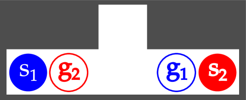
Figure 1: Scenario in which robot 2 fails to find a trajectory for a relocation task $s_{2}\rightarrow g_{2}$. First, robot 1 plans a trajectory for relocation task $s_{1}\rightarrow g_{1}$. It will travel at straight line connecting the two points at maximum speed. Robot 2 can travel at the same maximum speed as robot 1 and plans second from $s_{2}$ to $g_{2}$. However, it cannot reach the exchange point in time and thus none of the available trajectories reaches $g_{2}$ without collision with robot 1. The trajectory planning by robot 2 fails.

There is, however, a class of infrastructures, which we call valid infrastructures, where each trajectory planning is guaranteed to succeed and consequently all relocation tasks will be carried out without collision.

Informally, a valid infrastructure has its endpoints distributed in such a way that any robot standing on an endpoint cannot completely prevent other robots from moving between any other two endpoints. In a valid infrastructure, a robot is always able to find a collision-free trajectory to any other unoccupied endpoint by waiting for other robots to reach their destination endpoint, and then by following a path around the occupied endpoints, which is in a valid infrastructure guaranteed to exist.

In the following, we will describe the idea more formally. First, let us introduce the necessary notation. Let $D(x,r)$ be a closed disk centered at $x$ with radius $r$. Then, $\mathrm{int}_{r}\,X:=\left\{x:D(x,r)\subseteq X\right\}$ is an $r$-interior of a set $X\subseteq\mathbb{R}^{2}$ and $\mathrm{ext}_{r}\,X:=\underset{x\in X}{\cup}D(x,r)$ is an $r$-exterior of a set $X\in\mathbb{R}^{2}$. A path is a continuous function $p(\alpha):\,[0,1]\rightarrow\mathbb{R}^{2}$ which represents a curve in $\mathbb{R}^{2}$. A trajectory is a function $\pi(t):\,[0,\infty)\rightarrow\mathbb{R}^{2}$ which represents a movement of a point in $\mathbb{R}^{2}$ and time. Given a set $X\subseteq\mathbb{R}^{2}$, we say that a path $p$ is $X$-avoiding iff $\forall\alpha:\;p(\alpha)\notin X$. Similarly, a trajectory $\pi$ is $X$-avoiding iff $\forall t:\;\pi(t)\notin X$. The trajectories $\pi_{i}$ and $\pi_{j}$ of robots $i$ and $j$ are said to be collision-free iff $\forall t:\left|\pi_{i}(t)-\pi_{j}(t)\right|\geq r_{i}+r_{j}$. A trajectory $\pi$ is $g$-terminal iff $\exists t_{g}\,\forall t\in[t_{g},\infty):\;\pi(t)=g.$ Token $\Phi$ is called a) E-terminal iff $\forall(a,\pi)\in\Phi:\,\pi\text{ is }g\text{-terminal}$ and $g\in E$, and b) collision-free iff $\forall(a,\pi),\,(a^{\prime},\pi^{\prime})\in\Phi:\,a\neq a^{\prime}\Rightarrow\pi\text{ and }\pi^{\prime}\text{ are collision-free}.$

Definition 1.

An infrastructure $(\mathcal{W},E)$ is called valid for circular robots having body radii $r_{1},\ldots,r_{n}$ if any two endpoints $a,b\in E$ can be connected by a path in workspace $\mathrm{int}_{\overline{r}}\left(\mathcal{W}\setminus\underset{e\in E\setminus\{a,b\}}{\cup}D(e,\overline{r})\right)$, where $\overline{r}=\max\{r_{1},\ldots,r_{n}\}$.

In other words, there must exists a path between any two endpoints with at least $\overline{r}$-clearance with respect to the static obstacles and at least $2\overline{r}$-clearance to any other endpoint. Figure 2 illustrates the concept of a valid infrastructure.

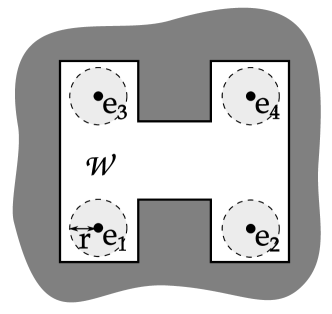
(a) Valid infrastructure: The workspace $\mathcal{W}$ and endpoints $\{e_{1},e_{2},e_{3},e_{4}\}$ for robots having radius $r$ form a valid infrastructure.

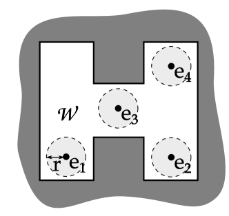
(b) Non-valid Infrastructure: The workspace $\mathcal{W}$ and endpoints $\{e_{1},e_{2},e_{3}\}$ do not form a valid infrastructure because there is no path from $e_{1}$ to $e_{2}$ with $2r$-clearance to $e_{3}$ for a robot having radius $r$.

Figure 2: Valid and non-valid infrastructure

The notion of valid infrastructures follows the structure typically witnessed in man-made environments that are intuitively designed to allow efficient transit of multiple people or vehicles. In such environments, the endpoint locations where people or vehicles are stopping for longer time are separated from the transit area that is reserved for travel between these locations.

If we take the road network as an example, the endpoints would be the parking places and the system of roads is built in such a way that any two parking places are reachable without crossing any other parking place. Similar structure can be witnessed in offices and factories. The endpoints would be all locations, where people may need to spend longer periods of time, e.g. surroundings of the work desks or machines. As we know from our every day experience, work desks and machines are typically given enough free room around them so that a person working at a desk or a machine does not obstruct people moving between other desks or machines. We can see that real-world environments are indeed often designed as valid infrastructures.

Completeness in Valid Infrastructures

In this section, we show that if robots are operating in a valid infrastructure and use COBRA for trajectory coordination, they will successfully carry out all assigned relocation tasks without collisions. Our analysis assumes the following setup of the multi-robot system. First, the robots must operate in a valid infrastructure $(\mathcal{W},E)$. When the system is initialized, robots are located at distinct initial endpoints of the infrastructure. After the initialization is finished, robots start accepting relocation tasks from some higher-level component, which ensures that each destination is an endpoint of the infrastructure and two robots will never have simultaneously assigned relocation task with the same destination. Each robot uses a complete trajectory planner and any trajectory generated for a robot, will be precisely followed by robot.

Proposition 2.

If token $\Phi$ acquired during handling of a new task $s\rightarrow g$ assigned to robot $i$ (on line 1 in Algorithm 1) is E-terminal and collision-free, then the subsequent trajectory planning succeeds and returns a trajectory that is $g$-terminal and collision-free with respect to other trajectories in $\Phi$.

Proof.

Because $(\mathcal{W},E)$ is a valid infrastructure and $s,g\in E$, there exists a $\mathrm{ext}_{r}\,\left(E\setminus\left\{s,g\right\}\right)$-avoiding path $p$ going from $s$ to $g$. All trajectories in $\Phi$ are E-terminal, which implies that eventually they reach one of the endpoints and stay at that endpoint. Consequently, there exists a time point $\overline{t}$ after which all the robots reach their destination endpoints and stay there. A $g$-terminal and collision-free trajectory for robot $i$ can be constructed as follows:

• In time interval $t\in[t_{s},\max(t_{s},\overline{t})]:\>\pi(t)=s$. The trajectory cannot be in collision with any other trajectory in $\Phi$ during this interval: From the assumption that new relocation tasks can be assigned only after the previous relocation task has been completed, we have $\forall t\in[t_{now},\infty):\,\pi(t)=g^{\prime}$. From the assumption that the start position of a new relocation task $s$ must be the same as the goal of the robots previous task $g^{\prime}$, we know $\forall t>t_{now}:\,\pi(t)=s$. Since $\Phi$ is collision-free, all trajectories of robots other than $j$ from $\Phi$ must be avoiding $s$ with $r_{i}+r_{j}$ clearance, where $r_{j}$ is the radius of the other robot in $\Phi$. Therefore, in time interval $[t_{s},\max(t_{s},\overline{t})]$, robot $i$ will be collision-free with respect to other trajectories stored in $\Phi$.

• In time interval $t\in[\overline{t},\infty]:\>$$\pi$ follows path $p$ until the goal position g is reached. The trajectory cannot be in collision with any trajectory in $\Phi$ during this interval: After time $\overline{t}$, all robots are at their respective goal positions $G$, which satisfy: a) $G\subseteq E$, b) $s\notin G$, otherwise some of the trajectories would have to be in collision with $\pi$, which contradicts the finding from the previous point, and c) $g\notin G$ because we assume that two robots cannot have simultaneously relocation tasks with the same destination. We know that the path $p$ avoids regions $\mathrm{ext}_{2\overline{r}}\,\left(E\setminus\left\{s,g\right\}\right)$ and thus the trajectory cannot be in collision with any other trajectory in $\Phi$ during the interval $[\overline{t},\infty)$.

Such a trajectory can always be constructed and thus any single-robot complete trajectory planning method must find it. ∎

Proposition 3.

Every time $\Phi$ is acquired by a robot during new relocation task handling (line 1 in Algorithm 1), $\Phi$ is E-terminal and collision-free.

Proof.

By induction on $\Phi$. Take an arbitrary sequence of individual robots acquiring the token $\Phi$ and updating it. Let the induction assumption be: Whenever $\Phi$ is acquired by a robot to handle a new relocation task, $\Phi$ is E-terminal and collision-free.

Base case: When the last robot registers itself, all robots have a trajectory in $\Phi$ that remains at their start positions forever. Since the start position are assumed to be distinct and at least $2\overline{r}$ apart, then the $\Phi$ is collision-avoiding. Further, $\Phi$ is trivially E-terminal because after the last robot registers, all robots stay at their initial position, which is an endpoint.

Inductive step: From the inductive assumption, we know that $\Phi$ acquired at line 1 in Algorithm 1 is E-terminal and collision-free. Using Proposition 2, we see that for any relocation task $s\rightarrow g$, the algorithm will find a trajectory $\pi$ that is g-terminal and collision-free with respect to other trajectories in $\Phi$. From our assumption, the destination $g\in E$. By adding trajectory $\pi$ to $\Phi$ at line 1 in Algorithm 1, the token $\Phi$ remains E-terminal and collision-free. ∎

Theorem 4.

If a team of robots operates in a valid infrastructure $(\mathcal{W},E)$ and the COBRA algorithm is used to coordinate relocation tasks between the endpoints of the infrastructure, then all relocation tasks will be successfully carried out without collision.

Proof.

By contradiction. Assume that a) there can be a relocation task $s\rightarrow g$ assigned to robot $i$ that is not carried out successfully or b) two robot collide at some time point during the operation of the system.

Case A: A relocation task $s\rightarrow g$ assigned to a robot $i$ has not been successfully completed. We assume that robots are able to perfectly follow any given trajectory $\pi$. Therefore either $\pi$ is not $g$-terminal or robot $i$ collided with another robot during the execution of the trajectory. From Proposition 2 and 3 we know that the Best-traj_i routine will always return a $g$-satisfactory trajectory. The possibility that the robot collided while carrying out a relocation task is covered by Case B and is shown to be impossible. Thus, the relocation task $s\rightarrow g$ assigned to robot $i$ will be completed successfully.

Case B: Robots $i$ and $j$ collide. Since we assume perfect execution of trajectories, it must be the case that there is $\pi_{i}$ and $\pi_{j}$ that are not collision-free. Since the collision relation is symmetrical, w.l.o.g., it can be assumed that $\pi_{j}$ was added to $\Phi$ later than $\pi_{i}$. This implies that $\pi_{i}$ was in the token $\Phi$ when $\pi_{j}$ was generated within Best-traj_j routine. However, this would imply that the trajectory planning returned a trajectory that is not collision-free with respect to trajectories in $\Phi$, which is a contradiction with constraints used during the trajectory planning. Thus, robots $i$ and $j$ do not collide.

We can see that neither case A nor case B can be achieved and thus all relocation tasks are carried out without any collision. ∎

COBRA with a Time-extended Roadmap Planner

In the previous section we have presented the general scheme of COBRA that assumes that every robot is able to find an optimal best-response trajectory for itself using an arbitrary complete algorithm. In practice, such a planning would be often done via graph search in a discretized representations of the static workspace. In this section, we will analyze the properties of COBRA when all robots use a roadmap-based planner to plan their best-response trajectory.

The function Best-traj_i($s$,$t_{s}$,$g$,$\Delta$) used on line 1 in Algorithm 1 returns an optimal trajectory for a particular robot $i$ from $s$ to $g$ starting at time $t_{s}$ that avoids space-time regions $\Delta$ occupied by other robots. We will now assume that the robots use a time-extended roadmap planner to compute such a trajectory. The planner takes a graph representation of the static workspace and extends it with a discretized time dimension. The resulting time-extended roadmap is subsequently searched using Dijkstra’s shortest-path algorithm (possibly with some admissible heuristic). The time-extended roadmap planner can be implemented as follows. Let us have a “roadmap” graph $G=(V,L)$ representing an arbitrary discretization of the static workspace $\mathcal{W}$, where $V\subseteq\mathcal{W}$ represent the discretized positions from $\mathcal{W}$ and $L\subseteq V\times V$ represents possible straight-line transitions between the vertices. The time-extended graph $\overline{G}=(\overline{V},\overline{L})$ for robot $i$ with time step $\delta t$ starting at position $s$ at time $t_{s}$ is recursively defined as follows:

$$(s,t_{s})\notin\Delta\Rightarrow(s,t_{s})\in\overline{V}$$ (1)

and

$$\forall(v,t)\in V\,\wedge\,(v_{1},v_{2})\in L:\,$$

$$t^{\prime}=\left\lceil\frac{\left|v_{2}-v_{1}\right|}{\delta t\cdot v_{i}^{max}}\right\rceil\delta t\,\wedge\mathrm{line}\left((v_{1},t),(v_{2},t^{\prime})\right)\cap\Delta=\emptyset$$ (2)

$$\Rightarrow$$

$$(v_{2},t^{\prime})\in\overline{V}\,\wedge\,\left((v_{1},t),(v_{2},t^{\prime})\right)\in\overline{L},$$

where $\left\lceil\cdot\right\rceil$ represents ceiling, $\left|\cdot\right|$ is the Euclidean norm, and $\mathrm{line(x,y)}$ represents the set of points lying on the line $x\rightarrow y$. It is important to realize that because we force each space-time edge to end a time that is a multiple of $\delta$t, some of the edges may in fact be traveled at a slower speed than $v_{i}^{\mathrm{max}}$. The best-response trajectory is then constructed by finding the shortest path in $\overline{G}$ starting from the vertex $(s,t_{s})$ to a goal vertex that satisfies $(g,t_{g})\,\wedge\,\mathrm{line\left((g,t_{g}),(g,\infty)\right)\cap\Delta=\emptyset}$.

Valid Infrastructure Roadmap

The notion of a valid infrastructure can be extended to discretized representations of the robots’ common workspace as follows.

Definition 5.

A graph $G=(V,L)$ is a roadmap for a valid infrastructure $(\mathcal{W},E)$ and robots with radii $r_{1},\ldots r_{n}$ if $E\subseteq V$ and any two different endpoints $a,b\in E$ can be connected by a path $p=l_{1},\ldots,l_{k}$ in graph $G$ such that

$$\underset{i=1,\ldots,k}{\forall}\mathrm{line(}l_{i})\subseteq\mathrm{int}_{\overline{r}}\left(\mathcal{W}\setminus\underset{e\in E\setminus\{a,b\}}{\cup}D(e,\overline{r})\right),$$

where $\overline{r}=\max\{r_{1},\ldots,r_{n}\}$.

Analogically to the valid infrastructure, we require that the roadmap contains a path that connects any two endpoints with at least $\overline{r}$ clearance to static obstacles and $2\overline{r}$ clearance to other endpoints.

Theoretical Analysis

In this section, we will show that COBRA with a time-extended roadmap planner operating on a roadmap for valid infrastructure is complete and the trajectory for any relocation task will be computed in time quadratic to the number of robots present in the system. In the following, we will assume that $G=(V,L)$ is a roadmap for a valid infrastructure $(\mathcal{W},E)$.

Theorem 6.

If $G=(V,L)$ is a roadmap for a valid infrastructure $(\mathcal{W},E)$ and COBRA with a time-extended roadmap planner is used to coordinate relocation tasks between the endpoints of the infrastructure, then all relocation tasks will be successfully carried out without collision.

Proof.

The line of argumentation used to prove the completeness of COBRA with an arbitrary complete trajectory planner (Theorem 4) is also applicable for COBRA with time-extended roadmap planner (TERP) – we only need to show that Proposition 2 holds when TERP is used to find the best-response trajectory. The original argument can be adapted as follows: If the robot acquires an E-terminal token, there is a time-point $\overline{t}$, when all robots in $\Phi$ reach their destinations and stay there. A best response trajectory for a relocation task $s\rightarrow g$ can always be constructed by waiting at the robot’s start endpoint until $\left\lceil\frac{\overline{t}}{\delta t}\right\rceil\delta t$ (the first discrete time-point, when all robots from $\Phi$ are on an endpoint) and then by following the shortest path from $s$ to $g$ on roadmap $G$. ∎

Complexity

In this section we derive the computational complexity of the COBRA algorithm when the time-extended roadmap planner is used for finding the best-response trajectory. We will focus on the complexity of trajectory planning for a single relocation task and show that if a robot acquires a token with trajectories of other robots, all the robots in the token will reach their respective destination endpoints in a relative time that is bounded by a factor linearly dependent on the number of robots. Therefore, the state space that needs to be searched during the trajectory planning is linear in the number of robots.

Assumptions and Notation: Let $f(\pi)$ denote the time when trajectory $\pi$ reaches its destination, i.e. $f(\pi):=\min\,t\,\text{s.t.}\,t^{\prime}\geq t:\,\pi(t^{\prime})=g,\>g\in E$. Further, let $A(\Phi,t)$ denote the set of “active” trajectories from token $\Phi$ at time $t$ defined as $A(\Phi,t):=\left\{\pi:(\cdot,\pi)\in\Phi\,\text{s.t. }f(\pi)\geq t\right\}$. The latest time when all trajectories in token $\Phi$ reach their destination endpoints is given by function $F(\Phi):=\underset{(\cdot,\pi)\in\Phi}{\max}f(\pi)$. Further, let $r$ denote the duration of the longest possible individually optimal trajectory between two endpoints by any of the robots: $$r=\underset{e_{1},e_{2}\in E}{\max}\frac{\text{length of shortest path from }e_{1}\text{ to }e_{2}\text{ in }G}{\underset{i=1\ldots n}{\min}v_{i}^{max}}.$$

Lemma 7.

At any time point $t$ we have $F(A(\Phi,t))\leq t+\left|A(\Phi,t)\right|r$.

Proof.

Observe that the token only changes during new task handling. Let us consider an arbitrary sequence of tasks being handled by different robots at time-point $\tau_{1},\tau_{2}\ldots$. Initially, at time $t=0$ the token is empty and the inequality holds trivially: $F(\emptyset)\leq 0$. We will inductively show that the inequality holds after the token update during each such task handling, which implies that it also holds for the time period until the next update of the token. Now, let us take $k^{\mathrm{th}}$-task handling by robot $i$ with current trajectory $\pi_{i}$, that at time $\tau^{k}$ obtains token $\Phi^{k-1}$. By induction hypothesis we have $F(A(\Phi^{k-1},\tau^{k}))\leq\tau^{k}+\left|A(\Phi^{k-1},\tau^{k})\right|r$. We know that $\pi_{i}\notin A(\Phi^{k-1},\tau^{k})$, because the robot can only accept new tasks after it has finished the previous one and thus $f(\pi_{i})<\tau^{k}$. Further, we know that 1) $\forall\pi\in\Phi^{k-1}\setminus A(\Phi^{k-1},\tau^{k})\;\forall t>\tau^{k}:\>\pi(t)\in E$ and 2) $\forall\pi\in A(\Phi^{k-1},\tau^{k})\;\forall t>F(A(\Phi^{k-1},\tau^{k}))\>\pi(t)\in E$, i.e. “inactive” trajectories are on the endpoints immediately, while active trajectories will reach their endpoints and stay there after $F(A(\Phi^{k-1},\tau^{k})$. Then, the robot finds its new trajectory $\pi_{i}^{\star}$, which can be in the worst-case constructed by waiting at the current endpoint and then following the shortest endpoint-avoiding path (which is in infrastructures guaranteed to exist and its duration is bounded by $r$) to the destination endpoint. Such a path reaches the destination in $\tau^{k}\leq f(\pi_{i}^{\star})\leq F(A(\Phi^{k-1},\tau^{k})+r$. Then, the robot updates token $\Phi^{k}\leftarrow\Phi^{k-1}\setminus\left\{\pi_{i}\right\}\cup\left\{\pi_{i}^{\star}\right\}$. We know that $\pi_{i}\notin A(\Phi^{k-1},\tau^{k})$, but $\pi_{i}^{\star}\in A(\Phi^{k},\tau^{k})$ and thus $\left|A(\Phi^{k},\tau^{k})\right|=\left|A(\Phi^{k-1},\tau^{k})\right|+1$. By rearrangement

$$\begin{aligned} F(A(\Phi^{k-1},\tau^{k}))&\leq\tau^{k}+\left|A(\Phi^{k-1},\tau^{k})\right|r\\ F(A(\Phi^{k},\tau^{k}))&\leq F(A(\Phi^{k-1},\tau^{k}))+r\\ F(A(\Phi^{k},\tau^{k}))&\leq\tau^{k}+\left|A(\Phi^{k-1},\tau^{k})\right|r+r\\ F(A(\Phi^{k},\tau^{k}))&\leq\tau^{k}+\left|A(\Phi^{k-1},\tau^{k})+1\right|r\\ F(A(\Phi^{k},\tau^{k}))&\leq\tau^{k}+\left|A(\Phi^{k},\tau^{k})\right|r\end{aligned}.$$

∎

Lemma 8.

During each relocation task handling of robot $i$ at time $t$, there is a trajectory $\pi$ that reaches the destination of the relocation task in time $f(\pi)\leq t+nr$.

Proof.

It is known that $F(A(\Phi,t))\leq t+\left|A(\Phi,t)\right|r$. Token $\Phi$ is updated in such a way that it contains at most one record for each robot. Assume that robot $i$ handles a new relocation task. Before planning, robot $i$ removes its trajectory from token $\Phi$ and thus we have $\left|\Phi\right|\leq n-1$. Since $\left|A(\Phi,t)\right|\subseteq\Phi$, we have $\left|A(\Phi,t)\right|\leq n-1$ and using Lemma 7, we get $F(A(\Phi,t))\leq t+(n-1)r$, i.e. all other robots will be at their respective destination endpoint at latest time $t+(n-1)r$. In the worst case, trajectory $\pi$ can be constructed by waiting at robot’s $i$ current endpoint until time $t+(n-1)r$ and then following the shortest path to its destination endpoint, which can take at most $r$. Trajectory $\pi$ thus reaches the destination endpoint latest at time $t+(n-1)r+r=t+nr$.∎

Theorem.

The worst-case asymptotic complexity of a single relocation task handling using COBRA with time-extended roadmap planning is $O(n^{2}v^{2}(\frac{1}{\delta t})^{2}r(d+r))$, where $n$ is the number of robots in the system, $v$ is the number of vertices in the roadmap graph, $\delta t$ is the time-discretization step, $r$ is the maximum duration of a single relocation when the interactions between robot are ignored, and $d$ is the duration of longest space-time edge in time-extended roadmap.

Proof.

Suppose that robot $i$ handles a relocation task $s\rightarrow g$. Let $v$ denote the number of vertices of the roadmap graph. In the worst case, the time-extended graph can contain all vertices from the roadmap $G$ for each time step. The best-response trajectory is the shortest path from the initial vertex $(s,t_{s})$, where $t_{s}=t+t_{\mathrm{planning}}$ to a goal vertex $(g,t_{g})$. The search algorithm will only need to examine the subgraph for the time interval $[t_{s},t_{g}]$, which contains at most $\left\lceil\frac{(t_{g}-t_{s})}{\delta t}\right\rceil v$ vertices. We know $t_{g}\leq t+nr$ (from Lemma 8) and $t_{s}>t$ (because $t_{s}=t+t_{\mathrm{planning}}$ and $t_{\mathrm{planning}}>0$) and thus this subgraph will have at most $\left\lceil\frac{nr}{\delta t}\right\rceil v\overset{\sim}{=}\frac{nrv}{\delta t}$ vertices for $\delta t\ll nr$. This graph first needs to be constructed and then searched. Construction: During the construction of the space-time subgraph for robot $i$, each edge $\epsilon$ has to be checked for collisions with moving obstacles $\Delta$ composed of $n$ space-time regions, each representing the disc body of another robot $j$ moving along trajectory $\pi_{j}$ (itself composed of line segments). Deciding whether $\epsilon$ collides with $R_{j}(\pi_{j})$ can be done in time linear to the number of time steps edge $\epsilon$ spans, since for each time step $\tau$, a sub-segment corresponding to time step $\tau$ can be extracted both from $\epsilon$ and $\pi_{j}$ and the collision-free property $\forall t:\>\epsilon(t)-\pi_{j}(t)\leq r_{j}+r_{i}$ can be validated by solving the corresponding quadratic equation. One edge can be checked in time $O(\frac{d}{\delta t}n)$, where $d$ is the duration of the edge. There is at most $\frac{nr}{\delta t}v^{2}$ edges in the space-time subgraph and thus it can be constructed in time $O(n^{2}v^{2}(\frac{1}{\delta t})^{2}dr)$. Search: The worst-case time-complexity of Dijkstra’s shortest path algorithm is $O(N^{2})$ , where $N$ is the number vertices of the searched graph, which is in our case $N=\frac{nrv}{\delta t}$. The time-complexity of search is therefore $O\left(\left(\frac{nrv}{\delta t}\right)^{2}\right)=O(n^{2}v^{2}(\frac{1}{\delta t})^{2}r^{2})$. By combining construction and search, we get $O(n^{2}v^{2}(\frac{1}{\delta t})^{2}r(d+r))$. ∎

Empirical Analysis

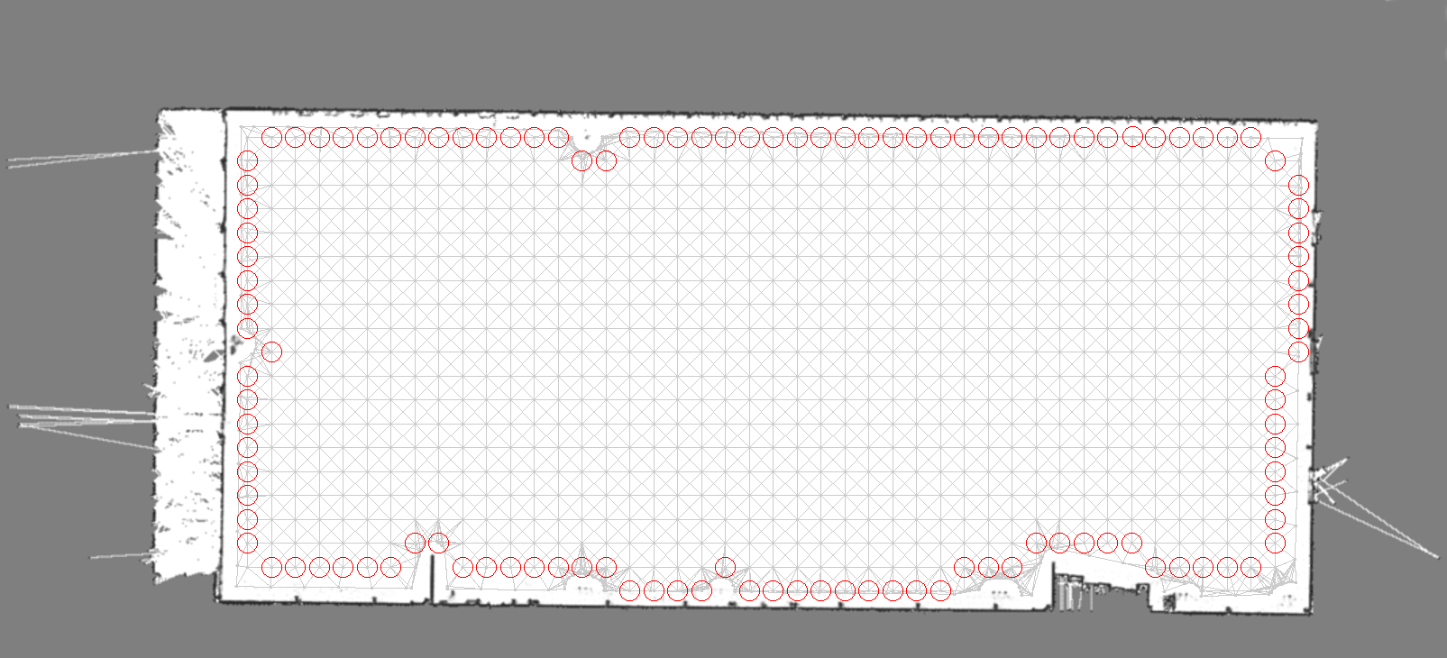
Hall

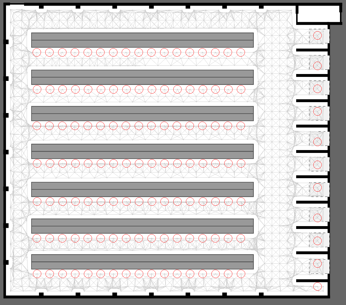
Warehouse

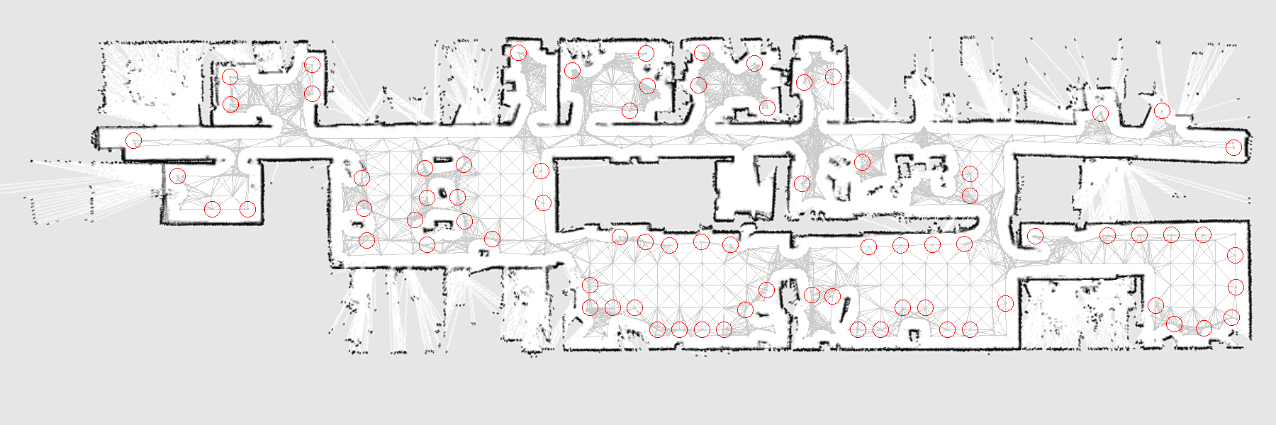
Office

Figure 3: Test environments. The infrastructure endpoints depicted in red, the roadmap graph shown in gray.

Hall	Warehouse	Office

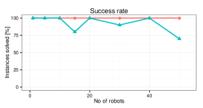
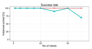
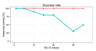
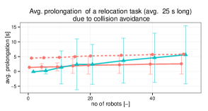
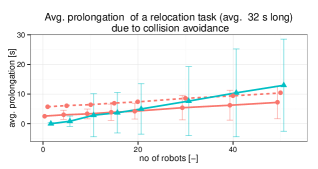
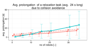
Figure 4: Results. The bars represent standard deviation.

In this section we compare the performance of COBRA and ORCA, a state-of-the art decentralized approach for on-line collision avoidance in large multi-robot teams. The two algorithms are compared in three real-world environments shown in Figure 3. The test environments are valid infrastructures. The execution of a multi-robot system is simulated using a multi-robot simulator. During each simulation, the given number of robots is created and each of them is successively assigned $4$ relocation tasks to a randomly chosen unassigned endpoint. When the simulation is started, all the robots are initialized and the first relocation task with random destination endpoint is issued. To avoid the initial unnatural situation in which all robots would need to plan simultaneously, the initial task is issued with a random delay within the interval [0, 30 s]. Once the robot reaches the destination of its task, a new random destination is generated and the process is repeated until the required number of relocation tasks have been generated. For each such simulation, we observe whether all robots successfully carried out all assigned tasks and the time needed to reach the destination of each relocation task. Further, we compute the prolongation introduced by collision avoidance as $p=t^{A}-t^{\prime}$, where $t^{A}$ is a duration of a particular task when an algorithm $A$ is used for trajectory coordination, and $t^{\prime}$ is the time the robot needs to reach the destination without collision avoidance simply by following the shortest path at the roadmap at maximum speed.

The robots are modeled as circular bodies with radius $r$=50 cm that can travel at maximum speed $v_{\mathrm{max}}$=1 m/s. The relative size of a robot and the environment in which the robots operate is depicted in Figure 3, where the red circles indicate the size of a robot. The roadmaps are constructed as 8-connected grid with additional vertices and edges added near the walls to maintain connectivity in narrow passages. The non-diagonal edges of the base grid are 130 cm long, the diagonal edges are 183 cm long.

The planning window used by COBRA is $t_{\mathrm{planning}}=\text{3\,\ s}$ long, yet on average single planning required only around 0.7 s even on the most challenging instances. The time-extended roadmap uses discretization $\delta t$=650  that conveniently splits travel on the non–diagonal edges into 2 time steps and diagonal edges into 3 time steps.

The reactive technique ORCA (?) is a control-engineering approach typically used in a closed-loop such that at each time instant it selects a collision-avoiding velocity vector from the continuous space of robot’s velocities that is the closest to the robot’s desired velocity. In our implementation, at each time instant the algorithm computes a shortest path from the robots current position to its goal on the same roadmap graph as is used for trajectory planning by COBRA. The desired velocity vector then points at this shortest path at the maximum speed. When using ORCA, we often witnessed dead-lock situations during which the robots either moved at extremely slow velocities or even stopped completely. If any of the robots did not reach its destination in the runtime limit of 10 mins (avg. task duration is less than 33 s), we considered the run as failed.

Results

Figure 4 shows the performance of COBRA and ORCA in the three test environments. The top row of plots shows the success rate of each algorithm on instances with increasing number of robots. In accordance with our theoretical results, we can see that the COBRA algorithm reliably leads all robots to their assigned destinations without collisions. When we tried to realize collision-free operation using ORCA, the algorithm led in some cases the robots into a dead-lock. The problem was exhibited more often in environments with narrow passages as we can see in the success rate plot for the Office environment.

The bottom row of plots shows the average prolongation of a relocation task when either COBRA and ORCA is used for collision avoidance. The total prolongation introduced by COBRA is composed of two components: planning time and travel time. When a new task is used, the robot waits for $t_{\mathrm{planning}}=3\textrm{\,\ s}$ in order to plan a collision-free trajectory to the destination of its new task. Only then, the found trajectory is traveled by the robot until the desired destination is reached. The robots controlled by ORCA start moving immediately because they follow a precomputed policy towards the destination of the current task or a collision-avoiding velocity if a possible collision is detected. Recall that ORCA performs optimization in the continuous space of robot’s instantaneous velocities, whereas COBRA plans a global trajectory on a roadmap graph with a discretized time dimension. In the case of simple conflicts, ORCA can take advantage of its ability to optimize in the continuous space and generates motions where the robots closely pass each other, whereas COBRA has to stick to the underlying discretization, which does not always allow such close evasions. However, when the conflicts become more intricate, the advantages of global planning starts to outweigh the potential loss introduced by space-time discretization. The exact influence of planning in a discretized space-time can be best observed by looking at the data point for instances with 1 robot – these instances do not involve any collision avoidance and thus the prolongation can be attributed purely to the discretization of space-time in which the robot plans. Further, we can observe that the local collision avoidance is less predictable, which is exhibited by the larger standard deviation.

Conclusion

We proposed a novel method for on-line multi-robot trajectory planning called Continuous Best-response Approach (COBRA) and both formally and experimentally analyzed its properties. We have shown that the algorithm has a unique set of features – its time complexity is low polynomial (quadratic in the number of robots) and yet it achieves completeness in a class of environments called valid infrastructures that encompass most human-made environments that have been intuitively designed for efficient transport. Further, our technique is directly applicable to systems with dynamically issued task and can be implemented in a decentralized fashion on heterogeneous robots. We experimentally compared COBRA with a popular reactive technique ORCA in three real-world maps using simulation. The results show that COBRA is more reliable than ORCA and in more challenging scenarios, the planning approach generates trajectories that are up to 48 % faster than ORCA.

References

- [de Wilde, ter Mors, and Witteveen 2013] de Wilde, B.; ter Mors, A. W.; and Witteveen, C. 2013. Push and rotate: cooperative multi-agent path planning. In Proceedings of the 2013 international conference on Autonomous agents and multi-agent systems, 87–94. International Foundation for Autonomous Agents and Multiagent Systems.
- [Erdmann and Lozano-Pérez 1987] Erdmann, M., and Lozano-Pérez, T. 1987. On multiple moving objects. Algorithmica 2:1419–1424.
- [Ghosh 2010] Ghosh, S. 2010. Distributed systems: an algorithmic approach. CRC press.
- [Guy et al. 2009] Guy, S. J.; Chhugani, J.; Kim, C.; Satish, N.; Lin, M.; Manocha, D.; and Dubey, P. 2009. Clearpath: Highly parallel collision avoidance for multi-agent simulation. In Proceedings of the 2009 ACM SIGGRAPH/Eurographics Symposium on Computer Animation, SCA ’09, 177–187. New York, NY, USA: ACM.
- [Hopcroft, Schwartz, and Sharir 1984] Hopcroft, J.; Schwartz, J.; and Sharir, M. 1984. On the complexity of motion planning for multiple independent objects; pspace- hardness of the "warehouseman’s problem". The International Journal of Robotics Research 3(4):76–88.
- [Lalish and Morgansen 2012] Lalish, E., and Morgansen, K. A. 2012. Distributed reactive collision avoidance. Autonomous Robots 32(3):207–226.
- [Spirakis and Yap 1984] Spirakis, P. G., and Yap, C.-K. 1984. Strong np-hardness of moving many discs. Inf. Process. Lett. 19(1):55–59.
- [Standley 2010] Standley, T. S. 2010. Finding optimal solutions to cooperative pathfinding problems. In Fox, M., and Poole, D., eds., AAAI. AAAI Press.
- [Surynek 2009] Surynek, P. 2009. A novel approach to path planning for multiple robots in bi-connected graphs. In Proceedings of the 2009 IEEE international conference on Robotics and Automation, ICRA’09, 928–934. Piscataway, NJ, USA: IEEE Press.
- [Van Den Berg et al. 2011] Van Den Berg, J.; Guy, S.; Lin, M.; and Manocha, D. 2011. Reciprocal n-body collision avoidance. Robotics Research 3–19.
- [Van den Berg, Lin, and Manocha 2008] Van den Berg, J.; Lin, M.; and Manocha, D. 2008. Reciprocal velocity obstacles for real-time multi-agent navigation. In Robotics and Automation, 2008. ICRA 2008. IEEE International Conference on, 1928–1935. IEEE.
- [Čáp et al. 2013] Čáp, M.; Novák, P.; Selecký, M.; Faigl, J.; and Vokřínek, J. 2013. Asynchronous decentralized prioritized planning for coordination in multi-robot system. In Intelligent Robots and Systems (IROS), 2013.
- [Velagapudi, Sycara, and Scerri 2010] Velagapudi, P.; Sycara, K. P.; and Scerri, P. 2010. Decentralized prioritized planning in large multirobot teams. In IROS, 4603–4609. IEEE.
- [Wagner and Choset 2015] Wagner, G., and Choset, H. 2015. Subdimensional expansion for multirobot path planning. Artificial Intelligence 219:1 – 24.