Conformal Frame Dependence of Inflation

Abstract

Physical equivalence between different conformal frames in scalar-tensor theory of gravity is a known fact. However, assuming that matter minimally couples to the metric of a particular frame, which we call the matter Jordan frame, the matter point of view of the universe may vary from frame to frame. Thus, there is a clear distinction between gravitational sector (curvature and scalar field) and matter sector. In this paper, focusing on a simple power-law inflation model in the Einstein frame, two examples are considered; a super-inflationary and a bouncing universe Jordan frames. Then we consider a spectator curvaton minimally coupled to a Jordan frame, and compute its contribution to the curvature perturbation power spectrum. In these specific examples, we find a blue tilt at short scales for the super-inflationary case, and a blue tilt at large scales for the bouncing case.

I Introduction

Scalar fields non-minimally coupled to gravity naturally arise in higher dimensional theories, such us string theory (for examples see Fujii et al. (2003)), and are attractive from a renormalization point of view Lavrov and Shapiro (2010). Such effective field theory can be described within the framework of Scalar-tensor theory of gravity, first introduced by Jordan Jordan (1959) and followed by Brans and Dicke Brans and Dicke (1961), who realised that by means of a field dependent conformal transformation, i.e. a field dependent re-scaling of the metric, the non-minimal coupling can be absorbed and we are left with the usual Einstein-Hilbert action with a scalar field. Thus, this led to the notion of two distinct frames; the Einstein frame where the scalar is minimally coupled, and a Jordan frame where a non-minimal coupling is present. Here and throughout the paper, we define the Jordan frame as the one in which matter fields are minimally coupled with the metric of the frame. Conversely, matter fields have a universal dilatonic coupling with the scalar field in the Einstein frame.

There have been many controversial arguments about the physical equivalence of conformal frames and much effort has been made to clarify the situation Makino and Sasaki (1991); Faraoni and Nadeau (2007); Deruelle and Sasaki (2011); Gong et al. (2011); White et al. (2012); Jarv et al. (2014); Catena et al. (2007); Chiba and Yamaguchi (2013, 2008); Qiu (2012); Li (2014). The general conclusion at the classical level is that although physically equivalent, interpretations differ from frame to frame. On the contrary, it is still unclear whether they are equivalent at the quantum level George et al. (2014) or not Kamenshchik and Steinwachs (2014). To our opinion it seems it needs quantum gravity to settle down this problem at the quantum level.

Inflation is widely accepted as the model of the early universe and is supported by current data Hinshaw et al. (2013); Ade et al. (2014a, b). As scalar fields play an important role in driving inflation, it is of interest to consider the consequences and implications of the case when the inflaton field is non-minimally coupled to gravity. More specifically, we are interested in the case where there is a Jordan frame in which the inflaton field is non-minimally coupled while matter fields are minimally coupled.

However, since there are functional degrees of freedom in the form of the non-minimal coupling, it does not give us any useful insight if we stick to the general case. On the other hand, if we restrict our consideration too strongly, then we would not be able to learn much from it. Here, we focus on a simple but exact model which can be treated analytically, yet allows sufficient varieties in its outcome. Namely, we choose the power-law inflation model Lucchin and Matarrese (1985) which is realised by an exponential potential. We assume this is what we have in the Einstein frame. In this case, the general solution is known analytically Russo (2004); Andrianov et al. (2011).

The purpose of this work is to study how the physics from the matter point of view may vary from frame to frame in the explicit case of power-law inflation. For this purpose a simple way is to start in the Einstein frame and, by means of a conformal transformation, we go to a Jordan frame where matter is defined to be minimally coupled to the metric.

The structure of this work is as follows. In section II we briefly review the general conformal transformation in a scalar-tensor theory, and apply it to power-law inflation. In section III we introduce a curvaton to our model, and study its behaviour in a Jordan frame. It turns out that this simple curvaton model can give rise to an interesting physics from the matter point of view, and therefore may generate interesting features in the CMB angular spectrum. Finally in section IV we summarise the result and discuss its possible imprints in observational data.

II Power-law inflation

The action for a tensor-scalar theory in the Einstein frame reads

$$S_{g}=\int d^{4}x\sqrt{-g}\left(\frac{M_{pl}^{2}}{2}R-\frac{1}{2}g^{\mu\nu}\partial_{\mu}\varphi\partial_{\nu}\varphi-V[\varphi]\right),$$ (1)

where $M_{pl}$ is the Planck mass, $\varphi$ is an inflaton field and the sub-index $S_{g}$ stands for the gravitational sector. After an arbitrary conformal transformation,

$$g_{\mu\nu}=F[\varphi]\tilde{g}_{\mu\nu},$$ (2)

where $F[\varphi]$ is a well-behaved non-zero function, we obtain the corresponding action in a Jordan frame,

$$S_{g}=\int d^{4}x\sqrt{-\tilde{g}}\left(\frac{M_{pl}^{2}}{2}F[\tilde{\varphi}]\tilde{R}-\frac{1}{2}\tilde{g}^{\mu\nu}\partial_{\mu}\tilde{\varphi}\partial_{\nu}\tilde{\varphi}-\tilde{V}[\tilde{\varphi}]\right),$$ (3)

where the scalar field has been redefined by

$$\left(\frac{d\tilde{\varphi}}{d\varphi}\right)^{2}=F[\varphi]\left|1-\frac{3}{2}M_{pl}^{2}\left(\frac{\partial\ln F}{\partial\varphi}\right)^{2}\right|$$ (4)

and the new potential is

$$\tilde{V}[\tilde{\varphi}]=V[\varphi(\tilde{\varphi})]F^{2}[\varphi(\tilde{\varphi})].$$ (5)

According to Gong et al. (2011); White et al. (2012) both actions lead to the same curvature power spectrum and, hence, they are indistinguishable observationally, for example in the Cosmic Microwave Background. Besides, regarding the running of the units Dicke (1962); Faraoni and Nadeau (2007) we assume that after inflation the inflaton settles down to its minimum. As a result, the Einstein and Jordan frames become equivalent.

Thus, one may wonder why should we consider Jordan frames if the Einstein frame is much simpler. In fact, once we take matter into account, one can usually define a frame where matter is minimally coupled to the metric (6) and therefore, as matter is concerned, physical interpretations in that frame are straightforward. In this sense, the gravitational sector, namely the terms composed of the scalar curvature and the inflaton, is generally physically independent of the arbitrary re-scaling function $F[\varphi]$, while the matter sector is not.

To illustrate this, we consider the Jordan frame where a matter field $\chi$ is minimally coupled to the metric,

$$S_{m}=\int d^{4}x\sqrt{-\tilde{g}}{\cal{L}}_{m}[\tilde{g}^{\mu\nu},\chi].$$ (6)

Transforming back to the Einstein frame (2), we are left with a non-minimal coupling of the matter with the inflaton through $F[\varphi]$,

$$S_{m}=\int d^{4}x\sqrt{-g}F^{-2}{\cal{L}}_{m}[F[\varphi]g^{\mu\nu},\chi].$$ (7)

Power-law inflation was first introduced by Lucchin and Matarrese  Lucchin and Matarrese (1985) where it was shown that a scalar field with an exponential potential,

$$V[\varphi]=V_{0}e^{-\lambda\varphi/M_{pl}},$$ (8)

in a flat FLRW background,

$$ds^{2}=-dt^{2}+a^{2}d\textbf{x}^{2},$$ (9)

give rise to an exact power-law solution,

$$a=a_{0}(t/t_{0})^{p}\quad(0<t<\infty)\,,$$ (10)

where $p=2/\lambda^{2}$ and $\lambda^{2}V_{0}t^{2}_{0}=2M^{2}_{pl}(3p-1)$. As a result, this solution describes an initial big bang followed by an eternal expansion. The Hubble and slow-roll parameters are given respectively by

$$H\equiv\dot{a}/a=p/t\,,$$ (11)

$$\epsilon\equiv-\dot{H}/H^{2}=1/p\,,$$ (12)

where a dot refers to the derivative with respect to the proper time $t$. The solution to the scalar field equation,

$$\ddot{\varphi}+3H\dot{\varphi}+V,_{\varphi}=0,$$ (13)

is given by

$$\varphi=\frac{2M_{pl}}{\lambda}\ln(t/t_{0})\,,$$ (14)

Furthermore, comparing (11) and (14) we are led to the equality,

$$\lambda HM_{pl}=\dot{\varphi},$$ (15)

which will be used later.

Following the work of Russo (2004); Andrianov et al. (2011), one can check that $p>1$ corresponds to an inflationary attractor solution, as it can be seen from Fig. 1. Likewise, one can check that there are essentially two types of general solutions corresponding to two distinct initial conditions, i.e. the field starts rolling up or the field starts rolling down the potential. We decided not to consider these solutions further in this work due to not-well-defined initial conditions when computing the curvature perturbation power spectrum. For a detailed review of the solutions, see Russo (2004); Andrianov et al. (2011).

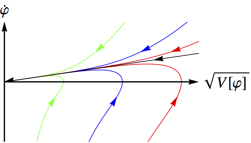
Figure 1: Phase space diagram for a particular $\lambda$. Black line stands for the attractor power-law solution, whereas the colored lines are the two families of general solutions (rolling-up solutions below the black line and rolling-down solutions above the black line).

II.1 Primordial fluctuations

The next stage is to compute the primordial power spectrum for this attractor solution, with the help of cosmological perturbation theory Kodama and Sasaki (1984); Mukhanov et al. (1992). First, we consider the Mukhanov-Sasaki equation for the curvature perturbation Mukhanov (1985); Sasaki (1986),

$$r^{\prime\prime}_{k}+2\frac{z^{\prime}}{z}r^{\prime}_{k}+k^{2}r_{k}=0,$$ (16)

where a prime denotes derivative with respect to the conformal time $d\eta=dt/a$ and

$$z=a\varphi^{\prime}/{\cal H}=\lambda aM_{pl},$$ (17)

where ${\cal H}=a^{\prime}/a$ and we used (15) for the last equality. Second, we assume that the field is in slow-roll regime, i.e. $p\gg 1$, and use the WKB approximation at $k\gg{\cal H}$, yielding the known results Sasaki (1986),

$${\cal P}_{{\cal{R}}_{c}}(k)=\frac{4\pi k^{3}}{(2\pi)^{2}}|r_{k}|^{2}=\left(\frac{H^{2}}{2\pi\dot{\varphi}}\right)^{2}=\frac{p}{8\pi^{2}}\frac{H^{2}}{M^{2}_{pl}}$$ (18)

at $k={\cal H}=Ha$, namely at the horizon crossing time. Rewriting the above in terms of $k$ gives the primordial curvature perturbation spectrum,

$${\cal P}_{{\cal{R}}_{c}}(k)=\frac{p}{8\pi^{2}}\frac{H_{0}^{2}}{M^{2}_{pl}}\left(\frac{k}{k_{0}}\right)^{\frac{-2}{p-1}},$$ (19)

where $k_{0}$ is a reference wavenumber that crosses the horizon at $t=t_{0}$, and $H_{0}=p/t_{0}$. Similarly, the tensor perturbation spectrum is given by

$${\cal P}_{{\cal{T}}}(k)=\frac{4\pi k^{3}}{(2\pi)^{2}}|h_{k}|^{2}=\frac{2}{\pi^{2}}\frac{H^{2}}{M^{2}_{pl}}=\frac{16}{p}{\cal P}_{{\cal{R}}_{c}}(k),$$ (20)

in agreement with the results of standard power-law inflation Lucchin and Matarrese (1985). For a more precise result, see Lyth and Stewart (1992).

Here our main motivation to consider power-law inflation is because the model allows us to study it analytically. Nevertheless, it may be of some interest to check the current status of the observational constraints. The spectral index is given in terms of the parameter $p$ as

$$n_{s}-1=\frac{d\ln{\cal P}_{{\cal{R}}_{c}}}{d\ln k}=\frac{-2}{p-1}\,,$$ (21)

which is slightly red, while the tensor to scalar ratio is given by

$$r=\frac{{\cal P}_{{\cal{T}}}}{{\cal P}_{{\cal{R}}_{c}}}=\frac{16}{p}\,.$$ (22)

The most recent observational constraints are by Planck, which gives $n_{s,planck}\approx 0.96$ and $r_{planck}<0.1$. From the former we obtain $p\approx 50$, but this gives $r\approx 0.32$ which is too large. This is a rather common feature of large field inflation models. However, this discrepancy can be alleviated by invoking a curvaton Moroi and Takahashi (2002); Enqvist and Sloth (2002); Lyth and Wands (2002). Although our purpose is not to resolve the discrepancy but to study the matter’s physics in the Jordan frame, regarding a curvaton as a representative of matter, it turns out that we can actually make power-law inflation observationally more attractive, as will be shown below.

III The matter point of view

In order to understand the matter point of view, we consider an almost massless curvaton $\chi$ Moroi and Takahashi (2002); Enqvist and Sloth (2002); Lyth and Wands (2002) with sub-dominant energy density which plays no role in driving inflation. Therefore the inflationary dynamics is dictated by the inflaton $\varphi$. The action of the spectator curvaton takes the usual form,

$$S_{m}=\int d^{4}x\sqrt{-\tilde{g}}\left(-\frac{1}{2}\tilde{g}^{\mu\nu}\partial_{\mu}\chi\partial_{\nu}\chi-\frac{1}{2}\tilde{m}^{2}\chi^{2}\right)$$ (23)

where $\tilde{g}_{\mu\nu}$ is the metric of a particular Jordan frame and $\tilde{m}$ is the mass of the curvaton in that frame. In general, after a conformal transformation (2) the background is modified,

$$d\tilde{s}^{2}=F^{-1}[\varphi]ds^{2}=-d\tilde{t}^{2}+\tilde{a}^{2}d\textbf{x}^{2},$$ (24)

and the proper time and the scale factor are respectively redefined as

$$d\tilde{t}=F^{-1/2}dt$$ (25)

and

$$\tilde{a}=F^{-1/2}a.$$ (26)

Consequently, the new conformal Hubble parameter is

$$\tilde{\cal H}={\cal H}-F^{\prime}/2F={\cal H}\left(1-\frac{\lambda}{2}\frac{\partial\ln F}{\partial\varphi/M_{pl}}\right),$$ (27)

where (15) has been used.

In passing, for this simple case, it may be worth noting how the frame independence of the quantization is realized inspite of the difference in the physical interpretation. First of all, if the conformal time is used as the time coordinate, the invariance of the canonical commutation relation is trivial. Consequently the invariance of the field equation is also trivial. Nevertheless it is instructive take a look at the differential equation for the mode function in each frame. In the Jordan frame it is

$$\chi^{\prime\prime}_{k}+2\tilde{\cal H}\chi^{\prime}_{k}+(k^{2}+\tilde{m}^{2}\tilde{a}^{2})\chi_{k}=0.$$ (28)

In the Einstein frame where the action is

$$S_{m}=\int d^{4}x\frac{\sqrt{-g}}{F}\left(-\frac{1}{2}g^{\mu\nu}\partial_{\mu}\chi\partial_{\nu}\chi-\frac{1}{2}m^{2}\chi^{2}\right),$$ (29)

where we redefined the mass by $m=F^{-1/2}\tilde{m}$, the equation for the mode functions reads

$$\chi^{\prime\prime}_{k}+2({\cal H}-F^{\prime}/2F)\chi^{\prime}_{k}+(k^{2}+m^{2}a^{2})\chi_{k}=0.$$ (30)

Comparing both (28) and (30), it is clear that they are exactly the same, but their interpretations are rather different. In fact, while (28) is the usual differential equation for the mode functions of a canonical scalar field in a FLRW background, (30) contains explicitly the effect of the non-canonical coupling with the inflaton in the kinetic term.

In any case, the resulting curvaton perturbation spectrum is frame independent. Keeping this in mind, we consider a couple of particular examples below separately. To begin with, we assume a slow-roll inflationary Einstein frame, i.e. $p\gg 1$, unless otherwise noted.

III.1 Power-law Jordan frame

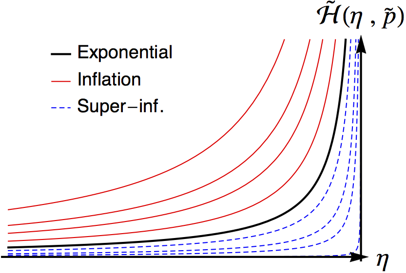
Figure 2: Jordan conformal Hubble parameter as a function of conformal time $\eta$. The black line is the exponential expansion $\tilde{p}\rightarrow\infty$, orange lines stand for power-law inflation, $\tilde{p}>1$, whereas green dashed lines stand for super-power-law inflation, $\tilde{p}<0$.

First we consider a simple conformal transformation,

$$F(\varphi)=\left[V(\varphi)\right]^{-\gamma}=\textrm{e}^{\gamma\lambda\varphi/M_{pl}}=(t/t_{0})^{2\gamma},$$ (31)

inspired by dilaton models in string theory, for example (Blumenhagen et al., 2007). After integrating (4) and substituting it into the Jordan action (3), we are led to

$$S=\int d^{4}x\sqrt{-\tilde{g}}\left(\frac{\xi\tilde{\varphi}^{2}\tilde{R}}{2M^{4}_{pl}}-\frac{1}{2}\tilde{g}^{\mu\nu}\partial_{\mu}\tilde{\varphi}\partial_{\nu}\tilde{\varphi}-V_{0}\Big{(}\frac{\xi\tilde{\varphi}^{2}}{M_{pl}^{2}}\Big{)}^{2-\frac{1}{\gamma}}\right),$$ (32)

where

$$\xi=\frac{(\gamma\lambda)^{2}}{4-6(\gamma\lambda)^{2}}=\frac{\gamma^{2}}{2(p-3\gamma^{2})}\,.$$ (33)

Here we note that for $\gamma^{2}>2/(3\lambda^{2})=p/3$, the gravitational part of the Jordan frame action becomes ghost-like. Nevertheless since the original Einstein frame action is perfectly normal, the system is perfectly stable in spite of its seemingly disastrous appearance Maeda (1989).

In this Jordan frame, we encounter another power-law with a different power law index

$$\tilde{a}=a_{0}(\tilde{t}/\tilde{t}_{0})^{\tilde{p}},$$ (34)

in agreement with Li (2014), where the condition to obtain the scale-invariant tensor spectrum was discussed from the Jordan frame point of view. In (34) we have integrated Jordan time $\tilde{t}$ (25) and replaced into the new scale factor (26), where the Jordan time $\tilde{t}$ now runs from $0$ to $\infty$ for $\tilde{p}>1$ ($\gamma<1$) and from $-\infty$ to $0$ for $\tilde{p}<1$ ($\gamma>1$). Correspondingly, the Jordan power-law index and $\tilde{t}_{0}$ are respectively related to those in the Einstein frame by

$$\tilde{p}-1=\frac{p-1}{1-\gamma}$$ (35)

and

$$\tilde{t}_{0}=\frac{t_{0}}{1-\gamma}.$$ (36)

It is interesting to note that from (35) this Jordan frame is not restricted to $\tilde{p}>1$ nor even $\tilde{p}>0$. Thus, although an almost scale invariant spectrum is obtained independent of the frame, this Jordan frame may not be seen as an inflationary universe from the curvaton point of view, which is subject to the Jordan frame metric. This result reminds us of Tsujikawa (2000), where the non-minimal coupling is used to “assist” inflation. In other words inflation is recovered in the Einstein frame even though the Jordan frame is not inflationary, thanks to the non-minimal coupling of the inflaton.

In this Jordan power-law, we encounter three general cases. First, for $\gamma<1$, we have $\tilde{p}>1$ and the curvaton also feels inflation with a different power-law index. The case $\gamma=1$ corresponds to the exact exponential expansion. Second, for $1<\gamma<p$ we have $\tilde{p}<0$ and the curvaton experiences a super-inflationary universe, where by super-inflationary we mean that the universe expands faster than an exponential expansion. The behavior of the conformal Hubble parameter for $0<\gamma<p$ ($\tilde{p}<0$ and $\tilde{p}>1$) is illustrated in Fig. 2. Finally, for $\gamma>p$, we have $0<\tilde{p}<1$ and the curvaton is in a decelerated contracting universe. Note that $\gamma>p$ implies $\gamma^{2}>p/3$ for $p>1/3$. Hence this last case corresponds to the ghost-like gravity mentioned before.

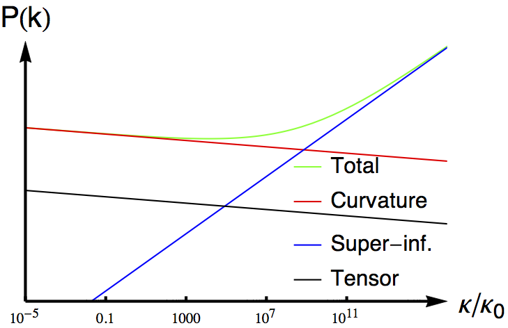
Figure 3: Power spectrum in logarithmic scale for the power-law Jordan case. Inflaton curvature power spectrum (red line), tensor power spectrum (black line), super-inflationary curvaton power spectrum (blue line) and total scalar power spectrum (green line).

In order to compute the scalar power spectrum in this case we assume again that we are in the slow-roll regime, i.e. $|\tilde{p}|\gg 1$, and use the WKB approximation inside the horizon and assume that a mode freezes out instantaneously at horizon crossing, which we call the instantaneous horizon exit assumption. The curvature perturbation spectrum due to the curvaton, under the sudden curvaton decay approximation (Lyth and Wands, 2002), is given by

$${\cal P}_{\chi}(k)=r_{\star}\frac{\delta\chi^{2}}{\chi_{\star}^{2}}=r_{\star}\frac{4\pi k^{3}}{(2\pi)^{2}}\frac{|\chi_{k}|^{2}}{\chi_{\star}^{2}},$$ (37)

where $\chi_{\star}$ is the background value of the curvaton field and $r_{\star}=\rho_{\chi_{\star}}/(\rho+p)_{{\rm tot}_{\star}}$ is the energy density fraction of the curvaton at the time of decay. Note that for (37) to be valid the curvaton must have a non-vanishing background value, which in turn implies $\tilde{H}\gg\tilde{m}$ (Lyth and Wands, 2002; Bartolo and Liddle, 2002). This condition is readily seen from the field equations of motions, i.e.

$$\ddot{\chi}+3\tilde{H}\dot{\chi}+\tilde{m}^{2}\chi^{2}=0,$$ (38)

where requiring $\tilde{H}\gg\tilde{m}$ prevents the curvaton to settle down to its minimum. With the above assumptions we recover the usual scalar power spectrum,

$${\cal P}_{\chi}(k)=r_{\star}\frac{\tilde{H}^{2}}{(2\pi M_{pl}\chi_{\star})^{2}}=r_{\star}\frac{\tilde{H}_{0}^{2}}{M^{2}_{pl}\chi_{\star}^{2}}\left(\frac{k}{k_{0}}\right)^{\frac{-2}{\tilde{p}-1}}\,,$$ (39)

where the total scalar power spectrum is expressed as

$${\cal P}_{\rm tot}={\cal P}_{{\cal{R}}_{c}}+{\cal P}_{\chi}.$$ (40)

As a result, the new tensor to scalar ratio (22) is given by Fujita et al. (2014)

$$\tilde{r}=\frac{r}{1+{\cal P}_{\chi}/{\cal P}_{{\cal{R}}_{c}}}\,.$$ (41)

If we assume the curvaton energy density when it decays to be comparable to or greater than that due to the inflaton, $\tilde{r}$ becomes small enough and the non-gaussianity parameter, $f_{NL}$, becomes $O(1)$ or smaller Enqvist and Takahashi (2013); Byrnes et al. (2014), making this scenario more consistent with the current observational data.

The curvaton spectral index can be easily extracted from (39). We obtain

$$\tilde{n}_{\chi}-1=\frac{-2}{\tilde{p}-1}\,,$$ (42)

which need not be a red index. In particular, a blue tilt can be naturally achieved for $\tilde{p}<0$, that is the super-inflationary situation, which is a common feature of super-inflationary models Piao et al. (2004); Piao and Zhang (2004); Cicoli et al. (2014); Biswas and Mazumdar (2014); Liu et al. (2014); Piao and Zhou (2003). See Fig. 3. This blue spectrum contribution can be important on small scales. For example, it may enhance the primordial black hole formation which can account for a fair amount of dark matter Green (2015). One may fairly wonder how important the back-reaction due to the large curvaton fluctuations would be. This would become important when the amplitude of the power spectrum became of order unity. However, before the back-reaction would become important, one would probably encounter an over-abundance of primordial black holes. This means that there should be a cutoff. Study on such a case may be of interest but it is beyond the scope of the present paper.

III.2 Jordan bouncing universe

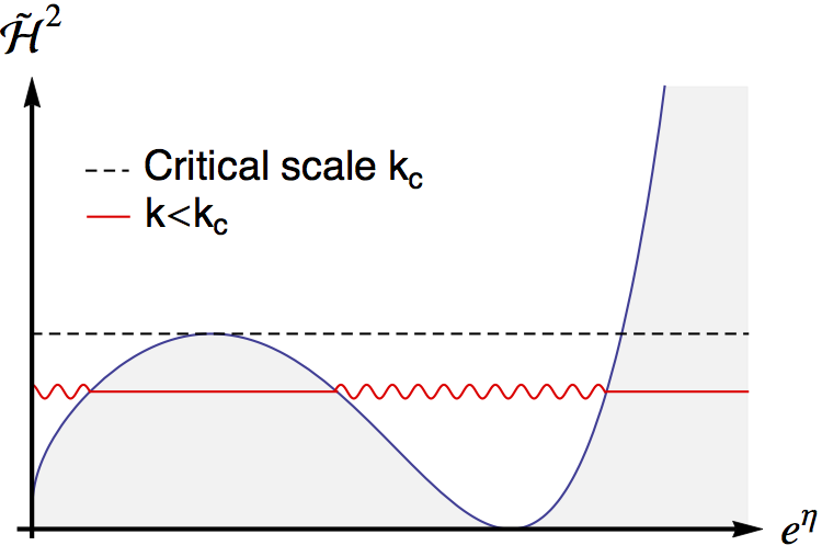
Figure 4: Conformal Jordan squared hubble parameter (blue line) for the bouncing universe case and horizontal lines are constant $k$ lines. Shadowed region stands for super-horizon regime and the consequent freezing of the modes.

As a second example, we consider a conformal transformation of the type,

$$F(\varphi)=\Big{(}1+\textrm{e}^{\frac{-\gamma\lambda}{2M_{pl}}\varphi}\Big{)}^{-2}=\Big{(}1+(t/t_{0})^{-\gamma}\Big{)}^{-2}\,.$$ (43)

For $\gamma>0$ this reproduces the first example, subsection III.1, at early times ($t\ll t_{0}$) and is just identical to the Einstein frame at late times ($t\gg t_{0}$), and it is the other way around for $\gamma<0$. From now on, we focus our attention on the case $\gamma>1$ where the approximate behaviour of the scale factor is

$$\tilde{a}\approx\left\{\begin{array}[]{ccc}a_{0}(-\tilde{t}/\tilde{t}_{0})^{\tilde{p}}&\quad|\tilde{t}|\gg\tilde{t_{0}}&\quad(\tilde{t}<0)\\ a_{0}(\tilde{t}/\tilde{t}_{0})^{p}&\quad\tilde{t}\gg\tilde{t_{0}}\end{array}\right.,$$ (46)

where the Jordan time, $\tilde{t}$ (25), runs from $-\infty$ to $\infty$.

Most interestingly, for the case where $0<\tilde{p}<1$ the curvaton is in a bouncing universe with bounce at

$$t_{bounce}=t_{0}\left(\frac{\gamma}{p}-1\right)^{1/\gamma}.$$ (47)

Note that the big bang singularity in the Einstein frame is sent to $\tilde{t}\to-\infty$ while the bounce occurs at a perfectly regular epoch in the Einstein frame. This model differs from usual bouncing cosmologies Allen and Wands (2004); Lyth (2002); Cai et al. (2007); Qiu et al. (2011) (for a review of bouncing cosmologies see Battefeld and Peter (2015)) in that the initial singularity is avoided from the matter point of view but it is still present in the gravitational sector. In order not to induce any confusion, let us call this a Jordan bouncing universe. In essence, the inflaton is preventing matter to feel the initial singularity through its non-canonical coupling. As a result, in this simple model the curvaton is in a bouncing universe where one can compute the resulting power spectrum due to a well defined initial vacuum state as $\tilde{\cal H}$ vanishes in the limit $\eta\rightarrow-\infty$,

$$\tilde{\cal H}={\cal H}\left(1-\frac{\gamma}{p}\frac{\textrm{e}^{\frac{-\gamma\lambda}{2}\varphi}}{1+\textrm{e}^{\frac{-\gamma\lambda}{2}\varphi}}\right).$$ (48)

Before ending this section, we compute the curvaton power spectrum for the Jordan bouncing universe. It should be noted that, due to the bounce at $\tilde{\cal H}=0$, and a change from a decelerated contracting phase to an accelerated expanding phase at $\tilde{\cal H}^{\prime}=0$, there appears a new critical scale $k_{c}$. See Fig. 4. As schematically shown in the figure, the large scale modes $k<k_{c}$ go out of the Hubble horizon, re-enter the horizon before bounce, and go out of the horizon again during the final inflationary stage, while the small scale modes $k>k_{c}$ remain inside the horizon all through the contractig and bouncing stages until the final inflationary stage.

Moreover, in order for the curvaton to contribute to the scalar power spectrum, it must have a non-vanishing background $\chi=\chi_{0}(\eta)$, which implies that $\tilde{H}\gg\tilde{m}$ has to be satisfied not only at late times but also at early times. We may achieve this condition by assuming an inflaton dependence in the mass of the curvaton, at least $\tilde{m}[\varphi]\propto F^{1/2}[\varphi]$ at early times.

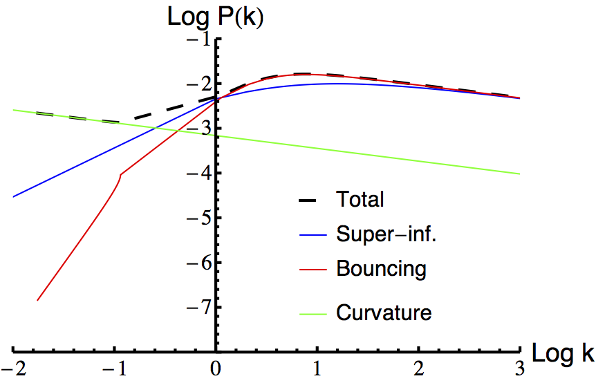
Figure 5: Power spectrum for the bouncing universe (red line), super-inflationary to inflationary universe (blue line), curvature power spectrum (green line) and total scalar power spectrum for the bouncing case (black line).

In this way, with the instantaneous horizon exit and reentry approximation for $k<k_{c}$, the mode functions for the curvaton when they are inside the horizon at the final inflationary stage are given by

$$\chi_{k}\approx\left\{\begin{array}[]{cc}\frac{1}{\sqrt{2k}}\frac{\tilde{a}(\eta_{2})}{\tilde{a}(\eta_{1})}\frac{1}{\tilde{a}(\eta)}\textrm{e}^{-\textrm{i}k\eta+i\alpha_{k}}&\quad k<k_{c}\\ \frac{1}{\sqrt{2k}}\frac{1}{\tilde{a}(\eta)}\textrm{e}^{-\textrm{i}k\eta}&\quad k>k_{c}\end{array}\right.,$$ (51)

where $\eta_{1}$ and $\eta_{2}$ are, respectively, the horizon exit and reentry conformal times for modes with $k<k_{c}$. Although the instantaneous horizon exit and reentry approximation would break down for $\tilde{p}\ll 1$, the resulting power spectrum can be still considered as a rough approximation. Again, making use of (37) we obtain the power spectrum which we compute numerically because of the non trivial form of the scale factor around the bounce. The result is presented in Fig. 5. As may be naively expected, the spectrum becomes blue on large scales.

Lastly, we also consider the case where a super-inflationary phase is present initially $\tilde{p}<0$. In this case we do not need any particular assumption for the mass of the curvaton except for the condition $\tilde{m}\ll\tilde{\cal H}$, and we also obtain a blue spectrum on large scales, as shown in Fig. 5, though the blue tilt is not as sharp as the case of the Jordan bounce.

IV Conclusion

To better understand the role of different conformal frames in cosmology, we considered a simple analytical model in which a scalar field, an inflaton, drives power-law inflation in the Einstein frame, and studied various Jordan frames associated with it by conformally transforming the metric, where a Jordan frame is defined as the frame in which matter is minimally coupled to the metric while the inflaton has a non-minimal coupling with the Ricci scalar. It should be noted that the predictions for both the tensor power spectrum and the curvature perturbation spectrum due to inflaton are unaltered in this setting. They are completely frame-independent and the same as those for the standard power-law inflation.

Particular attention was paid to the physics from the matter point of view. The minimal coupling of matter with a certain Jordan frame metric is equivalent to a dilatonic coupling in the Einstein frame. But this simple difference can lead to a completely different picture of the universe. We studied two examples of how different the universe can be from the matter point of view.

In section III.1 we showed that matter can feel a super-inflationary universe or a decelerating contracting universe, even for a simple conformal transformation, inspired by the dilaton model (31), in spite of having inflation in the gravitational frame, i.e. the Einstein frame. Afterwards, as a representative of matter we considered a curvaton which significantly contributes to the total scalar power spectrum, leaving imprints of its minimal coupling to a particular Jordan metric. For instance, a blue tilt of the power spectrum on small scales can be obtained if the curvaton feels super-inflationary expansion, as shown in Fig. 3, which can enhance the formation of primordial black holes.

In section III.2, we considered another particular conformal transformation (43) which renders matter to feel a bouncing universe and therefore, as far as matter is concerned, the initial singularity is avoided. We obtained again the scalar power spectrum for a spectator curvaton, Fig. 5, which is blue tilted on large scales. In the case where the curvaton mainly generates the total scalar power spectrum, this can give rise to an apparent suppression of the power spectrum at large scales.

To conclude, we emphasise again that the purpose of this paper is not to make specific predictions for a particular class of non-minimal coupling models. With this simple but analytic example what we want to stress is how much the matter point of view, i.e. the Jordan frame point of view, can differ from the gravitational point of view, i.e. the Einstein frame point of view, and how this difference may actually affect observable quantities like the curvature perturbation spectrum.