Magnetohydrodynamic Simulation of the X2.2 Solar Flare
on 2011 February 15: II. Dynamics Connecting the Solar Flare and the Coronal Mass Ejection

Abstract

We clarify a relationship of the dynamics of a solar flare and a growing Coronal Mass Ejection (CME) by investigating the dynamics of magnetic fields during the X2.2-class flare taking place in the solar active region 11158 on 2011 February 15, based on simulation results obtained from Inoue et al. (2014a). We found that the strongly twisted lines formed through the tether-cutting reconnection in the twisted lines of a nonlinear force-free field (NLFFF) can break the force balance within the magnetic field, resulting in their launch from the solar surface. We further discover that a large-scale flux tube is formed during the eruption as a result of the tether-cutting reconnection between the eruptive strongly twisted lines and these ambient weakly twisted lines. Then the newly formed large flux tube exceeds the critical height of the torus instability. The tether-cutting reconnection thus plays an important role in the triggering a CME. Furthermore, we found that the tangential fields at the solar surface illustrate different phases in the formation of the flux tube and its ascending phase over the threshold of the torus instability. We will discuss about these dynamics in detail.

1 Introduction

Solar flares and coronal mass ejections (CMEs) are powerful explosions of the solar coronal plasma that are widely considered to be sudden liberation of the free magnetic energy in the solar atmosphere (Forbes 2000; Priest & Forbes 2002). Our understanding of them is important so that we can not only clarify the nonlinear dynamics of the solar plasma, i.e., the store-and-release processes for magnetic energy and heilicty but also establish the space weather forecast. Since Carrington 1859 discovered the solar flare, many observational, theoretical, and numerical studies have been conducted in order to clarify the properties of solar flares and their relationship with CMEs (Benz 2008; Shibata & Magara 2011).

Carmichael (1964), Sturrock (1966), Hirayama (1974) and Kopp & Pneuman (1976) constructed a flare model based on magnetic reconnection, which well explained observations of solar flares made at multiple wavelengths. This model is named the CSHKP model and is today considered a standard flare model. Since this model was formed, solar physics satellites have provided countless data along with images of the solar flares and CMEs, which are further clarifying their behaviors. In particular, the Yohkoh satellite convinced us of a flare scenario based on the magnetic reconnection (Tsuneta et al. 1992; Masuda et al. 1994). In addition, Yokoyama et al. (2001) discovered clear evidence of reconnection inflows associated with the solar flare from the observations of Yohkoh/SXT and SOHO/EIT. All of these observations built up a foundation of the reconnection model for the solar flare as well as support the classical CSHKP flare model. These observations and theoretical models clarified the properties of solar flares and helped us understand flare physics in a two dimensional regime. On the other hand, our understanding of the dynamics of solar flares is not fully developed in a three dimensional (3D) regime.

Recently, an innovative development of a computer allows us to begin closing this deficiency in our knowledge by performing a 3D magnetohydrodynamic (MHD) simulation to explore solar flare dynamics in 3D space. Antiochos et al. (1999) performed 3D simulation and propose a magnetic breakout model showing an onset of the CME by removing a overly field lines above the core field, through a reconnection. The model has been extended and high resolved simulations are recently performed (e.g., Lynch et al. 2008, Karpen et al. 2012). Amari et al. (2000) and Amari et al. (2003) successfully showed the formation of a flux tube and its eruption via a twist and converging motion on the photosphere from an initial state which starts from a potential field. Török & Kliem (2005) confirmed that the helical kink instability well explains the initial processes of a CME started with anchoring a flux tube in the photosphere and embedding it in the solar corona. They further pointed out that the decrease in the overlying field is a key factor determining whether the resulting eruption fails or is ejective. Forbes (1990) constructed the flux tube model in 2D space and pointed out the eruption via the loss of equilibrium. Following Forbes (1990), Inoue & Kusano (2006) applied a simple straight flux tube in the 3D solar corona; however, Inoue & Kusano (2006) indicated that the flux tube exists in an unstable state against the kink instability before it loses its equilibrium. They further suggested an existence of a critical height deciding whether the eruption is full or failed. Aulanier et al. 2010 and Fan (2010) well-reproduced the initiation of a CME driven by the torus instability (Kliem & Török 2006). Aulanier et al. (2012) brought an interpretation of the CSHKP model into 3D space, explaining the 3D effect, e.g., the strong-to-weak shear transition in the post-flare loop which is not seen in the classical CSHKP model. Kusano et al. 2012 explained that two different types of emerging small fluxes play a role in the triggering mechanisms for the solar flare and CMEs. Recently, a more realistic situation is constructed; where the initial condition mimics a real situation or is applied to a potential field extrapolated from the vector field, enabling us to compare 3D simulations with real observations (e.g., Zuccarello et al. 2012; van Driel-Gesztelyi et al. 2014). More recently, An & Magara (2013), Magara (2013) and Leake et al. (2014) are trying to understand the onset mechanism from their results on the flux emergence simulation without constructing a model.

These 3D simulations show complicated and specific nonlinear dynamics only observable in 3D space. In addition, they interpolate well between 3D dynamics and the observations or models constructed in 2D space. Recently, a solar optical telescope (Tsuneta et al. 2008) and the Helioseismic and Magnetic Imager (Scherrer et al. 2012; Hoeksema et al. 2014) on board the latest solar physics satellite Hinode (Kosugi et al. 2007) and Solar Dynamics observatory (SDO: Pesnell et al. 2012) have provided vector magnetic fields in high temporal and spacial resolutions. These vector fields allow us to reconstruct the 3D coronal magnetic field under a nonlinear force-free field (NLFFF) approximation (Wiegelmann & Sakurai 2012; Régnier 2013) which takes into account even the tangential components of magnetic fields of the vector magnetic fields and is much different from the potential field extrapolated only from the normal component of the vector magnetic fields. The NLFFF exhibits the strong sheared magnetic fields appearing above the polarity inversion line (PIL) prior to the solar flares and CMEs (e.g. Régnier & Amari 2004 or Canou & Amari 2010), as observed by ground and space observations. These are not shown in the potential field. On the other hand, it shows the relaxed magnetic field lines after the flare (Schrijver et al. 2008; Inoue et al. 2012; He et al. 2014). Some papers further clear the temporal evolution of the magnetic field in the active region throughout the flare event (Thalmann & Wiegelmann 2008; Inoue et al. 2011; Sun et al. 2012; Inoue et al. 2013; Jiang et al. 2014; Cheng et al. 2014). However, because these NLFFFs are constructed in the steady sate, they never reveal the dynamics of the solar flares. Therefore, the MHD simulation which takes into account the NLFFF, i.e., data-constrained simulation, are taking a new approach (Jiang et al. 2013; Kliem et al. 2013; Pagano et al. 2013).

More recently, Inoue et al. (2014a) performed the MHD simulation using the NLFFF as an initial condition in order to elucidate the dynamics of the solar flare. This NLFFF is reconstructed 2 hours approximately before the X2.2-class flare in AR11158. The AR11158, which consists of a complicated quadrupole structure, produced several M- and X-class flares in 2011 February (Schrijver et al. 2011; Sun et al. 2012; Inoue et al. 2013) and Hinode and SDO satellites provided rich data observed in multiple wavelengths over the course of the flare events. Inoue et al. (2014a) showed that the dynamics obtained from our MHD simulation successfully reproduced observed phenomena such as the distribution of the two-ribbon flare and the field lines structure as seen in the extreme ultraviolet (EUV) post-flare image taken by Atmospheric Imaging Assembly (AIA; Lemen et al. 2012) which was on board SDO. However, the detailed dynamics of this event are not yet clear.

In this study, we explore the detailed dynamics of the magnetic field during the X2.2 solar flare taking place in AR 11158, based on the simulation results obtained by Inoue et al. (2014a). In particular, we clarify the dynamics connecting the solar flare and the CME, i.e. the geometry and evolution encompassing the region of the flare and CME initiation. This paper is constructed as follows. Our observational data and numerical method are described in Section 2. Our results and discussions are presented in Sections 3 and 4. Our conclusion is summarized in Section 5.

2 NLFFF Extrapolation and MHD Simulation Methods

2.1 Numerical Method and Observations

All of the methods for the NLFFF and MHD simulation following Inoue et al. (2014a). Therefore, here we briefly provide an overview of the numerical methods and observations presented in that work to aid in readers understanding. The NLFFF and MHD simulations are based upon the following equations;

$$\rho=|\mbox{\boldmath$B$}|,$$ (1)

$$\frac{\partial\mbox{\boldmath$v$}}{\partial t}=-(\mbox{\boldmath$v$}\cdot\mbox{\boldmath$\nabla$})\mbox{\boldmath$v$}+\frac{1}{\rho}\mbox{\boldmath$J$}\times\mbox{\boldmath$B$}+\nu\mbox{\boldmath$\nabla$}^{2}\mbox{\boldmath$v$},$$ (2)

$$\frac{\partial\mbox{\boldmath$B$}}{\partial t}=\mbox{\boldmath$\nabla$}\times(\mbox{\boldmath$v$}\times\mbox{\boldmath$B$}-\eta_{i}\mbox{\boldmath$J$})-\mbox{\boldmath$\nabla$}\phi,$$ (3)

$$\mbox{\boldmath$J$}=\mbox{\boldmath$\nabla$}\times\mbox{\boldmath$B$},$$ (4)

$$\frac{\partial\phi}{\partial t}+c^{2}_{h}\mbox{\boldmath$\nabla$}\cdot\mbox{\boldmath$B$}=-\frac{c^{2}_{h}}{c^{2}_{p}}\phi,$$ (5)

where the subscript $i$ of $\eta$ corresponds to ’NLFFF’ or ’MHD’. The length, magnetic field, density, velocity, time, and electric current density are normalized by $L^{*}$ = 216 Mm, $B^{*}$ = 2500 G, $\rho^{*}$ = $|B^{*}|$, $V_{A}^{*}\equiv B^{*}/(\mu_{0}\rho^{*})^{1/2}$, where $\mu_{0}$ is the magnetic permeability, $\tau_{A}^{*}\equiv L^{*}/V_{A}^{*}$, and $J^{*}=B^{*}/\mu_{0}L^{*}$, respectively. The non-dimensional viscosity $\nu$ is set as a constant $(1.0\times 10^{-3})$, and the coefficients $c_{h}^{2}$, $c_{p}^{2}$ in equation (5) also fix the constant values, 0.04 and 0.1, respectively. Although the density is given as a model like Amari et al. (1996), we previously discussed its validity in Inoue et al. (2014a).

The vector magnetic field that we used as the boundary condition is observed at 00:00 UT on February 15, approximately 2 hours before the X2.2-class flare was detected by HMI/SDO. It covers a 216 $\times$ 216 (Mm²) region, divided into a 600 $\times$ 600 grid. It is obtained using the very fast inversion of the Stokes vector (VFISV) algorithm (Borrero et al. 2011) based on the Milne$-$Eddington approximation. A minimum energy method (Metcalf 1994; Leka et al. 2009) was used to resolve the 180^∘ ambiguity in the azimuth angle of the magnetic field. In this study, the vector field is preprocessed in accordance with Wiegelmann et al. (2006).

A numerical box with dimensions of 216 $\times$ 216 $\times$ 216 (Mm³) is given by 1 $\times$ 1 $\times$ 1 as a non-dimensional value. 2 $\times$ 2 binning of the original data yields grid numbers which are assigned as 300 $\times$ 300 $\times$ 300. The detailed numerical scheme is available in Inoue et al. (2013) or Inoue et al. (2014b).

2.2 NLFFF Extrapolation

We first perform an NLFFF extrapolation to obtain the 3D structure of the magnetic field prior to the X2.2-class flare, and to understand its physical properties relating to stability; we apply the MHD simulation as an initial condition. This is based on the MHD relaxation method developed by Inoue et al. (2014b) which shows the detailed algorithm. The initial condition is given by a potential field obtained from the Green function method (Sakurai 1982). At the boundaries, the three components of the magnetic field are fixed; in particular, the three observed components of the magnetic fields are set at the bottom boundary and their velocities are set as zero. The Neumann boundary condition is imposed on $\phi$. A formulation of $\eta$ is given by

$$\eta_{nlfff}=5\eta_{0}+\eta_{1}\frac{|\mbox{\boldmath$J$}\times\mbox{\boldmath$B$}||\mbox{\boldmath$v$}|^{2}}{\mbox{\boldmath$|B|^{2}$}},$$ (6)

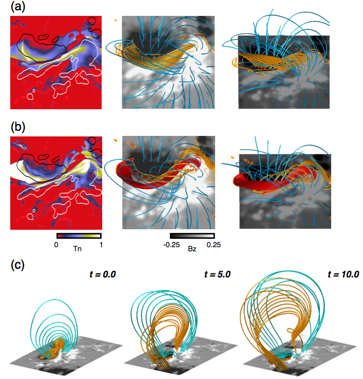
Figure 1: (a) The left panel is a distribution of the magnetic twist of the NLFFF 2 hours approximately before the X2.2-class flare, with contours of $B_{z}$ where black and white contours correspond to $B_{z}$=0.25(625 G), and -0.25, respectively. The field lines begin in the region (0.35$L_{0}$ $<$x$<$ 0.65$L_{0}$ and 0.4$L_{0}$ $<$y$<$ 0.7$L_{0}$, where $L_{0}$ is 216 Mm ). Then the magnetic twist is mapped, where the value of $|B_{z}|$ is more than 0.01 (=25 G). The middle panel shows the field line structure. The orange curves show twisted lines with more than a half-turn twist while the blue lines have less than a half-turn twist. The Right panel also represents the 3D structure of the field lines from another angle. (b) The twist distribution and 3D field line structure after the MHD relaxation process. The figure format is the same as (a), except the red lines show the strongly twisted lines with more than a one-turn twist. (c) The temporal evolution of the magnetic field obtained from the MHD simulation. The orange and blue lines have twisted lines more and less than a half-turn twist, respectively, at an initial time $t$=0.0.

where $\eta_{0}$=$1.0\times 10^{-5}$ and $\eta_{1}$=$1.0\times 10^{-3}$. The NLFFF is performed in the center area of AR11158 to avoid any effects from the inconsistent force-free $\alpha$, and outside it is fixed by the potential field (see Figure 1(a) in Inoue et al. 2014a). This calculation corresponds to Run A in Table 1 as shown in Inoue et al. (2014a). Figure 1(a) shows a distribution of the magnetic twist and 3D field lines structure in the central area of AR11158. Magnetic twist is defined by

$$T_{n}=\frac{1}{4\pi}\int\frac{J_{||}}{|\mbox{\boldmath$B$}|}dl,$$ (7)

where $J_{||}=\mbox{\boldmath$J$}\cdot\mbox{\boldmath$B$}/|\mbox{\boldmath$B$}|$ and $dl$ is a line element (Berger & Prior 2006). We found that the strong magnetic twist of the NLFFF is distributed in the range from a half-turn to one-turn twist. Inoue et al. (2014a) found that the NLFFF exists in a stable state not only against an ideal MHD instability, such as a kink or torus instability, but also against even a small perturbation. In other words, this NLFFF needs to be excited into a higher energy level to release the free magnetic energy required to produce the flare.

2.3 MHD Relaxation and Simulation

We further perform the MHD relaxation using the NLFFF as an initial condition to excite it into higher energy level. We employ the zero-$\beta$ MHD equations which are the same as those used in the NLFFF calculation, except the velocity limiter is released (see Inoue et al. 2014b) and the resistivity formulation is replaced by the anomalous one as follows,

$$\eta_{MHD}(t)=\left\{\begin{array}[]{ll}\eta_{0}&\quad\mbox{$J<j_{c}$},\\ \eta_{0}+\eta_{2}(\frac{J-j_{c}}{j_{c}})^{2}&\quad\mbox{$J>j_{c}$},\end{array}\right.$$ (8)

where $\eta_{2}=5.0\times 10^{-4}$, and $j_{c}$ is the threshold current, set to 30 in this study. The boundary condition is same as a case of the NLFFF. Because the anomalous resistivity can enhance a reconnection in the strong current region between the twisted lines formed in the NLFFF, we can expect it to form stronger twisted lines. This calculation corresponds to Run C in Table 1 as shown in Inoue et al. (2014a). Figures 1(b) shows the distribution of the magnetic twist and 3D field lines structure after the MHD relaxation process, these are same format with Figure 1(a). We found that the strongly twisted lines with more than a one-turn twist are formed after the MHD relaxation process, which are not shown in the original NLFFF, as shown in Figure 1(a). The formation of these strongly twisted lines is clearly due to the anomalous resistivity, which is reminiscent of the tether-cutting reconnection.

Finally, we perform the MHD simulation using the magnetic field shown in Figure 1(b) obtained after the MHD relaxation process. At the boundaries, the tangential components of the magnetic field are released to interact with an induction equation consistently, while the normal component of the field remains constant. Note that in this case, the tangential components gradually go back toward the state of the potential field (or another less twisted state) because the NLFFF cannot maintain the force-free state completely. The velocity and $\phi$ are treated in the same manner for all boundaries as were the NLFFF calculation and time-relaxed simulation. This calculation corresponds to Run D in Table 1 as shown in Inoue et al. (2014a). The magnetic field shown in Figure 1(b) is already in a non-equilibrium state;therefore, it illustrates the dramatic dynamics shown in Figure 1(c). An overview of these is was summarized in Inoue et al. (2014a).

3 Results

Inoue et al. (2014a) presented the overview of the dynamics and compared these with some observations. In this paper, we study the more detailed 3D dynamics, in particular, focusing on the formation of the large flux tube, i.e., the growing process of the CME, and other phenomena associated with the reconnection, eventually understanding a relationship flares and CMEs.

3.1 Temporal Evolution of the Magnetic Twist

In general, 3D dynamics obtained from the MHD simulation show a complicated behavior, so it is not easy to extract essential components from them. However, the magnetic twist defined in equation (7) is one solid tool that we can use to extract these components, e.g., a dynamics of flux tube and the reconnection associated with the formation and dynamics of the flux tube. Because the flux tube consists of a bundle of field lines with a strong magnetic twist, we can trace the temporal evolution of the flux tube by tracing that of the magnetic twist. Furthermore, since the magnetic twist is a magnetic helicity generated by a toroidal current in the flux tube (Berger & Prior 2006; Török et al. 2010; Inoue et al. 2012 ), the magnetic twist would help us understand the reconnection dynamics in terms of conservation law of the magnetic helicity.

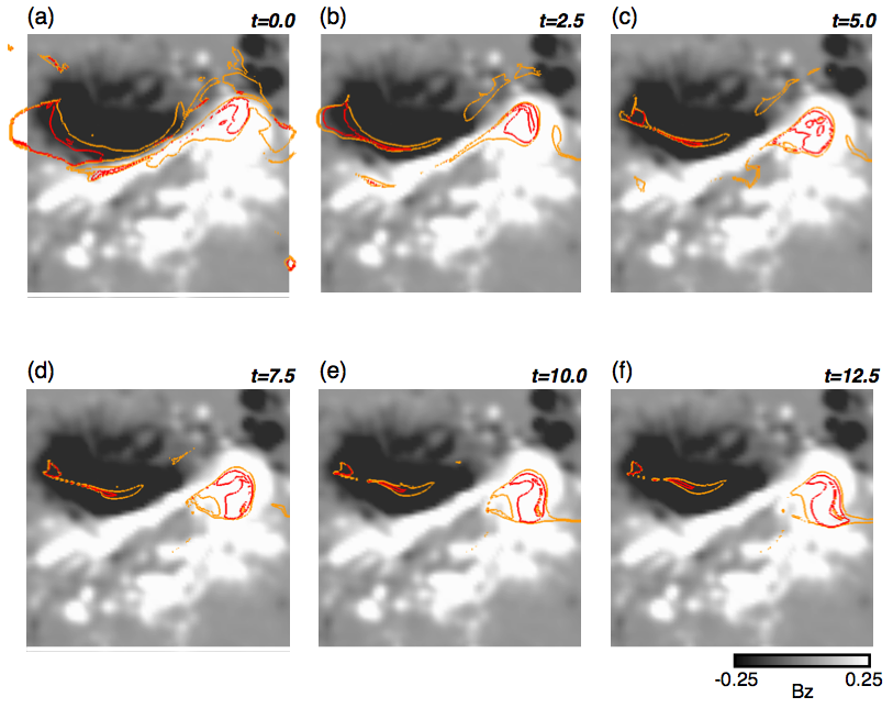
Figure 2: Temporal evolution of the magnetic twist mapped on the solar surface, focusing on the central region of AR11158. The $B_{z}$ distribution is represented in gray scale. The red and orange lines are contours of the magnetic twist $T_{n}=1.0$ and $T_{n}=0.5$, respectively. Note that the inside regions surrounded by the red and orange lines are occupied by the strongly twisted lines.

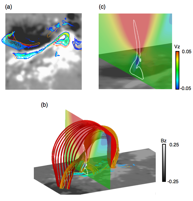
Figure 8: (a) $\Delta(\mbox{\boldmath$x$}_{0},4.0)$ is mapped on the $B_{z}$ distribution at the solar surface with the twist contours, $T_{n}=$0.5 and $T_{n}$=1.0 in orange and red, respectively. (b) The field lines structure at $t=$4.0. The figure format is the same as that in Figure 6(c), except the contour of the current density $|\mbox{\boldmath$J$}|$=5.0 is plotted in white, and the vertical velocity distribution is plotted on the vertical cross section. (c) The vertical velocity close to the strong current region is plotted with the current density contour $|J|$=5.0.

We first show in Figure 2 the temporal evolution of the magnetic twist during the flare obtained from the MHD simulation, mapped on the solar surface where $T_{n}=1.0$ and $T_{n}$=0.5 are plotted. The locations surrounded by the contour of $T_{n}$=1.0 and 0.5 correspond to where the base of the flux tube exists. We clearly see that the locations of the twisted flux tube are not fixed;rather, they move in a course. At positive polarity, the region occupied by the strong magnetic twist is moving southward. The region located at the negative polarity is shrinking in an early phase and then seems to maintain its size in a later phase. These are not simple pictures that we can image easily, particularly since they are occurring in 3D space. Furthermore, although the twist is widely distributed in the area close to the polarity inversion line (PIL) at initial time, it seems to be concentrated in the area away from the PIL at $t$=12.5. In other words, most of the strongly twisted lines disappear close to the PIL. The reason for this is that the post-flare loops are formed through reconnection during the flare, as shown in Figure 8(a) of Inoue et al. (2014a).

3.2 Formation of the Large Flux Tube

We see the temporal evolution of the magnetic field lines in Figure 3, where we focus on the strongly twisted lines in red which have more than one-turn twist and those in blue which have less than a one-turn twist (since most parts are less than half-turn, hereafter we call them weakly twisted lines). These weakly twisted lines are traced from the location close to where the strongly twisted lines exit. Although the strongly twisted lines with more than a one-turn twist launch away from the solar surface, they split into two parts in an early phase, $t$=2.5; one footpoint of some field lines is rooted in the negative polarity at southeast area which locates away from the central area. That is why we see that the strongly twisted region occupied on central negative polarity shrinks (see Figure 2). Interestingly, the weakly twisted lines enter the large flux tube, while the short twisted lines marked by the arrow in Figure 3 are left where the strongly twisted lines existed at $t$=0.0. The contour of the strong twists ($T_{n}$=1.0) is plotted on the solar surface at $t$=0.0 and $t$=12.5. At $t$=0.0 the footpoint of the red field lines is rooted in the region surrounded by the contour of $T_{n}$=1.0, while at $t$=12.5 this contour surrounds the footpoint of the blue field lines.

This result indicates that the twisted lines that were initially weak convert into the large flux tube having strongly twisted lines with more than a one-turn twist. This process might be explained by the tether-cutting reconnection between the eruptive strongly twisted lines in red and ambient weakly twisted lines in blue, because the weakly twisted lines can receive magnetic helicity from the strongly twisted lines via reconnection processes. Therefore, the strongly twisted region on the central positive polarity moves the southern region occupied by the weakly twisted lines as seen in Figure 2.

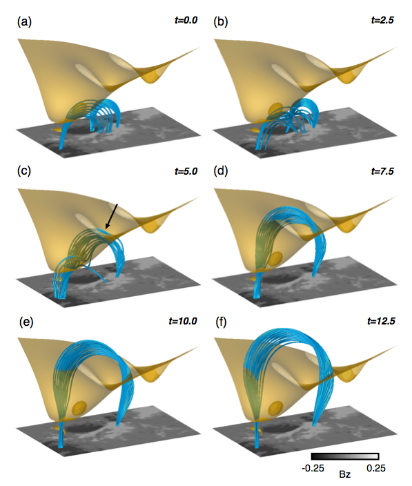
Figure 4: Temporal evolution of the dynamics of the magnetic field lines from side view of Figure 3. The field lines format is same in Figure 3, except the temporal evolution of the initial strongly twisted lines with more than a one-turn twist is not plotted. The yellow surface corresponds to a critical height of the torus instability, i.e, the isosurface with decay index $n$=1.5 where $n$ is defined by equation (9). Arrow points towards the intersection of the magnetic field lines and the threshold of the instability.

Figure 4 also shows the temporal evolution of the magnetic field lines from another angle, plotted in the same format as Figure 3, except that the evolution of the strongly twisted lines is omitted. The yellow surface corresponds to the critical height of the torus instability, i.e., a decay index of $n$=1.5 where $n$ is defined by

$$n(z)=-\frac{z}{|\mbox{\boldmath$B$}|}\frac{\partial|\mbox{\boldmath$B$}|}{\partial z},$$ (9)

where, the decay index is calculated based on the potential field. Because the decay index is derived from the external poloidal field sustaining the hoop force by the flux tube(Török & Kliem 2007), it is difficult to separate the external field from the NLFFF, following Fan & Gibson (2007) and Aulanier et al. (2010). This result clearly shows that the weakly twisted lines reform into large and strongly twisted lines through reconnection before reaching the critical height of the torus instability. After this, the top of the field lines exceed the critical height and would further grow into the CME.

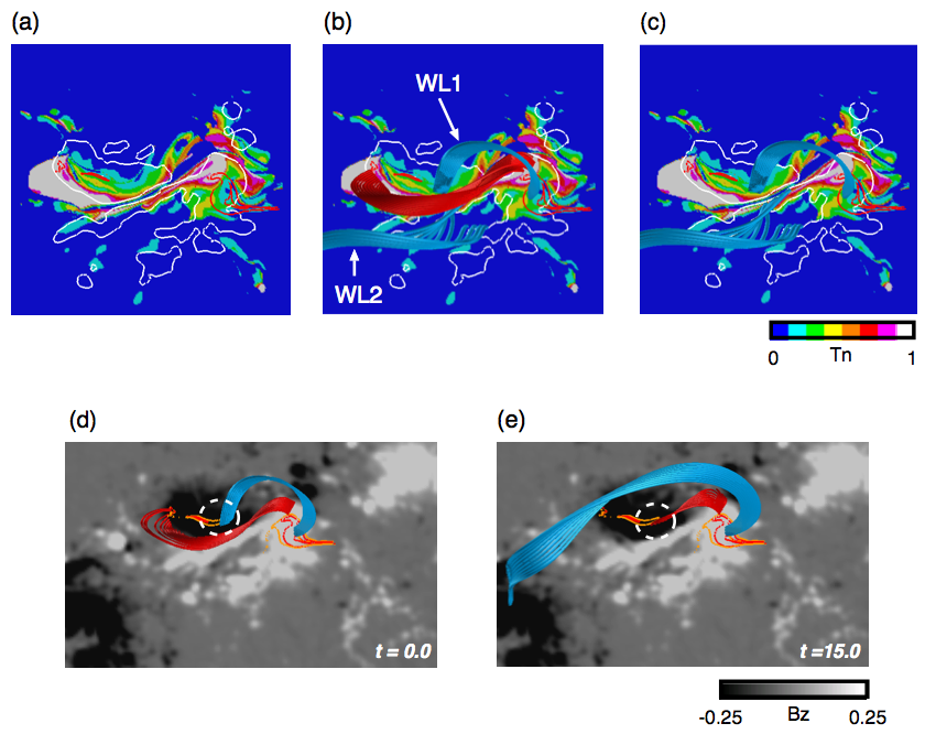
Figure 5: (a) The distribution of the twist at $t$=0.0 with contours of $T_{n}$=1.0 at $t$=15.0 in red and $|B_{z}|$=0.25 in white. (b) The field lines at $t$=0 are plotted over (a). The format of these field lines are same as Figure 3. (c) The same field lines at $t$=0.0 are plotted over (a) except the strongly twisted lines in red are not plotted. (d) The twisted lines at $t$=0.0 are plotted in red and blue, traced from the positive polarity. The contours of twist $T_{n}$=0.5, and 1.0 at $t$=15.0 are plotted in red and orange, respectively, over the $B_{z}$ distribution where the twisted lines in blue are started from the inside region surrounded by the contour $T_{n}$=1.0 at $t$=15.0. (e) The same format with (d) except the field lines are plotted at $t$=15.0.

We carry out a more detailed quantitative analysis in terms of the conservation of magnetic helicity. Figure 5(a) displays the distribution of the magnetic twist at $t$=0.0 with the contours of $T_{n}$=1.0 at $t$=15.0 and $B_{z}$. Although one footpoint of the large flux tube formed during the flare is observed within a region surrounded by the red line in Figure 5(a), the twist value of the field lines at this location at $t$=0.0 is less than 0.375 turns, approximately. The twisted field lines at $t$=0.0 are plotted in Figure 5(b), where the red twisted lines have more than a one-turn twist while one of the blue twisted lines, ’WL1’, has less than 0.375 turn twist approximately and another blue twisted line, ’WL2’ has a twist close to zero. However, very few field lines in ’WL2’ have more than a half-turn twist, as shown in Figure 5(c). If the tether-cutting reconnection takes place only between the field lines ’WL1’ and ’WL2’ , then the long twisted lines with more than a one-turn twist are never produced, since by the conservation law of the magnetic helicity. WL1 and WL2 do not supply the twist enough to form such lines. This large flux tube is, therefore, formed through the reconnection between the weakly twisted lines ’WL1’, and ’WL2’, and strongly twisted lines which are a source supplying the magnetic helicity.

The field lines at $t$=0.0 and $t$=15.0 traced from the same location on the positive polarity are plotted with $B_{z}$ distribution and contours of $T_{n}$=0.5 and 1.0 at $t$=15.0 in Figures 5(d) and (e), respectively. As we presented in Figure 3, at $t$=15.0 the blue twisted lines become strongly twisted lines, even though they were weakly twisted at $t$=0.0. Eventually, the footpoint of the red field lines dominates at $t$=15.0 at a location marked by the dashed white circle, which is where the blue field lines resided at $t$=0.0. These results also support that magnetic reconnection takes place between the strongly twisted lines and weakly twisted lines, WL1 and WL2;consequently, part of the red lines remain at the solar surface at $t$=15.0 as sheared post-flare loops. Thus, some of the magnetic helicity accumulated into the strongly twisted lines at $t$=0.0 is transferred into the weakly twisted lines through the reconnection, resulting in the formation of the large strongly twisted lines.

3.3 Reconnection Dynamics in the X2.2 Solar Flare

We investigate the reconnection process in the early flare phase. Following Toriumi et al. (2013) and Inoue et al. (2014a), we estimate the reconnected field lines by using a spatial variance of the field line connectivity by allowing them only by reconnection. The formulation is defined by the following equation:

$$\delta(\mbox{\boldmath$x$}_{0},t_{n})=|\mbox{\boldmath$x$}_{1}(\mbox{\boldmath$x$}_{0},t_{n+1})-\mbox{\boldmath$x$}_{1}(\mbox{\boldmath$x$}_{0},t_{n})|\quad(\mbox{$T_{n}\geqq 0.3$}),$$

where $\mbox{\boldmath$x$}_{1}(\mbox{\boldmath$x$}_{0},t_{n})$ is the location of one footpoint of each field line at time ${\it t_{n}}$, which is traced from another footpoint at $\mbox{\boldmath$x$}_{0}$. Eventually, we calculate

$$\Delta(\mbox{\boldmath$x$}_{0},t)=\int_{0}^{t}\delta(\mbox{\boldmath$x$}_{0},t_{n})dt_{n},$$ (10)

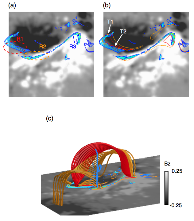
Figure 6: (a) $\Delta(\mbox{\boldmath$x$}_{0},2.0)$ is mapped on the $B_{z}$ distribution where $\Delta(\mbox{\boldmath$x$}_{0},2.0)$ is measured at $|B_{z}|>0.01$ and $T_{n}\geqq$0.3. (b) The contours of the twist $T_{n}$ = 0.5 and 1.0 are plotted in the orange and red lines with $\Delta$ map over the $B_{z}$ distribution. (c) The 3D magnetic field line structure is plotted over (b). The red lines represent the strongly twisted lines with more than a one-turn twist, while the orange field lines are passing through the region surrounded by the blue line, which is a contour of the current density ($|J|$=5.0).

where the enhanced region in $\Delta(\mbox{\boldmath$x$}_{0},t)$ indicates memories in which the reconnection took place dramatically in the twisted lines. Figure 6(a) shows the distribution of $\Delta(\mbox{\boldmath$x_{0}$},t=2.0)$ over the $B_{z}$($>$0.01) distribution, which we previously discussed, and this shape is similar to that of an observed two-ribbon flare (Inoue et al. 2014a.) Figure 6(b) shows the $\Delta$ map with the twist contours $T_{n}$=0.5 and 1.0 over the Figure 6(a). From this figure we found that the enhanced region ’T2’ is found just outside of the region containing the strongly twisted lines, while the region ’T1’ overlaps with their insides. We can find the same profiles on the positive polarities. Figure 6(c) shows the 3D magnetic field lines, where the red field lines indicate the strongly twisted lines with more than a one-turn twist and where the orange lines go through an inner part of the region surrounded by the current density $|\mbox{\boldmath$J$}|$=5.0 contour. In an earlier flare phase the strongly twisted lines with more than a one-turn twist erupt away from the solar surface, beneath which the orange field lines are reconnected, forming the long twisted lines and post-flare loops on the $\Delta$ map.

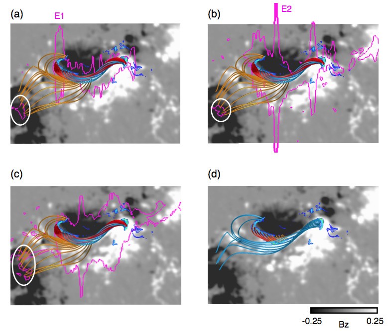
Figure 7: (a)-(c) The field lines at $t$=0 are plotted with the contour of AIA intensity and $\Delta(\mbox{\boldmath$x$}_{0},2.0)$ over the $B_{z}$ distribution. Each colored field line is traced from each colored region, R1, R2, and R3 marked in Figure 6(a). The purple lines correspond to the AIA intensity $log(I)$=9.0 at 01:50:25 UT, 01:52:49 UT and 02:04:49 UT from (a) to (c) where the first two correspond to the much earlier flare phase and the latter is in the middle flare phase. (d) Each colored field line at $t$=2.0 is plotted over (a), but AIA intensity is not plotted.

We investigate the relationship between the field lines structure and EUV images taken by SDO to further understand the reconnection dynamics. Figures 7(a)-(c) represent the field lines structure at $t$=0, where each colored field line( red, orange, and blue) is traced from the regions, R1, R2, and R3 surrounded by dashed circles in Figure 6(a). The intensity contour taken from an AIA 171 Å image is also plotted with these field line structures, where Figures 7(a) and (b) show the much earlier flare phase and Figure 7(d) exhibits it in middle flare phase. In Figures 7(a) and (b), the most enhanced areas are located at E1 and E2 for each time where the small flux tubes are coexisting, e.g., we can see the red and orange field lines at E1 and three different field lines at E2. This means that the reconnection might take place among these small flux tubes. Figure 7(d) shows the field lines structure $t$=2.0. The field lines traced from the regions R1 and R2 convert into post-flare loops, on the other hand, some of footpoint in blue traced from R3 are rooted into the hook region on another polarity in which the contours of the strongly twisted lines are also observed, as shown in Figure 6(b). Another footpoint is rooted into the negative polarity located southeast away from the central area. This location is marked by a solid white circle at each time in Figures 7(a)-(c), in which EUV images are enhanced during the flare. These results demonstrate that the location close to the PIL is crowded with some twisted lines, i.e., small flux tubes, before the flare, and then the complicated reconnection takes place among them during the flare.

We also checked the $\Delta$ map and 3D magnetic field at $t$=4.0. Figure 8(a) shows the $\Delta(\mbox{\boldmath$x$}_{0},t=4.0)$ with the twist contours mapped on the bottom surface in the same format as that in Figure 6(b), and it well resembles the two-ribbon flare structure (see Inoue et al. 2014a). Figure 8(b) exhibits the 3D structure of field lines in the same format as Figure 6(c), except the distribution of the vertical velocity is plotted on the vertical cross section. Figure 8(c) shows the enlarged view of the current layer and the distribution of vertical velocity close to the solar surface. We clearly see the upward and downward flows, which have an origin at the inner side of the current layer, meaning that the reconnection is occurring here. The strongly twisted lines in red are a slightly different from that seen in Figure 6(c). We can see that one footpoint is rooted into the negative polarity located southeast away from the central region. This result indicates that the strongly twisted lines also interact with the ambient twisted lines during their ascension, as suggested by Figure 3. The orange field lines show similar behavior as that seen in Figure 6(c). Through reconnection, the field lines convert into the long twisted field line, whose one footpoint is rooted into the negative polarity in the southeast, and the post-flare loops. Figure 8(b) also clearly shows that the locations of both footpoints of the post-flare loops correspond to those in which the $\Delta$ maps exist.

3.4 Comparisons with the Observations

3.4.1 Enhancement of the Tangential Field at Solar Surface

In this section, we compare our simulation results with some observations to evaluate the validity of our reconnection dynamics.

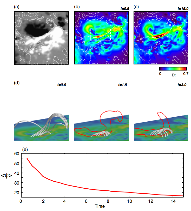
Figure 9: (a) $B_{z}$ distribution with a polarity inversion line in white is plotted in the range of 0.33$<$x$<$0.63 and 0.37$<$y$<$0.67. (b)-(c) The distribution of the tangential components of the magnetic field $B_{t}$=$\sqrt{B_{x}^{2}+B_{y}^{2}}$ at $t$=0.5 and $t$=15.0. (d) The structure of field lines in the early flare phase is plotted in gray. The field lines shown in (e) and (f) are plotted passing through the inside of the current contour $|\mbox{\boldmath$J$}|$=10. The field lines in (d) are traced from same points in (e). The bottom surface represents the distribution of $B_{t}$, which is in the same format as (b) and (c). (e) A temporal evolution of an averaged shear angle between the tangential fields in the simulation and that of the potential fields, measured on $B_{t}>$ 0.4 at the solar surface, surrounded by white dashed square(0.433$<$x$<$0.533 and 0.50$<$y$<$0.567). depicted in (a). The unit is degree.

Wang et al. (2012) discovered an enhancement of the tangential magnetic fields during the flare, residing in a location close to the PIL on the solar surface. They, as well as Sun et al. (2012), suggested that this enhancement is strongly related to the reconnection. We check this with the temporal evolution of the tangential fields ($B_{t}$=$\sqrt{B_{x}^{2}+B_{y}^{2}}$) obtained from our simulation. Figure 9(a) shows the $B_{z}$ distribution in the central area in which the tangential fields are measured. Figures 9(b) and (c) represent the distribution of the tangential magnetic fields at $t$=0.5, and $t$=15.0, respectively. We clearly see that the tangential fields are strongly enhanced at a location close to the PIL, whose value can reach more than 2000 G. These values and locations are therefore well consistent with those observed by Wang et al. (2012).

The structure of field lines is depicted in an early flare phase above the enhancement of $B_{t}$ at the photosphere, at $t$=0.0, 1.5, and 3.0 in Figures 9(d), respectively. At $t$=0.0, just after the MHD relaxation process, the long sheared field lines are formed, and then they convert into the short loops at $t$=1.5. Since these short field lines pass through the strong current region, we can interpret that these correspond to post-flare loops formed through the reconnection. Furthermore, $B_{t}$ is enhanced under the area in which the post-flare loops reside, even in the early phase at $t$=1.5. At $t$=3.0, we found that $B_{t}$ is more enhanced and the taller post-flare loops are formed, above which the further new post-flare loops are being produced and piled up through sequential reconnection. This result implies that the tangential field of the newly formed post-flare loops sufficiently compresses the pre-existing ones below, resulting in the enhancement of the tangential magnetic fields near the solar surface.

In Figure 9(e), we show a temporal evolution of an averaged shear angle between the tangential fields in the simulation and that of the potential field, which is measured on $B_{t}>0.4$ at the photosphere, surrounded by white dashed square in Figure 9(b). The shear angle is defined by $\psi=cos^{-1}(\mbox{\boldmath$B$}_{t}\cdot\mbox{\boldmath$B$}_{pt})/|\mbox{\boldmath$B$}_{t}||\mbox{\boldmath$B$}_{pt}|$ where $\mbox{\boldmath$B$}_{t}=(B_{x},B_{y})$, and $\mbox{\boldmath$B$}_{pt}=(B_{px},B_{py})$ (tangential components of the potential field). Following this result, the averaged shear angle $<\psi>$ is decreasing, i.e., relaxing toward the potential field. These results indicate that the magnetic fields become overall less energetic as shown in Su et al. (2007) even though $B_{t}$ is enhanced with time.

3.4.2 Enhancement of the normal current density at the Solar Surface

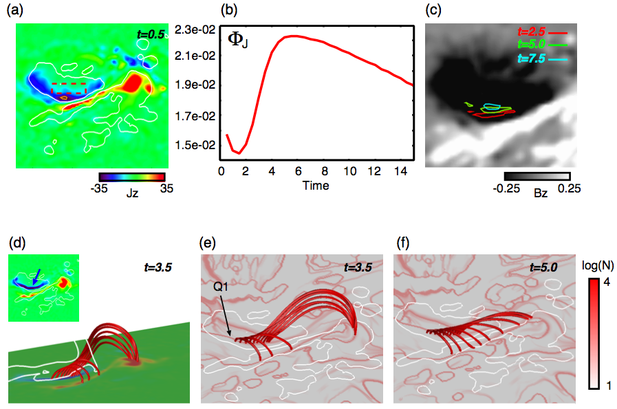
Figure 10: (a) A distribution of $J_{z}$ with contour of $|B_{z}|$=0.25 in white and $J_{z}$=$-$35 in orange at $t$=0.5. (b) Temporal evolution of the negative normal current flux, defined by $\int|-J_{z}|dS$, calculated in a region surrounded by red dashed square (0.433$<$x$<$0.49 and 0.533$<$y$<$0.567) marked in (a). (c) Temporal evolution of the contour for the $J_{z}$=$-$35, at $t$=2.5(in red), 5.0(in green), and 7.5(in aqua), respectively, on $B_{z}$ distribution. (d) The field lines are plotted in red, passing through the inside region surrounded by the contour of $|\mbox{\boldmath$J$}|$ = 10 over $J_{z}$ distributions. Insert is the top view of the $J_{z}$ map where the arrow points out the most enhanced region. (e)-(f) The field lines are plotted in the same format as (c) and are plotted with a distribution $N(x,y)$ defined in equation (11) at $t$=3.5 and $t$=5.0, respectively. The white contour represents the $|B_{z}|$=0.25.

Janvier et al. (2014) reported an enhancement of the normal current density ($J_{z}$) on the solar surface during the flare, particularly at the negative polarity in the central area (Region S- shown in Figure 3 in their paper). We also check the temporal evolution of the negative current density flux to compare with their observational result measured in the region S-. Figure 10(a) shows a distribution of $J_{z}$ at $t$=0.5 and orange line corresponds to a contour of $J_{z}$=-35 at which the $J_{z}$ is strongly enhanced. The normal current flux is measured in an area surrounded by red dashed square in Figure 10(a) which almost touches to the enhanced region of $J_{z}$ and close to the region S- set in Janvier et al. (2014). A temporal evolution of the negative normal current flux $\int|-J_{z}|dS$ is plotted in Figure 10(b). Our simulation results also shows its sudden enhancement, but its value decreases gradually after. This is different from the results found by Janvier et al. (2014) who observe a saturation of the normal current density. Figure 10(c) shows the temporal evolution of the contour for $J_{z}=-35$. This contour is moving away from the PIL as time progresses as shown in Aulanier et al. (2012), and the size becomes smaller as speculated in Figure 10(a).

We also checked the relationship between the enhanced current density and field line structure. The structure of field lines at $t$=3.5 passing through the inside of the current layer $|\mbox{\boldmath$J$}|=10$ is plotted in Figure 10(d). The one footpoint of these lines is rooted in the negative current region, where the current density is strongly enhanced. An insert exhibits the top view of the $J_{z}$ map at $t$=3.5 where the arrow points out the most enhanced region of the negative current density. We further calculate the norm to elucidate the property of these field lines. The norm is defined by following equation equation (Demoulin et al. 1996.)

$$N(x,y)=\sqrt{\sum_{i=1,2}\left[\left(\frac{\partial X_{i}}{\partial x}\right)^{2}+\left(\frac{\partial X_{i}}{\partial y}\right)^{2}\right]},$$ (11)

where $(X_{1},X_{2})$ is the relative distance corresponding to $(x^{\prime}-x^{\prime\prime},y^{\prime}-y^{\prime\prime})$. $(x^{\prime},y^{\prime})$ and $(x^{\prime\prime},y^{\prime\prime})$ are the positions of the end points of the field lines whose starting points are two adjacent grid points located at ($x^{\prime}_{0}$, $y^{\prime}_{0}$) and ($x^{\prime\prime}_{0}$, $y^{\prime\prime}_{0}$) on the photospheric surface. This means that the locations of the end points of these field lines, which are traced from these starting points across a large N(x,y) value, may differ greatly. Figure 10(e) plots the field lines at $t$=3.5. These are the same field lines as in Figure 10(d), with a distribution of N(x,y) added. We can clearly see that the one footpoint of these field lines is rooting into the enhanced negative current region and is across the N(x,y) marked by Q1. This means that the footpoints of the field lines in a different topology defined by N(x,y) coexist in the enhanced current layer. We further plot the field lines at $t$=5.0 in Figure 5(f), when all of field lines traced from the same location in Figure 10(e) become post-flare loops. From these results, the field liens plotted in Figure 10(d) or Figure 10(e) are in a sate just before and after the reconnection, and we found that the normal current density is strongly enhanced at the moment of reconnection, where the footpoint is rooted. These results are consistent with Janvier et al. (2013) demonstrating a relationship between the quasi separatrix layer (QSL) and current ribbons formed at the photosphere reproduced in their simulation.

In our simulation, the normal current flux cannot maintain the peaking value in its temporal evolution. This is in contrast to the observation made by Janvier et al. (2014). One possible reason for this difference might be related to our boundary condition arising from the initial NLFFF. The temporal evolution of the tangential fields in our simulation relaxes the shear gradually through the photosphere such that it trends toward the potential field or another low energy state gradually so that cannot trace the evolution as seen in the observation. Also the gap between the observation and simulation shown in Figure 9(e) might be caused by this problem. On the other hand, following Janvier et al. (2013), the current ribbons are linked with the current region in the solar corona at which the reconnection taking place, such that numerical diffusion might weaken this link.

4 Discussion

4.1 Change for the Connectivity in the Strongly Twisted Lines

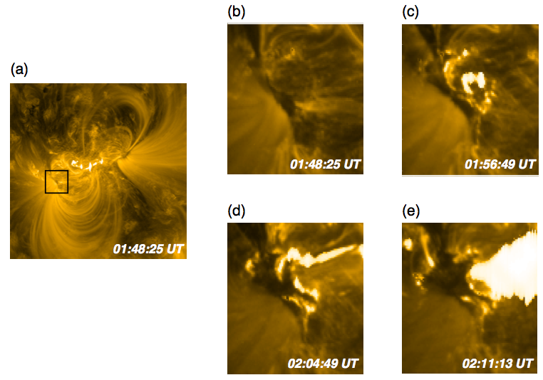
Figure 11: (a) EUV image taken from AIA 171 Å at 01:48:25 UT in the range of 216 $\times$ 216 $Mm^{2}$, corresponding to an area in which the NLFFF or MHD simulation is performed. (b)-(e) EUV images taken from AIA 171 Å from $t$= 01:48:25 to $t$=02:11:13 during the flare, in the range of a region surrounded by the black square in (a).

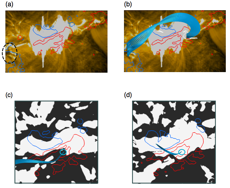
Figure 12: (a) EUV image taken by AIA 171 Å in the range of 0.25$<$x$<$0.78, 0.33$<$y$<$0.67 at 02:04:49UT. Red and blue lines correspond to the contours of $B_{z}$=0.25, and -0.25, respectively. (b) Field lines with more than a one-turn twist at $t$=15.0, i.e., flux tube, are plotted over (a). White line corresponds to the contour of $T_{n}$=1.0 at $t$=15.0 where the field lines are started from the inside of this region. (c) Map of open-closed field lines for the NLFFF on February 15 00:00UT corresponding to the 2 hours before the flare. White regions are dominated by the closed field lines where both footpoints are anchored in this field of view (FOV) (0.38$<$x$<$0.62, 0.4$<$y$<$0.63), while the black regions are dominated by the open magnetic field whose one footpoint goes through the boundary of this FOV. The blue lines are field lines traced from the solid circle. (d) Map of open-closed field lines for the NLFFF on February 15 03:00UT, corresponding to an hour after the flare. Figure format is same as in (c).

We found that one fooptpoint of the new large flux tube that had the strongly twisted lines and $T_{n}>$1.0 and was formed through reconnection during the flare was rooted into the negative polarity located southeast away from the central area as seen in Figures 7(d) or 8(b). We further check it by comparing it with another AIA images. Figure 11(a) exhibits the AIA 171 Å taken by the SDO at 01:48:25 UT on 2011 February 15, corresponding to the onset of the solar flare. The region surrounded by the black square corresponds to the area in which one footpoint of the flux tube was rooted during the flare, while another is rooted into the central area. The temporal evolutions of this area are shown in Figures 11(b)-(e). As time progresses during the flare, we can see that the dimming region is growing. Figure 12(a) shows another AIA image, taken during the middle flare phase and superimposed with $B_{z}$ contours. The black dashed circle corresponds to the region surrounded by the square marked in Figure 11(a). The strongly twisted field lines at $t$=15.0 are plotted in Figure 12(b), where these field lines are traced from the inside of the contour for the twist $T_{n}$=1.0 at $t$=15.0 in white on the positive polarity. We can see that another footpoint is rooted into the dimming region at the negative polarity, which is marked by the dashed circle in Figure 12(a).

Figures 12(c) and (d) map the distribution of the open-closed field lines obtained from the NLFFF before and after the flare, respectively, with the field lines traced by the blue solid circle. At the region marked by the blue circle in both panels, the open magnetic field lines going through the side or top boundaries of this field of view (FOV) dominate before the flare, while the closed field lines with both footpoints are anchored within this FOV dominate after the flare. Since this process implies the reconnection between the open and closed field lines and produces the large flux tube as shown in Figure 3, this might support the dynamics obtained from our MHD simulation.

4.2 A Relationship between 3D Dynamics and Enhancement of the Tangential Fields at the Solar Surface

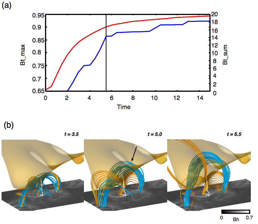
Figure 13: (a) A temporal evolution of the maximum value of the tangential components of the magnetic field, $B_{t_{max}}$, and its summation of that, $B_{t_{sum}}$ (=$\sum B_{t}$) where $B_{t}$ is counted over 0.8(=2000G), measured in the range of (0.25$L_{0}$ $<$x$<$ 0.75$L_{0}$, 0.25$L_{0}$ $<$y$<$ 0.75$L_{0}$) are plotted in red and blue, respectively. The vertical solid line indicates a location where the profile of the $B_{t_{sum}}$ suddenly changes from an increasing phase to the saturating phase. (b) Temporal evolution of the magnetic field lines with the contour of $|\mbox{\boldmath$J$}|=5.0$ in white and the isosurface of the threshold of the torus instability. Bottom surface represents the distribution of $B_{t}$. The blue field lines are drawn in the same format as in Figure 4, and orange field lines pass through the region surrounded by the contour of the current density in white. Arrow pointed out the intersection between the magnetic field lines and isosurface.

In section 3.4.1, we saw an enhancement of the tangential magnetic fields at the solar surface that reside close to the PIL. In this section, we explore a relationship between this enhancement and the structure seen in the 3D volume. We first plot the temporal evolution of the maximum value $B_{t_{max}}$ and summation ($B_{t_{sum}}$ (=$\sum B_{t}$)), for which the $B_{t}>$0.8 is counted, of the tangential magnetic fields in Figure 13(a). These values first increase during the initial flare phase (from $t$=0 to $t$=5.5), where the increasing ratio is 38$\%$ measured in $B_{t_{max}}$, but these values saturate approximately in the late phase, as seen by Wang et al. (2012). This transition might be explained by different 3D dynamics in the early and late flare phases. We therefore check the 3D magnetic structure to explain this transition.

Figure 13(b) shows the 3D view of the magnetic field at $t$=3.5, 5.0, and 6.5, respectively, with current density contours $|\mbox{\boldmath$J$}|=5.0$ and isosurfaces corresponding to the critical height of the torus instability. At $t$=3.5, when $B_{t_{max}}$ and $B_{t_{sum}}$ are increasing, the weakly twisted lines in blue which become the strongly twisted lines at $t$=6.5 are passing through the inside of the strong current region. This means that the large flux tube is forming in this phase through reconnection. At $t$=5.0 the large flux tube has been formed and its top is close to the location of the threshold of the torus instability. The profile of $B_{t_{max}}$ or $B_{t_{sum}}$ are just about to begin their saturation phase. Eventually, the large flux tube exceeds the threshold of the torus instability;then, $B_{t_{max}}$ or $B_{t_{sum}}$ remain in the saturation phase. These results imply the profile of $B_{t}$ shows two different picture in the formation of the large flux tube and its ascending phase over the threshold of the torus instability. The different 3D dynamics in the solar corona might be shown at the solar surface in the form of the enhancement of $B_{t}$.

Essentially, this would be controlled by the reconnection in the solar corona. In the earlier flare phase, the reconnection takes place in the lower corona, meaning that the magnetic field is reconnected effectively and can enhance the tangential magnetic field at the photosphere because the strong magnetic flux density exists there. On the other hand, at a later phase, the magnetic reconnection point shifts toward the higher coronal region associated with the rise of the flux tube, so the reconnection is not working effectively relative to the one in the lower corona, which might put the brake on the enhancement of the tangential fields at the photosphere. These more detailed and quantitative analyses not presented here are left as future work.

4.3 A Transition from Flare to CME

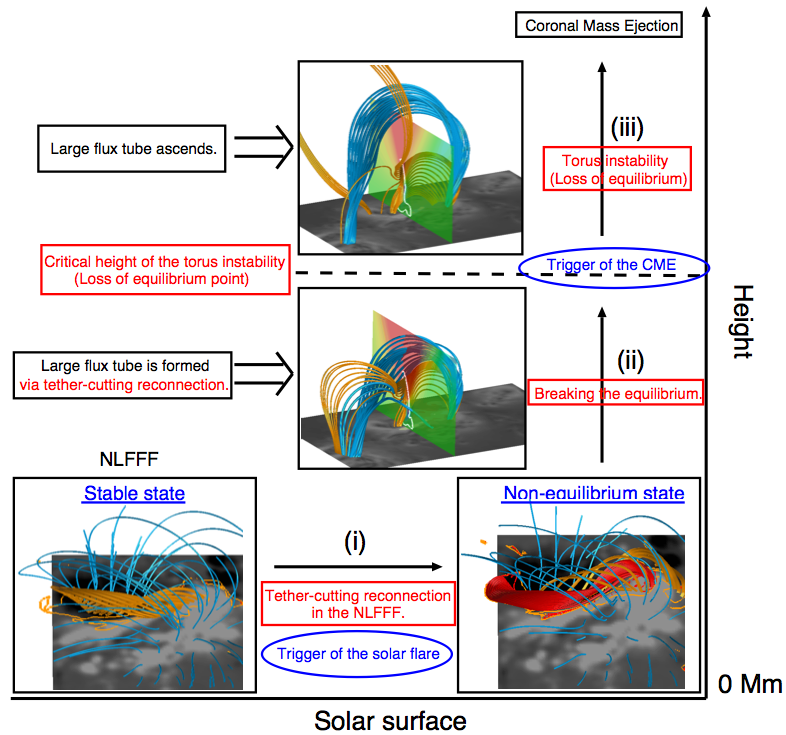
Figure 14: Summary of the dynamics in AR11158, based on our NLFFF extrapolations and MHD simulations. The upper two insets show the 3D structure of the field lines in the same format as in Figure 13(b), except that the vertical velocity is plotted on the vertical cross section, where its top corresponds to the approximate critical height of the torus instability.

Figure 14 shows a summary of the dynamics for the X2.2-class solar flare in AR11158 based on our simulation results. The onset of the solar flare starts in phase (i) where the strongly twisted lines are produced via tether-cutting reconnection of the twisted lines formed in the NLFFF. Consequently, the strongly twisted lines erupt away from the solar surface, and the sheared two-ribbon flares are appearing and new large flux tube is being formed in phase (ii). The CME onset starts in phase (iii), where the newly formed large flux tube is ascending upward over the threshold of the torus instability.

Inoue & Kusano (2006) suggested an existence of a critical height above which a flux tube cannot recover to the equilibrium state. They concluded that the CME formation due to the eruption in the flux tube is not enough to surpass the critical twist due to the kink instability;however, it is important to couple this with the loss of equilibrium such that the flux tube can grow over a certain height. Reaching the critical height of the torus instability would equate to the point where equilibrium is lost. In this study, the tether-cutting reconnection plays an important role as driver in the lower corona at the initial phase of flare-CME dynamics, rather than the kink instability. However, a scenario of the flare-CME relationship is basically the same as in our previous study Inoue & Kusano (2006).

5 Summary

We investigated the dynamics of the magnetic field during the X2.2-class solar flare taking place in AR11158, in particular focusing on the large flux tube formation and the related phenomena associated with the flares, eventually suggesting a relationship between flares and CMEs.

1. We first reconstruct the NLFFF based on the photospheric magnetic field prior to the X2.2-class solar flare in AR11158 on 2011 February 15. This NLFFF never showed the dramatic dynamics as seen in observations because it is stable even against small perturbations (see Inoue et al. 2014a), i.e., it is stable against the ideal MHD instability such as like kink and torus instabilities. The NLFFF, therefore, needs to be excited into higher energy levels to cause the huge flares.

2. We further performed the MHD relaxation, i.e., the MHD simulation with the fixed boundary condition where the three components of the magnetic field are fixed at the bottom surface, using the NLFFF as an initial condition. An anomalous resistivity is applied in this calculation and as a result, the strongly twisted lines are produced through the reconnection between twisted lines taking place in the strong current region formed in the NLFFF. Because this magnetic configuration cannot keep the equilibrium state, the strongly twisted lines successfully showed the eruption due to a loss of equilibrium. In fact, the same kinds of trigger processes are needed, rather than the anomalous resistivity, to produce the strongly twisted lines through the tether-cutting reconnection and bring them up to a critical height of the torus instability. We here point out some pioneering works about the triggering process of the solar flare: Flux cancellation on the photosphere (van Ballegooijen & Martens 1989; Green et al. 2011; Amari et al. 2010; Amari et al. 2011), emerging magnetic flux through the photosphere (Heyvaerts et al. 1977; Feynman & Martin 1995; Chen & Shibata 2000; Roussev et al. 2012; Kusano et al. 2012; Toriumi et al. 2013; Bamba et al. 2013). These processes should be taken in account in our simulation as important future work so that our model does not depend on the anomalous resistivity model.

3. Although the strongly twisted lines with more than a one-turn twist launch away from the solar surface, they further reconnected with the ambient weakly twisted lines. Consequently, the new large flux tube is formed. This result shows that the large flux tube growing into the CME is formed through the tether-cutting reconnection between the strongly and weakly twisted lines. The tether-cutting reconnection, therefore, plays an important role in the triggering process of the CME, i.e., the formation process of the large flux tube and overcoming the threshold of the torus instability, as well as the triggering process of the flare, i.e., the formation of the strongly twisted lines in the NLFFF driving the initial eruption. Our results suggested that the flare and CME are connected via these two scenarios.

4. We investigated a relationship between the distribution of $\Delta$ defined in equation (10), corresponding to the connectivity change of a twisted field line, and the distribution of the twisted lines. This $\Delta$ distribution well resembles the distribution of the observed two-ribbon flare in the earlier flare phase. Most of the strong $\Delta$ region is found just outside of the region of the strongly twisted magnetic field. On the other hand, we found that the footpoint of the long twisted lines is anchored into the hook area formed in the $\Delta$ distribution surrounding the footpoint of the eruptive strongly twisted lines. This scenario would be similar to the 3D flare model in Aulanier et al. (2012) and Janvier et al. (2013). However, following this point, the eruptive strongly twisted lines showed complicated behaviors, in particular, the reconnection between the strongly and weakly twisted lines resulting from the complex magnetic topology of AR 11158, through which the large flux tube is formed as mentioned above.

5. In our simulation, we observed a portion of the tangential magnetic field, $B_{t}$ at the solar surface residing close to the PIL in the earlier flare phase, whose maximum value was recorded to be more than 2000 G. During this phase, the dynamics of the twisted lines are observed within a region less than the critical height of the torus instability in which the large flux tube formation is beginning. We further found that the post-flare loops already exist and cover the region on the photosphere where $B_{t}$ is enhanced, even though the shear angle between the tangential components in the simulation and that of the potential fields decreases there gradually with time. Therefore, this enhancement is inferred due to be piled up by the new post-flare loops produced by the sequential reconnection, i.e., $B_{t}$ on the photosphere is compressed by them and then enhanced. After the large flux tube forms and exceeds a critical height of the torus instability, the value of $B_{t}$ approximately reaches saturation. The maximum value increases 38$\%$ during the initial flare phase while Wang et al. (2012) reports the average value at the selected region increases by $\sim$ 30$\%$. These results indicate the different profile of $B_{t}$ on the photosphere, such that increasing or saturating behaviors might be projected by the different 3D dynamics observed in the solar corona. On the other hand, although Wang et al. (2012) and Sun et al. (2012) pointed out the tangential fields become better aligned with the PIL during the flare, these ’more parallel field lines’ appearing in the lowest area were not reproduced in our simulation.

6. We also found the enhancement of $J_{z}$ on the solar surface in our MHD simulation, which is consistent with the analysis of the observed result by Janvier et al. (2014). This enhancement is observed in a region where a footpoint of the field lines in which reconnection is taking place in the strong current region is rooted, as pointed out by Janvier et al. (2013). On the other hand, our MHD simulation showed that the value of $J_{z}$ is decreasing gradually as time passes after its enhancement, which is different from the observed picture. There are still some gaps which remain between the observations and simulation.

In this paper we investigate the dynamics of magnetic fields during the X2.2-class flare taking place in AR11158, focusing in particular on the transition dynamics from the solar flare to the CME. Unfortunately, we cannot trace the evolution of the flux tube for a long enough time within the limited volume of the simulation, i.e., we cannot conclude whether or not the large flux tube shown in our MHD simulation is in its final form. Hu et al. (2014) reported a very highly twist flux tube traveling an interplanetary, up to 5 turns per AU, which decreases toward the edge. At least, our NLFFF or flux tube just launching from the solar surface whose twist values are concentrated mostly in a range from one turn to 1.5 turns cannot explain this highly twist. Yamamoto et al. (2010) also made an effort to clear the gap of twist between measured at the solar surface and interplanetary. But the problem has been left yet. A large-scale simulation covering the interplanetary space would be important to fill this gap.

On the other hand, the twist accumulated in the large flux tube looks weak compared to the initial twisted lines in red in Figure 3(a) even though the flux tube exceeds a one-turn twist. These would be caused by two problems: one is due to a numerical diffusion (Su et al. 2011); another is due to the initial NLFFF. In order to settle these problems, a high-resolution simulation is important to suppress the numerical diffusion, i.e., suppress the diffusion of the twist accumulated in the flux tube. Furthermore, a higher accurate NLFFF, achieving more close to an equilibrium state, would be also required to avoid release of a shear through the boundary. These problems must be settled to complete the data-constrained or -driven simulation for solar flares and CMEs. On the other hand, future observations plan to observe a chromospheric magnetic field (e.g., SOLAR-C mission Watanabe 2014). Because a chromospheric magnetic field is in a lower $\beta$ state than that of the photospheric magnetic field, it would help us definitely construct higher accurate NLFFFs and perform data-constrained or -driven simulations.

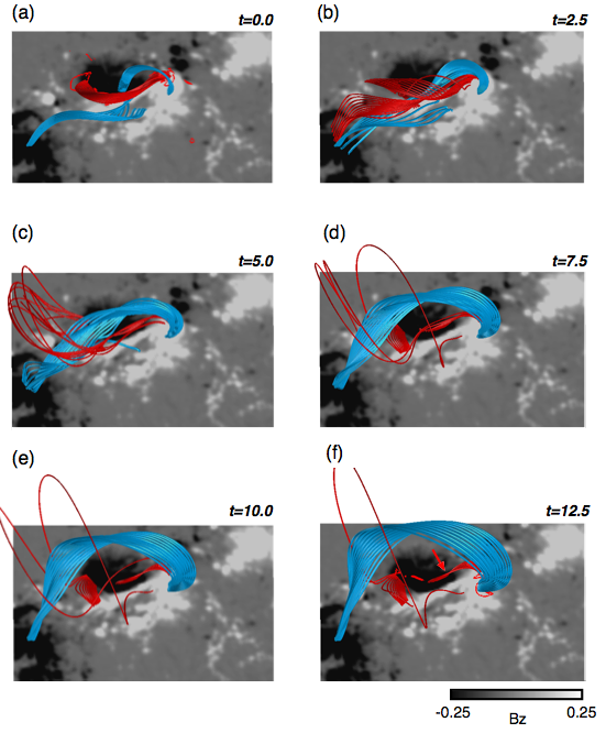
Figure 3: Temporal evolution of the dynamics of the selected magnetic field lines with $B_{z}$ distribution. The red and blue lines represent the field lines more and less than a one-turn twist, respectively, at an initial time $t$=0.0. Note that most of the blue lines have weak twist less than 0.35 turns. The red arrow indicates sheared-post flare loops. The contour of $T_{n}$=1.0 is plotted at surface in red at $t$=0.0 and 12.5.

References

- Amari et al. (1996) Amari, T., Luciani, J. F., Aly, J. J., & Tagger, M. 1996, ApJ, 466, L39
- Amari et al. (2000) Amari, T., Luciani, J. F., Mikic, Z., & Linker, J. 2000, ApJ, 529, L49
- Amari et al. (2003) Amari, T., Luciani, J. F., Aly, J. J., Mikic, Z., & Linker, J. 2003, ApJ, 585, 1073
- Amari et al. (2010) Amari, T., Aly, J.-J., Mikic, Z., & Linker, J. 2010, ApJ, 717, L26
- Amari et al. (2011) Amari, T., Aly, J.-J., Luciani, J.-F., Mikic, Z., & Linker, J. 2011, ApJ, 742, L27
- An & Magara (2013) An, J. M., & Magara, T. 2013, ApJ, 773, 21
- Antiochos et al. (1999) Antiochos, S. K., DeVore, C. R., & Klimchuk, J. A. 1999, ApJ, 510, 485
- Aulanier et al. (2010) Aulanier, G., Török, T., Démoulin, P., & DeLuca, E. E. 2010, ApJ, 708, 314
- Aulanier et al. (2012) Aulanier, G., Janvier, M., & Schmieder, B. 2012, A&A, 543, A110
- Bamba et al. (2013) Bamba, Y., Kusano, K., Yamamoto, T. T., & Okamoto, T. J. 2013, ApJ, 778, 48
- Berger & Prior (2006) Berger, M. A., & Prior, C. 2006, Journal of Physics A Mathematical General, 39, 8321
- Benz (2008) Benz, A. O. 2008, Living Reviews in Solar Physics, 5, 1
- Bobra et al. (2014) Bobra, M. G., Sun, X., Hoeksema, J. T., et al. 2014, Sol. Phys., 289, 3549
- Borrero et al. (2011) Borrero, J. M., Tomczyk, S., Kubo, M., et al. 2011, Sol. Phys., 273, 267
- Canou & Amari (2010) Canou, A., & Amari, T. 2010, ApJ, 715, 1566
- Carmichael (1964) Carmichael, H. 1964, NASA, Special Pub., 50, 451
- Carrington (1859) Carrington, R. C. 1859, MNRAS, 20, 13
- Demoulin et al. (1996) Demoulin, P., Henoux, J. C., Priest, E. R., & Mandrini, C. H. 1996, A&A, 308, 643
- Chen & Shibata (2000) Chen, P. F., & Shibata, K. 2000, ApJ, 545, 524
- Cheng et al. (2014) Cheng, X., Ding, M. D., Zhang, J., et al. 2014, ApJ, 789, 93
- De Rosa et al. (2009) De Rosa, M. L., Schrijver, C. J., Barnes, G., et al. 2009, ApJ, 696, 1780
- Fan (2010) Fan, Y. 2010, ApJ, 719, 728
- Fan & Gibson (2007) Fan, Y., & Gibson, S. E. 2007, ApJ, 668, 1232
- Feynman & Martin (1995) Feynman, J., & Martin, S. F. 1995, J. Geophys. Res., 100, 3355
- Forbes (1990) Forbes, T. G. 1990, J. Geophys. Res., 95, 11919
- Forbes (2000) Forbes, T. G. 2000, J. Geophys. Res., 105, 23153
- Green et al. (2011) Green, L. M., Kliem, B., & Wallace, A. J. 2011, A&A, 526, A2
- He et al. (2014) He, H., Wang, H., Yan, Y., Chen, P. F., & Fang, C. 2014, Journal of Geophysical Research (Space Physics), 119, 3286
- Heyvaerts et al. (1977) Heyvaerts, J., Priest, E. R., & Rust, D. M. 1977, ApJ, 216, 123
- Hirayama (1974) Hirayama, T. 1974, Sol. Phys., 34, 323
- Hoeksema et al. (2014) Hoeksema, J. T., Liu, Y., Hayashi, K., et al. 2014, Sol. Phys., 289, 3483
- Hu et al. (2014) Hu, Q., Qiu, J., Dasgupta, B., Khare, A., & Webb, G. M. 2014, ApJ, 793, 53
- Inoue & Kusano (2006) Inoue, S., & Kusano, K. 2006, ApJ, 645, 742
- Inoue et al. (2011) Inoue, S., Kusano, K., Magara, T., Shiota, D., & Yamamoto, T. T. 2011, ApJ, 738, 161
- Inoue et al. (2012) Inoue, S., Shiota, D., Yamamoto, T. T., et al. 2012, ApJ, 760, 17
- Inoue et al. (2013) Inoue, S., Hayashi, K., Shiota, D., Magara, T., & Choe, G. S. 2013, ApJ, 770, 79
- Inoue et al. (2014b) Inoue, S., Magara, T., Pandey, V. S., et al. 2014b, ApJ, 780, 101
- Inoue et al. (2014a) Inoue, S., Hayashi, K., Magara, T., Choe, G. S., & Park, Y. D. 2014a, ApJ, 788, 182
- Janvier et al. (2013) Janvier, M., Aulanier, G., Pariat, E., & Démoulin, P. 2013, A&A, 555, A77
- Janvier et al. (2014) Janvier, M., Aulanier, G., Bommier, V., et al. 2014, ApJ, 788, 60
- Jiang et al. (2013) Jiang, C., Feng, X., Wu, S. T., & Hu, Q. 2013, ApJ, 771, L30
- Jiang et al. (2014) Jiang, C., Wu, S. T., Feng, X., & Hu, Q. 2014, ApJ, 780, 55
- Karpen et al. (2012) Karpen, J. T., Antiochos, S. K., & DeVore, C. R. 2012, ApJ, 760, 81
- Kliem & Török (2006) Kliem, B., Török, T. 2006, Physical Review Letters, 96, 255002
- Kliem et al. (2013) Kliem, B., Su, Y. N., van Ballegooijen, A. A., & DeLuca, E. E. 2013, ApJ, 779, 129
- Kopp & Pneuman (1976) Kopp, R. A., & Pneuman, G. W. 1976, Sol. Phys., 50, 85
- Kosugi et al. (2007) Kosugi, T., Matsuzaki, K., Sakao, T., et al. 2007, Sol. Phys., 243, 3
- Kusano et al. (2012) Kusano, K., Bamba, Y., Yamamoto, T. T., et al. 2012, ApJ, 760, 31
- Leake et al. (2014) Leake, J. E., Linton, M. G., & Antiochos, S. K. 2014, ApJ, 787, 46
- Leka et al. (2009) Leka, K. D., Barnes, G., Crouch, A. D., et al. 2009, Sol. Phys., 260, 83
- Lemen et al. (2012) Lemen, J. R., Title, A. M., Akin, D. J., et al. 2012, Sol. Phys., 275, 17
- Lynch et al. (2008) Lynch, B. J., Antiochos, S. K., DeVore, C. R., Luhmann, J. G., & Zurbuchen, T. H. 2008, ApJ, 683, 1192
- Magara (2013) Magara, T. 2013, PASJ, 65, L5
- Masuda et al. (1994) Masuda, S., Kosugi, T., Hara, H., Tsuneta, S., & Ogawara, Y. 1994, Nature, 371, 495
- Metcalf (1994) Metcalf, T. R. 1994, Sol. Phys., 155, 235
- Moore et al. (2001) Moore, R. L., Sterling, A. C., Hudson, H. S., & Lemen, J. R. 2001, ApJ, 552, 833
- Pagano et al. (2013) Pagano, P., Mackay, D. H., & Poedts, S. 2013, A&A, 554, A77
- Pesnell et al. (2012) Pesnell, W. D., Thompson, B. J., & Chamberlin, P. C. 2012, Sol. Phys., 275, 3
- Priest & Forbes (2002) Priest, E. R., & Forbes, T. G. 2002, A&A Rev., 10, 313
- Régnier (2013) Régnier, S. 2013, Sol. Phys., 288, 481
- Régnier & Amari (2004) Régnier, S., & Amari, T. 2004, A&A, 425, 345
- Roussev et al. (2012) Roussev, I. I., Galsgaard, K., Downs, C., et al. 2012, Nature Physics, 8, 845
- Sakurai (1982) Sakurai, T. 1982, Sol. Phys., 76, 301
- Scherrer et al. (2012) Scherrer, P. H., Schou, J., Bush, R. I., et al. 2012, Sol. Phys., 275, 207
- Schrijver et al. (2011) Schrijver, C. J., Aulanier, G., Title, A. M., Pariat, E., & Delannée, C. 2011, ApJ, 738, 167
- Shibata & Magara (2011) Shibata, K., & Magara, T. 2011, Living Reviews in Solar Physics, 8, 6
- Schrijver et al. (2008) Schrijver, C. J., DeRosa, M. L., Metcalf, T., et al. 2008, ApJ, 675, 1637
- Sturrock (1966) Sturrock, P. A. 1966, Nature, 211, 695
- Su et al. (2007) Su, Y., Golub, L., & Van Ballegooijen, A. A. 2007, ApJ, 655, 606
- Su et al. (2011) Su, Y., Surges, V., van Ballegooijen, A., DeLuca, E., & Golub, L. 2011, ApJ, 734, 53
- Sun et al. (2012) Sun, X., Hoeksema, J. T., Liu, Y., et al. 2012, ApJ, 748, 77
- Thalmann & Wiegelmann (2008) Thalmann, J. K., & Wiegelmann, T. 2008, A&A, 484, 495
- Toriumi et al. (2013) Toriumi, S., Iida, Y., Bamba, Y., et al. 2013, ApJ, 773, 128
- Török & Kliem (2005) Török, T., & Kliem, B. 2005, ApJ, 630, L97
- Török et al. (2010) Török, T., Berger, M. A., & Kliem, B. 2010, A&A, 516, A49
- Török & Kliem (2007) Török, T., & Kliem, B. 2007, Astronomische Nachrichten, 328, 743
- Tsuneta et al. (1992) Tsuneta, S., Hara, H., Shimizu, T., et al. 1992, PASJ, 44, L63
- Tsuneta et al. (2008) Tsuneta, S., Ichimoto, K., Katsukawa, Y., et al. 2008, Sol. Phys., 249, 167
- van Ballegooijen & Martens (1989) van Ballegooijen, A. A., & Martens, P. C. H. 1989, ApJ, 343, 971
- van Driel-Gesztelyi et al. (2014) van Driel-Gesztelyi, L., Baker, D., Török, T., et al. 2014, ApJ, 788, 85
- Wang et al. (2012) Wang, S., Liu, C., Liu, R., et al. 2012, ApJ, 745, L17
- Watanabe (2014) Watanabe, T. 2014, Proc. SPIE, 9143, 91431O
- Wiegelmann & Sakurai (2012) Wiegelmann, T., & Sakurai, T. 2012, Living Reviews in Solar Physics, 9, 5
- Wiegelmann et al. (2006) Wiegelmann, T., Inhester, B., & Sakurai, T. 2006, Sol. Phys., 233, 215
- Yamamoto et al. (2010) Yamamoto, T. T., Kataoka, R., & Inoue, S. 2010, ApJ, 710, 456
- Yokoyama et al. (2001) Yokoyama, T., Akita, K., Morimoto, T., Inoue, K., & Newmark, J. 2001, ApJ, 546, L69
- Zuccarello et al. (2012) Zuccarello, F. P., Meliani, Z., & Poedts, S. 2012, ApJ, 758, 117