The QCD Equation of State

Abstract:

Results for the equation of state in 2+1 flavor QCD at zero net baryon density using the Highly Improved Staggered Quark (HISQ) action by the HotQCD collaboration are presented. The strange quark mass was tuned to its physical value and the light (up/down) quark masses fixed to $m_{l}=0.05m_{s}$ corresponding to a pion mass of 160 MeV in the continuum limit. Lattices with temporal extent $N_{t}=6$, 8, 10 and 12 were used. Since the cutoff effects for $N_{t}>6$ were observed to be small, reliable continuum extrapolations of the lattice data for the phenomenologically interesting temperatures range $130\mathord{\rm MeV}<T<400\mathord{\rm MeV}$ could be performed. We discuss statistical and systematic errors and compare our results with other published works.

1 Introduction

Hadronic matter deconfines at temperatures above $155~{}\mathord{\hbox{MeV}}$, where quark and gluons constitute the relevant degrees of freedon. Nevertheless, the theory remains non-perturbative because of the strongly interacting infrared sector, and the equation of state (EOS) of this quark-gluon plasma requires non-perturbative analysis using methods such as lattice QCD. The EOS is needed in modeling the hydrodynamic evolution of the quark-gluon plasma probed in relativistic heavy-ion collisions and in understanding the cooling of the early universe. Phenomenologically, the most interesting region for lattice QCD analysis is between $T\ sim140$ MeV and $400~{}\mathord{\hbox{MeV}}$, i.e., above the validity of hadron-resonance gas models and spanning the temperatures probed in relativistic heavy-ion collisions including the ‘transition’ region around $154(9)~{}\mathord{\hbox{MeV}}$ [1].

2 Lattice Details and the Trace Anomaly

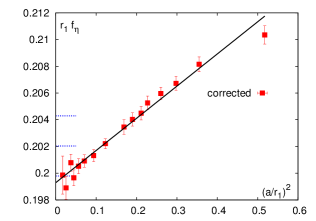
white	white
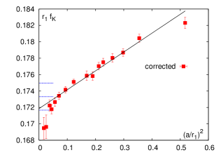
(a)	(b)
white	white
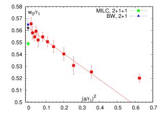
(c)	(d)

Figure 1: The continuum estrapolation of (a) $r_{1}f_{\eta}$, (b) $r_{1}f_{K}$, (c) $r_{1}M_{\phi}$ and (d) $w_{0}/r_{1}$, along with their continuum values [2, 3]. The data have been corrected for the mass mistuning described later in the text.

We summarize the calculation of EOS [4] by the HotQCD collaboration using $2+1$ flavors of fermions with the HISQ/tree action. In this calculation, we varied $\beta=10/g^{2}$ in the interval $5.9$–$7.825$ along a line of constant physics (LoCP) defined by the $s\overline{s}$ meson mass tuned to $M_{s\overline{s}}\approx 695~{}\mathord{\hbox{MeV}}$ and the light quark mass fixed at $m_{l}=m_{s}/20$ ($M_{\pi}\approx 160~{}\mathord{\hbox{MeV}}$), as used in our previous calculation [1]. To control discretization effects, the calculation was done at four values of the temporal size $N_{\tau}=6$, $8$, $10$, and $12$. The spatial size was fixed at 4 times $N_{\tau}$, i.e., $N_{\sigma}/N_{\tau}=4$. The lattice update was done with the RHMC algorithm with mass preconditioning [5]. All the results are reported with the lattice scale set by $r_{1}=0.3106(14)(8)(4)~{}\mathord{\hbox{fm}}$ [6]. We checked that in our calculation this corresponded to $r_{0}=0.4688(41)~{}\mathord{\hbox{fm}}$ and $w_{0}=0.1749(14)~{}\mathord{\hbox{fm}}$ consistent with the previous determinations $0.48(1)(1)~{}\mathord{\hbox{fm}}$ [7] and $0.1755(18)(4)~{}\mathord{\hbox{fm}}$ [8] respectively. This estimate is also consistent, in the continuum limit, with the scale obtained from various fermionic quantities as shown in Fig. 1.

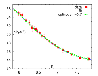
white	white
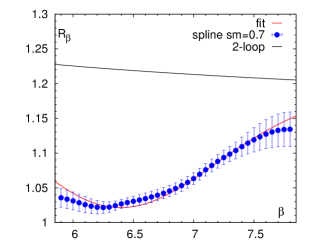
(a)	(b)

Figure 2: (a) The scale, $a/r_{1}$, normalized by the two-loop beta function, $f(\beta)$, showing a fit and a spline interpolation to the data and (b) the non-perturbative $\beta$-function, $R_{\beta}$, compared to the two-loop value.

After integrating out the fermion degrees of freedom, the QCD partition function on an $N_{\sigma}^{3}N_{\tau}$ hypercubic lattice can be written as

$$Z(\beta,N_{\sigma},N_{\tau})=\int\prod_{x,\mu}dU_{x,\mu}e^{-(\beta\,S_{G}(U)-S_{F}(U))}\,,$$ (1)

where $s_{G}(U)$ and $s_{F}(U)$ are the gauge and fermionic actions in terms of the $\mathord{\hbox{SU(3)}}$ link variables $U$. From this we can calculate the energy density, $\varepsilon$, and pressure, $p$, in terms of the temperature, $T$, starting with the trace anomaly, $\Theta^{\mu\mu}$ and using the relations

$$T\frac{d}{dT}\left(\frac{p}{T^{4}}\right) = \frac{\varepsilon-3p}{T^{4}}\;=\;\frac{\Theta^{\mu\mu}_{G}(T)}{T^{4}}+\frac{\Theta^{\mu\mu}_{F}(T)}{T^{4}}\,,$$ (2)

$$\frac{\Theta^{\mu\mu}_{G}(T)}{T^{4}} = R_{\beta}\left[\langle s_{G}\rangle_{0}-\langle s_{G}\rangle_{\tau}\right]N_{\tau}^{4}\,,$$ (3)

$$\frac{\Theta^{\mu\mu}_{F}(T)}{T^{4}} = -R_{\beta}R_{m}\left[2m_{l}\left(\langle\bar{\psi}\psi\rangle_{l,0}-\langle\bar{\psi}\psi\rangle_{l,\tau}\right)+m_{s}\left(\langle\bar{\psi}\psi\rangle_{s,0}-\langle\bar{\psi}\psi\rangle_{s,\tau}\right)\right]N_{\tau}^{4}\,,$$ (4)

where the subscripts $\tau$ and $0$ refer to expectation values at finite and zero temperature respectively, and $l$ and $s$ refer to the light and strange quark condensates, respectively. The function $R_{\beta}$ is the non-perturbative $\beta$ function,

$$R_{\beta}(\beta)=\frac{r_{1}}{a}\left(\frac{{\rm d}(r_{1}/a)}{{\rm d}\beta}\right)^{-1}$$ (5)

shown in Fig. 2 and $R_{m}$ is the mass renormalization function,

$$R_{m}(\beta)=\frac{1}{m_{s}(\beta)}\frac{{\rm d}m_{s}(\beta)}{{\rm d}\beta}\,.$$ (6)

Since the measured value of $M_{s\bar{s}}$ has small deviations from LoCP, as shown in Fig. 3(a), we corrected it using lowest order chiral perturbation theory. The corrected mass parameter used in the analysis and to obtain $R_{m}$ is shown in Fig. 3(b).

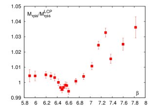
white	white
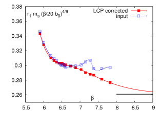
(a)	(b)

Figure 3: (a) The measured value of $M_{\eta}^{ss}$ normalized by $695~{}\mathord{\hbox{MeV}}$ showing a few percent mistuning at higher $\beta$. (b) The one-loop renormalization-group-invariant strange-quark mass in units of $r_{1}^{-1}$, and the same after correcting for the mistuning, along with a spline interpolation and the asymptotic value at infinite $\beta$.

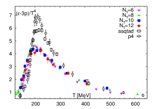
white	white
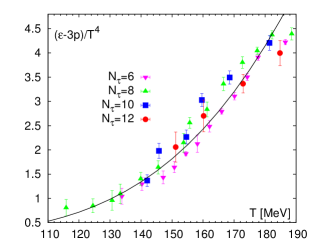
(a)	(b)

Figure 4: (a) The trace anomaly calculated at four different $N_{\tau}$ compared to our previous calculations [9, 10, 11]. (b) A magnification of the low temperature region with the results from a HRG model including all hadrons in the Particle Data Book [3] with masses less than $2.5~{}\mathord{\hbox{GeV}}$ shown as a solid line.

All our data for the trace anomaly are shown in Fig. 4(a) and compared to our previous calculations using the p4 and asqtad lattice actions. The noticeable difference is that the peak in the HISQ/tree data is lower and shifted to the left. In Fig. 4(b), we show that the results for $T\lesssim 145~{}\mathord{\hbox{MeV}}$ at different $N_{\tau}$ are consistent and agree with those obtained using the hadron resonance gas (HRG) model.

3 Continuum Extrapolation

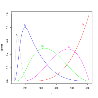
white	white
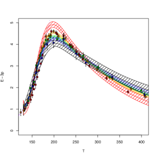
(a)	(b)

Figure 5: (a) A B-spline basis with two internal knots that are constrained to go to zero at $130~{}\rm{MeV}$. (b) The extrapolation of the lattice data at $N_{\tau}=8$, $10$ and $12$ to the continuum is shown as a black band. The fit results at the various $N_{\tau}$ are shown as colored bands.

The quality of the lattice data is sufficiently good that various strategies for extrapolating them to the continuum limit agree within errors. The one with least free parameters is a simultaneous fit that interpolates the data in $T$ and extrapolates in $1/N_{\tau}^{2}\to 0$. This is implemented by choosing a basis of cubic splines that enforces the continuity of the function along with its first and second derivatives in $T$. An example of a B-spline basis with two knots is shown in Fig. 5(a).

We explore fits with coefficients of the basis functions chosen as linear or quadratic functions of $1/N_{\tau}^{2}$, thus enforcing the same continuity requirements on the extrapolation. To stabilize our fits, we match the value and the first temperature-derivative of the continuum extrapolated value on to the HRG results at $T=130~{}\mathord{\hbox{MeV}}$. Since with $n$ internal knots, the B-spline basis has $n+4$ basis elements, the HRG condition at 130 MeV reduces the number of continuum coefficients to $n+2$. For the extrapolation linear in $1/N_{\tau}^{2}$, we have an additional $n+4$ coefficients and the choice of $n$ knot positions, for a total of $3n+6$ degrees of freedom (d.o.f). The fit was performed by minimizing the uncorrelated $\chi^{2}$ and $n$ was chosen according to the Akaike Information Criterion (AIC) of minimizing $\chi^{2}+2\times\mathord{\hbox{d.o.f}}$. All the calculations were done using the statistical program R [12] and its Hmisc package [13].

To estimate the errors in the fit parameters, we generated 20,001 synthetic data sets drawn assuming a normal distribution with variance given by the estimated error on each measurement. We assigned an independent conservative 10% error on both the value and slope of the HRG at $T=130~{}\mathord{\hbox{MeV}}$. To the bootstrap error we linearly added a 2% error to account for scale uncertainty in determining $T$.

An extrapolation ansatz just linear in $1/N_{\tau}^{2}$ does not fit the $N_{\tau}=6$ data well. Our best estimate is obtained using a fit with 2 knots and linear in $1/N_{\tau}^{2}$ to the $N_{\tau}=8$, $10$ and $12$ data at $T\lesssim 400~{}\mathord{\hbox{MeV}}$. To stabilize the fit at the upper end, we included the $N_{\tau}=8$ data up to $T=610~{}\mathord{\hbox{MeV}}$. This final extrapolation is shown in Fig. 5(b).

4 Results and Conclusions

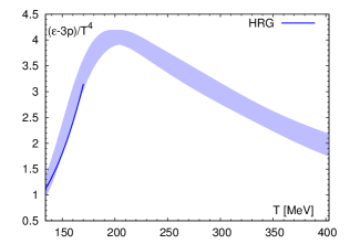
white	white
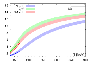
(a)	(b)

Figure 6: (a) The continuum extrapolated integration measure (band) compared to the HRG estimate (solid line). (b) The continuum extrapolated pressure, $p$, energy density, $\varepsilon$, and entropy density, $s$, (colored bands) compared to the HRG estimate (colored solid lines) and the Stephan-Boltzman value (solid black line) for an ideal gas.

As shown in Fig. 6, our extrapolated continuum results for the integration measure, pressure, energy density and the entropy density agree in value with the HRG estimates for $T\lesssim 150~{}\mathord{\hbox{MeV}}$. The speed of sound and the specific heat shown in 7(b,c), which depend on higher derivatives of the partition function, are, however, not well predicted by this model. Figs. 6(b) and 7(c) also show that the quark-gluon plasma is still significantly far from a non-interacting gas even at $T\approx 400~{}\mathord{\hbox{MeV}}$.

In Fig. 7(a) and (b) we comapre our results with those by the Wuppertal-Budapest collaboration using a stout dicretization of the fermion action [14] and find good agreement. There may be a small discrepancy for $T>350~{}\mathord{\hbox{MeV}}$ which is probably unimportant for current heavy ion phenomenology, but needs further investigation to study the approach to the high temperature perturbative regime. Lastly, the disagreements with our previous results for the EOS using the p4 and asqtad actions were due to large cutoff effects in those calculations.

white
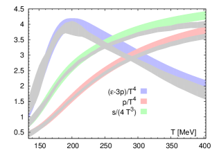
(a)
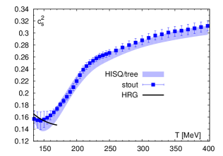
white	white
(b)	(c)

Figure 7: (a) Comparison of our results for pressure, $p$, energy density, $\varepsilon$, and entropy density, $s$, (colored bands) with the results from the Wuppertal-Budapest collaboration using the stout discretization [14] (grey bands). (b) Our results for the speed of sound, $c_{s}$ (colored band) compared to the stout results (data points) and the HRG estimate (black solid line). (c) Our results for the specific heat, $C_{V}$, (colored band) compared to the HRG results (colored line) and the value for a non-interacting gas (horizontal black line). Also shown is the result from a parameterization designed to the fit the pressure and energy density (black curve).

References

- [1] A. Bazavov, T. Bhattacharya, M. Cheng, C. DeTar, H.T. Ding, et al. Phys.Rev., D85:054503, 2012, doi:10.1103/PhysRevD.85.054503, arXiv:1111.1710.
- [2] C.T.H. Davies, E. Follana, I.D. Kendall, G. Peter Lepage, and C. McNeile, HPQCD Collaboration. Phys.Rev., D81:034506, 2010, doi:10.1103/PhysRevD.81.034506, arXiv:0910.1229.
- [3] J. Beringer et al., Particle Data Group. Phys.Rev., D86:010001, 2012, doi:10.1103/PhysRevD.86.010001.
- [4] A. Bazavov et al., HotQCD Collaboration. Phys.Rev., D90(9):094503, 2014, doi:10.1103/PhysRevD.90.094503, arXiv:1407.6387.
- [5] M.A. Clark, Ph. de Forcrand, and A.D. Kennedy. PoS, LAT2005:115, 2006, arXiv:hep-lat/0510004.
- [6] A. Bazavov et al., MILC Collaboration. PoS, LATTICE2010:074, 2010, arXiv:1012.0868.
- [7] Y. Aoki, Szabolcs Borsanyi, Stephan Durr, Zoltan Fodor, Sandor D. Katz, et al. JHEP, 0906:088, 2009, doi:10.1088/1126-6708/2009/06/088, arXiv:0903.4155.
- [8] Szabolcs Borsanyi, Stephan Durr, Zoltan Fodor, Christian Hoelbling, Sandor D. Katz, et al. JHEP, 1209:010, 2012, doi:10.1007/JHEP09(2012)010, arXiv:1203.4469.
- [9] M. Cheng, N.H. Christ, S. Datta, J. van der Heide, C. Jung, et al. Phys.Rev., D77:014511, 2008, doi:10.1103/PhysRevD.77.014511, arXiv:0710.0354.
- [10] A. Bazavov, T. Bhattacharya, M. Cheng, N.H. Christ, C. DeTar, et al. Phys.Rev., D80:014504, 2009, doi:10.1103/PhysRevD.80.014504, arXiv:0903.4379.
- [11] P. Petreczky. Nucl.Phys., A830:11C–18C, 2009, doi:10.1016/j.nuclphysa.2009.10.086, arXiv:0908.1917.
- [12] R Core Team. R Foundation for Statistical Computing, Vienna, Austria, 2014, url:http://www.R-project.org/.
- [13] Frank E Harrell Jr, with contributions from Charles Dupont, and many others. 2014, url:http://CRAN.R-project.org/package=Hmisc. R package version 3.14-4.
- [14] Szabocls Borsanyi, Zoltan Fodor, Christian Hoelbling, Sandor D. Katz, Stefan Krieg, et al. Phys.Lett., B730:99–104, 2014, doi:10.1016/j.physletb.2014.01.007, arXiv:1309.5258.