Numerical simulations of the magnetorotational instability in protoneutron stars : I. Influence of buoyancy

Abstract

The magneto-rotational instability (MRI) is considered to be a promising mechanism to amplify the magnetic field in fast rotating protoneutron stars. In contrast to accretion discs, radial buoyancy driven by entropy and lepton fraction gradients is expected to have a dynamical role as important as rotation and shear. We investigate the poorly known impact of buoyancy on the non-linear phase of the MRI, by means of three dimensional numerical simulations of a local model in the equatorial plane of a protoneutron star. The use of the Boussinesq approximation allows us to utilise a shearing box model with clean shearing periodic boundary conditions, while taking into account the buoyancy driven by radial entropy and composition gradients. We find significantly stronger turbulence and magnetic fields in buoyantly unstable flows. On the other hand, buoyancy has only a limited impact on the strength of turbulence and magnetic field amplification for buoyantly stable flows in the presence of a realistic thermal diffusion. The properties of the turbulence are, however, significantly affected in the latter case. In particular, the toroidal components of the magnetic field and of the velocity become even more dominant with respect to the poloidal ones. Furthermore, we observed in the regime of stable buoyancy the formation of long lived coherent structures such as channel flows and zonal flows. Overall, our results support the ability of the MRI to amplify the magnetic field significantly even in stably stratified regions of protoneutron stars.

1 Introduction

The impact of rotation and magnetic field on the dynamics of core collapse supernovae is still uncertain and represents a promising avenue of research. In the case of fast rotating progenitors giving birth to a protoneutron star (PNS) rotating with a period of a few milliseconds, the rotational energy represents an important energy reservoir that can be efficiently tapped if strong magnetic fields are present. In these conditions, the magnetorotational instability (MRI) has been proposed as a mechanism to efficiently amplify the magnetic field (Akiyama et al., 2003). Its development could impact the explosion by converting shear energy into thermal energy (Thompson et al., 2005) or by generating a strong large-scale magnetic field which can extract the rotational energy and launch a magnetorotational explosion (LeBlanc & Wilson, 1970; Bisnovatyi-Kogan et al., 1976; Müller & Hillebrandt, 1979; Symbalisty, 1984; Moiseenko et al., 2006; Shibata et al., 2006; Burrows et al., 2007; Dessart et al., 2008; Takiwaki et al., 2009; Takiwaki & Kotake, 2011; Winteler et al., 2012; Mösta et al., 2014). The magnetic field amplification by the MRI to a strength of $10^{15}\,{\rm G}$ could furthermore be a scenario to explain the formation of the most strongly magnetized neutron stars known as magnetars (Woods & Thompson, 2006, and references therein). The birth of such magnetars with rotation periods in the millisecond range is a potential central engine for long gamma-ray bursts (e.g. Duncan & Thompson, 1992; Metzger et al., 2011) associated with supernovae that have extreme kinetic energies (also called ”hypernovae” or type Ic BL, e.g. Drout et al., 2011). The delayed energy injection due to the spin down of a fast rotating, highly magnetized neutron star has also been invoked as an explanation for some superluminous supernovae like SN 2008 bi (Kasen & Bildsten, 2010; Woosley, 2010; Dessart et al., 2012; Nicholl et al., 2013; Inserra et al., 2013).

Since the seminal work of Balbus & Hawley (1991), the MRI has been thoroughly investigated in the context of accretion discs. The physical conditions in the PNS differ from those prevailing in accretion discs in several aspects. The main support against gravity is provided by pressure rather than centrifugal forces, and as a consequence the rotation profile can be non-Keplerian. A strong differential rotation appropriate for MRI growth nonetheless results from the collapse of the progenitor core to a PNS (Akiyama et al., 2003; Ott et al., 2006). The dependence of MRI turbulence on the steepness of the rotation profile was studied by Masada et al. (2012). Another consequence of the high pressure is that radial buoyancy forces driven by entropy and lepton fraction gradients have an important dynamical role. This stands in contrast to the case of thin accretion discs where only vertical buoyancy is dynamically relevant. The impact of buoyancy on the linear growth of the MRI has been studied by Balbus & Hawley (1994); Menou et al. (2004); Masada et al. (2006, 2007). They showed that the diffusion of heat and leptons driven by neutrinos alleviates the otherwise stabilising effect of a stable stratification, such that the MRI can still grow sufficiently fast. Neutrino radiation also induces a high viscosity, which can limit the growth of the MRI if the initial magnetic field is too low (Guilet et al., 2015).

How the non-linear phase of the MRI is affected by the radial buoyancy and neutrino radiation is much less known. The impact of buoyancy on the MRI has been studied in numerical simulations of ”semi-global” models (Obergaulinger et al., 2009; Masada et al., 2015), but these simulations did not take into account the impact of neutrinos as a source of thermal diffusion and viscosity (although it has an important impact, see Guilet et al., 2015). The pioneering simulations of Obergaulinger et al. (2009) considered a small part of a PNS but were not purely local in that they included global gradients, in particular of entropy and density. They investigated the impact of buoyancy driven by a radial entropy gradient, but artefacts induced by the radial boundary conditions prevented an adequate study of the impact of buoyancy on the non-linear phase of the MRI. Indeed, soon after the MRI reached non-linear amplitudes they observed a flattening of the entropy gradient with a strong gradient only present in a thin layer near the radial boundaries. The radially global (but vertically local) model of Masada et al. (2015) may not suffer from such boundary artefacts (and could in principle describe meaningfully the evolution of the global radial profiles), but the radial and azimuthal resolution that they could afford was in our opinion much too coarse for an accurate study of the MRI.

In order to avoid these shortcomings and to reduce the computational cost (thus allowing an exploration of parameter space with 3D simulations), we used a more simplified setup. We performed shearing box simulations in the Boussinesq approximation. This approximation takes into account the buoyancy effects due to entropy/lepton fraction gradients, but neglects other compressibility effects. As will be argued a posteriori, this assumption is very well justified since magnetic and kinetic energies remain small compared to the thermal energy. Our approach retains the effects of global gradients of angular frequency, entropy and lepton fraction through shear and buoyancy, but is purely local in the sense that the volume averages of these quantities are kept fixed and that the density gradient is neglected. It therefore retains less global effects than the ”semi-global” simulations by Obergaulinger et al. (2009). This seems necessary, however, to have clean shear-periodic boundary conditions which avoid numerical artefacts at the grid boundary. Choosing a box size smaller than the density scale-height ensures that this local approach is approximately justified.

The paper is organized as follows. In Section 2, we describe the physical and numerical setup considered. The results are then presented in Section 3 for the linear exponential growth phase of the MRI, and in Section 4 for the saturated non-linear phase that follows. Finally we discuss the validity of our assumptions in Section 5 and draw conclusions in Section 6. A linear analysis is also presented in Appendix A and B, the results of which have been used in Sections 3 and 4. Finally, a convergence test of the simulations is described in Appendix C.

2 Numerical setup

2.1 Governing equations

The simulations performed in this article are designed to represent a small part of a fast rotating PNS located in the equatorial plane at a radius of around $20\,{\rm km}$. We describe the local dynamics in the framework of a Cartesian shearing box (e.g. Goldreich & Lynden-Bell, 1965). The coordinates $x$, $y$, and $z$ represent the radial, azimuthal and vertical direction, respectively, and the corresponding unit vectors are $\bm{e_{x}}$, $\bm{e_{y}}$, and $\bm{e_{z}}$. The angular frequency vector points in $z$ direction, i.e. $\bm{\Omega}=\Omega\,\bm{e_{z}}$, while gravity is in $-x$ direction, i.e. $\bm{g}=-g\,\bm{e_{x}}$. At the location of the box considered here, the neutrinos are in the diffusive regime (Guilet et al., 2015), and their effects on the dynamics can appropriately be described by a viscosity $\nu$ as well as thermal and lepton number diffusivities. For the sake of simplicity, we assume in this work that the thermal and lepton number diffusivities are equal and denoted by $\chi$, which allows us to describe the buoyancy associated with both entropy and lepton number gradients with the use of a single buoyancy variable (see below). For the sake of conciseness, we refer to $\chi$ as the thermal diffusivity. We also considered the effects of a magnetic diffusivity $\eta$ in our study.

As discussed in the introduction, buoyancy is described in the framework of the Boussinesq approximation, i.e. the buoyancy force is the only compressibility effect taken into account. The Boussinesq approximation holds if both the flow and Alfvén velocity are much less than the sound speed (incompressible flow), and if the density perturbations associated with the buoyancy are small. The approximation further assumes a uniform background density $\rho_{0}$, i.e. one neglects the radial density gradient. The validity of these assumptions will be assessed in Section 5.1.

In the shearing box approximation, the diffusive MHD Boussinesq equations read in a frame rotating with the centre of the box with an angular frequency $\Omega$

$$\partial_{t}\bm{v}+\bm{v}\cdot\bm{\nabla}\bm{v} = -\frac{1}{\rho_{0}}\bm{\nabla}\Pi+\frac{1}{4\pi\rho_{0}}(\bm{\nabla}\times\bm{B})\times\bm{B},$$

$$-2\bm{\Omega}\times\bm{v}+2q\Omega^{2}x\bm{e_{x}}-N^{2}\theta\bm{e_{x}}+\nu\bm{\Delta}\bm{v}$$

$$\partial_{t}\bm{B} = \bm{\nabla}\times(\bm{v}\times\bm{B})+\eta\bm{\Delta{B}},$$ (2)

$$\partial_{t}\theta+\bm{v}\cdot\bm{\nabla}\theta = v_{x}+\chi\Delta\theta,$$ (3)

$$\nabla\cdot\bm{v} = 0,$$ (4)

$$\nabla\cdot\bm{B} = 0,$$ (5)

where $\bm{v}$ and $\bm{B}$ are the flow velocity and the magnetic field, respectively. The buoyancy variable

$$\theta\equiv-\frac{g}{N^{2}}\frac{\delta\rho}{\rho_{0}}$$ (6)

describes the density perturbation $\delta\rho$ due to the joint effect of entropy and lepton number perturbations, and has the dimension of a length. The gradient of the pressure perturbation $\bm{\nabla}\Pi$ is obtained from the constraint of a divergence-free flow field (equation 4). The quantity

$$q\equiv-{\rm d}\log\Omega/{\rm d}\log r$$ (7)

measures the local shear (we assume $q=1.25$ in all simulations). The square of the Brunt-Väisälä frequency $N$ is defined by

$$N^{2}\equiv-\frac{g}{\rho}\left[\frac{\partial\rho}{\partial S}\Big{|}_{P,Y_{e}}\frac{{\rm d}S}{{\rm d}r}+\frac{\partial\rho}{\partial Y_{e}}\Big{|}_{P,S}\frac{{\rm d}Y_{e}}{{\rm d}r}\right],$$ (8)

where $\rho$, $S$, $Y_{e}$, and $P$ are the density, entropy, electron fraction, and pressure, respectively. A stationary solution of these equations is:

$$\bm{v_{0}} = -q\Omega x\bm{e_{y}},$$ (9)

$$\bm{B_{0}} = B_{0}\bm{e_{z}},$$ (10)

$$\theta_{0} = 0.$$ (11)

We initialised the numerical simulations with this stationary solution, to which we imposed random velocity and magnetic field perturbations (as described in more detail in next subsection).

2.2 Physical parameters and dimensionless numbers

We chose the physical parameters of the simulations to represent the fast rotating PNS model studied by Guilet et al. (2015) at a radius of $\simeq 20\,{\rm km}$ with a density $\rho_{0}=2\times 10^{13}\,{\rm g\,cm^{-3}}$, a viscosity $\nu=10^{10}\,{\rm cm^{2}\,s^{-1}}$, and a rotation angular frequency $\Omega=10^{3}\,{\rm s^{-1}}$. The box size was set to $(L_{x},L_{y},L_{z})=(4,4,1)\,{\rm km}$. The radial width of the box is somewhat smaller than the density scale height $\sim 8\,{\rm km}$, i.e. the neglect of the background density gradient is roughly justified (see Sections 5.1 and 5.3 for a discussion). The aspect ratio of the box, elongated in the horizontal directions compared to the vertical direction, was chosen to ensure that the box fits the most unstable parasitic modes growing on MRI channel modes (Goodman & Xu, 1994; Pessah & Goodman, 2009; Latter et al., 2009; Obergaulinger et al., 2009; Pessah, 2010).

Given these values for the box size and for the viscosity, the dimensionless Reynolds number (characterizing the importance of viscosity over the largest vertical scale in the box) is

$$R_{e}\equiv\frac{L_{z}^{2}\Omega}{\nu}=10^{3}.$$ (12)

According to Masada et al. (2007), the thermal diffusivity $\chi$ is larger than the neutrino viscosity $\nu$ by a factor $10-100$. To investigate its impact on the results we chose two different values for the thermal diffusivity, namely a ”high” one $\chi=10^{11}\,{\rm cm^{2}\,s^{-1}}$, and a ten times lower one $\chi=10^{10}\,{\rm cm^{2}\,s^{-1}}$ referred to as ”low diffusion” in the following. These values of the thermal diffusivity correspond to a dimensionless Prandtl number (characterizing the relative importance of viscosity and thermal diffusion)

$$Pr\equiv\nu/\chi=0.1\,\,\mathrm{and}\,\,1,$$ (13)

respectively. Hence, the dimensionless Peclet number (characterizing the relative importance of advection and thermal diffusion) has a value of

$$P_{e}\equiv\frac{L_{z}^{2}\Omega}{\chi}=100\,\,\mathrm{and}\,\,1000$$ (14)

for the high and low diffusion case, respectively.

The resistivity $\eta$ is expected to be many orders of magnitude smaller than the viscosity $\nu$, but numerical constraints do not allow one to perform numerical simulations for such values of the resistivity. In our study, we used a resistivity $\eta=2.5\times 10^{9}\,{\rm cm^{2}\,s^{-1}}$, which corresponds to a magnetic Prandtl number characterizing the relative importance of viscosity and resistivity of

$$P_{m}\equiv\nu/\eta=4.$$ (15)

This much too small value is a compromise between the computing time constraints and the wish to simulate flows in the high magnetic Prandtl regime appropriate to a PNS ($P_{m}\sim 10^{13}$ ; Thompson & Duncan, 1993; Masada et al., 2007). Note that this regime is unusual since the magnetic Prandtl number is ordinarily very small for stars, most parts of accretion discs and liquid laboratory metals. The high value of the magnetic Prandtl number in a PNS is due to the neutrinos inducing a very large viscosity while the resistivity remains very small. The dependence of the results on the magnetic Prandtl number will be investigated in a forthcoming publication. The corresponding magnetic Reynolds number, which characterizes the relative importance of magnetic advection to magnetic diffusion (resistivity), is

$$R_{m}\equiv\frac{L_{z}^{2}\Omega}{\eta}=4\times 10^{3}$$ (16)

in our study.

We considered a single value of the magnetic field strength, whose value $B_{0}=1.6\times 10^{13}\,{\rm G}$ lies within the viscous regime described by Guilet et al. (2015) (see left panel of their Fig. 10). A dimensionless number characterizing the strength of the magnetic field is defined as

$$\beta\equiv\frac{L_{z}^{2}\Omega^{2}}{v_{A}^{2}}=10^{4},$$ (17)

where $v_{A}=B/\sqrt{4\pi\rho_{0}}$ is the Alfvén speed associated with the background vertical magnetic field. The impact of viscosity on the linear growth of the MRI is determined by the viscous Elsasser number

$$E_{\nu}\equiv\frac{v_{A}^{2}}{\nu\Omega}=\frac{R_{e}}{\beta}=0.1.$$ (18)

Since $E_{\nu}<1$, our simulations belong to the viscous regime, where the growth rate of the MRI is significantly reduced by neutrino viscosity compared to ideal MRI (e.g. Guilet et al., 2015, and references therein). Similarly, the impact of resistivity on the linear growth of the MRI is quantified by the resistive Elsasser number

$$E_{\eta}\equiv\frac{v_{A}^{2}}{\eta\Omega}=\frac{R_{m}}{\beta}=0.4.$$ (19)

Contrary to what would be expected under realistic conditions, the impact of resistivity on the linear MRI is therefore not negligible in our setup (since $E_{\eta}<1$). Finally, the impact of thermal diffusion on the linear growth of the MRI is quantified by the thermal Elsasser number

$$E_{\chi}\equiv\frac{v_{A}^{2}}{\chi\Omega}=\frac{P_{e}}{\beta}=0.01\,\,\mathrm{and}\,\,0.1,$$ (20)

for the high and low diffusion case, respectively. This shows that thermal diffusion is expected to play an important role in the MRI linear growth, as will be detailed in Section 3.

Furthermore, we varied the Brunt-Väisälä frequency (see equation 8), which characterizes the impact of buoyancy, performing a set of simulations with $N^{2}/\Omega^{2}\in\{-1.5,-1,-0.5,0,1,2,3,4,6,8,10\}$ both for the low and high thermal diffusion case.

In order to trigger the growth of the MRI, we added velocity and magnetic field perturbations to the stationary state in the following way. We imposed Fourier modes with a random phase and an amplitude that follows a Kolmogorov spectrum. The spectrum is normalized such that the kinetic and magnetic energy of the perturbations amount to $1\%$ of the energy in the background magnetic field. The results in the non-linear phase are not very sensitive to the initial conditions, which influence the duration of the initial exponential growth phase (higher amplitude perturbations lead to a shorter growth phase).

Note that the simulations presented in this paper, meant to describe the flow in a fast rotating neutron star at a radius of $20\,{\rm km}$, can be rescaled to other physical situations sharing the same values of the dimensionless numbers. For example, the moderately rotating PNS model studied by Guilet et al. (2015) shares the same dimensionless numbers at a radius of $10\,{\rm km}$ with the following parameters: $\Omega=200\,{\rm s^{-1}}$, $\nu=2\times 10^{9}\,{\rm cm^{2}\,s^{-1}}$, $\rho=10^{14}\,{\rm g\,cm^{-3}}$, $B_{0}=7\times 10^{12}\,{\rm G}$, box size $(L_{x},L_{y},L_{z})=(4,4,1)\,{\rm km}$, Prandtl numbers ${\rm Pr}=0.1-1$, and magnetic Prandtl number ${\rm P_{m}}=4$. The Brunt-Väisälä frequencies considered then range from $N^{2}=-6\times 10^{4}\,{\rm s^{-2}}$ to $4\times 10^{5}\,{\rm s^{-2}}$ in that situation.

2.3 Units

Throughout the paper, we normalise our results using the vertical size of the domain $L_{z}=1\,{\rm km}$, the angular frequency $\Omega=10^{3}\,{\rm s^{-1}}$, and the density $\rho_{0}=2\times 10^{13}\,{\rm g\,cm^{-3}}$. Time is therefore measured in units of $1\,{\rm ms}$, velocity in units of $10^{8}\,{\rm cm\,s^{-1}}$, the magnetic field in units of $1.6\times 10^{15}\,{\rm G}$, the energy density in units of $2\times 10^{29}\,{\rm erg\,cm^{-3}}$, the specific energy in units of $10^{16}\,{\rm erg/g}$, the energy injection rate density in units of $2\times 10^{32}\,{\rm erg\,s^{-1}\,cm^{-3}}$, and the specific energy injection rate in units of $10^{19}\,{\rm erg\,s^{-1}\,g^{-1}}$.

2.4 Numerical methods

In order to solve the Boussinesq MHD equations (2.1)–(5), we used the pseudo-spectral code snoopy (Lesur & Longaretti, 2005, 2007). snoopy solves the 3D shearing box equations using a spectral Fourier method, where the shear is handled through the use of a shearing wave decomposition (with time varying radial wavevector) and a periodic remap procedure. Nonlinear terms are computed with a pseudo-spectral method using the 2/3 dealiasing rule. The time integration is performed using an implicit procedure for the diffusive terms, while other terms use an explicit 3rd order Runge Kutta scheme. snoopy is parallelized using both MPI and OpenMP techniques. snoopy has been used in the past to study the MRI (in the absence of buoyancy) by Lesur & Longaretti (2007), Longaretti & Lesur (2010), Rempel et al. (2010), and Lesur & Longaretti (2011). The Boussinesq implementation has been used to study vertical convection and the subcritical baroclinic instability in an accretion disc by Lesur & Papaloizou (2010) and Lesur & Ogilvie (2010).

Most simulations presented in this paper were performed using a standard grid resolution of $(n_{x},n_{y},n_{z})=(256,128,64)$ zones. A convergence study, presented in Appendix C, shows that this resolution is sufficient to resolve the dissipative scales and that the results are consistent with those obtained at a twice higher resolution. All our simulations with $N^{2}/\Omega^{2}\geqslant-0.5$ were performed with the standard resolution. At more negative values of $N^{2}$, however, we observed that the more vigorous turbulence led to smaller dissipative scales. Therefore, we increased the resolution to $(n_{x},n_{y},n_{z})=(384,192,96)$ for $N^{2}/\Omega^{2}=-1$ (both for $P_{e}=100$ and $P_{e}=1000$), and to $(n_{x},n_{y},n_{z})=(512,256,128)$ for the simulation with $N^{2}/\Omega^{2}=-1.5$ and $P_{e}=100$. We note that in all our simulations the resolution is twice lower in the azimuthal direction than in the radial or vertical direction. This is rather usual in numerical studies of the MRI, because the presence of shear makes structures more elongated in the azimuthal direction. We have checked that our results are not affected by the lower azimuthal resolution.

2.5 Turbulent energies and energy injection rates

We define the kinetic, magnetic, and thermal energy densities as

$$E_{\rm kin}\equiv\frac{1}{2}\rho_{0}\bm{u}^{2},$$ (21)

$$E_{\rm mag}\equiv\frac{1}{8\pi}B^{2},$$ (22)

and

$$E_{\rm th}\equiv\frac{1}{2}\rho_{0}N^{2}\theta^{2},$$ (23)

respectively, where the velocity $\bm{u}$ is defined with respect to the equilibrium shear profile $\bm{v_{0}}$ according to $\bm{u}\equiv\bm{v}-\bm{v_{0}}$. For brevity, we will refer to $\bm{u}$ as the velocity, and to energy densities as energies.

We further denote the average of a quantity $A$ over the whole computational volume by $\langle A\rangle$. The sum of the volume averaged kinetic and magnetic energies obeys the following conservation equation

$$\frac{{\rm d}\langle E_{\rm kin}\rangle+\langle E_{\rm mag}\rangle}{{\rm d}t}=q\Omega\left[\langle R_{xy}\rangle+\langle M_{xy}\rangle\right]+\langle W\rangle-\langle\epsilon_{\nu}\rangle-\langle\epsilon_{\eta}\rangle,$$ (24)

where the Reynolds stress

$$R_{xy}\equiv\rho_{0}u_{x}u_{y}$$ (25)

and the Maxwell stress

$$M_{xy}\equiv\frac{-B_{x}B_{y}}{4\pi}$$ (26)

are the angular momentum fluxes in the radial direction due to the flow and the magnetic field, respectively. The sum of $q\Omega\langle R_{xy}\rangle$ and $q\Omega\langle M_{xy}\rangle$ gives the energy density injection rate into turbulent flow extracted from the shear energy of the flow by Reynolds and Maxwell stresses.

$$W\equiv-N^{2}\rho_{0}\theta u_{x}$$ (27)

is the work done by the buoyancy force per unit of time and per volume, i.e. $\langle W\rangle$ in equation 24 represents the energy exchange rate from thermal to kinetic energy through radial transport of entropy and lepton number caused by buoyancy. The remaining quantities in equation 24, $\epsilon_{\nu}\equiv\rho_{0}\nu|\bm{\nabla}\times\bm{u}|^{2}$ and $\epsilon_{\eta}\equiv\eta|\bm{\nabla}\times\bm{B}|^{2}/4\pi$, are the energy dissipation rates due to the viscosity and the resistivity, respectively.

In a time average sense, the total energy injection rate into turbulence, $q\Omega\left[\langle R_{xy}\rangle+\langle M_{xy}\rangle\right]+\langle W\rangle$, is equal to the sum of the viscous and resistive energy dissipation rates $\langle\epsilon_{\nu}+\epsilon_{\eta}\rangle$.

3 Linear growth phase

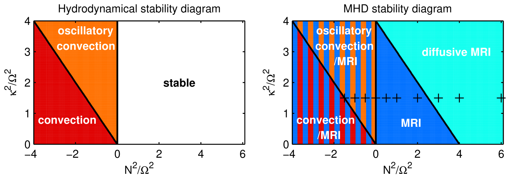
Figure 1: Stability diagram as a function of the square of the Brunt-Väisälä frequency $N^{2}$ (characterizing the influence of buoyancy) and the square of the epicyclic frequency $\kappa^{2}$ (characterizing the effect of rotation and shear). The left panel applies to hydrodynamic flows and shows the regions unstable against classical convection (red) and oscillatory convection enabled by thermal diffusion (orange). The right panel applies to MHD flows and shows the region unstable against the MRI (blue) including the also convectively unstable regions (red and orange regions with blue stripes) and the diffusive MRI enabled by thermal diffusion (turquoise). The plus signs give the parameters of our simulations (those for $N^{2}/\Omega^{2}=8$ and 10 are not shown).

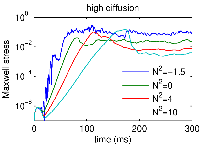
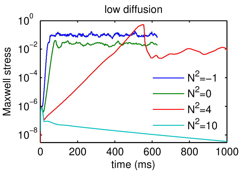
Figure 2: Time evolution of the box averaged Maxwell stress for simulations with different stratifications, i.e. different values of $N^{2}/\Omega^{2}$, for high ($P_{e}=100$; left panel) and low ($P_{e}=1000$; right panel) thermal diffusion. Note that the time interval is different in the two panels.

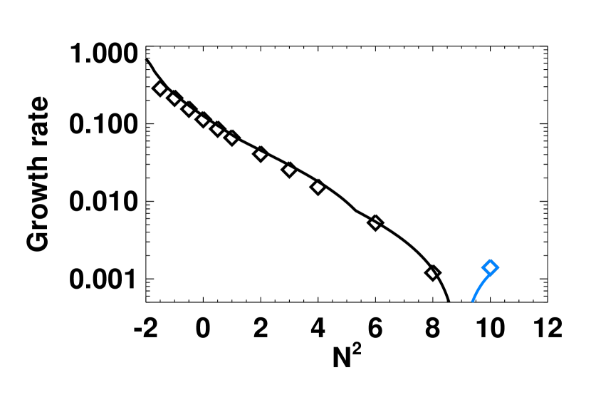
Figure 3: Comparison of the growth rates as a function of the strength of buoyancy as measured by $N^{2}/\Omega^{2}$ obtained from our numerical simulations (diamonds) and our linear analysis (solid lines; see Appendix A and B) for high ($P_{e}=100$; left panel) and low ($P_{e}=1000$, right panel) thermal diffusion. The dotted line gives the prediction of the linear growth rate in a hydrodynamic flow (Appendix B). Blue colour is used when the growth rate is negative, i.e. when it gives the damping rate. We normalized both the growth rate $\sigma$ and the Brunt-Väisäla frequency $N$ by the angular frequency $\Omega$.

Let us start this section by discussing stability conditions in the presence of buoyancy and differential rotation both in hydrodynamic and MHD flows. We restrict this discussion to the special case considered in this paper: a local box in the equatorial plane of the PNS, where the angular frequency, entropy and composition depend only on radius. We further restrict the discussion to axisymmetric perturbations and to flows which are stable against the hydrodynamic shear instability, i.e. complying with the Rayleigh stability criterion $\kappa^{2}>0$, where $\kappa$ is the epicyclic frequency defined by

$$\kappa^{2}\equiv\frac{1}{r^{3}}\frac{{\rm d}(r^{4}\Omega^{2})}{{\rm d}r}.$$ (28)

We first consider stability conditions in the absence of any diffusive process. If

$$\kappa^{2}+N^{2}<0$$ (29)

the flow is convectively unstable because the Solberg-Høiland stability criteria is violated (red region in Fig. 1). In the presence of magnetic field the condition reads

$$\kappa^{2}+N^{2}<4\Omega^{2}.$$ (30)

This criterion is less restrictive than the hydrodynamic one due to the appearance of the MRI for $0<\kappa^{2}+N^{2}<4\Omega^{2}$ (dark blue region, and red and orange regions with blue stripes in the right panel of Fig. 1). The classical MRI (i.e. in the absence of buoyancy effect) is obtained for $N^{2}=0$ and $0<\kappa^{2}<4\Omega^{2}$.

When thermal diffusion is present (but no resistivity and viscosity), the instability region is more extended for two reasons. First, thermal diffusion alleviates the stabilising effect of buoyancy on the MRI (Acheson, 1978; Menou et al., 2004; Masada et al., 2007). As a consequence the MRI instability criterion becomes $0<\kappa^{2}<4\Omega^{2}$, i.e. the MRI unstable region now comprises a region that is stable according to equation (30) (turquoise region in the right panel of Fig. 1).

Another consequence of thermal diffusion is the appearance of a new hydrodynamic instability (Klahr & Hubbard, 2014; Lyra, 2014), which we refer to as oscillatory convection. It occurs for $N^{2}<0$ in a parameter regime that is stable according to equation (29) (orange region in Fig. 1). Oscillatory convection can be considered to be an analog of semi-convection (in which thermal diffusion causes the flow to be unstable in the presence of an otherwise stabilising composition gradient), rotation assuming the role of the stabilising composition gradient in the case of semi-convection.

The parameter regime explored with our simulations is shown with plus signs in Fig. 1. We varied the Brunt-Väisälä frequency in the range $-1.5<N^{2}/\Omega^{2}<10$ and fixed the epicyclic frequency to a value $\kappa^{2}/\Omega^{2}=1.5$. Hence, we explored three regimes: non-diffusive MRI for $0<N^{2}<2.5$, diffusive MRI (i.e. allowed by thermal diffusion) for $N^{2}>2.5$, and a mixed regime where MRI and oscillatory convection can co-exist for $-1.5<N^{2}<0$. Note that in none of our simulations the flow is unstable to axisymmetric classical (non-oscillatory) convection.

Figure 2 shows the time evolution of the Maxwell stress averaged over the computational box. After a linear phase of exponential growth, the Maxwell stress saturates in the non-linear phase. In this section we analyse only the linear phase and postpone the analysis of the non-linear phase to next section. All but two simulations show a non-oscillatory growth, which is due to the MRI modified by buoyancy. For low thermal diffusion ($P_{e}=1000$; right panel), the growth rate varies by orders of magnitudes and becomes extremely small for large positive values of $N^{2}$, up to the point that no growth occurs at all for $N^{2}/\Omega^{2}=10$. By contrast, for high thermal diffusion ($P_{e}=100$; left panel), the effect of buoyancy on the growth of the MRI is much less pronounced. The MRI can still grow in a short time even for large values of $N^{2}$. A good agreement is obtained between the growth rates obtained from our numerical simulations and the predictions from the linear analysis presented in Appendix A (Fig. 3).

Our results are in qualitative agreement with those of Masada et al. (2007), who showed that the MRI can grow unimpeded by stable buoyancy if the thermal diffusivity is sufficiently large compared to the viscosity, i.e. if $\chi>\nu N/\Omega$. This condition is indeed verified for high thermal diffusion ($P_{e}=100$ and $\chi/\nu=10$), in which case the growth of the MRI is only mildly affected by buoyancy. By contrast, the growth of the MRI is drastically suppressed in the case of low thermal diffusion and large $N^{2}/\Omega^{2}$ ($P_{e}=1000$ and $\chi=\nu$), i.e. if the above condition is not fulfilled. Note that, even for a high diffusivity, the MRI growth rates are significantly smaller than those of the ideal MRI ($\sigma/\Omega=q/2=0.625$). This stands in contrast to the situation considered by Masada et al. (2007) and is due to the fact that we considered a magnetic field strength that lies in the viscous regime, where the MRI growth is significantly slowed down by neutrino viscosity (Guilet et al., 2015).

One of our simulations with unstable buoyancy and high thermal diffusion ($N^{2}/\Omega^{2}=-1.5$ and $P_{e}=100$) showed an oscillatory exponential growth due to the oscillatory convection discussed above. The transition of the fastest growing mode from MRI to oscillatory convection is clearly seen in Fig. 3 for high thermal diffusion, where it happens at $N^{2}\ \sim-\Omega^{2}$ in agreement with the linear prediction. In the regime of oscillatory convection, the growth rate predicted by the hydrodynamic linear analysis presented in Appendix B matches that of the MHD linear analysis and the simulations, clearly demonstrating the hydrodynamic nature of the instability.

4 Non-linear phase

When the exponentially growing axisymmetric (i.e. y-independent) MRI channel modes reach non-linear amplitudes, non-axisymmetric secondary (or ”parasitic”) instabilities start to grow upon the primary modes (Goodman & Xu, 1994; Pessah & Goodman, 2009; Latter et al., 2009; Obergaulinger et al., 2009; Pessah, 2010). This leads to the disruption of the channel modes, thereby ending the exponential growth phase. From that point on the dynamics consists, in most cases, of 3D statistically steady MHD turbulence. A somewhat different dynamics takes place, however, in the case of low thermal diffusion ($P_{e}=1000$) and a sufficiently stabilising buoyancy $N^{2}/\Omega^{2}\gtrsim 3$. In that case, we observed the recurrent emergence of exponentially growing channel flows and their subsequent disruption by parasitic instabilities. The resulting dynamics is fundamentally non-steady due to this quasi-periodic emergence of the large scale channel flows. For high thermal diffusion we did not observe recurrent channel flows, but nonetheless noticed the development of long-lived coherent flow structures in the regime where the flow is stable against buoyancy. Therefore, we split the following discussion of the properties of the non-linear phase into two subsections. The first one we devote to the coherent flows (either recurrent or statistically steady), while we discuss in the second subsection the time and volume averaged properties of the flow during the non-linear phase.

4.1 Coherent flows

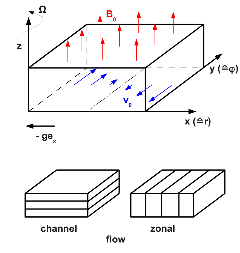
Figure 4: Schematic representation of the shearing box geometry (upper panel) and of the geometry of the coherent flows (lower panels): channel flows (left-hand lower panel) and zonal flows (right-hand lower panel).

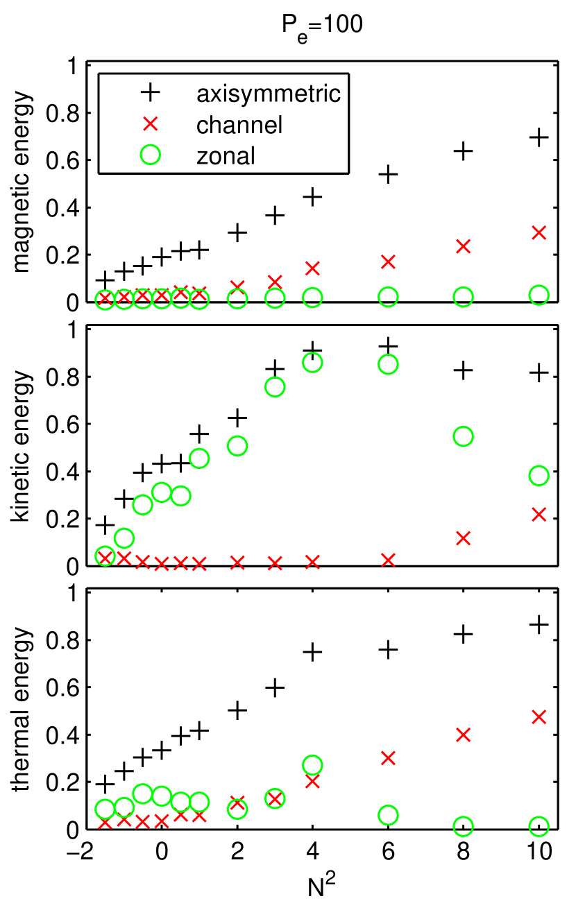
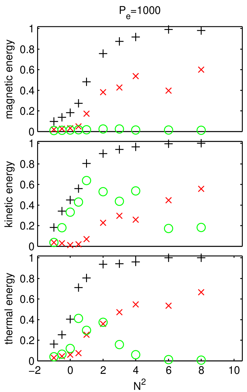
Figure 5: Fraction of magnetic (top row), kinetic (middle row), and thermal (bottom row) energy densities contained in axisymmetric structures (black $+$ symbols), channel flows (red $\times$ symbols), and zonal flows (green circles) for simulations performed with high thermal diffusion ($P_{e}=100$; left column) and low thermal diffusion ($P_{e}=1000$; right column).

In the stable buoyancy regime ($N^{2}>0$), we observe the appearance of either long lived (for $P_{e}=100$) or recurrent (for $P_{e}=1000$) coherent structures in the non-linear state of the MRI. Two different types of such coherent structures can be distinguished (Figure 4): channel flows with a vertically varying but horizontally uniform structure (i.e. flow quantities only depend on coordinate $z$), and zonal flows with a radially varying but azimuthally and vertically uniform structure (i.e. flow quantities only depend on coordinate $x$).

Channel flows are related to the most unstable linear modes of the MRI in case of a vertical background magnetic field. These modes, which have a purely vertical wavenumber, i.e. $\bm{k}=(0,0,k_{z})$, are known to be non-linear growing solutions of the MHD equations (Goodman & Xu, 1994). They are unstable to parasitic instabilities of Kelvin-Helmholtz or resistive tearing mode type (Goodman & Xu, 1994; Latter et al., 2009; Pessah & Goodman, 2009; Pessah, 2010; Obergaulinger et al., 2009), the development of which can stop the growth of the channel mode and trigger turbulence. The typical structure of MRI channel modes consists of a sinusoidal profile that holds for the horizontal (i.e. x and y) components of both velocity and magnetic field , and in the presence of buoyancy for the buoyancy variable $\theta$ (equation 6), too. As can be deduced from Eqs. (46)–(48), in MRI channel modes the radial (x) and azimuthal (y) velocity components are typically in phase , while the radial and azimuthal magnetic field components are typically in anti-phase with each other . They are shifted also by a quarter of a wavelength with respect to the horizontal (x,y) velocity components, whereas the buoyancy variable $\theta$ is in phase with these components (equation 49).

Zonal flows have been observed in shearing box simulations of MRI turbulent stratified accretion discs (Johansen et al., 2009; Simon et al., 2012; Simon & Armitage, 2014). They mostly possess a radially varying azimuthal velocity, which is associated with a radial variation of the pressure. In the presence of a mean vertical magnetic field, a radial variation of the vertical magnetic field has been reported recently too (Bai, 2014; Bai & Stone, 2014).

Figure 5 illustrates the occurrence of the different types of coherent flows as a function of the Brunt-Väisälä frequency by showing the fractions of kinetic, magnetic, and thermal energy densities contained in axisymmetric structures, channel flows, and zonal flows, respectively. To obtain the energy densities contained in axisymmetric structures we first averaged the magnetic field, velocity, and buoyancy variable in azimuthal (y) direction. Then we used these averages to compute the respective energy densities averaging over the box and over time. Instead, we first averaged the flow variables horizontally (i.e. both in azimuthal (y) and radial (x) direction) to compute the energy densities contained in channel flows. Finally, for the zonal flows, we first averaged the flow variables in vertical (z) and azimuthal (y) direction.

Figure 5 demonstrates that the flow becomes more axisymmetric for increasing $N^{2}$, i.e. for flows that are more stable to buoyancy. This holds for the magnetic, kinetic, and thermal energies at both low and high thermal diffusion but is more pronounced at low thermal diffusion, in qualitative agreement with the idea that high thermal diffusion somewhat alleviates the influence of a stabilising buoyancy. The prominence of channel flows also increases monotonically with $N^{2}$ for all three energies and at both thermal diffusivities. This behaviour is again more pronounced at low thermal diffusion, where the channel flows contain up to about $50\%$ of the energy. As already mentioned the channel flows have a different time behaviour at $P_{e}=100$ and $P_{e}=1000$. At high thermal diffusion they are approximately steady (see Section 4.1.1), while at low thermal diffusion they show recurrent phases of exponential growth and disruption (see Section 4.1.3).

Zonal flows stick out most clearly regarding the kinetic energy (remarkably, their fraction can reach up to $90\%$), while they amount to a lesser fraction of the thermal energy, and an almost negligible fraction of the magnetic energy. Their dependence on $N^{2}$ is more complex than that of the channel flows. While their importance first increases with $N^{2}$ (up to $N^{2}=4-6$ at $P_{e}=100$, and $N^{2}=2$ at $P_{e}=1000$), it starts to decrease at still higher $N^{2}$. As for the channel flows, zonal flows have a different time behaviour at high and low diffusion. They are approximately steady and long-lived at $P_{e}=100$ (Section 4.1.2), but recurrent at $P_{e}=1000$ (Section 4.1.3).

4.1.1 Quasi-stationary channel flows

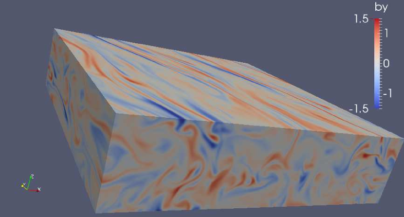
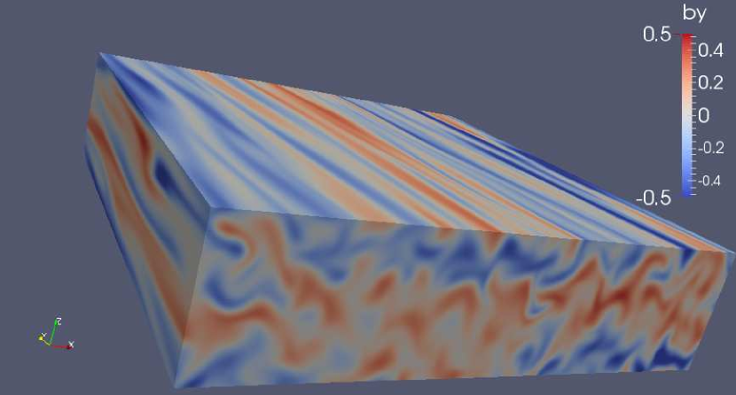
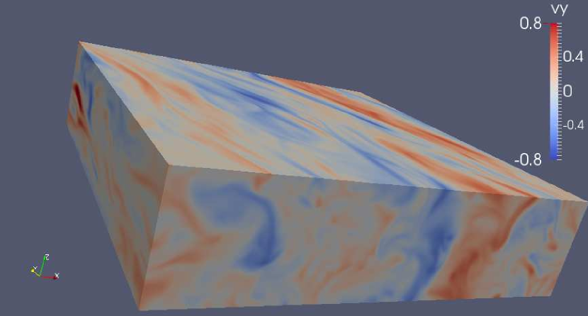
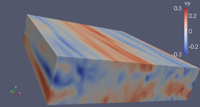
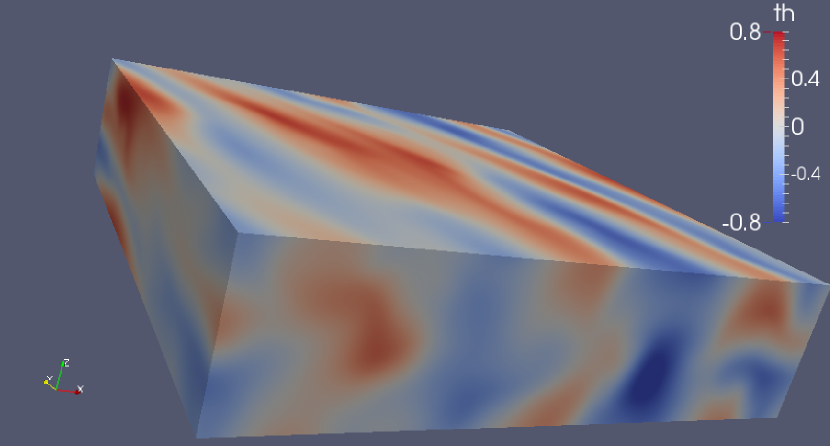
Figure 6: Three-dimensional snapshots at time $t=553\,{\rm ms}$ of two simulations with $P_{e}=100$ for a buoyantly unstable flow with $N^{2}/\Omega^{2}=-1$ (left column) and buoyantly stable flow with $N^{2}/\Omega^{2}=10$ (right column). The three rows show the azimuthal magnetic field (top), azimuthal velocity (middle), and buoyancy variable $\theta$ (bottom). Note that we adjusted the colour scales to the level of turbulence, i.e. they are different for the two columns.

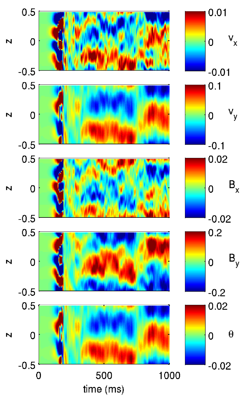
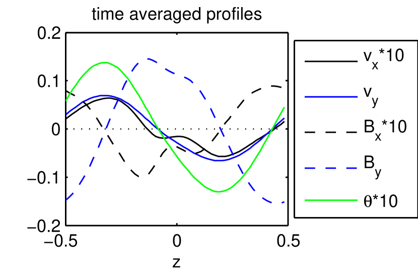
Figure 7: Quasi-stationary channel flow for $N^{2}/\Omega^{2}=10$ and high thermal diffusion $P_{e}=100$. The upper five panels show space time diagrams (from top to bottom) of the horizontally averaged radial velocity, azimuthal velocity, radial magnetic field, azimuthal magnetic field, and buoyancy variable $\theta$. The bottom panel gives the vertical profiles of these quantities averaged over the time interval $400\,{\rm ms}\leq t\leq 700\,{\rm ms}$.

Figure 6 shows snapshots of the azimuthal magnetic field, the azimuthal velocity, and the buoyancy variable for two simulations at high thermal diffusion for a flow unstable ($N^{2}/\Omega^{2}=-1$; left column) and stable ($N^{2}/\Omega^{2}=10$; right column) to buoyancy. In the latter case, the flow is much more axisymmetric, and we observe a channel flow structure superposed to a disordered flow.

The channel flow structure and time-evolution can be made more apparent by calculating horizontal averages of the flow variables. We show space-time diagrams of these averages in Fig. 7 for the simulation with $N^{2}/\Omega^{2}=10$ and $P_{e}=100$. A first transient phase of strong channel flow occurs between $t\sim 100\,{\rm ms}$ and $200\,{\rm ms}$ corresponding to the MRI channels of the exponential growth phase described in Section 3. After the disruption of these channels by parasitic instabilities and the onset of turbulence, one observes no clear channel flow until $t\sim 300\,{\rm ms}$. At that moment, another channel flow appears whose amplitude and phase is remarkably steady until the end of the simulation, except for a phase shift that takes place around $t\sim 750\,{\rm ms}$. To our knowledge, this is the first time that such a stationary channel flow has been seen to appear in MRI turbulence (only recurrent channel flows were sometimes observed as will be discussed in Section 4.1.3).

Let us now compare the structure of this stationary channel flow to that of growing linear MRI modes. From the space-time diagrams (Fig. 7) it is already clear that the wavelength of the stationary flow (one wavelength fits into the box) is longer than that of the exponentially growing mode (a mixture of modes with $n=2$ and $n=3$ wavelengths fit into the box), the latter one corresponding to the linear prediction . Obviously, the quasi-stationary channel flow does not correspond to the most unstable MRI mode. The time-averaged profiles (Fig. 7; bottom panel) show nonetheless interesting qualitative similarities with linear MRI modes. The profiles resemble quite closely that of a sinusoidal function whose wavelength is equal to the vertical size of the box, except for the profiles of the radial velocity and the magnetic field which both show some indication of smaller scale structure on top of the dominant $n=1$ sinusoid. Interestingly, the radial velocity, azimuthal velocity, and buoyancy variable are in phase, while the radial and azimuthal magnetic fields are in anti-phase and shifted by a quarter of a wavelength with respect to the velocity profiles. This result is in accordance with the structure of a linear MRI channel mode, and it suggests a link between the stationary channel flow and linear MRI modes.

In view of the qualitative similarity but quantitative difference between the stationary channel flow and the linear MRI modes, we interpret the stationary channel flow as an MRI channel mode significantly modified by the concurrent turbulence, which presumably brings it to marginal stability. Further studies of the physics of the stationary channel flow and its interaction with turbulence may shed light on the mechanism determining the level of MHD turbulence. Using enlarged diffusion coefficients to roughly describe the impact of turbulence on the channel flow may provide the basis for modelling MRI saturation and could allow for a deeper interpretation of the numerical simulations. One could, for example, speculate that the level of turbulence adjusts so as to bring the largest scale MRI mode to marginal stability (Ogilvie & Livio, 2001; Guilet & Ogilvie, 2012, 2013).

4.1.2 Quasi-stationary zonal flows

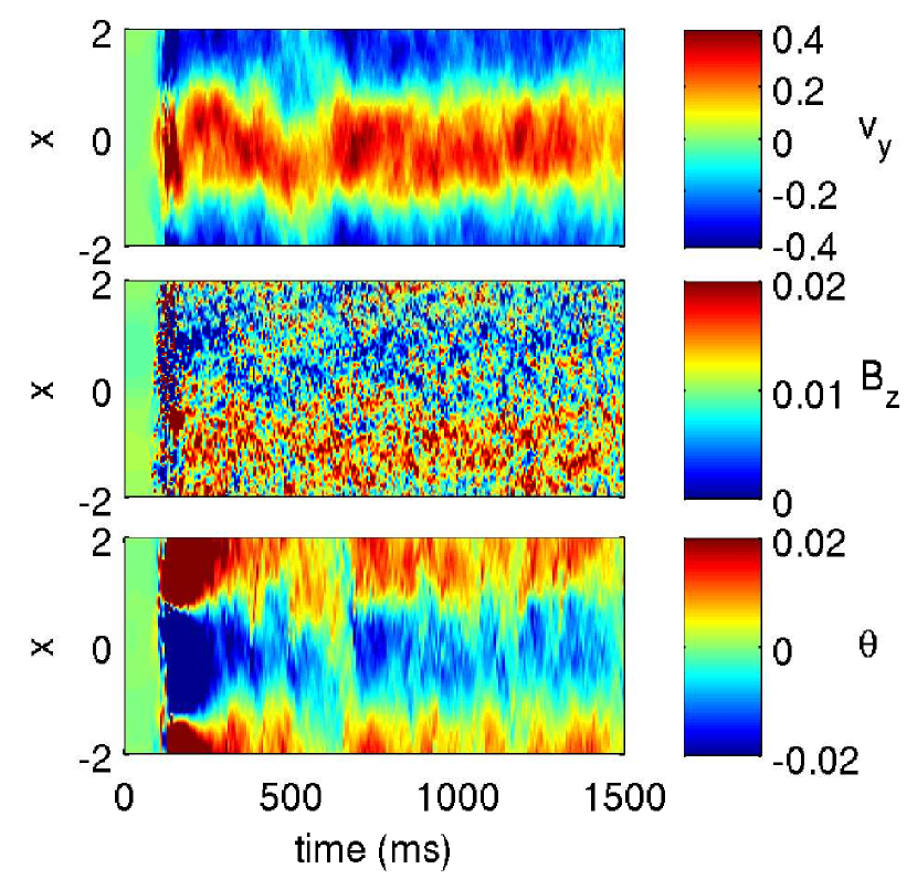
Figure 8: Space-time diagrams for a zonal flow with $N^{2}/\Omega^{2}=4$ and $P_{e}=100$. The three panels show the azimuthal velocity (top), the vertical magnetic field (middle), and the buoyancy variable $\theta$ (bottom). These quantities are averaged in azimuthal (y) and vertical (z) direction, and plotted as a function of time and radius (x).

Zonal flows can conveniently be visualised with a space-time diagram showing the radial profile of azimuthally and vertically averaged quantities. Fig. 8 shows such a diagram for a simulation with $N^{2}/\Omega^{2}=4$ and $P_{e}=100$, where a very stable quasi-stationary zonal flow is clearly visible. It shows that azimuthal velocity has by far the largest amplitude amounting to $\sim 90\%$ of the kinetic energy, but a modulation with a wavelength equal to the radial size of the box is also recognisable in the vertical magnetic field and the buoyancy variable. The modulation of the vertical magnetic field is shifted by a quarter of a wavelength with respect to that of azimuthal velocity (i.e. the maximum of the magnetic field corresponds to a zero of the velocity), in agreement with the results of Bai & Stone (2014). We note that the magnetic field zonal modulation represents a negligible fraction of the total magnetic energy (see Fig. 5), but it amounts to a significant fraction of the mean vertical magnetic field. Thus, it may play a significant role in the flow dynamics.

The zonal flow shown in Fig. 8 is representative of flows for Brunt-Väisälä frequencies $3\lesssim N^{2}/\Omega^{2}\lesssim 6$. In this parameter regime, the zonal flow dominates the kinetic energy, and it is very stable and quasi-steady. At lower and higher values of $N^{2}$, zonal flows tend to be more noisy and less stable in that their phase changes somewhat chaotically with time on timescales of ten or a few tens of orbits.

4.1.3 Recurrent channel and zonal flows

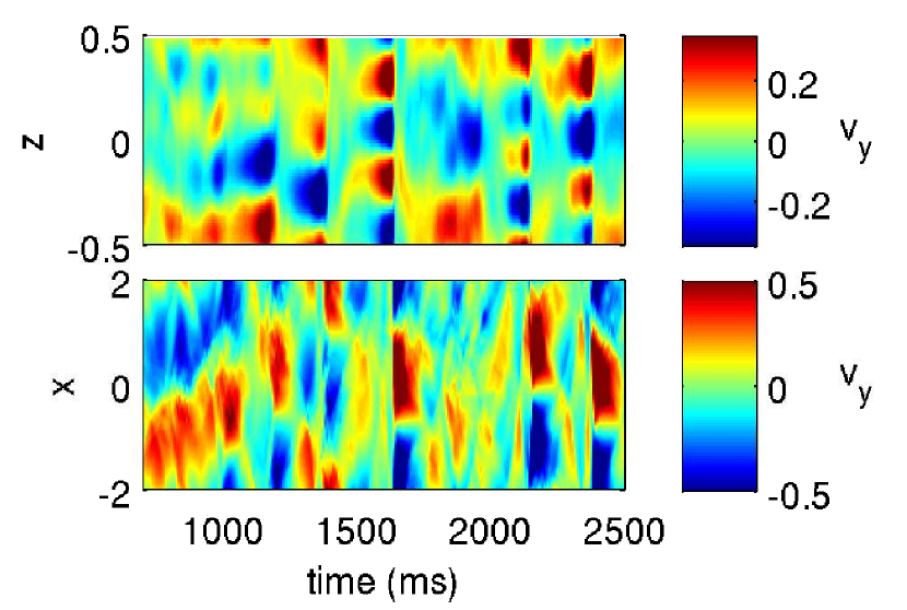
Figure 9: Space-time diagrams of the azimuthal velocity for $N^{2}/\Omega^{2}=4$ and $P_{e}=1000$. The upper panel shows horizontally averaged vertical profiles, where recurrent channel flows are clearly visible. The lower panel shows vertically and azimuthally averaged radial profiles, where transient zonal flows can be recognised just after the disruption of the channel flows.

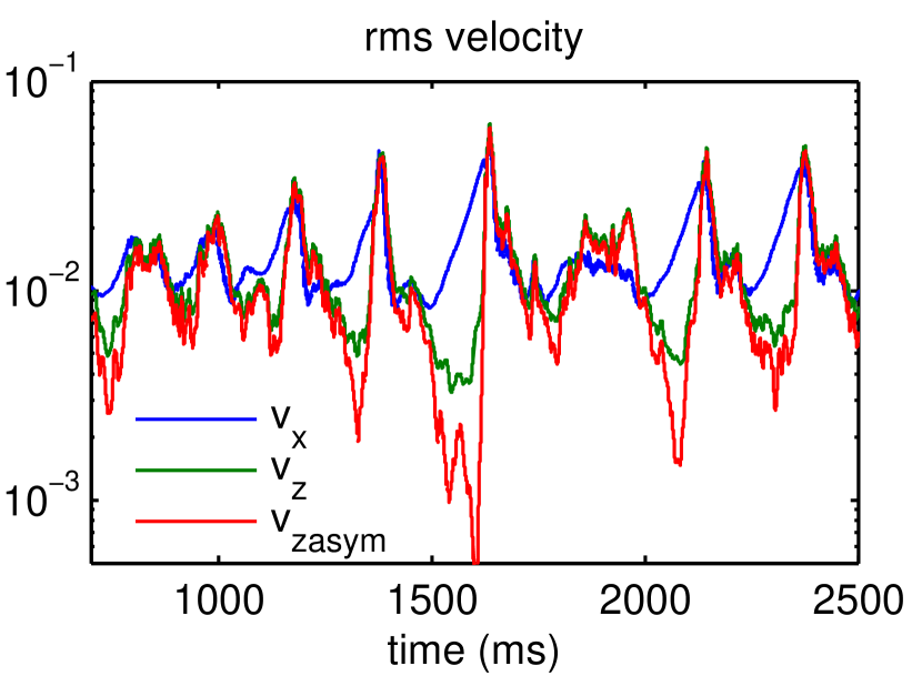
Figure 10: Time evolution of various box averaged quantities showing the recurrent growth of channel and zonal flows for a simulation with $N^{2}/\Omega^{2}=4$ and $P_{e}=1000$. Left panel: time evolution of the kinetic energy (blue), the kinetic energy of the channel flow (green), and the kinetic energy of the zonal flow (red). Right panel: time evolution of the rms averages of the radial velocity (blue), vertical velocity (green), and the non-axisymmetric component of the vertical velocity (red).

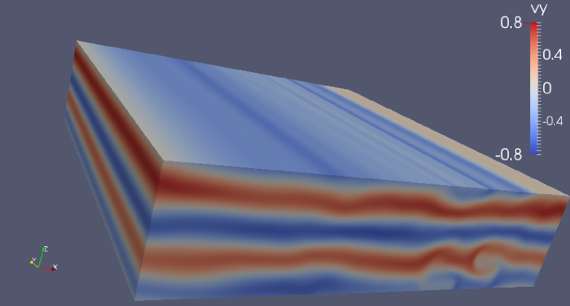
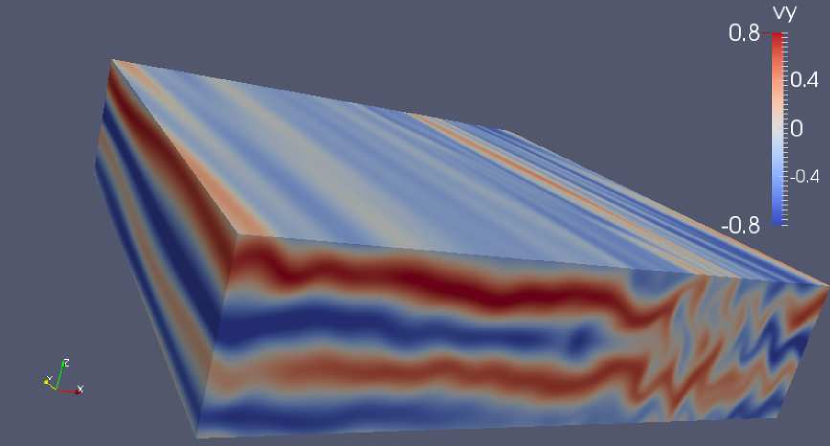
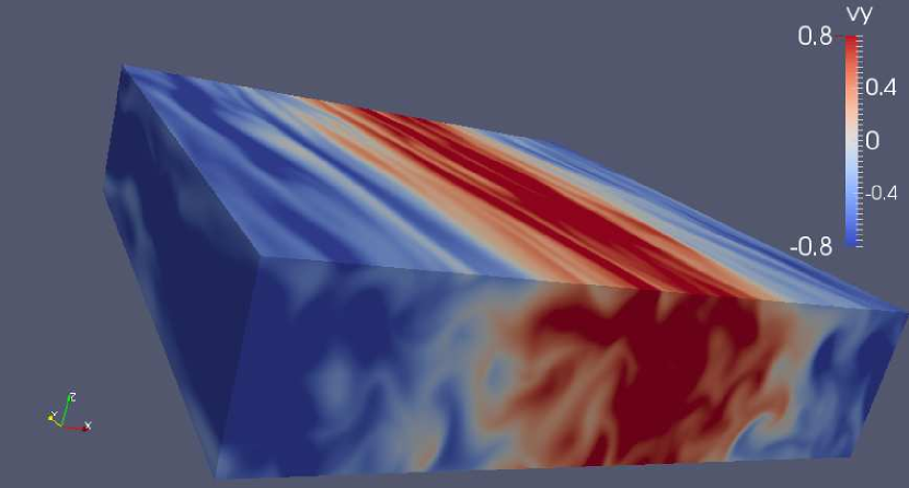
Figure 11: Three snapshots of the azimuthal velocity illustrating the time evolution of recurrent channel and zonal flows for a simulation with $N^{2}/\Omega^{2}=4$ and $P_{e}=1000$: exponential growth of a channel mode (upper panel), its disruption (middle panel), and the formation of a zonal flow after the disruption of the channel mode (bottom panel). The snapshots are separated in time by two orbital periods, and they correspond (from top to bottom) to times $t=1615$, $1627$, and $1640\,{\rm ms}$, respectively.

At low thermal diffusion and in the stable buoyancy regime, channel and zonal flows are present too. However, contrary to the high diffusion case, they are not quasi-stationary. This is illustrated in Fig. 9 with space-time diagrams of the azimuthal velocity for $N^{2}/\Omega^{2}=4$ and $P_{e}=1000$. The vertical profile of the horizontally averaged azimuthal velocity, $\langle v_{y}\rangle_{x,y}(z)$ (top panel), shows recurrent phases of channel mode growth and sudden disruption. The radial profile of the vertically and azimuthally averaged azimuthal velocity, $\langle v_{y}\rangle_{y,z}(x)$ (middle panel) shows that the disruption of the channel flow is accompanied by the formation of a strong zonal flow. This zonal flow then decays and another phase of channel flow growth begins. These successive phases of channel flow growth, disruption, and zonal flow formation can also be seen in the left panel of Fig. 10, which demonstrates that the formation of the zonal flow exactly coincides with the disruption of the channel flow. The right panel shows that during the phase of exponential growth of the channel flow, the radial velocity (as well as the even higher azimuthal velocity (not shown)) is much larger than the vertical velocity, consistent with a channel mode dominating the flow. Furthermore, the flow is mostly axisymmetric, as can be deduced from the fact that the non-axisymmetric part of the vertical velocity is significantly smaller than the total vertical velocity. The growth of non-axisymmetric parasitic instabilities disrupting the channel mode is visible in the sudden rise of the vertical velocity, and in particular of its non-axisymmetric part. The disruption of the channel flow is then followed by a phase of decaying non-axisymmetric turbulence, during which the radial velocity, the vertical velocity and the non-axisymmetric part of the vertical velocity have similar magnitudes.

Recurrent channel flow growth and disruption by parasitic instabilities has already been observed in numerical simulations of the MRI in the absence of buoyancy (e.g. Lesur & Longaretti, 2007). Lesur & Longaretti (2007) argued that this behaviour is characteristic of the MRI growing close to its threshold of marginal stability, be it because the magnetic field is very strong, or the resistivity and viscosity are very high. This interpretation is consistent with the results of our simulations, where the MRI is brought close to marginal stability by the effect of buoyancy.

Figure 11 illustrates the phases of channel flow (top panel), its disruption (middle panel), and the formation of a zonal flow (bottom panel). The upper panel shows an almost pure horizontally uniform channel flow, with only slight perturbations to the right hand side of the box. Two orbits later, these perturbations have grown due to parasitic instabilities, and the channel flow is being disrupted first on the right hand side of the box, and afterwards in the rest of the box, such that two orbits later the channel flow has completely disappeared and a zonal flow has formed. We attribute the formation of the zonal flow to the non-uniformity of the channel flow disruption over the radial extent of the box. Indeed, as the disruption of the channel flow happens first on the right hand side of the box ($1\lesssim x\lesssim 2$), the Maxwell and Reynolds stresses are first quenched in that part of the box, while they remain high in the rest of the box. Before the disruption extends to the rest of the box, the angular momentum flux is therefore non-uniform and the redistribution of angular momentum creates the zonal flow. To our knowledge, such episodic zonal flow formation due to the disruption of a channel flow has never been reported before. Since the mechanism we propose does not seem directly related to the impact of buoyancy (whose role is mostly to bring the MRI close to marginal stability), we suggest that it may also take place in the classical MRI without buoyancy.

The dynamics described in this section for $N^{2}/\Omega^{2}=4$ is characteristic of simulations with $N^{2}/\Omega^{2}\gtrsim 3$. In this regime, as $N^{2}$ increases the typical timescale between phases of channel flow growth becomes longer. This can be interpreted by the smaller growth rate of the linear channel modes (see Fig. 3), which therefore take a longer time to grow again after their disruption. Note that for $N^{2}/\Omega^{2}\simeq 1-2$ and $P_{e}=1000$, the zonal and channel flows are more similar to the case of high thermal diffusion: quasi-stationary, though somewhat more variable than those shown in Sections 4.1.1 and 4.1.2.

4.2 Time-averaged properties

To characterize the properties of the non-linear state and its dependence on $N^{2}$, we performed time and box averages of the magnetic, kinetic and thermal energies, the energy injection rates, and the rms values of the three spatial components of velocity and magnetic field. For each simulation, we adapted the time at which the averaging is started to avoid the initial transient dynamics (the first exponential channel growth phase, sometimes followed by a transient zonal flow). Because of the slower growth in the stable buoyancy regime, some simulations had to be run for a longer time period in order to obtain a meaningful average over the non-linear phase (see Table 1; note that $6.28\,{\rm ms}$ correspond to one orbit).

Table 1: Time averaging intervals

$P_{e}$	$N^{2}/\Omega^{2}$	interval [msec]
100	$\leq 4$	[1 200, 1 628]
	6	[1 400,  1000]
	8	[ 1000,  2000]
	10	[1 400,  1000]
1000	$\leq 0.5$	[1 200, 1 628]
	1	[1 300,  1600]
	2	[ 1000,  3000]
	3	[ 1000,  3000]
	4	[ 1000,  3000]
	6	[ 2000,  6000]
	8	[ 3000, 10000]

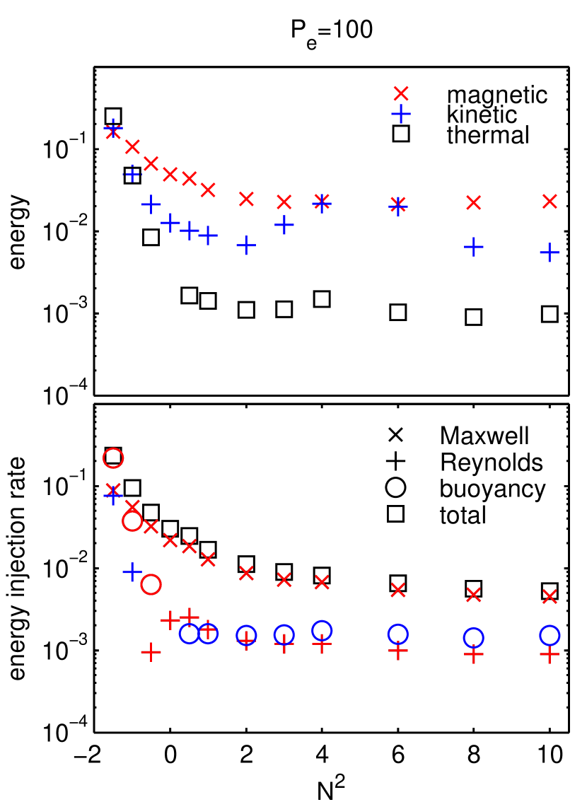
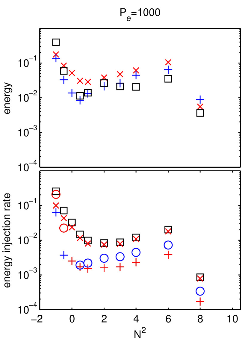
Figure 12: Time and volume averages of the turbulent energy densities and energy density injection rates as a function of the Brunt-Väisälä frequency. Panels in the left and right column correspond to high ($P_{e}=100$) and low ($P_{e}=1000$) thermal diffusion, respectively. They show the magnitude of magnetic (red $\times$), kinetic (blue $+$), and thermal (black squares) energies in the top panels, and energy injection rates due to Maxwell stress ($\times$ symbols), Reynolds stress ($+$ signs), buoyancy force work (circles), and sum of the three (squares) in the bottom panels. Positive injection rates are shown in red colour, while negative ones (i.e. energy is removed from turbulent motions) are shown in blue.

Figure 12 illustrates how the magnetic, kinetic, and thermal energies, and the energy injection rates depend on the Brunt-Väisälä frequency. For high thermal diffusion, magnetic energy and Maxwell stress decrease monotonically with $N^{2}$, as one may intuitively expect. Importantly, the dependence gets much weaker as $N^{2}$ increases, to the extent that the magnetic energy is practically independent of $N^{2}$ for $N^{2}/\Omega^{2}\geqslant 3$, while the Maxwell stress very slowly declines in this regime. As a result, the magnetic energy is more affected by an unstable buoyancy, than by a stable one. It increases by a factor of $3.3$ between $N^{2}=0$ and $N^{2}/\Omega^{2}=-1.5$, but it decreases only by a factor $2.2$ between $N^{2}=0$ and $N^{2}/\Omega^{2}=10$. In the stable buoyancy regime ($N^{2}>0$), the thermal energy and the corresponding injection rate are almost independent of $N^{2}$, and both are much smaller than the corresponding magnetic quantities. By contrast, in the unstable buoyancy regime, they increase rapidly in magnitude as $N^{2}$, up to the point where the thermal energy and the corresponding injection rate are the dominant contributions at $N^{2}/\Omega^{2}=-1.5$, suggesting that turbulence is driven then more by buoyancy than by the shear. Note that the increased turbulence strength in the unstable buoyancy regime is similar to that observed in the context of accretion discs by Hirose et al. (2014) and Hirose (2015). The geometry is nonetheless different: in accretion discs the buoyancy force is mostly vertical, while in our setup it is radial.

At low thermal diffusion, we found qualitatively similar trends for $N^{2}/\Omega^{2}\lesssim 1$, but with a somewhat steeper dependence on $N^{2}$, a result which agrees with the idea that a lower thermal diffusion allows buoyancy to act more effectively. The behaviour for $2-3\lesssim N^{2}/\Omega^{2}\lesssim 6$ is more surprising. All energies and energy injection rates increase in magnitude with $N^{2}$, in spite of the fact that, as in the high diffusion case, buoyancy is actually removing energy from the flow (because the buoyancy injection rate is negative). This behaviour is found in the parameter regime showing strong recurrent channel flows, where the energy is predominantly contained in axisymmetric structures (see Section 4.1). The increase in energy and energy injection rate is due to the fact that, at higher $N^{2}$, recurrent channel flows reach larger amplitudes before they are disrupted by parasitic instabilities. The cause of the increase of the channel flow amplitude at termination is unclear, but may be linked to the so far unknown impact of buoyancy on parasitic instabilities. In this respect it is interesting to note that, at high thermal diffusion, the amplitude at which the first phase of channel mode growth is terminated increases with $N^{2}$ (as can be seen in Fig. 2). This may be linked to the increasing energy observed in the non-linear phase for low thermal diffusion. It also highlights the fact that the amplitude at which channel mode growth is terminated is not necessarily correlated with the strength of MRI turbulence (which decreases with $N^{2}$ for high thermal diffusion).

Figures 13 and 14 show the dependence of the ratio of different flow quantities on $N^{2}$: Reynolds stress to Maxwell stress (top left), kinetic energy to magnetic energy (top right), radial to azimuthal velocity amplitudes (bottom left), and radial to azimuthal magnetic field amplitudes (bottom right). An advantage of studying such ratios is that they allow for a comparison of the flow properties of the non-linear phase to that of linear channel flows (Pessah et al., 2006). Indeed, while the amplitude of a quantity (say the Reynolds stress) due to a channel mode is unknown if one does not know a priori the mode amplitude, the ratio of two quantities (e.g. Reynolds stress to Maxwell stress) is well defined for a channel mode independently of its amplitude (see Appendix A). Figure 13 shows that, at low thermal diffusion, all these ratios vary significantly with $N^{2}$ and are in general agreement with the prediction from the linear modes. This agreement is not surprising in the regime of stable buoyancy where channel modes contribute a significant fraction of the energy, but it is surprising in the regime of unstable buoyancy where the fraction of energy contained in channel modes is insignificant. The (at least qualitative) agreement in the latter regime therefore suggests that linear dynamics leaves an imprint on the properties of turbulence even when channel modes do not dominate the flow.

Interestingly, in the regime of unstable buoyancy ($N^{2}/\Omega^{2}=-1$ and $-0.5$) the Reynolds stress changes sign and becomes negative, while it is always positive (corresponding to an outward transport of angular momentum) for the MRI in the absence of buoyancy. At $P_{e}=1000$, this behaviour is reproduced amazingly well by the linear analysis. When the Reynolds stress becomes negative, the Coriolis force is not anymore a driver of the radial motion in the channel mode contrary to the classical MRI. Then the buoyancy force drives the radial motion instead. The magnetic field nevertheless still plays a crucial role in the instability mechanism by reducing the stabilising effect of the Coriolis force, because no non-oscillatory growth is possible in this regime in the absence of a magnetic field (see Section 3). Hence, we interpret the instability in the unstable buoyancy regime as a mixed magneto-rotational buoyant instability, and the increasing ratio of kinetic to magnetic energy by the increasing role played by the buoyancy force compared to the magnetic one.

Another interesting trend visible in Fig. 13 concerns both the ratio of azimuthal to radial velocity and the ratio of azimuthal to radial magnetic field. These ratios increase tremendously with $N^{2}$, reaching a value of $100$ for the former one. This may qualitatively be interpreted by the fact that for increasing $N^{2}$, the buoyancy force prevents more and more efficiently radial motions. In the regime of stable buoyancy magnetic and kinetic energy are therefore dominated by the azimuthal component of the magnetic field and the velocity, respectively. The vertical components of both quantities (not shown) are of the same order of magnitude as their radial components.

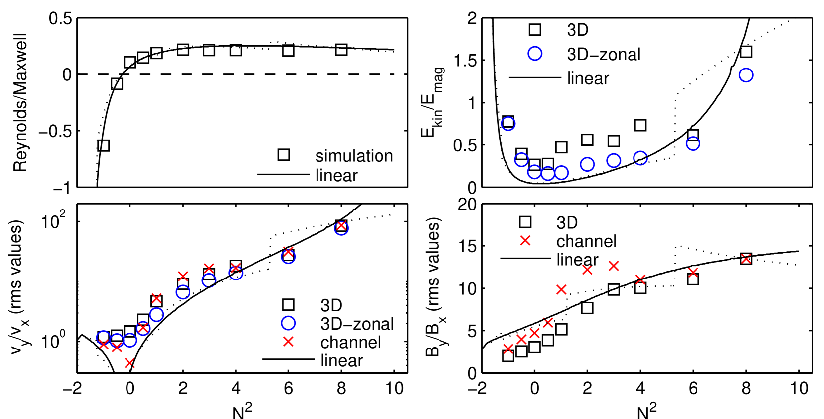
Figure 13: Ratios of different time and volume averaged diagnostics as a function of $N^{2}/\Omega^{2}$ for low thermal diffusion ($Pe=1000$): Reynolds stress to Maxwell stress (top left), kinetic energy to magnetic energy (top right), azimuthal velocity to radial velocity (rms averages; bottom left), azimuthal magnetic field to radial magnetic field (rms averages; bottom right). Black squares give the results for the whole flow, blue circles when the zonal flow is subtracted, and red crosses for the channel flow. The lines show properties of the most unstable linear modes: discretised modes (dotted) that fit in the numerical box, and continuous modes (solid) relevant to an infinitely high box (which may be interpreted crudely as some weighted average of the two most unstable discretised modes).

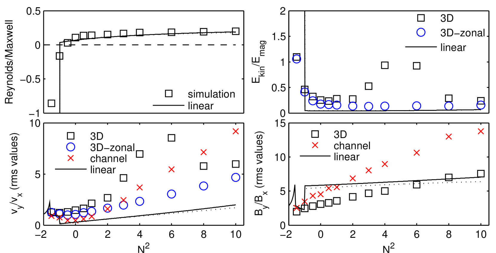
Figure 14: Same as Fig. 13, but high thermal diffusion ($P_{e}=100$).

We found qualitatively similar trends in the case of high thermal diffusion (Fig. 14). In the regime of unstable buoyancy, the Reynolds stress becomes negative and the ratio of kinetic to magnetic energy increases. The ratio of azimuthal to radial velocity and the ratio of azimuthal to radial magnetic field increase significantly with $N^{2}$. Contrary to the low thermal diffusion case, these trends are not reproduced quantitatively, however, by the linear predictions. Still, it is interesting that most qualitative trends are shared between the simulations and the linear modes (e.g. the ratio of azimuthal to radial velocity increases with $N^{2}$), suggesting that linear analysis may still provide a qualitative understanding of these trends.

Finally, Fig. 14 provides interesting information on the coherent channel and zonal flows described in Section 4.1. Our simulations show that the ratios of azimuthal to radial velocity and of azimuthal to radial magnetic field of the quasi-stationary channel flow are quantitatively different from those of the most unstable linear mode (but with a similar qualitative trend). This confirms our conclusion from Section 4.1.1 that quasi-stationary channel flows, while related to MRI modes, have a different structure presumably because they are significantly modified by the concurrent turbulence. The simulations further show that the zonal flows described in Section 4.1.2 are responsible for the bump in kinetic energy observed in Figs. 12 and 14 for $3\lesssim N^{2}/\Omega^{2}\lesssim 6$. Remarkably, at the peak of the zonal flow ($N^{2}/\Omega^{2}=4$ and 6) the kinetic energy is in equipartition with the magnetic energy. Whether this is a mere coincidence or a general property of zonal flows is unclear. Interestingly, if we subtract the contribution of the zonal flow, the remaining kinetic energy (blue circles in the top right panel of Fig. 14) has a smooth flat dependence on $N^{2}$, with no visible impact of the zonal flow (like the total magnetic energy). This suggests that the zonal flow does not significantly impact the level of turbulence developing on top of the zonal flow.

5 Discussion

In this section, we discuss the appropriateness of some of the simplifying assumptions made in our study: use of the Boussinesq approximation (Section 5.1), the assumption of a constant shear rate (Section 5.2), and the local approximation, in particular whether our results depend on the box size (Section 5.3).

5.1 Validity of the Boussinesq approximation

Because our simulations are the first attempt to apply the Boussinesq approximation to the problem of MRI growth in a PNS, it is important to assess to what extent this approximation provides an appropriate description of the flow dynamics. Several conditions should be satisfied for the approximation to be justified. Firstly, the flow velocity and the Alfvén velocity should be much smaller than the sound speed, so that the flow is approximately incompressible. In all our simulations, this requirement holds very well, because $v^{2}/c_{s}^{2}\lesssim v_{A}^{2}/c_{s}^{2}\lesssim 10^{-4}$, the sound speed $c_{s}\simeq 5\times 10^{9}\,{\rm cm\,s^{-1}}$ being estimated from the PNS model studied by Guilet et al. (2015). Secondly, the relative density perturbation associated with buoyancy, $\delta\rho/\rho_{0}=-\theta N^{2}/g$, should be small. Using the gravitational acceleration $g\simeq 6\times 10^{13}\,{\rm cm\,s^{-2}}$ (again from the model of Guilet et al., 2015), we find that in all our simulations its rms value is $\delta\rho/\rho_{0}\lesssim 1.5\times 10^{-3}$, i.e. it is indeed quite small. Thirdly, the Boussinesq approximation neglects the influence of a background density gradient, an assumption that is no longer justified when the size of the box approaches the density scaleheight. For the box size used in our study, the density at the radial surfaces of the box should actually differ from the value at the centre of the box by about $30\%$.

The neglect of the background density gradient is by far the main limitation of the Boussinesq approximation in our simulations. Note that this limitation is common to all local models, even those not employing the Boussinesq approximation (e.g. Masada et al., 2012). It can, in principle, be lifted only by using a global model, or a semi-global model (Obergaulinger et al., 2009). So far, global models resolving the MRI have only been published for two dimensional flows (Sawai et al., 2013; Sawai & Yamada, 2014), which is problematic for a study of MHD turbulence. On the other hand, the inclusion of the density gradient in the semi-global models of Obergaulinger et al. (2009) renders the use of periodic boundary conditions problematic, and causes important artefacts at the radial boundaries of the computational domain (e.g., a fast flattening of the rotation and entropy profiles, which prevents a meaningful study of the non-linear phase of the MRI). The radially global (but vertically local) model of Masada et al. (2015) may not suffer from such boundary artefacts, but the horizontal resolution that they could afford is in our opinion much too coarse for an accurate study of the MRI. We conclude that so far no satisfying solution has been found to study the impact of the large-scale density gradient on the MRI, and that presently the use of local simulations in the Boussinesq approximation is probably the best choice to study the impact of buoyancy on the MRI.

5.2 Energy dissipation rate and timescale of shear profile evolution

Another limitation of local simulations is that they cannot describe the evolution of the global rotation profile. In shearing box simulations with shear-periodic boundary conditions in the radial direction, the shear rate averaged over the box is kept constant. This is justified only as long as the rotation profile has not been significantly modified by the angular momentum transport driven by the MRI.

One can estimate the timescale over which the rotation profile is significantly changed by the ratio of the total available shear energy to the rate at which it is extracted by the combined effects of Reynolds and Maxwell stresses. The available shear energy is estimated in the fast rotating PNS model studied by Guilet et al. (2015) by comparing the rotational energy contained in the differentially rotating PNS to that of a PNS in solid rotation with the same total angular momentum. In this way, we estimate a shear energy of $\sim 4\times 10^{50}\,{\rm erg}$. The specific rate at which energy is extracted from the shear is between $5\times 10^{16}\,{\rm erg\,s^{-1}\,g^{-1}}$ in the regime of stable buoyancy for high thermal diffusion, and $5\times 10^{17}\,{\rm erg\,s^{-1}\,g^{-1}}$ in the unstable buoyancy regime. If we assume that this specific energy extraction rate is uniform in the differentially rotating envelope of the PNS (which contains a mass of $1.6\times 10^{33}\,{\rm g}$ in the PNS model considered), we estimate a total extraction rate of shear energy between $8\times 10^{49}\,{\rm erg\,s^{-1}}$ and $8\times 10^{50}\,{\rm erg\,s^{-1}}$. The typical timescale over which the shear energy is extracted is therefore between $500\,{\rm ms}$ in the unstable buoyancy regime and $5\,{\rm s}$ in the stable one, which is significantly longer than the dynamical timescale $1/\Omega=1\,{\rm ms}$, and also in most cases longer than the time needed to establish the non-linear statistically steady state. This justifies to some extent the relevance of the local approach, but one should keep in mind that in some cases the shear profile should actually have evolved before the end of the simulation.

5.3 Local approximation : dependence on box size

One problem greatly limiting the predictive power of local numerical simulations, is that the result is likely to depend on the size of the computational domain. For the MRI in the absence of buoyancy and in the presence of a vertical magnetic field, numerical simulations have indeed found that the level of turbulence as measured by the angular momentum flux is proportional to the vertical size of the box (Hawley et al., 1995). Since the relevant box size to be adopted is a priori unknown, this renders very uncertain the use of local models to predict magnetic field strength and angular momentum transport in PNS (and casts some doubts on the scaling formulae given by Masada et al. (2012), who did not discuss the dependence of their results on the box size). One may argue the density scale height to be a natural upper limit to the scales available to MRI driven turbulence, such that choosing a local box of a size comparable to the density scale height could be an appropriate choice. Whether this argument actually holds can be checked only with global numerical simulations covering at least several density scale heights if not the whole PNS. While 3D simulations of such global models seem out of reach presently, investigating the dependence of local models on the domain size would already shed more light on its potential impact on the results. The dependence on the box size of MRI simulations that include buoyancy is so far unknown, and should be explored in the future.

6 Conclusions

We have investigated the impact of buoyancy on the properties of the MRI in protoneutron stars. For this purpose, we performed numerical simulations of a local model of a PNS using for the first time the Boussinesq approximation. This approximation has proven very useful to take into account the impact of entropy and lepton number gradients while keeping the advantages of a local model, i.e. clean shearing periodic boundary conditions and low computational cost allowing for an exploration of parameter space. We compared the results of our simulations to those of a linear analysis presented in Appendix A. The main conclusions of our study can be summarized as follows :

• The linear analysis results are confirmed by our numerical simulations: thermal and lepton number diffusion alleviates the stabilising effect of buoyancy, and allows MRI growth in regions of parameter space where the MRI would be stabilised in the absence of diffusion (Menou et al., 2004; Masada et al., 2006, 2007). The growth rate of the MRI is then largely controlled by the thermal and lepton number diffusion, faster diffusion leading to faster MRI growth.

• In the non-linear phase of the MRI, stable buoyancy (i.e. the square of the Brunt-Väisälä frequency $N^{2}>0$) favours the appearance of large scale coherent flows: vertically varying (but horizontally uniform) channel flows as well as radially varying (but azimuthally and vertically uniform) zonal flows. These coherent flows can amount to a significant fraction of the total flow energies. In the case of high thermal diffusion, they are quasi-stationary and very stable over time, while they show recurrent phases of formation and disruption in the case of low thermal diffusion.

• The strength of MHD turbulence (characterized by the magnetic energy or the rate at which energy is injected into turbulence) increases significantly in the regime of unstable buoyancy (i.e. $N^{2}>0$), but it decreases only mildly if the flow is buoyantly stable. This general result is robust, i.e. it holds even when the thermal and lepton number diffusion is varied by a factor ten. The precise variation of turbulence strength with $N^{2}$ does, however, depend on the thermal diffusion. For high diffusion, the magnetic energy decreases monotonically when the flow becomes more and more stable against buoyancy (following the same qualitative trend as the growth rate). In the case of lower diffusion, however, the magnetic energy increases for flows that are very stable against buoyancy, an opposite trend to the growth rate which decreases dramatically. This surprising behaviour is observed in the regime where recurrent channel flows appear, and we speculate that it might be related to the effect of buoyancy on parasitic instabilities growing on MRI channel modes.

• Importantly, we find that the amplitude at which the first exponential growth of the MRI is terminated is not necessarily correlated with the strength of the turbulent phase that follows. Indeed, in the realistic case of high thermal diffusion, the termination amplitude of the MRI increases with $N^{2}$ while the strength of turbulence decreases. This should be kept in mind when interpreting the results of simulations focusing on the MRI termination (Obergaulinger et al., 2009), and highlights the importance of studying the fully turbulent phase of the MRI.

• Other properties of MRI turbulence are strongly influenced by buoyancy. In particular, the ratios of azimuthal to radial magnetic field and of azimuthal to radial velocity increase dramatically in the regime of buoyantly stable flows, where the azimuthal components of the magnetic field and of the velocity therefore dominate the magnetic and kinetic energy. In the regime of buoyantly unstable flows, the ratio of kinetic to magnetic energy increases while the Reynolds stress changes sign and becomes negative. All of these trends are at least qualitatively reproduced by the properties of linear unstable modes.

The magnetic field strength estimated from the volume and time averaged magnetic energy in the non-linear phase of our simulations ranges from $3.5\times 10^{14}\,{\rm G}$ in the case of stable buoyancy with high thermal diffusion to $10^{15}\,{\rm G}$ in the unstable buoyancy regime. Such magnetic field strengths lie the range estimated for magnetars, and they are a few tens to almost a hundred times stronger than the initial magnetic field. This provides support to the ability of the MRI to amplify the initial magnetic field to magnetar strength. Furthermore, if the MRI is at the origin of a magnetar’s magnetic field, our results suggest that the azimuthal magnetic field would be significantly stronger than the poloidal one (in stably stratified regions of the PNS). This could have interesting consequences for magnetars. The observation of magnetar activity from neutron stars with low dipole magnetic field (Rea et al., 2012, 2013, 2014) indicates an internal magnetic field much stronger than its dipolar component. Furthermore, the recent detection of a phase modulation of the pulsed emission of two magnetars has been interpreted as free precession arising from a deformation of the magnetar due to a very strong internal toroidal field (Makishima et al., 2014; Makishima et al., 2015). The generation by the MRI of an azimuthal magnetic field much stronger than its poloidal component could be important to explain these observations.

It has been suggested that the development of the MRI could impact the dynamics of core collapse supernovae explosions (Akiyama et al., 2003) by converting shear energy into thermal energy (Thompson et al., 2005) or by generating large scale magnetic fields that could then drive powerful jet-like explosions (e.g. Moiseenko et al., 2006; Shibata et al., 2006; Burrows et al., 2007; Dessart et al., 2008; Takiwaki et al., 2009; Takiwaki & Kotake, 2011). In the former case, the effect of the MRI was parametrized by an effective turbulent viscosity estimated to reach values up to a few times $10^{13}\,{\rm cm^{2}\,s^{-1}}$ (see Fig. 5 of Thompson et al., 2005). The effective turbulent viscosity can be estimated in our simulations from the angular momentum flux. We found values ranging from $\sim 5\times 10^{10}\,{\rm cm^{2}\,s^{-1}}$ in the stable buoyancy regime with high thermal diffusion to $\sim 5\times 10^{11}\,{\rm cm^{2}\,s^{-1}}$ in the unstable buoyancy regime. These values are two to three orders of magnitude smaller than those used by Thompson et al. (2005), and they would probably not provide enough viscous heating to affect the explosion dynamics. Concerning the second case, the generation of a large scale magnetic field by the MRI cannot be studied in a local model such as ours, and has so far never been demonstrated. Though we could not reach definitive conclusions on this matter, our simulations show that stable buoyancy favours the formation of coherent magnetic structures on the largest scales allowed in our local model. The magnetic field strength we obtained is of the same order of magnitude as that needed to launch jet-driven explosions ($\sim 10^{15}\,{\rm G}$). In order to launch a jet, such a magnetic field strength is, however, needed near the surface of the PNS, while our simulation domain is located deep inside the PNS. Further numerical simulations describing the outer parts of the PNS will therefore be needed to address this question.

We stress that our quantitative conclusions (e.g. strength of the magnetic field, angular momentum flux) should not be considered as definitive answers due to several limitations of our study. Firstly, as discussed in Section 5.3, the results may depend on the size of the computational domain (a limitation shared by all local and semi-global simulations). This size dependence in the presence of buoyancy is unknown so far and should definitely be investigated in future studies. Secondly, the magnetic Prandtl number assumed in our simulations due to numerical constraints ($P_{m}=4$) is much smaller than its realistic value ($P_{m}\sim 10^{13}$). In the absence of buoyancy, MRI turbulence is known to be very sensitive to the magnetic Prandtl number, the strength of turbulence strongly increasing with $P_{m}$ (Lesur & Longaretti, 2007; Fromang et al., 2007; Longaretti & Lesur, 2010). If this trend were to hold in the presence of buoyancy, our results should be considered as lower bounds on the magnetic field strength and the angular momentum flux.

Many questions remain open on the MRI in the presence of buoyancy. As already mentioned, it will be crucial to determine the dependence of our results on the box size and the magnetic Prandtl number. The role of the strength and geometry of the initial magnetic field (both of which are very uncertain) should also be explored. According to models of stellar evolution including magnetic effects approximately, the initial magnetic field might be dominated by its azimuthal component (Heger et al., 2005). Is an efficient amplification of the magnetic field possible, if the initial magnetic field is azimuthal rather than poloidal? How do the results depend on the strength of the initial magnetic field? Further numerical simulations in the framework laid out in this paper could answer such questions. Note also, that this study was restricted to the equatorial plane of the PNS, where the stratification is perpendicular to the rotation axis. It would be interesting to investigate the impact of buoyancy at other latitudes, thereby allowing for a range of angles between the radial stratification and the rotation axis.

Finally, this study was restricted to the inner region of the PNS where neutrinos are in the diffusive regime. Guilet et al. (2015) showed that in the outer parts of the PNS, but still below the neutrinosphere, neutrinos are in the non-diffusive regime on length scales at which the MRI grows. The influence of buoyancy on the MRI in this regime is unknown, and should be studied using both linear analysis and numerical simulations.

Appendix A MHD linear analysis

In this appendix we give an analytical description of the MRI modes growing in the setup described in Section 2. The dispersion relation obtained in Section A.1 is equivalent to that obtained by Menou et al. (2004) and Masada et al. (2007), but restricted to the particular setup considered in this paper, i.e. for a purely vertical magnetic field, the description of buoyancy effects by a single buoyancy variable (relevant to the particular case where the thermal and lepton diffusivities are equal), and considering only the dynamics in the equatorial plane. We repeat the derivation of the respective dispersion relation below, because for our setup the derivation is easier to follow, and because intermediate results (relations between the different velocity and magnetic field components of the modes) are subsequently used in Sections A.2 and A.3.

A.1 dispersion relation

For simplicity, the analysis is restricted to MRI channel modes whose wave vectors are purely vertical (i.e. having only a $z$ component), because these are the fastest growing modes in the presence of a purely vertical background magnetic field. Perturbations from the stationary background flow are assumed to have a time and space dependence $\delta A=Re[\delta\tilde{A}\,e^{\sigma t+ikz}]$ for $A\in\{u_{x},u_{y},u_{z},B_{x},B_{y},B_{z},\theta\}$, where $\sigma$, $k$, and $\delta\tilde{A}$ are the growth rate, the vertical wavevector, and the complex amplitude of the mode, respectively. For conciseness, we drop the $\tilde{}$ symbol when referring to the complex amplitudes in the rest of this section. The equations governing the time evolution of such perturbations are obtained from Eqs. (2.1)–(5). They read

$$\sigma\delta u_{x} = \frac{B_{z}}{4\pi\rho_{0}}ik\delta B_{x}+2\Omega\delta u_{y}-N^{2}\delta\theta-k^{2}\nu\delta u_{x}$$ (31)

$$\sigma\delta u_{y}-\mathrm{S}\delta u_{x} = \frac{B_{z}}{4\pi\rho_{0}}ik\delta B_{y}-2\Omega\delta u_{x}-k^{2}\nu\delta u_{y}$$ (32)

$$\delta u_{z} = 0$$ (33)

$$\sigma\delta B_{x} = B_{z}ik\delta u_{x}-k^{2}\eta\delta B_{x},$$ (34)

$$\sigma\delta B_{y} = B_{z}ik\delta u_{y}-S\delta B_{x}-k^{2}\eta\delta B_{y},$$ (35)

$$\delta B_{z} = 0,$$ (36)

$$\sigma\delta\theta = \delta u_{x}-k^{2}\chi\delta\theta,$$ (37)

where $\mathrm{S}=q\Omega$ is the shear rate with $q$ given by equation (7). Note that these equations are valid for any amplitude of the perturbations, as no linearization had to be done to obtain them. The channel mode solutions that we obtain below are therefore non-linear solutions, just like the classical MRI channel modes in the incompressible limit (Goodman & Xu, 1994). Next, we define

$$\sigma_{\nu}\equiv\sigma+k^{2}\nu,$$ (38)

$$\sigma_{\eta}\equiv\sigma+k^{2}\eta,$$ (39)

$$\sigma_{\chi}\equiv\sigma+k^{2}\chi,$$ (40)

and rewrite Eqs. (31), (32), (34), (35), and (37) as

$$\sigma_{\nu}\delta u_{x} = \frac{B_{z}}{4\pi\rho_{0}}ik\delta B_{x}+2\Omega\delta u_{y}-N^{2}\delta\theta,$$ (41)

$$\sigma_{\nu}\delta u_{y} = \frac{B_{z}}{4\pi\rho_{0}}ik\delta B_{y}-(2\Omega-\mathrm{S})\delta u_{x},$$ (42)

$$\sigma_{\eta}\delta B_{x} = B_{z}ik\delta u_{x},$$ (43)

$$\sigma_{\eta}\delta B_{y} = B_{z}ik\delta u_{y}-S\delta B_{x},$$ (44)

$$\sigma_{\chi}\delta\theta = \delta u_{x}.$$ (45)

Using Eqs. (41) and (43)–(45), one can express all non-vanishing variables as a function of the radial velocity amplitude

$$\delta u_{y}=\frac{1}{2\Omega}\left(\sigma_{\nu}+\frac{N^{2}}{\sigma_{\chi}}+\frac{k^{2}v_{A}^{2}}{\sigma_{\eta}}\right)\delta u_{x},$$ (46)

$$\delta B_{x}=B_{z}\frac{ik\delta u_{x}}{\sigma_{\eta}},$$ (47)

$$\delta B_{y}=\left(\sigma_{\nu}+\frac{N^{2}}{\sigma_{\chi}}+\frac{k^{2}v_{A}^{2}-2\Omega\mathrm{S}}{\sigma_{\eta}}\right)\frac{B_{z}}{\sigma_{\eta}}\frac{ik\delta u_{x}}{2\Omega},$$ (48)

$$\delta\theta=\frac{\delta u_{x}}{\sigma_{\chi}}.$$ (49)

Using equation (42), we then obtain the dispersion relation

$$\sigma_{\chi}\left[\left(\sigma_{\nu}\sigma_{\eta}+k^{2}v_{A}^{2}\right)^{2}+\kappa^{2}\left(\sigma_{\eta}^{2}+k^{2}v_{A}^{2}\right)-4\Omega^{2}k^{2}v_{A}^{2}\right]$$

$$+N^{2}\sigma_{\eta}\left(\sigma_{\nu}\sigma_{\eta}+k^{2}v_{A}^{2}\right)=0,$$ (50)

where $\kappa$ is the epicyclic frequency defined in equation (28). The more general equation (31) of Masada et al. (2007) reduces to our dispersion relation in the case of a purely vertical magnetic field and wavevector, provided the thermal and lepton number diffusivities are equal (in which case our Brunt-Väisälä frequency should be identified with the sum of two frequencies of Masada et al. (2007) that are related to the entropy and lepton number gradient, respectively) or either the lepton number gradient or the entropy gradient vanishes. Equation (50) is also equivalent to equation (13) of Menou et al. (2004), when applied in the equatorial plane to a purely vertical magnetic field and wavevector.

The dispersion relation is a fifth order polynomial in $\sigma$, which can be written in the form

$$a_{5}\sigma^{5}+a_{4}\sigma^{4}+a_{3}\sigma^{3}+a_{2}\sigma^{2}+a_{1}\sigma+a_{0}=0,$$ (51)

with

$$a_{5} = 1,$$ (52)

$$a_{4} = k^{2}\left(\chi+2\nu+2\eta\right),$$ (53)

$$a_{3} = N^{2}+\kappa^{2}+2k^{2}v_{A}^{2}$$ (54)

$$+k^{4}\left[2\chi(\eta+\nu)+4\eta\nu+\nu^{2}+\eta^{2}\right],$$

$$a_{2} = N^{2}k^{2}(\nu+2\eta)+\kappa^{2}k^{2}(\chi+2\eta)$$ (55)

$$+2k^{4}v_{A}^{2}(\nu+\eta+\chi)$$

$$+k^{6}\left[\chi(\nu^{2}+\eta^{2}+4\eta\nu)+2\nu\eta(\eta+\nu)\right],$$

$$a_{1} = k^{8}\left[\eta^{2}\nu^{2}+2\chi(\eta\nu^{2}+\nu\eta^{2})\right]$$ (56)

$$+N^{2}k^{4}(\eta^{2}+2\eta\nu)+\kappa^{2}k^{4}(\eta^{2}+2\eta\chi)$$

$$+k^{2}v_{A}^{2}\left[2k^{4}(\nu\eta+\nu\chi+\eta\chi)+N^{2}\right.$$

$$\phantom{+k^{2}v_{A}^{2}\,}\left.+k^{2}v_{A}^{2}+\kappa^{2}-4\Omega^{2}\right],$$

$$a_{0} = k^{10}\chi\eta^{2}\nu^{2}+N^{2}k^{6}\nu\eta^{2}+\kappa^{2}k^{6}\chi\eta^{2}$$ (57)

$$+k^{2}v_{A}^{2}\left[2k^{6}\nu\eta\chi+N^{2}k^{2}\eta\right.$$

$$\phantom{+k^{2}v_{A}^{2}\,}\left.+(k^{2}v_{A}^{2}+\kappa^{2}-4\Omega^{2})k^{2}\chi\right].$$

In order to obtain the growth rates, this fifth order polynomial is solved numerically using a Laguerre method.

A.2 Reynolds and Maxwell stresses

The vertical average of the Maxwell and Reynolds stresses associated with a channel mode can be computed using the complex amplitudes of the velocity and magnetic field perturbations. The vertical average of the product of two quantities $f$ and $g$ is obtained from their complex amplitudes $\tilde{f}$ and $\tilde{g}$ through

$$\left\langle fg\right\rangle=\frac{1}{L_{z}}\int_{-L_{z}/2}^{L_{z}/2}fg{\rm d}z=\frac{1}{2}{\rm Re}(\tilde{f}\tilde{g}^{*}),$$ (58)

where $\tilde{g}^{*}$ is the complex conjugate of $\tilde{g}$. Here, we have used the relation $Re(z_{1})Re(z_{2})=(z_{1}+z_{1}^{*})(z_{2}+z_{2}^{*})/4=\left[Re(z_{1}z_{2}^{*})+Re(z_{1}z_{2})\right]/2$, for two complex numbers $z_{1}$ and $z_{2}$, and the fact that the vertical average of $Re\left(\tilde{f}\tilde{g}\,e^{2\sigma t+2ikz}\right)$ vanishes (for non vanishing $k$).

Using equation (46), the vertical average of the Reynolds stress reads

$$R_{xy} = Re\left(\sigma_{\nu}+\frac{N^{2}}{\sigma_{\chi}}+\frac{k^{2}v_{A}^{2}}{\sigma_{\eta}}\right)\rho_{0}\frac{|\delta u_{x}|^{2}}{4\Omega}$$ (59)

For an unstable mode ($\sigma>0$) and $N^{2}\geqslant 0$, the Reynolds stress is always positive, which is usually the case for MRI channel modes and turbulence (e.g. Pessah et al., 2006). When $N^{2}\leqslant 0$ on the other hand, the buoyancy can potentially make the Reynolds stress take negative values.

Using Eqs. (47) and (48), we obtain the vertical average of the Maxwell stress

$$M_{xy} = -Re\left[\frac{k^{2}v_{A}^{2}}{\sigma_{\eta}^{2}}\left(\sigma_{\nu}+\frac{N^{2}}{\sigma_{\chi}}+\frac{k^{2}v_{A}^{2}-2\Omega S}{\sigma_{\eta}}\right)\right]$$ (60)

$$\times\rho_{0}\frac{|\delta u_{x}|^{2}}{4\Omega}.$$

Using the dispersion relation, this expression can be rewritten as

$$M_{xy}=Re\left[\frac{\sigma_{\nu}}{\sigma_{\eta}}\left(\sigma_{\nu}+\frac{N^{2}}{\sigma_{\chi}}+\frac{k^{2}v_{A}^{2}}{\sigma_{\eta}}\right)+\frac{\kappa^{2}}{\sigma_{\eta}}\right]\rho_{0}\frac{|\delta u_{x}|^{2}}{4\Omega}.$$ (61)

The same remarks as for the Reynolds stress apply for the Maxwell stress. However, note that the term proportional to $\kappa^{2}$ makes it less likely for the Maxwell stress to become negative, because it would require more negative values of $N^{2}$ than for the Reynolds stress.

A.3 Kinetic and magnetic energies

In a similar way as for the Reynolds and Maxwell stresses, one can obtain the vertically averaged kinetic and magnetic energies

$$E_{K}=Re\left[1+\left(\frac{\sigma_{\nu}+N^{2}/\sigma_{\chi}+k^{2}v_{A}^{2}/\sigma_{\eta}}{4\Omega}\right)^{2}\right]\rho_{0}|\delta u_{x}|^{2},$$ (62)

$$E_{M} = Re\left[1+\left(\frac{\sigma_{\nu}+N^{2}/\sigma_{\chi}+(k^{2}v_{A}^{2}-2\Omega S)/\sigma_{\eta}}{4\Omega}\right)^{2}\right]$$ (63)

$$\times\frac{k^{2}v_{A}^{2}}{Re(\sigma_{\eta}^{2})}\rho_{0}|\delta u_{x}|^{2}.$$

Appendix B Hydrodynamical linear analysis

The dispersion relation in a hydrodynamical flow can be obtained from the MHD dispersion relation by setting the Alfvén velocity to zero in equation (50)

$$\sigma_{\chi}\left(\sigma_{\nu}^{2}+\kappa^{2}\right)+N^{2}\sigma_{\nu}=0.$$ (64)

This third order polynomial in $\sigma$ may be written also in the form

$$a_{3}\sigma^{3}+a_{2}\sigma^{2}+a_{1}\sigma+a_{0}=0,$$ (65)

with

$$a_{3} = 1,$$ (66)

$$a_{2} = k^{2}\chi+2k^{2}\nu,$$ (67)

$$a_{1} = k^{4}\nu^{2}+2k^{4}\nu\chi+\kappa^{2}+N^{2},$$ (68)

$$a_{0} = k^{2}\chi\left(k^{4}\nu^{2}+\kappa^{2}\right)+k^{2}\nu N^{2}.$$ (69)

In order to obtain the growth rates shown in Fig. 3, we solve numerically this third order polynomial using a Laguerre method.

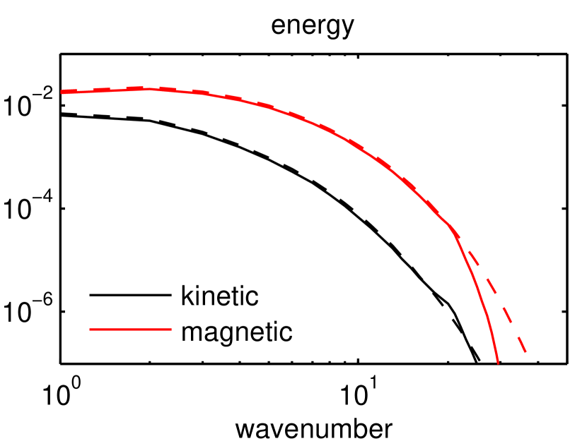
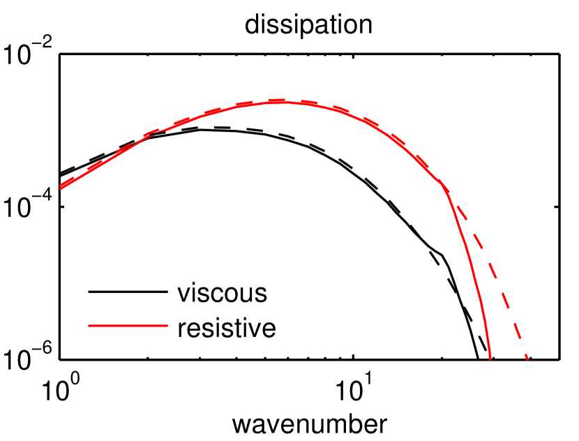
Figure 15: Convergence test for simulations with $N^{2}=0$ and $P_{e}=100$. Results for the standard grid resolution $[n_{x},n_{y},n_{z}]=[256,128,64]$ are shown by solid lines, while results obtained at a twice higher resolution run are shown by dashed lines. Left panel: spectra of the kinetic energy (black lines) and magnetic energy (red lines). Right panel: spectra of the viscous dissipation rate (black lines) and the resistive dissipation rate (red lines). The spectra are averaged over spherical shells in Fourier space following Lesur & Longaretti (2011), and over time for $200\,{\rm ms}\leq t\leq 628\,{\rm ms}$. The wavenumber is normalized to $2\pi/L_{z}$.

An interesting approximate analytical solution of the dispersion relation can be obtained in the inviscid limit by performing an asymptotic expansion for $N^{2}\ll\kappa^{2}$. The zeroth order solution is a simple epicyclic oscillation of frequency $\kappa$ and vanishing growth rate. Performing the expansion up to first order provides the complex growth rate for small $N^{2}$

$$\sigma\simeq i\kappa\left[1+\frac{N^{2}}{2(k^{4}\chi^{2}+\kappa^{2})}\right]-\frac{N^{2}k^{2}\chi}{2(k^{4}\chi^{2}+\kappa^{2})}$$ (70)

where the imaginary part of the growth rate is the oscillation frequency and the real part is the growth rate. The fastest growing mode has the following wavenumber and complex growth rate

$$k_{\rm max}\simeq\sqrt{\kappa/\chi},$$ (71)

$$\sigma\simeq i\kappa\left[1+\frac{N^{2}}{4\kappa^{2}}\right]-\frac{N^{2}}{4\kappa}.$$ (72)

We found this analytical solution to be a rather good approximation in the inviscid limit even for $N^{2}$ of the order of $\kappa^{2}$. The maximum growth rate that we obtain is the same as the one derived by Lyra (2014) for $N^{2}\ll\kappa^{2}$ and a purely vertical wavevector (although these authors considered a thermal relaxation for a given thermal time rather than the diffusion approximation that we used here to describe length scales longer than the neutrino mean free path).

Appendix C Convergence test

We performed a convergence test to check whether the spatial resolution employed in our simulations was sufficient to resolve the dissipation scales, and hence whether the results are unaffected by the limited grid resolution. The spectra of the energy and dissipation rates are shown in Fig. 15 for $N^{2}=0$ and $P_{e}=100$, comparing a run performed with our standard resolution $[n_{x},n_{y},n_{z}]=[256,128,64]$ and a run performed at a twice higher resolution. The energy and dissipation spectra are in good agreement for $kL_{z}/2\pi<20$, i.e. in a regime where most of the energy is located and most of the dissipation occurs. The dissipation rate for $kL_{z}/2\pi>20$ (where the spectra start to differ) is at least an order of magnitude smaller than its peak value. Thus, these unresolved scales have little impact on the dynamics.

When varying the Brunt-Väisälä frequency, we observed for $N^{2}<0$ the peak of the dissipation rate shifted to smaller scales due to the enhanced turbulent activity. We therefore increased the resolution in order to ensure that the peak of viscous, resistive and thermal dissipation is well resolved.

References

- Acheson (1978) Acheson D. J., 1978, Royal Society of London Philosophical Transactions Series A, 289, 459
- Akiyama et al. (2003) Akiyama S., Wheeler J. C., Meier D. L., Lichtenstadt I., 2003, ApJ, 584, 954
- Bai (2014) Bai X.-N., 2014, preprint (arXiv:1409.2511)
- Bai & Stone (2014) Bai X.-N., Stone J. M., 2014, ApJ, 796, 31
- Balbus & Hawley (1991) Balbus S. A., Hawley J. F., 1991, ApJ, 376, 214
- Balbus & Hawley (1994) Balbus S. A., Hawley J. F., 1994, MNRAS, 266, 769
- Bisnovatyi-Kogan et al. (1976) Bisnovatyi-Kogan G. S., Popov I. P., Samokhin A. A., 1976, Ap&SS, 41, 287
- Burrows et al. (2007) Burrows A., Dessart L., Livne E., Ott C. D., Murphy J., 2007, ApJ, 664, 416
- Dessart et al. (2008) Dessart L., Burrows A., Livne E., Ott C. D., 2008, ApJL, 673, L43
- Dessart et al. (2012) Dessart L., Hillier D. J., Waldman R., Livne E., Blondin S., 2012, MNRAS, 426, L76
- Drout et al. (2011) Drout M. R., Soderberg A. M., Gal-Yam A., Cenko S. B., Fox D. B., Leonard D. C., Sand D. J., Moon D.-S., Arcavi I., Green Y., 2011, ApJ, 741, 97
- Duncan & Thompson (1992) Duncan R. C., Thompson C., 1992, ApJL, 392, L9
- Fromang et al. (2007) Fromang S., Papaloizou J., Lesur G., Heinemann T., 2007, A&A, 476, 1123
- Goldreich & Lynden-Bell (1965) Goldreich P., Lynden-Bell D., 1965, MNRAS, 130, 125
- Goodman & Xu (1994) Goodman J., Xu G., 1994, ApJ, 432, 213
- Guilet et al. (2015) Guilet J., Müller E., Janka H.-T., 2015, MNRAS, 447, 3992
- Guilet & Ogilvie (2012) Guilet J., Ogilvie G. I., 2012, MNRAS, 424, 2097
- Guilet & Ogilvie (2013) Guilet J., Ogilvie G. I., 2013, MNRAS, 430, 822
- Hawley et al. (1995) Hawley J. F., Gammie C. F., Balbus S. A., 1995, ApJ, 440, 742
- Heger et al. (2005) Heger A., Woosley S. E., Spruit H. C., 2005, ApJ, 626, 350
- Hirose (2015) Hirose S., 2015, MNRAS, 448, 3105
- Hirose et al. (2014) Hirose S., Blaes O., Krolik J. H., Coleman M. S. B., Sano T., 2014, ApJ, 787, 1
- Inserra et al. (2013) Inserra C., Smartt S. J., Jerkstrand A., et al. 2013, ApJ, 770, 128
- Johansen et al. (2009) Johansen A., Youdin A., Klahr H., 2009, ApJ, 697, 1269
- Kasen & Bildsten (2010) Kasen D., Bildsten L., 2010, ApJ, 717, 245
- Klahr & Hubbard (2014) Klahr H., Hubbard A., 2014, ApJ, 788, 21
- Latter et al. (2009) Latter H. N., Lesaffre P., Balbus S. A., 2009, MNRAS, 394, 715
- LeBlanc & Wilson (1970) LeBlanc J. M., Wilson J. R., 1970, ApJ, 161, 541
- Lesur & Longaretti (2005) Lesur G., Longaretti P.-Y., 2005, A&A, 444, 25
- Lesur & Longaretti (2007) Lesur G., Longaretti P.-Y., 2007, MNRAS, 378, 1471
- Lesur & Longaretti (2011) Lesur G., Longaretti P.-Y., 2011, A&A, 528, A17
- Lesur & Ogilvie (2010) Lesur G., Ogilvie G. I., 2010, MNRAS, 404, L64
- Lesur & Papaloizou (2010) Lesur G., Papaloizou J. C. B., 2010, A&A, 513, A60
- Longaretti & Lesur (2010) Longaretti P.-Y., Lesur G., 2010, A&A, 516, A51
- Lyra (2014) Lyra W., 2014, ApJ, 789, 77
- Makishima et al. (2014) Makishima K., Enoto T., Hiraga J. S., Nakano T., Nakazawa K., Sakurai S., Sasano M., Murakami H., 2014, Physical Review Letters, 112, 171102
- Makishima et al. (2015) Makishima K., Enoto T., Murakami H., Furuta Y., Nakano T., Sasano M., Nakazawa K., 2015, preprint (arXiv:1501.07684)
- Masada et al. (2007) Masada Y., Sano T., Shibata K., 2007, ApJ, 655, 447
- Masada et al. (2006) Masada Y., Sano T., Takabe H., 2006, ApJ, 641, 447
- Masada et al. (2015) Masada Y., Takiwaki T., Kotake K., 2015, ApJL, 798, L22
- Masada et al. (2012) Masada Y., Takiwaki T., Kotake K., Sano T., 2012, ApJ, 759, 110
- Menou et al. (2004) Menou K., Balbus S. A., Spruit H. C., 2004, ApJ, 607, 564
- Metzger et al. (2011) Metzger B. D., Giannios D., Thompson T. A., Bucciantini N., Quataert E., 2011, MNRAS, 413, 2031
- Moiseenko et al. (2006) Moiseenko S. G., Bisnovatyi-Kogan G. S., Ardeljan N. V., 2006, MNRAS, 370, 501
- Mösta et al. (2014) Mösta P., Richers S., Ott C. D., Haas R., Piro A. L., Boydstun K., Abdikamalov E., Reisswig C., Schnetter E., 2014, ApJL, 785, L29
- Müller & Hillebrandt (1979) Müller E., Hillebrandt W., 1979, A&A, 80, 147
- Nicholl et al. (2013) Nicholl M., Smartt S. J., Jerkstrand A., et al. 2013, Nature, 502, 346
- Obergaulinger et al. (2009) Obergaulinger M., Cerdá-Durán P., Müller E., Aloy M. A., 2009, A&A, 498, 241
- Ogilvie & Livio (2001) Ogilvie G. I., Livio M., 2001, ApJ, 553, 158
- Ott et al. (2006) Ott C. D., Burrows A., Thompson T. A., Livne E., Walder R., 2006, ApJS, 164, 130
- Pessah (2010) Pessah M. E., 2010, ApJ, 716, 1012
- Pessah et al. (2006) Pessah M. E., Chan C.-K., Psaltis D., 2006, MNRAS, 372, 183
- Pessah & Goodman (2009) Pessah M. E., Goodman J., 2009, ApJL, 698, L72
- Rea et al. (2012) Rea N., Israel G. L., Esposito P., Pons J. A., Camero-Arranz A., et al. 2012, ApJ, 754, 27
- Rea et al. (2013) Rea N., Israel G. L., Pons J. A., Turolla R., Viganò D., et al. 2013, ApJ, 770, 65
- Rea et al. (2014) Rea N., Viganò D., Israel G. L., Pons J. A., Torres D. F., 2014, ApJL, 781, L17
- Rempel et al. (2010) Rempel E. L., Lesur G., Proctor M. R. E., 2010, Physical Review Letters, 105, 044501
- Sawai & Yamada (2014) Sawai H., Yamada S., 2014, ApJL, 784, L10
- Sawai et al. (2013) Sawai H., Yamada S., Suzuki H., 2013, ApJL, 770, L19
- Shibata et al. (2006) Shibata M., Liu Y. T., Shapiro S. L., Stephens B. C., 2006, Phys. Rev. D, 74, 104026
- Simon & Armitage (2014) Simon J. B., Armitage P. J., 2014, ApJ, 784, 15
- Simon et al. (2012) Simon J. B., Beckwith K., Armitage P. J., 2012, MNRAS, 422, 2685
- Symbalisty (1984) Symbalisty E. M. D., 1984, ApJ, 285, 729
- Takiwaki & Kotake (2011) Takiwaki T., Kotake K., 2011, ApJ, 743, 30
- Takiwaki et al. (2009) Takiwaki T., Kotake K., Sato K., 2009, ApJ, 691, 1360
- Thompson & Duncan (1993) Thompson C., Duncan R. C., 1993, ApJ, 408, 194
- Thompson et al. (2005) Thompson T. A., Quataert E., Burrows A., 2005, ApJ, 620, 861
- Winteler et al. (2012) Winteler C., Käppeli R., Perego A., Arcones A., Vasset N., Nishimura N., Liebendörfer M., Thielemann F.-K., 2012, ApJL, 750, L22
- Woods & Thompson (2006) Woods P. M., Thompson C., 2006, Soft gamma repeaters and anomalous X-ray pulsars: magnetar candidates. pp 547–586
- Woosley (2010) Woosley S. E., 2010, ApJL, 719, L204