S-Wave Superconductivity in Anisotropic Holographic Insulators

Abstract

Within gauge/gravity duality, we consider finite density systems in a helical lattice dual to asymptotically anti-de Sitter space-times with Bianchi VII symmetry. These systems can become an anisotropic insulator in one direction while retaining metallic behavior in others. To this model, we add a $U(1)$ charged scalar and show that below a critical temperature, it forms a spatially homogeneous condensate that restores isotropy in a new superconducting ground state. We determine the phase diagram in terms of the helix parameters and perform a stability analysis on its IR fixed point corresponding to a finite density condensed phase at zero temperature. Moreover, by analyzing fluctuations about the gravity background, we study the optical conductivity. Due to the lattice, this model provides an example for a holographic insulator-superfluid transition in which there is no unrealistic delta-function peak in the normal phase DC conductivity. Our results suggest that in the zero temperature limit, all degrees of freedom present in the normal phase condense. This, together with the breaking of translation invariance, has implications for Homes’ and Uemuras’s relations. This is of relevance for applications to real world condensed matter systems. We find a range of parameters in this system where Homes’ relation holds.

1 Introduction

Significant progress has recently been achieved in applying gauge/gravity duality to strongly coupled systems of relevance to condensed matter physics. In particular, different approaches were proposed to include a lattice into the dual gravity background, in order to holographically study the conductivity in systems with broken translation invariance. Systems with manifest translation invariance display an unrealistic $\delta$-function at zero-frequency in the conductivity; breaking the symmetry weakly broadens this into a realistic Drude peak known from condensed matter physics as a consequence of momentum dissipation. Holography allows moreover the exploration of the consequences of translational symmetry breaking for strongly correlated systems beyond the Drude peak, both in the weak Drude regime and for stronger lattice potentials. We will follow this avenue in the present paper.
Within holography, translation breaking approaches include explicit breaking by a modulated Ansatz for the chemical potential Horowitz2012 ; Liu:2012tr ; Ling:2013aya ; Horowitz2013 , the use of massive gravity Vegh2013 ; Blake:2013owa or linear axions Andrade:2013gsa ; Gouteraux:2014hca ; Taylor:2014tka , or other lattice Ansätze such as the Q-lattices Donos:2013eha or the method used in this work, Bianchi symmetric solutions Iizuka:2012iv ; Iizuka:2012pn . In some cases, translation invariance is also spontaneously broken, for instance when Chern-Simons or $F\wedge F$ terms are present in the gravity action Domokos:2007kt ; Nakamura:2009tf ; Ooguri:2010kt ; Donos:2011bh ; Donos:2013wia ; Withers:2013loa ; Withers:2014sja ; Ling:2014saa , or in an external $SU(2)$ magnetic field Ammon:2011je ; Bu:2012mq . Explicit breaking with an interesting phenomenological consequence is realized in the helical lattice approach Iizuka:2012iv ; Iizuka:2012pn ; Donos2011b ; Donos2012b ; Donos2012a ; Donos2013c ; Donos:2014gya . The original motivation to study this model was that the helical symmetry allows for momentum relaxation along one spatial direction without the need to solve PDEs. The helix in one of the field theory directions along the boundary is encoded in a non-trivial background $U(1)$ gauge field on the gravity side of the holographic duality, and its shape is protected by a so-called Bianchi $\text{VII}_{0}$ symmetry. In addition to that ‘helix $U(1)$’, the five-dimensional gravity action (3) that we study involves a separate ‘charge $U(1)$’ dual to a globally conserved charge current in the boundary theory. This is needed to encode a field theory at finite density. As discussed in Donos2013c , the natural finite density state of this model is a conducting metal, but it can display a transition to an insulating phase as a function of the helix momentum. The remarkable aspect is that this new phase is uni-directional and anisotropic: It is an insulator only along the direction of broken translation invariance along the helical axis. In the orthogonal directions the system remains a metal. From a condensed matter point of view, this system resembles a so-called quantum smectic.
The specific objective we shall be interested in this paper is the consequences of translational symmetry breaking for the transition to superconductivity. This was also recently studied in a holographic Q-lattice in Donos:2013eha ; Ling:2014laa and in axion and related holographic superconductor models in Andrade:2014xca ; Kim:2015dna . In both cases only isotropic models were considered, though both models can support anisotropic lattices Donos:2014uba ; Koga:2014hwa . In our intrinsically anisotropic helical lattice, the dual gravitational dynamics imply that the favored ground state will nevertheless be an isotropic s-wave superconductor. In fact the only Bianchi $\text{VII}_{0}$ symmetric and time-independent Ansatz for the scalar field dual to the order parameter is just a constant in boundary direction. This is the system we shall study. We show that a scalar field added to the helical lattice action and charged under the second $U(1)$ gauge field condenses below a critical temperature, both in the insulating and in the conducting phase. We explore the phase diagram which is determined by the amplitude and the momentum of the translationally symmetry breaking helix, both at finite and at vanishing temperature. Moreover, we analyse the thermodynamical as well as transport properties of the different phases — metallic, insulating, condensed — of the helical lattice model, and obtain the finite temperature phase diagram of the system.
Our findings can be summarized as follows:

The superconducting phase transition: In Section 2 we investigate the finite temperature phase diagram of our model, which displays a second order mean field transition from both the insulating as well as metallic phase to a superfluid phase. We in particular show that the critical temperature $T_{c}$ depends strongly on the amplitude of the helix, but to a first approximation rather weakly on its momentum. This indicates that the strength of the translational symmetry breaking (the depth of the potential wells) is more important than their spatial distribution. For large amplitude, $T_{c}$ can in principle be suppressed all the way to zero, and a quantum phase transition to the uncondensed phase may be expected.
The critical temperature $T_{c}$ does depend mildly on the helix momentum $p$, in a curious way. Starting in the phase at small helix momentum which is originally a zero-temperature insulator in the normal phase, $T_{c}$ decreases with increasing helix momentum. However, $T_{c}$ grows again for even larger helix momentum. This might be understood from the observation that initially with increasing momentum the underlying original insulating system changes to a zero temperature conductor in the normal phase, but then for even larger momentum turns back into an insulator.

The optical conductivity: In Section 3 we calculate the optical conductivity in the direction of translational symmetry breaking in the insulating, conducting as well as condensed phases. In the insulating and conducting phases we reproduce the results of Donos2013c . In the condensed phase we observe the appearance of a gap at low frequencies as expected for spontaneous symmetry breaking. The spectral weight is transferred to a $\delta$-function contribution at zero frequency: this is confirmed with the Ferrell-Glover-Tinkham sum rule.
The virtue of the helix model is that this $\delta$-function is now cleanly interpreted as the consequence of spontaneous symmetry breaking. There is no artificial contribution due to translational symmetry. The strength of this $\delta$-peak therefore defines the superfluid density in the condensed phase. For weak momentum relaxation, $\nicefrac{{\lambda}}{{\mu}}\ll 1$ we find that in the limit $T\rightarrow 0$, the superfluid density coincides with the total charge density in the system, as measured by the second $U(1)$ gauge field. This can be understood by the fact that the zero-temperature normal state of our system is already in a cohesive phase, in which no uncondensed charged degrees of freedom are present in the deep IR. This however does not mean that we are dealing with a plain vanilla superconductor. At any finite temperature, the horizon does carry charge. This reflects itself in the temperature dependence of the superconducting gap. We find that the low $T$ behavior of the superconducting gap is algebraic, i.e. $\sigma(\omega^{\ast})\sim T^{\#}$, rather than exponential. Nevertheless as stated earlier, computing the thermodynamical charge density $n_{s}$ and the superfluid density $\rho_{s}$ independently, we find that they coincide in the limit of zero temperature, in the regime of weak momentum relaxation.
The helical system considered has therefore two important properties: Translation symmetry is broken and all charged degrees of freedom condense at very low temperatures. The combination of both these facts enables us to take a further look at Homes’ relation in the context of holography. This empirical law, found experimentally Homes2004 ; Homes2005 , states that there is a universal behaviour for classes of superconductors that relates the superconducting density $\rho_{s}$ at zero temperature to the DC conductivity $\sigma_{\mathrm{DC}}$ at $T_{c}$

$$\rho_{s}(T=0)=C\sigma_{\mathrm{DC}}(T_{c})\cdot T_{c}.$$ (1)

The constant $C$, which is dimensionless in suitable units, is experimentally found to be around $C=4.4$ for in-plane high-$T_{c}$ superconductors as well as clean BCS superconductors and around $C=8.1$ for c-axis high-$T_{c}$ materials and BCS superconductors in the dirty limit Homes2004 ; Homes2005 . Generally, a relation of this type is expected for systems which are Planckian dissipators Zaanen2004 . Homes’ relation was first considered in the context of holography in Erdmenger2012a , where it was found that for a holographic realization, both translation symmetry breaking and the condensation of all charged degrees of freedom are necessary conditions. Both of these conditions are realized in the helical lattice system in the present paper. It was found in Horowitz2013 that a simple breaking of translation invariance by a modulated chemical potential is not sufficient for a holographic realization of Homes’ relation, essentially since in the limit of vanishing chemical potential, the DC conductivity diverges while the superconducting density remains finite. Indeed, Homes’ relation cannot hold for weak momentum relaxation. However, motivated by the arguments given above, we considered Homes’ relation in the context of the helical lattice model for strong momentum relaxation. In a parameter region around the minimum of $T_{c}$ found in Section 2, $C$ appears to be roughly constant for a significant region in parameter space. We find a value of about

$$C=6.2\pm 0.3,$$ (2)

which lies between the experimental results for high $T_{c}$ and dirty limit BCS superconductors. These encouraging results call for further detailed analysis, which we leave for future work.

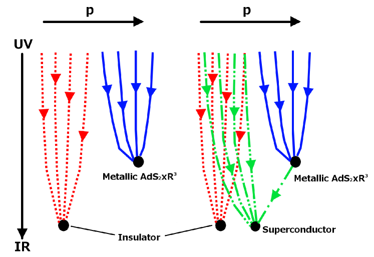
Figure 1: Sketch of the holographic renormalisation group flows without (left panel) and with superconducting order parameter (right panel), for the case of large $\kappa\geq 0.57$ in which no additional unstable bifurcation fixed points appear in the model of Donos2013c . Without the superconducting order parameter, the transition from the insulating (red dotted) to the metallic $\text{AdS}_{2}\times\mathds{R}^{3}$ (blue solid) ground states occurs as the helix pitch $\nicefrac{{p}}{{\mu}}$ is increased Donos2013c . With the superconducting order parameter a new superconducting (green dash-dot-dotted) ground state, (63), appears. While the metallic ground states becomes dynamically unstable and presumably flows to the superconductor, the insulating states stay dynamically stable but are presumably thermodynamically disfavoured compared to flows to the superconducting fixed point.

The zero-temperature ground state: In Section 4 we provide a preliminary analysis of the zero-temperature ground states of the condensed system. The starting point is the IR geometry of the insulating ground state geometry of the helical model in the absence of a condensate Donos2013c . We show that this Ansatz for the IR geometry can naturally be extended to the superconducting solution. Besides this, the insulating as well as metallic ground states of Donos2013c continue to exist. We perform the usual IR fluctuation analysis and delineate the various IR relevant directions, if present, and the IR irrelevant directions. This allows us to understand the RG flow of the model in principle (Figure 1). We in particular find a difference in the instability mechanisms of the insulating and metallic fixed points of Donos2013c : While the metallic $\text{AdS}_{2}\times\mathds{R}^{3}$ becomes dynamically unstable at low temperatures towards condensation of the superconducting order parameter, the insulating fixed point stays dynamically stable, but most presumably becomes thermodynamically disfavored compared with flows to the superconducting fixed point. Since our finite temperature phase diagram (Figure 5) indicates the possibility of a zero temperature phase transition between the condensed and insulating solution, these results calls for a more detailed study of the phase diagram at finite and zero temperature in a future work WIP .

We conclude in Section 5 where we discuss in particular the implications of our results for the holographic realization of Homes’ relation. We end by giving an outlook to further investigations.

2 Holographic S-Wave Superconductors on a Helical Lattice

In this section we first explain our setup, which is based on the model of Donos2013c . We then discuss and present our results for the finite temperature phase diagram.

2.1 Holographic Setup

The holographic model that dualizes to a field theory in the presence of a helical lattice has the action Donos2013c

$$S_{\text{helix}}={} \int\operatorname{d^{4+1}\mathit{x}}\sqrt{-g}\bigg{[}R+12-\frac{1}{4}F^{\mu\nu}F_{\mu\nu}-\frac{1}{4}W^{\mu\nu}W_{\mu\nu}-m^{2}B_{\mu}B^{\mu}\bigg{]}$$

$$-\frac{\kappa}{2}\int B\wedge F\wedge W.$$ (3)

Here $g_{\mu\nu}$ is the metric of a 5-dimensional asymptotically anti-de-Sitter spacetime including the $3+1$ field theory dimensions and the additional radial coordinate $r$. $R$ is the Ricci scalar of this metric. There are two field strengths: $F_{\mu\nu}=\partial_{\mu}A_{\nu}-\partial_{\nu}A_{\mu}$ is the Maxwell field which accounts for the $U(1)$ charge dynamics. The additional massive Proca field $B_{\mu}$ generates the ‘helix U(1)’ with field strength $W_{\mu\nu}=\partial_{\mu}B_{\nu}-\partial_{\nu}B_{\mu}$, and supports the helical structure. In addition, there is a Chern-Simons term which couples the fields $A_{\mu}$ and $B_{\mu}$ with coupling constant $\kappa$. In the above action, the AdS radius $L$ has been set to one. Furthermore, Newton’s constant has been fixed to $\kappa_{5}^{2}=1/2$. This can be achieved by redefining the remaining couplings such that $\nicefrac{{1}}{{(2\kappa_{5}^{2})}}$ becomes a total factor multiplying the action.
To encode the $U(1)$ order parameter, we add to this action a scalar field with charge $q$ and mass $m_{\rho}$ minimally coupled to $A_{\mu}$,

$$S_{\text{total}}=S_{\text{helix}}+ \int\operatorname{d^{4+1}\mathit{x}}\sqrt{-g}\bigg{[}-|\partial\rho-\mathrm{i}qA\rho|^{2}-m_{\rho}^{2}|\rho|^{2}\bigg{]}.$$ (4)

The equations of motion following from the action (4) are

$$R_{\mu\nu}-\frac{1}{2}Rg_{\mu\nu}-6g_{\mu\nu}=T^{(A)}_{\mu\nu}+T^{(B)}_{\mu\nu}+T^{(\rho)}_{\mu\nu},$$ (5)

where

$$T^{(A)}_{\mu\nu} =\frac{1}{2}F_{\mu\alpha}F\indices{{}_{\nu}^{\alpha}}-\frac{1}{8}g_{\mu\nu}F^{2}$$

$$T^{(B)}_{\mu\nu} =\frac{1}{2}W_{\mu\alpha}W\indices{{}_{\nu}^{\alpha}}-\frac{1}{8}g_{\mu\nu}W^{2}-\frac{m^{2}}{2}B_{\mu}B_{\nu},$$

$$T^{(\rho)}_{\mu\nu} =\operatorname{Re}\big{[}(\nabla_{\mu}\rho^{\ast}+\mathrm{i}qA_{\mu}\rho^{\ast})(\nabla_{\nu}\rho-\mathrm{i}qA_{\nu}\rho)\big{]}-\frac{1}{2}g_{\mu\nu}\big{(}|\partial\rho-\mathrm{i}qA\rho|^{2}+m_{\rho}^{2}|\rho|^{2}\big{)},$$ (6)

are the energy-momentum tensors of the two vector fields $A$ and $B$, and of the complex scalar $\rho$. Furthermore, we have the scalar equation

$$0 =\left[(\nabla^{\mu}-\mathrm{i}qA^{\mu})(\nabla_{\mu}-\mathrm{i}qA_{\mu})-m_{\rho}^{2}\right]\rho,$$ (7)

and the Maxwell equations

$$\nabla_{\mu}F^{\mu\nu} =\mathrm{i}q\left[\rho^{\ast}(\partial^{\nu}-\mathrm{i}qA^{\nu})\rho-\rho(\partial^{\nu}+\mathrm{i}qA^{\nu})\rho^{\ast}\right]+\frac{\kappa}{4\sqrt{-g}}\tilde{\epsilon}^{\mu\nu\alpha\beta\gamma}\partial_{\alpha}(B_{\mu}W_{\beta\gamma}),$$ (8)

$$\nabla_{\mu}W^{\mu\nu} =m^{2}B^{\nu}+\frac{\kappa}{8\sqrt{-g}}\tilde{\epsilon}^{\mu\nu\alpha\beta\gamma}\left[2\partial_{\gamma}(B_{\mu}F_{\alpha\beta})-F_{\mu\alpha}W_{\beta\gamma}\right].$$ (9)

Here $\tilde{\epsilon}^{\mu\nu\alpha\beta\gamma}$ is the totally antisymmetric Levi-Civita symbol in 5 dimensions with $\tilde{\epsilon}^{01234}=1$. As in Donos2013c , the wedge product in the action (4) is normalized such that the Chern-Simons term evaluated on the chosen Ansatz equals $S_{\text{CS}}=\int dr\,p\kappa w^{2}a^{\prime}/2$. We now construct solutions to the equations that have the following properties. First we aim to study the system with the helix structure in order to break translational symmetry. For this purpose, the one-forms

$$\omega_{1} =\operatorname{d\mathit{x}}\text{,}$$

$$\omega_{2} =\cos(px)\operatorname{d\mathit{y}}-\sin(px)\operatorname{d\mathit{z}},$$

$$\omega_{3} =\sin(px)\operatorname{d\mathit{y}}+\cos(px)\operatorname{d\mathit{z}},$$ (10)

are introduced. They provide a basis for the spatial $(x,y,z)$ part of the metric and the two vector fields $A_{\mu}$ and $B_{\mu}$. In Figure 2, one period of $\omega_{2}$ is plotted along the $x$-coordinate. The forms $\omega_{2}$ and $\omega_{3}$ have the structure of a helix with periodicity $\nicefrac{{2\pi}}{{p}}$.

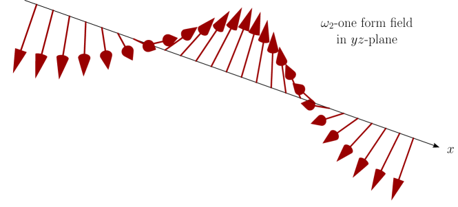
Figure 2: Plot of the one-form $\omega_{2}$ along the $x$-axis for one period. Being periodic with period $2\pi/p$, $\omega_{2}$ is not translationally invariant for $p\neq 0$. The vector field $B=w(r)\omega_{2}$ acts as a source for the helix and imprints the helical, translational symmetry breaking structure on the system.

In the following, we focus on the case $m=0$, i.e. we are considering a massless helix field $B$. In our setup, the role of $B$ is to introduce a lattice in a phenomenological way and thus break translational symmetry. Since this can be achieved with a massless helix field, $m=0$ is chosen for simplicity. This choice follows Donos2013c . Using these one-forms we make the Ansatz for the helix field $B=B_{\mu}dx^{\mu}$ to be

$$B =w(r)\omega_{2}, \qquad\qquad w(\infty) =\lambda,$$ (11)

where $r=\infty$ denotes the boundary of the asymptotically anti-de-Sitter space. Since this Ansatz shows that $B_{y}$ and $B_{z}$ do not vanish at the boundary, the field theory interpretation is that we explicitly introduce a source $\lambda$ for the operator dual to $B$, i.e. we are deforming the homogeneous theory by a lattice operator. $\lambda$ can be interpreted as the lattice strength. The field $B$ extends along $\omega_{2}$ and therefore breaks translational symmetry in the $x$-direction for $p\neq 0$. Via backreaction on the metric, this helical structure is imprinted on the whole gravitational system. This is manifested in a metric Ansatz Iizuka:2012iv

$$\operatorname{d\mathit{s}}^{2}=-U(r)\operatorname{d\mathit{t}}^{2}+\frac{\operatorname{d\mathit{r}}^{2}}{U(r)}+\,\mathrm{e}^{2v_{1}(r)}\,\omega_{1}^{2}+\,\mathrm{e}^{2v_{2}(r)}\,\omega_{2}^{2}+\,\mathrm{e}^{2v_{3}(r)}\,\omega_{3}^{2}.$$ (12)

From a technical point of view, the usefulness of this Ansatz is that it is compatible with the so-called Bianchi $\text{VII}_{0}$ symmetry and is therefore guaranteed to be self-consistent — naïvely the spatial dependence in the one-forms should imply that all the components of the metric become spatially dependent. Thanks to the symmetry this is not so. Instead, all $x$-dependence is carried by the one-forms of Eq. (10) such that the resulting equations of motion are ordinary differential equations in the radial coordinate $r$. It is therefore consistent to assume that all fields are functions of $r$ only, even though translational symmetry is broken. In the dual field theory the blackening factor $U$ encodes the energy density and the $v_{i}$ are related to the pressures in the system. In the finite temperature phase, the metric function $U$ has a zero at a finite value of $r$, which defines the thermal horizon radius $r_{h}$,

$$U(r_{h})=0.$$ (13)

We will consider solutions which, for large values of $r$, satisfy

$$U(r) =r^{2}+\ldots, \qquad\qquad v_{i}(r) =\ln(r)+\ldots, \qquad\qquad\text{for }i =1,2,3.$$ (14)

This guarantees that at the boundary (for $r\to\infty$) the metric is of anti-de Sitter form, $\operatorname{d\mathit{s}}^{2}=\operatorname{d\mathit{r}}^{2}/r^{2}+r^{2}(-\operatorname{d\mathit{t}}^{2}+\operatorname{d\mathit{\mathbfit{x}}}^{2})$. Field theoretically, this means that the theory has an ultraviolet fixed point with conformal symmetry. The introduction of the helix through the source for the operator dual to $B_{\mu}$ deforms away from this UV fixed point, as we will see below, c.f. Eq. (39). To model a field theory at finite density, we make the additional Ansatz

$$A =a(r)\operatorname{d\mathit{t}}, \qquad\qquad a(\infty) =\mu.$$ (15)

Field theoretically the operator dual to $A_{\mu}$ is a conserved current $j^{\mu}$. As this Ansatz again does not vanish at the AdS boundary it means that we introduce a source for the zero component of $j^{\mu}$. We work in the grand canonical ensemble with chemical potential $\mu$ rather then a system at fixed density. We furthermore choose the charged scalar, which is the gravitational encoding of our superconducting order parameter, to respect the Bianchi VII₀ symmetry, i.e. to be invariant under the vector fields dual to the Bianchi VII₀ one-forms in Eq. (10),

$$\omega_{i}^{\mu}\partial_{\mu}\rho(t,x,y,z,r) =0, \qquad i =1,2,3.$$ (16)

Since the Bianchi one-forms (10) are linearly independent, this restricts the charged scalar to be at most of form $\rho(t,r)$. For the background we choose a time-independent Ansatz $\rho(r)$. Note that choosing a superconducting order parameter compatible with the helix symmetries corresponds, in condensed matter terminology, to the statement that the superconducting order parameter must respect the crystal symmetry of the underlying lattice. The resulting coupled ordinary differential equations for the functions $a$, $w$, $U$, $v_{1}$, $v_{2}$, $v_{3}$ and $\rho$ can be found in Appendix A. Making use of the $U(1)$ symmetry associated with $A_{\mu}$, $\rho$ is chosen to be real. The total differential order of the equations of motion is 13, corresponding to the three second order equations for $a,w$ and $\rho$, three second order Einstein equations and one first order Einstein equation, the constraint equation. It will be shown that this system exhibits a second order phase transition at finite temperature: above some critical temperature $T_{c}$, the system is in a state with a vanishing scalar field; below $T_{c}$ a phase with a non-vanishing scalar field is thermodynamically preferred. The order parameter of the phase transition is the vacuum expectation value $\Braket{\mathcal{O}_{\rho}}$ of the operator dual to $\rho$, and the low temperature phase is characterized by breaking the global $U(1)$ under which $\mathcal{O}_{\rho}$ is charged. Since we will only consider the case of $\mathcal{O}_{\rho}$ not being sourced explicitly, the $U(1)$ symmetry is broken spontaneously. The superconducting phase transition can be understood in terms of an effective scalar mass becoming sufficiently negative: from the scalar field equation

$$0=\rho^{\prime\prime}+\rho^{\prime}\left(\frac{U^{\prime}}{U}+v_{1}^{\prime}+v_{2}^{\prime}+v_{3}^{\prime}\right)+\rho\left(\frac{a^{2}q^{2}}{U^{2}}-\frac{m_{\rho}^{2}}{U}\right),$$ (17)

we can deduce the effective $r$-dependent scalar mass $m_{\text{eff}}^{2}={m_{\rho}^{2}-q^{2}a^{2}}/U$. The second term shifts the effective mass squared towards smaller values and causes an instability as $m_{\text{eff}}^{2}$ becomes sufficiently negative. Both larger values of $q$ and more negative values of $m_{\rho}^{2}$ favor the appearance of the instability. Most studies on holographic superconductors with a scalar condensate focus on tachyonic scalar masses corresponding to relevant operators. From studies on translationally invariant s-wave superconductors it is however known that condensation to a superconducting state also appears for a massless (and even irrelevant) scalar Horowitz2008 . As in the case of translationally invariant s-wave superconductors studied in Horowitz2009 , it is expected that the zero temperature infrared geometry depends on the mass of the scalar field and that the massless scalar represents one of several distinct cases. In the following, we focus on the case $m_{\rho}=0$ and leave the case of general scalar masses to further studies. One reason for this choice will become clear in Section 4: We have only been able to construct extremal (zero temperature) geometries for this value of the scalar mass. The mass of the scalar field $m_{\rho}$ is related to the scaling dimension $\Delta$ of the operator dual to $\rho$ via $\Delta=2+\sqrt{4+m_{\rho}^{2}}$. Therefore, the case $m_{\rho}=0$ corresponds to a marginal operator with $\Delta=4$. The Chern-Simons term couples the Maxwell field $A_{\mu}$ and the helix field $B_{\mu}$. The authors of Donos2013c point out that in their case the Chern-Simons coupling allows for the existence of a cohesive phase, i.e. a phase without electric flux through the horizon. This requires some field or coupling that sources the electric field outside of the horizon. The insulating geometry of Donos2013c is of this type and it is stabilized by the Chern-Simons interaction, inducing the necessary charge density via the coupling to the helix field. In particular, for larger values of the Chern-Simons coupling $\kappa>0.57$ Donos2013c the phase diagram simplifies due to the absence of an under RG flow unstable bifurcation critical point. Due to this added simplicity, and in order to be compatible with the results of Donos2013c , we focus in this work on the case of relatively large Chern-Simons coupling and choose $\kappa=\nicefrac{{1}}{{\sqrt{2}}}$. Furthermore, in order to be able to compare the physics of our model better to the usual holographic superconductor Hartnoll2008 ; Hartnoll2008a , we also investigate the case of vanishing Chern-Simons coupling $\kappa=0$.

2.1.1 Asymptotic Expansions

As an important step towards solving the equations of motion, asymptotic expansions are calculated at the thermal horizon $r_{h}$ and at the boundary, i.e. for large values of $r$. These are the two points where the boundary conditions on the fields are imposed. In addition to its defining property as the zero of the metric function $U$, the horizon $r_{h}$ is also a zero of the Maxwell potential $a$ due to regularity (c.f. for example Horowitz2011 )

$$U(r_{h}) =0, a(r_{h}) =0.$$ (18)

The remaining fields are finite at the horizon. At the boundary $$r\to\infty$$, the conditions

$$a =\mu, \qquad\qquad w =\lambda, \qquad\qquad\rho =0, \qquad\qquad v_{i} =\ln(r),$$ (19)

are imposed. The first three conditions determine the sources of the operators dual to $a,w$ and $\rho$. For general scalar field masses $m_{\rho}$, the leading power of $\rho$ at the boundary is $r^{-(4-\Delta)}$, where $\Delta$ is the scaling dimension of $\rho$. The massless scalar considered here has $\Delta=4$, such that it is constant to leading order in $\nicefrac{{1}}{{r}}$. Therefore, the source of the operator dual to $\rho$ is chosen to vanish by imposing $\rho=0$ at the boundary. A solution with a non-vanishing scalar field in the bulk then breaks the $U(1)$ symmetry associated with the Maxwell field spontaneously. As discussed before, the conditions on $v_{i}$ ensure that the metric is asymptotically anti-de Sitter. For an asymptotically AdS space it is also required that $U(r)=r^{2}$ at the boundary. This condition, however, follows from the equations of motion (in particular the constraint, the sixth line in (82)) and does not need to be imposed explicitly. In order to determine the asymptotic horizon expansion respecting the conditions stated above, we make the Ansatz

$$a =a^{h}_{1}(r-r_{h})+a^{h}_{2}(r-r_{h})^{2}+\dotsb, \qquad w =w^{h}_{0}+w^{h}_{1}(r-r_{h})+\dotsb,$$ (20)

$$U =U^{h}_{1}(r-r_{h})+U^{h}_{2}(r-r_{h})^{2}+\dotsb, v_{i} =v^{h}_{(i,0)}+v^{h}_{(i,1)}(r-r_{h})+\dotsb,$$

$$\rho =\rho^{h}_{0}+\rho^{h}_{1}(r-r_{h})+\dotsb,$$

and solve the equations of motion order by order in $r-r_{h}$. The horizon expansion has seven free parameters which are chosen to be

$$(a^{h}_{1},w^{h}_{0},\rho^{h}_{0},U^{h}_{1},v^{h}_{(i,0)}).$$ (21)

All higher order expansion coefficients can be expressed in terms of these parameters. $U^{h}_{1}$ is related to the Hawking temperature by

$$T=\frac{U^{\prime}(r_{h})}{4\pi}=\frac{U^{h}_{1}}{4\pi}.$$ (22)

The asymptotic horizon expansion will be used to define initial conditions for the numerical integration of the equations of motion. At the boundary, a double expansion in $\nicefrac{{1}}{{r}}$ and in $\nicefrac{{\ln(r)}}{{r}}$ is carried out. The $\ln(r)$-terms introduce a scale and indicate the presence of a scaling anomaly, which is related to the lattice structure. This will be discussed in more detail in Section 2.1.2, where the stress-energy tensor of the system is calculated. The following Ansatz is used as a building block for the asymptotic expansion at the boundary

$$f_{N}(r)={} \sum^{N}_{k=0}\sum^{N-k}_{j=0}a_{k,j}\left(\frac{1}{r}\right)^{k}\left(\frac{\ln r}{r}\right)^{j}$$

$$={} a_{00}+\left(a_{10}\frac{1}{r}+a_{01}\frac{\ln r}{r}+\dotsb\right)$$

$$+\left(a_{20}\frac{1}{r^{2}}+a_{11}\frac{\ln r}{r^{2}}+a_{02}\frac{(\ln r)^{2}}{r^{2}}+\dotsb\right)+\dotsb.$$ (23)

The constant $N$ defines the order of the expansion. Since both $\nicefrac{{1}}{{r}}$ and $\nicefrac{{\ln(r)}}{{r}}$ are small for large values of $r$, higher powers in the expansion are truly subleading. $f_{N}(r)$ is used to define an Ansatz for the matter fields $a,w$ and $\rho$. The Ansatz for $U$ is given by $r^{2}f_{N}(r)$, and the Ansatz for the metric functions $v_{i}$ by $\ln(r)+f_{N}(r)$. This accounts for the fact that $r^{2}$ is the leading behavior of $U$ and of $\,\mathrm{e}^{2v_{i}}\,$ for large values of $r$. Solving the equations of motion order by order in $\nicefrac{{1}}{{r}}$, we obtain an asymptotic expansion with the leading terms

$$a =\mu+\frac{\nu}{r^{2}}+\dotsb, \qquad w =\lambda+\frac{\beta-p^{2}\lambda\,{\ln(r)}/2}{r^{2}}+\dotsb,$$ (24)

$$U =r^{2}-\frac{\epsilon/3+p^{2}\lambda^{2}\,{\ln(r)}/6}{r^{2}}+\dotsb, v_{1} =\ln(r)+\frac{g_{1}+p^{2}\lambda^{2}\,{\ln(r)}/{24}}{r^{4}}+\dotsb,$$

$$v_{2} =\ln(r)+\frac{g_{2}-p^{2}\lambda^{2}\,{\ln(r)}/{12}}{r^{4}}+\dotsb, v_{3} =\ln(r)+\frac{g_{3}+p^{2}\lambda^{2}\,{\ln(r)}/{24}}{r^{4}}+\dotsb,$$

$$\rho =\frac{\rho_{b}}{r^{4}}-\frac{q^{2}\mu^{2}\rho_{b}}{12r^{6}}+\dotsb.$$

Here we find that $g_{3}$ satisfies

$$g_{3}=-g_{1}-g_{2}.$$ (25)

As we will see later, the parameters $g_{i}$ are related to the pressure of the system and $\epsilon$ is the energy density. The subleading mode of $a$ denoted by $\nu$, is related to the charge density and $\beta$, the subleading mode of $w$, to the vacuum expectation value of the operator dual to $w$. The leading mode of $\rho$ has been set to zero and the subleading mode, $\rho_{b}$, is proportional to the vacuum expectation value $\Braket{\mathcal{O}_{\rho}}$. In total there are 8 physical parameters at the boundary, namely

$$(\epsilon,g_{1},g_{2},\mu,\nu,\lambda,\beta,\rho_{b}).$$ (26)

There is another, non-physical parameter present in the asymptotic boundary expansion, which has been set to zero above to keep the expressions clear. This parameter is related to a shift in the $r$ coordinate. It can be reinstated into the boundary expansion by the transformation

$$r \to r+\frac{\alpha}{2}, g_{1} \to g_{1}+\frac{\alpha^{4}}{64}, g_{2} \to g_{2}+\frac{\alpha^{4}}{64}.$$ (27)

$\alpha$ gives rise to odd powers of $\nicefrac{{1}}{{r}}$ in the boundary expansion. These odd powers are in general present in the (numerical) solutions to the equations of motion. However, in contrast to the remaining parameters of the asymptotic expansion, $\alpha$ has no physical meaning. It can be thought of as an artifact of the coordinate choice. Note that the Ansatz of Eq. (12), and therefore also the equations of motion, do not explicitly depend on the radial coordinate $r$. As a consequence, the system exhibits a shift-symmetry $r\to r+\text{const.}$ in the radial direction. The presence of $\alpha$ in the boundary expansion reflects precisely this shift-symmetry.

2.1.2 Thermodynamics and the Conformal Anomaly

The temperature of our strongly coupled field theory is given by the Hawking temperature of the bulk black hole, Eq. (22). The Bekenstein-Hawking entropy is calculated according to the area law as

$$S =4\pi A_{h}=4\pi\int\operatorname{d\mathit{\tau}}\operatorname{d^{3}\mathit{\mathbfit{x}}}\sqrt{\gamma}\bigg{|}_{r\to r_{h}}=4\pi\,\mathrm{e}^{v_{1}(r_{h})+v_{2}(r_{h})+v_{3}(r_{h})}\,V.$$ (28)

Here $A_{h}$ denotes the area of the black hole horizon, $\gamma_{ab}$ is the induced metric and $V=\int\operatorname{d^{3}\mathit{\mathbfit{x}}}$ denotes the $3$-dimensional volume of the field theory. In order to determine the grand canonical potential, we calculate the Euclidean (imaginary time) on-shell action. Applying appropriate integrations by part with respect to $r$, the Euclidean action reduces to a boundary term upon use of the equations of motion. We obtain the two versions

$$I_{\text{bulk}} =\frac{V}{T}\left[-a\,\mathrm{e}^{v_{1}+v_{2}+v_{3}}\,a^{\prime}-\frac{1}{2}a\kappa pw^{2}+\,\mathrm{e}^{v_{1}+v_{2}+v_{3}}\,U^{\prime}\right]^{r=r_{b}}_{r=r_{h}},$$

$$I_{\text{bulk}} =\frac{V}{T}\left[\frac{1}{2}U\,\mathrm{e}^{v_{1}-v_{2}+v_{3}}\,ww^{\prime}+U\,\mathrm{e}^{v_{1}+v_{2}+v_{3}}\,v_{2}^{\prime}+U\,\mathrm{e}^{v_{1}+v_{2}+v_{3}}\,v_{3}^{\prime}\right]^{r=r_{b}}_{r=r_{h}},$$ (29)

which will give rise to two expressions for the grand canonical potential $\Omega$. A regularizing ultraviolet cutoff $r_{b}\gg r_{h}$ has been introduced. Eventually, after determining appropriate counterterms, the limit $r_{b}\to\infty$ will be taken. The renormalized Euclidean on-shell action is given by $I_{\text{os}}=I_{\text{bulk}}+I_{\text{GH}}+I_{\text{ct}}$, where $I_{\text{GH}}$ is the Gibbons-Hawking boundary term and $I_{\text{ct}}$ stands for the counterterms necessary to make $I_{\text{os}}$ finite. The factor $\nicefrac{{1}}{{T}}=\beta$ originates from the $\tau$-integration and $V=\int\operatorname{d^{3}\mathit{\mathbfit{x}}}$ is the three-dimensional volume. Note that the second expression for $I_{\text{bulk}}$ receives no contribution from the horizon since $U(r_{h})=0$. The Gibbons-Hawking term is evaluated as

$$I_{\text{GH}} =-2\int\operatorname{d\mathit{\tau}}\operatorname{d^{3}\mathit{\mathbfit{x}}}\sqrt{\gamma}\;\nabla_{\mu}n^{\mu}$$

$$=\frac{V}{T}\left[-\,\mathrm{e}^{v_{1}+v_{2}+v_{3}}\,U^{\prime}-2U\,\mathrm{e}^{v_{1}+v_{2}+v_{3}}\,v_{1}^{\prime}-2U\,\mathrm{e}^{v_{1}+v_{2}+v_{3}}\,v_{2}^{\prime}-2U\,\mathrm{e}^{v_{1}+v_{2}+v_{3}}\,v_{3}^{\prime}\right].$$ (30)

Here $\gamma_{ab}$ is the induced metric at $r=r_{b}$, and $n=\sqrt{U}\partial_{r}$ is the outward pointing normal vector to the surface at $r=r_{b}$. The sum $I_{\text{bulk}}+I_{\text{GH}}$ is divergent in the limit $r_{b}\to\infty$. Using the asymptotic expansion of Section 2.1.1, the diverging terms can be written as

$$I_{\text{bulk}}+I_{\text{GH}}=\frac{V}{T}\left[-6r_{b}^{4}-p^{2}\lambda^{2}\ln\left(r_{b}\right)-\frac{1}{2}p\kappa\mu\lambda^{2}+2\epsilon+2\mu\nu+O\left(\frac{1}{r_{b}}\right)\right].$$ (31)

Here the first expression for $I_{\text{bulk}}$ of Eq. (29) was used. The divergent terms are, however, the same for both expressions. They only differ in terms that are finite at the boundary. There are two types of divergences: the $-6r_{b}^{4}$-term is due to the infinite volume of the asymptotically anti-de Sitter space and can be canceled by a counterterm proportional to the volume $\int\operatorname{d\mathit{\tau}}\operatorname{d^{3}\mathit{\mathbfit{x}}}\sqrt{\gamma}$ of the surface at $r=r_{b}$. The second type of divergence is logarithmic in $r_{b}$ and, in order to cancel it, a counterterm proportional to $\ln(r_{b})$ needs to be introduced. As shown later, this causes a scaling anomaly. Roughly speaking, the logarithm present in the counterterm introduces a scale and therefore breaks conformal symmetry. The total on-shell action $I_{\text{os}}=I_{\text{bulk}}+I_{\text{GH}}+I_{\text{ct}}$ can be made finite by means of the counterterm

$$I_{\text{ct}}=\int\operatorname{d\mathit{\tau}}\operatorname{d^{3}\mathit{\mathbfit{x}}}\sqrt{\gamma}\left[6-\frac{1}{4}\ln(r_{b})W^{ab}W_{ab}\right].$$ (32)

In this expression, indices are contracted using the induced metric $\gamma_{ab}$. Since the scalar field $\rho$ does not cause any new divergences, these counterterms are identical to the one of Donos2013c . According to the AdS/CFT correspondence, the field theory partition function is related to the on-shell action by $Z=\exp(-I_{\text{os}})$. Therefore, the grand canonical potential can be expressed as $\Omega=TI_{\text{os}}$. Using the asymptotic boundary expansion of Eq. (24), $\Omega$ can be written as

$$\frac{\Omega}{V} =\epsilon+2\mu\nu-\frac{1}{2}\kappa\lambda^{2}\mu p-\,\mathrm{e}^{v_{1}\left(r_{h}\right)+v_{2}\left(r_{h}\right)+v_{3}\left(r_{h}\right)}\,U^{\prime}\left(r_{h}\right),$$

$$\frac{\Omega}{V} =4g_{1}+\frac{\alpha^{4}}{16}-\frac{\epsilon}{3}-\beta\lambda-\frac{\lambda^{2}p^{2}}{8},$$ (33)

corresponding to the two expressions for $I_{\text{bulk}}$ of Eq. (29). The non-physical shift-parameter $\alpha$, which is explicitly indicated here, can be removed by the redefinition (27). The first expression for $\Omega$ can be brought into the more familiar form

$$\frac{\Omega}{V} =\epsilon-\mu n-Ts,$$ (34)

by rewriting the horizon contribution in terms of the temperature $$T S$$ and the entropy and by defining the particle density as

$$n =-2\nu+\frac{\kappa\lambda^{2}p}{2},$$ (35)

where $s=\nicefrac{{S}}{{V}}$ denotes the entropy density, and $\epsilon$ is the energy density. This will be confirmed by an explicit computation of the field theory stress-energy tensor. Since the scalar $\rho$ has a vanishing source, there is no explicit scalar contribution to the grand canonical free energy. Therefore the above expression agrees with the one given in Donos2013c . The expectation value of the field theory stress-energy tensor Balasubramanian1999 ; Myers1999 is calculated from the extrinsic curvature $\theta_{ab}$ at $r=r_{b}$, its trace $\theta=\gamma^{ab}\theta_{ab}$, and the real-time counterterm action $S_{\text{ct}}$ as

$$\Braket{T_{ab}}=\lim_{r_{b}\to\infty}2r_{b}^{2}\left(-\theta_{ab}-\gamma_{ab}\theta-\frac{2}{\sqrt{-\gamma}}\frac{\delta S_{\text{ct}}}{\delta\gamma^{ab}}\right).$$ (36)

Using the asymptotic boundary expansion, the resulting expression for $\Braket{T_{ab}}$ can be expressed in terms of boundary parameters as

$$\Braket{T}=\begin{pmatrix}\epsilon&0&0&0\\ 0&8g_{1}-\frac{1}{4}\lambda^{2}p^{2}+\frac{\epsilon}{3}&0&0\\ 0&0&T_{yy}&T_{yz}\\ 0&0&T_{yz}&T_{zz}\\ \end{pmatrix},$$ (37)

with

$$T_{yy} =\frac{\epsilon}{3}-4g_{1}-\frac{1}{8}\lambda^{2}p^{2}+\left(4g_{1}+8g_{2}+\frac{1}{8}\lambda^{2}p^{2}\right)\cos(2px),$$

$$T_{yz} =-\left(4g_{1}+8g_{2}+\frac{1}{8}\lambda^{2}p^{2}\right)\sin(2px),$$

$$T_{zz} =\frac{\epsilon}{3}-4g_{1}-\frac{1}{8}\lambda^{2}p^{2}-\left(4g_{1}+8g_{2}+\frac{1}{8}\lambda^{2}p^{2}\right)\cos(2px).$$ (38)

For $p\neq 0$, the stress-energy tensor is spatially modulated and anisotropic. Indeed, $\epsilon=T_{00}$ is the energy density, and the parameters $g_{i}$ are related to the pressure terms $T_{11}$, $T_{22}$, and $T_{33}$. The trace of the stress-energy tensor $\Braket{T\indices{{}^{a}_{a}}}=\eta^{ab}\Braket{T_{ab}}$ determines the conformal anomaly. It is given by

$$\Braket{T\indices{{}^{a}_{a}}}=-\frac{1}{2}\lambda^{2}p^{2}.$$ (39)

In the presence of the lattice, i.e. for $p\neq 0$ and $\lambda\neq 0$, the conformal symmetry of the ultraviolet fixed point is broken by an anomaly. The fact that $\Braket{T\indices{{}^{a}_{a}}}$ is proportional to $p^{2}$ has the intuitive interpretation that the lattice momentum $p$ introduces a scale and therefore breaks conformal symmetry. In addition to the temperature $T$ and the sources $\mu$ and $\lambda$, the system is characterized by the dimensionful scale $p$. Out of these four dimensionful parameters, we can form the dimensionless ratios $\nicefrac{{T}}{{\mu}}$, $\nicefrac{{\lambda}}{{\mu}}$ and $\nicefrac{{p}}{{\mu}}$. These ratios will be used to parameterize the system (in addition to the scalar charge $q$, which is dimensionless). Note however that $p$ itself is a parameter in the state of the boundary field theory, but not a source switched on and hence, as explained in detail in Appendix D, should not be counted as an independent UV integration constant.

2.2 Phase Transition with a Scalar Order Parameter

Numerically, we find that above some critical temperature $T_{c}$, there is only a solution to the equations of motion with a vanishing scalar field. For $T<T_{c}$, a second branch of black hole solutions arises which has a non-vanishing scalar field and therefore a non-vanishing vacuum expectation value $\Braket{\mathcal{O}_{\rho}}$. Since the source of $\mathcal{O}_{\rho}$ is set to zero, the condensate $\Braket{\mathcal{O}_{\rho}}$ breaks the $U(1)$ symmetry associated with the Maxwell field $A_{\mu}$ spontaneously. By comparing the free energy in the grand canonical ensemble, we find that the solution with a scalar condensate is thermodynamically preferred, c.f. Figure 3.

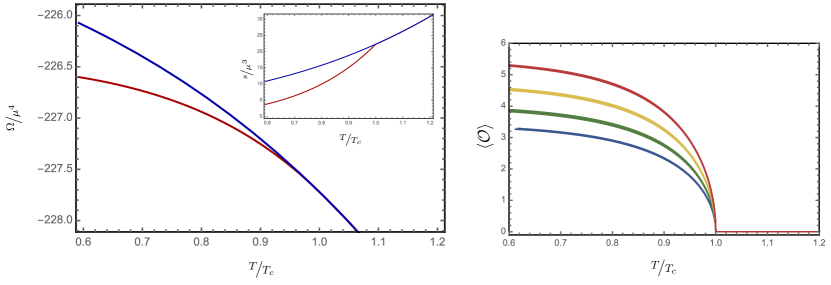
Figure 3: In the left panel, the free energy for solutions with and without a scalar condensate are shown. The blue curve corresponds to solutions without and the red curve with a scalar condensate, respectively. Having a lower value of the grand canonical potential $\Omega$, the solution with a scalar condensate is thermodynamically preferred. The phase transition is second order since the derivative of the entropy is discontinuous at $T=T_{c}$, see inset. In both graphs $\kappa=\nicefrac{{1}}{{\sqrt{2}}}$, $q=5$, $\nicefrac{{p}}{{\mu}}=5.2$, and $\nicefrac{{\lambda}}{{\mu}}=3.3$. In the right panel, the scalar condensate order parameter $\left\langle\mathcal{O}\right\rangle$ is shown for $\nicefrac{{p}}{{\mu}}=4.8$, $5.0$, $5.2$ and $\nicefrac{{\lambda}}{{\mu}}=\color[rgb]{.237736,.340215,.575113}3.0$, $\color[rgb]{.3289465,.5006225,.2625337}3.3$, $\color[rgb]{.8519382,.7451438,.3175208}3.6$, $\color[rgb]{.72987,.239399,.230961}3.9$. The graph shows that the strength of the order parameter is affected much stronger by changes in $\nicefrac{{\lambda}}{{\mu}}$ than by changes in $\nicefrac{{p}}{{\mu}}$: different $\lambda$ leads to each of the four curves shown, while the different $\nicefrac{{p}}{{\mu}}$ lead to nearly the same curves for each value of $\nicefrac{{\lambda}}{{\mu}}$.

The phase transition is second order, since the derivative of the entropy is discontinuous at the transition temperature. The order parameter of the phase transition is the vacuum expectation value $\Braket{\mathcal{O}_{\rho}}$, which is proportional to the boundary mode $\rho_{b}$ of $\rho$. It is plotted as a function of the temperature in Figure 3. The numerical data are consistent with a mean field behavior of the order parameter near the transition temperature, $\Braket{\mathcal{O}_{\rho}}\sim\sqrt{1-T/T_{c}}$. This is expected in the large-$N$ limit, which is intrinsic to our holographic model. For each set of parameters ($\nicefrac{{p}}{{\mu}}$,$\nicefrac{{\lambda}}{{\mu}}$,$q$), the transition temperature $\nicefrac{{T_{c}}}{{\mu}}$ can be determined as the temperature where the order parameter $\Braket{\mathcal{O}_{\rho}}$ vanishes. In this way, the phase diagram of the strongly coupled field theory can be studied numerically. The transition temperature increases as a function of $q$ as is shown in Figure 4.

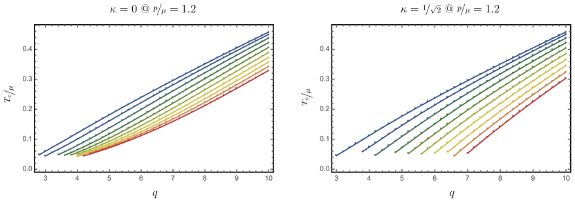
Figure 4: The superfluid phase diagram as a function of the scalar charge $q$ close to the minimal $T_{c}$-value in the phase diagram, i.e. $\nicefrac{{p}}{{\mu}}=1.2$ for $\kappa=0$ (left figure) and $\kappa=\nicefrac{{1}}{{\sqrt{2}}}$ (right figure). As one can see the critical temperature is decreasing with decreasing scalar charge $q$ or increasing backreaction $\sim\nicefrac{{1}}{{q}}$, respectively. This result agrees nicely with the plain s-wave superconductor behavior. Moreover for $\kappa=\nicefrac{{1}}{{\sqrt{2}}}$ and for sufficiently high values of $\nicefrac{{\lambda}}{{\mu}}$ (color coding of the lines represent the following values of $\nicefrac{{\lambda}}{{\mu}}=\color[rgb]{.237736,.340215,.575113}1$, $\color[rgb]{.253651,.344893,.558151}2$, $\color[rgb]{.264425,.423024,.3849}3$, $\color[rgb]{.291469,.47717,.271411}4$, $\color[rgb]{.416394,.555345,.24182}5$, $\color[rgb]{.624866,.673302,.264296}6$, $\color[rgb]{.813033,.766292,.303458}7$, $\color[rgb]{.877875,.731045,.326896}8$, $\color[rgb]{.812807,.518694,.303459}9$, $\color[rgb]{.72987,.239399,.230961}10$) we expect a quantum critical point, where the superconducting phase transition happens at zero temperature. On the other hand, for $\kappa=0$ it seems that the curves are asymptotically approaching zero charge as $T_{c}=0$, and thus there may be no quantum critical point in the $q$ direction.

This can be understood in terms of the effective scalar mass

$$m_{\text{eff}}^{2}=-\frac{q^{2}a^{2}}{U}.$$ (40)

As the scalar charge increases, the effective mass squared becomes more negative which favors the instability. Therefore, the phase transition already appears at higher temperatures. The same behavior was found for translationally invariant holographic s-wave superconductors in Hartnoll2008a . Analyzing the transition temperature as a function of $\nicefrac{{p}}{{\mu}}$ and $\nicefrac{{\lambda}}{{\mu}}$ for different $q$ reveals a more interesting structure as shown for $q=5$ and $q=10$ in Figure 5.

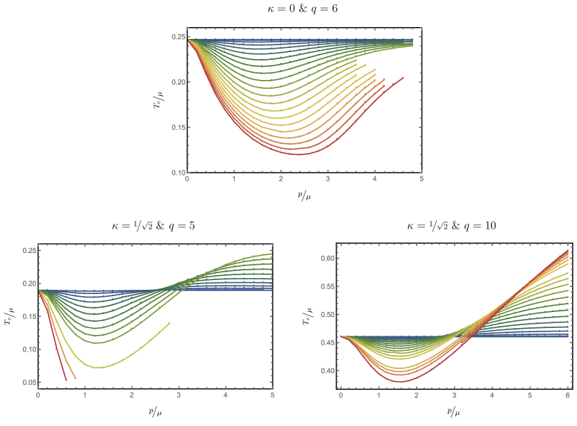
Figure 5: The superfluid phase diagram computed for $\kappa=0$ and scalar charge (or inverse backreaction) $q=6$ in the top panel and for $\kappa=\nicefrac{{1}}{{\sqrt{2}}}$ and $q=5,10$ in the lower panel. Below the respective $T_{c}$-curve, the condensate is non-zero indicating a superfluid phase. Different colored curves correspond to different values of $\nicefrac{{\lambda}}{{\mu}}$ with the following color coding: $\color[rgb]{.237736,.340215,.575113}0$, $\color[rgb]{.244898,.34232,.56748}0.3$, $\color[rgb]{.25206,.344425,.559847}0.6$, $\color[rgb]{.257422,.372239,.497513}0.9$, $\color[rgb]{.26227,.407398,.41955}1.2$, $\color[rgb]{.271186,.43656,.356528}1.5$, $\color[rgb]{.283356,.460926,.305458}1.8$, $\color[rgb]{.310208,.488896,.266972}2.1$, $\color[rgb]{.366424,.524075,.253656}2.4$, $\color[rgb]{.426818,.561243,.242944}2.7$, $\color[rgb]{.52063,.614323,.253058}3$, $\color[rgb]{.614442,.667404,.263172}3.3$, $\color[rgb]{.700133,.710498,.279961}3.6$, $\color[rgb]{.784808,.752343,.297584}3.9$, $\color[rgb]{.832486,.755718,.310489}4.2$, $\color[rgb]{.861664,.739857,.321037}4.5$, $\color[rgb]{.864861,.688575,.322209}4.8$, $\color[rgb]{.835581,.593017,.311662}5.1$, $\color[rgb]{.804513,.490765,.296209}5.4$, $\color[rgb]{.767192,.365082,.263585}5.7$, $\color[rgb]{.72987,.239399,.230961}6$. Note that the case of $\kappa=0$ the minimum of the critical temperature is moving from $\nicefrac{{p}}{{\mu}}=1.8$ at $\nicefrac{{\lambda}}{{\mu}}=1.2$ over $\nicefrac{{p}}{{\mu}}=2$ at $\nicefrac{{\lambda}}{{\mu}}=3$ to $\nicefrac{{p}}{{\mu}}=2.4$ at $\nicefrac{{\lambda}}{{\mu}}=6$, whereas in the case of $\kappa=\nicefrac{{1}}{{\sqrt{2}}}$ the minimum is fixed respect to $\lambda$. However for different values of the scalar charge $q=4,\dotsc,10$ we find a slight increase starting from $\nicefrac{{p}}{{\mu}}=1.2$ and ending at $\nicefrac{{p}}{{\mu}}=1.6$.

In the case of $\kappa=0$ the critical temperature is observed to decrease monotonously as a function of $\nicefrac{{\lambda}}{{\mu}}$. As a function of $\nicefrac{{p}}{{\mu}}$, it first decreases for small $\nicefrac{{p}}{{\mu}}$, then assumes a minimum at $\nicefrac{{p}}{{\mu}}\approx 1.7$, which is slightly shifted towards larger values i.e. $\nicefrac{{p}}{{\mu}}\approx 2.3$ for increasing $\nicefrac{{\lambda}}{{\mu}}\leq 10$, and then returns again to the homogeneous value $T_{c}(\nicefrac{{p}}{{\mu}}=0)$ for large values of $\nicefrac{{p}}{{\mu}}$. This minimum is more pronounced for larger values of $\nicefrac{{\lambda}}{{\mu}}$ which shows that larger values for the source of the helix field indeed increases the effect of the lattice on the system, while the helix momentum dependence has a smaller effect on the transition temperature. This is consistent with the expectation that generally, it is the depth of a lattice of potential valleys which influences the physical behaviour more than the lattice constant or spacing between the individual potential depths. However, for large values of $\nicefrac{{p}}{{\mu}}$ the critical temperature seems to, at least for $\kappa=0$, asymptotically approach the $p=0$ value which might imply that $T_{c}(p\to\infty)\sim T_{c}(p=0)$. In the case of $\kappa=\nicefrac{{1}}{{\sqrt{2}}}$ there is not only a minimal value of $T_{c}$ for $\nicefrac{{p}}{{\mu}}\approx 1.2$ that is robust under changes in $\nicefrac{{\lambda}}{{\mu}}$, but allows for higher values of $T_{c}$ above $\nicefrac{{p}}{{\mu}}\approx 2.6,\dotsc,3$, as displayed in the lower row of Figure 5. Curiously, there the behavior of $\nicefrac{{\lambda}}{{\mu}}$ is inverted, i.e. with increasing $\nicefrac{{\lambda}}{{\mu}}$ the transition temperature, $T_{c}$ is increasing. However, this regime might very well lie far outside of the range of applicability of condensed matter physics since $p>\mu$, suggesting that the “energy stored” in the lattice exceeds the chemical potential. It appears that the critical temperature is unbounded from above unlike in the $\kappa=0$ case where it seems to be bounded by its initial value at $p=0$. Finally, note that in both cases $\kappa=0$ and $\kappa=\nicefrac{{1}}{{\sqrt{2}}}$ the data suggests the existence of a quantum critical point for high values of $\nicefrac{{\lambda}}{{\mu}}\geq 6$ and strong backreaction, i.e. $q\leq 5$, similar to the observations made in Kim:2015dna . One may hence speculate that for a finite range of $q$ there exists a critical value of $\nicefrac{{\lambda}}{{\mu}}$ at zero temperature where the superfluid phase breaks down above a certain $\nicefrac{{p}}{{\mu}}$. We will analyse this possibility further in future work WIP .

3 Optical Conductivity

A main focus of our work is to study the optical conductivity in the $x$-direction, in which translation symmetry is broken for $p\neq 0$. The conductivity is given by the Kubo formula in terms of the retarded Green function of the current operator,

$$\sigma_{x}(\omega)=\lim_{\mathbfit{k}\to 0}\frac{G^{R}_{xx}(\omega,\mathbfit{k})}{\mathrm{i}\omega}.$$ (41)

3.1 Numerical computation of the optical conductivity

We calculate the retarded Green function using the well-established extension of the gauge/gravity correspondence to real-time problems pioneered in Son2002 . Accordingly, the conductivity is determined by linearized perturbations around the background solutions. In a physical picture, the system is slightly perturbed around thermal equilibrium by an external force, the external electric field. The conductivity describes the induced response of the system to these small perturbations. Since the gauge field $A_{\mu}$ corresponds to a conserved current on the field theory side, the electric conductivity is related to the perturbations of $A_{\mu}$. In particular, the fluctuation $\delta A=\mathcal{A}\operatorname{d\mathit{x}}$ governs the conductivity in the $x$-direction. There are certain fields coupling to $\delta A=\mathcal{A}\operatorname{d\mathit{x}}$. To determine them, we write all fields including the metric as a sum of the background solution and a perturbation. Then, the action of (4) is expanded to second order in the perturbations. In this way, a quadratic action $S_{q}$ for the perturbations is obtained, which determines the linearized equations of motion for the perturbations. By analyzing $S_{q}$, all fields coupling to $\delta A=\mathcal{A}\operatorname{d\mathit{x}}$ are determined. The block of coupled perturbations containing $\delta A=\mathcal{A}\operatorname{d\mathit{x}}$ is

$$\delta\left(\operatorname{d\mathit{s}}^{2}\right) =h_{t1}(t,r)\operatorname{d\mathit{t}}\otimes\omega_{1}+h_{23}(t,r)\omega_{2}\otimes\omega_{3}+h_{r1}(t,r)\operatorname{d\mathit{r}}\otimes\omega_{1},$$ (42)

$$\delta A =\mathcal{A}(t,r)\omega_{1},$$

$$\delta B =\mathcal{B}(t,r)\omega_{3}.$$

The remaining perturbations can be set to zero, consistently. The fluctuation fields are chosen to depend on $r$ and $t$ only since the conductivity is evaluated in the limit of vanishing spatial momentum for the Kubo formula (41). The equations of motion for the above perturbations are obtained by varying the quadratic action. After variation, we impose a radial gauge in which $h_{r1}\equiv 0$. In this gauge, the equation for $h_{r1}$ becomes a constraint for the remaining fields. Furthermore, the equations become ordinary differential equations in the radial coordinate after Fourier transforming the time coordinate. In total, we obtain one first order equation (the constraint originating from the $h_{r1}$-equation after choosing radial gauge), and four second order equations for $\mathcal{A},\mathcal{B},h_{t1}$ and $h_{23}$. One of the second order equations can be replaced by the constraint, hence the total differential order of the system is $7=1+2\times 3$. The equation of motion are given in Appendix A.1. The asymptotic expansions of the fluctuation fields, which are necessary for obtaining numerical solutions, are discussed in Appendix B. As usual we implement infalling wave boundary conditions at the thermal horizon $r_{h}$. For $\mathcal{A}$, we find that

$$\mathcal{A}=(r-r_{h})^{\pm\nicefrac{{\mathrm{i}\omega}}{{(4\pi T)}}}\left(A^{h}_{0}+A^{h}_{1}(r-r_{h})+\dotsb\right).$$ (43)

The exponent in the prefactor can assume the values $\pm\nicefrac{{\mathrm{i}\omega}}{{(4\pi T)}}$, which correspond to outgoing and infalling waves, respectively. This can be seen by taking into account the phase factor $\,\mathrm{e}^{-\mathrm{i}\omega t}\,$ of the Fourier transform,

$$\,\mathrm{e}^{-\mathrm{i}\omega t}\,(r-r_{h})^{\pm\nicefrac{{\mathrm{i}\omega}}{{(4\pi T)}}} =\,\mathrm{e}^{\mathrm{i}\omega(\pm\bar{r}-t)}\, \quad\bar{r} =\frac{\ln(r-r_{h})}{(4\pi T)}.$$ with (44)

The infalling solution, i.e. the one with the minus sign, should be used in order to obtain the retarded Green function. The leading behavior of $\mathcal{A}$ near the boundary is found to be

$$\mathcal{A}=A^{b}_{0}+\frac{A^{b}_{2}+A^{b}_{0}\omega^{2}\ln(r)/2}{r^{2}}+\dotsb.$$ (45)

For calculating the conductivity, we have to identify the degrees of freedom coupling to $\mathcal{A}$ by imposing gauge invariance. Even after imposing radial gauge, in which all radial fluctuations vanish, there are still residual gauge transformations left. These consist of the diffeomorphisms and $U(1)$ transformations that do not change the radial gauge $h_{r\mu}\equiv A_{r}\equiv B_{r}\equiv 0$. The residual gauge transformations are worked out in detail in Appendix B.1, following a calculation carried out in Erdmenger2012 in the framework of the holographic $p$-wave system. We find that the relevant physical fields are (i) $\mathcal{A}$, which is already gauge invariant, (ii) $h_{23}$, which is gauge invariant at the boundary $r\to\infty$, and (iii) the linear combination

$$\mathcal{G}=-\mathrm{i}\omega\mathcal{B}+wp\,\mathrm{e}^{-2v_{1}}\,h_{t1}.$$ (46)

The field $h_{t1}$ is not gauge invariant and does therefore not carry physical degrees of freedom. In order to calculate the Green function corresponding to $\mathcal{A}$, we impose the condition that the remaining physical fields, $h_{23}$ and $\mathcal{G}$, have no source term, i.e. that their leading modes for $r\to\infty$ vanish. In this case the renormalized on-shell action for the fluctuations (c.f. Appendix E), expressed in terms of the asymptotic modes of $\mathcal{A}$, is

$$S_{\text{on-shell}}=\int\frac{\operatorname{d\mathit{\omega}}}{2\pi}\operatorname{d^{3}\mathit{\mathbfit{x}}}A^{b}_{0}(-\omega)\left(\frac{A^{b}_{2}(\omega)}{A^{b}_{0}(\omega)}-\frac{\omega^{2}}{4}\right)A^{b}_{0}(\omega).$$ (47)

In this expression, the frequency dependence of the modes is indicated explicitly. The Green function does not follow directly from (47). Following the prescription of Son2002 , one needs to analytically continue the kernel in (47). It follows that

$$G^{R}_{xx}(\omega,0) =2\left(\frac{A^{b}_{2}(\omega)}{A^{b}_{0}(\omega)}-\frac{\omega^{2}}{4}\right),$$ (48)

and, using the Kubo formula (41),

$$\sigma(\omega) =\frac{2A^{b}_{2}(\omega)}{\mathrm{i}\omega A^{b}_{0}(\omega)}+\frac{\mathrm{i}\omega}{2}.$$ (49)

The numerical steps in calculating the conductivity for a given solution to the background equations of motion are described in Appendix D.

3.2 Comparison to the Drude-model and the Two-Fluid-model

For holographic metallic systems in homogeneous translation invariant backgrounds, one finds an ideal metallic behavior related to the conservation of momentum. Thus, strictly speaking the Drude model is not applicable. In the presence of a lattice, momentum is not a conserved quantity and therefore charge carriers can dissipate their momentum within a typical timescale $\tau$ by interactions with the lattice. According to the Drude model (c.f. for example Erdmenger2012a for a review and more details),

$$\sigma(\omega) =\frac{\sigma_{\text{DC}}}{1-\mathrm{i}\omega\tau}, \qquad\operatorname{Re}\sigma(\omega) =\frac{\sigma_{\text{DC}}}{1+\left(\omega\tau\right)^{2}},$$ (50)

the dissipation time scale $\tau$ is inversely proportional to the width of $\operatorname{Re}(\sigma)$ near $\omega=0$, and the Drude peak can be seen as a direct consequence of the translation symmetry breaking lattice. The same reasoning carries over to holographic superconductors. However, in the absence of a momentum dissipating mechanism such as a lattice, the holographic system describes an ideal metal in the normal phase and a mixture of a holographic superconductor and a remaining ideal metal in the condensed phase. In the limit of restored translational symmetry, the Drude peak degenerates into a delta peak at $\omega=0$

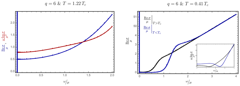
Figure 6: The left panel displays the optical conductivity in the translationally invariant system, i.e. $\nicefrac{{p}}{{\mu}}=0$, or $\nicefrac{{\lambda}}{{\mu}}=0$, respectively. The curves correspond to $q=6$ and $T=1.22\,T_{c}$. The $\nicefrac{{1}}{{\omega}}$ pole indicating an infinite DC conductivity is also present in the normal phase due to momentum conservation. Accordingly, there is no momentum relaxation possible and hence there is no Drude peak at small frequencies. In the superconducting phase, shown in the right panel by the blue lines, the delta peak is enhanced by the superconducting degrees of freedom and the system is a mixture of an ideal metal and a superconductor for finite temperatures $T=0.41\,T_{c}$, as shown in the inset. Comparing the $\omega\to 0$ value of the red line in the left panel $\left.{\omega\operatorname{Im}\sigma}/{\mu^{2}}\right|_{\omega=0}\approx 0.8$ to the black in the inset in the right panel $\left.{\omega\operatorname{Im}\sigma}/{\mu^{2}}\right|_{\omega=0}\approx 0.5$, the “strength” of the ideal metal is reduced but it remains present, whereas the superfluid strength obtains a value of approximately $1.9$.

In our helical setup, translational symmetry can be restored by setting $p=0$ and/or $\lambda=0$. In this case, the helix field $w$ decouples from the system and we obtain the classical holographic model of an s-wave superconductor as introduced in Hartnoll2008 ; Hartnoll2008a . We can understand the translationally invariant case as a limit in which the relaxation time $\tau$ tends to infinity: for $\omega\tau\gg 1$, the Drude conductivity reduces to a $\nicefrac{{1}}{{\omega}}$ pole in $\operatorname{Im}(\sigma)$,

$$\sigma=\mathrm{i}\frac{\sigma_{DC}}{\omega\tau},$$ (51)

which indicates an infinite DC conductivity as explained below (52). Charge carriers which are accelerated by the external field cannot dissipate their momentum and therefore the resulting response is infinite. Consequently, there are two physical mechanisms leading to an infinite DC conductivity in the translationally invariant case. First, there is a contribution for $T<T_{c}$ which is caused by superconductivity. Additionally, there is a contribution due to momentum conservation. It is, therefore, necessary to break translational symmetry in order to determine the superconducting degrees of freedom separately. In Figure 6, we consider the translationally invariant case, and indeed observe the absence of a Drude peak, and the presence of a delta peak $\delta(\omega)$ both in the normal as well as superconducting phases.

Turning on the helical structure $p\neq 0$ and $\lambda\neq 0$, linear momentum is no longer conserved and we find, at last for a weak helix $\nicefrac{{\lambda}}{{\mu}}\ll 1$, a bona fide Drude-model behavior. In Figure 7,

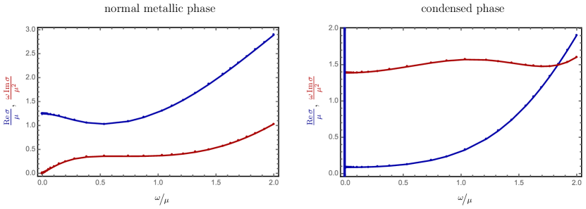
Figure 7: The optical conductivity for $q=0$, $\kappa=0$, $\nicefrac{{p}}{{\mu}}=2.4$,¹³ $\nicefrac{{\lambda}}{{\mu}}=4$ and $T=0.57\,T_{c}$ in the normal phase (left panel) and in the thermodynamically preferred condensed phase (right panel). The real part of the optical conductivity exhibits a broad Drude peak for small frequencies in the normal phase related to the non-conserved linear momentum in the Bianchi type VII helical background. Comparing the normal phase real part of the optical conductivity (blue line) in the left panel with the condensed phase real part of the optical conductivity in the right panel, the developement of a soft gap becomes apparent. The gap scales algebraically with the temperature.

the optical conductivity is shown for $\nicefrac{{p}}{{\mu}}=2.4$, $\nicefrac{{\lambda}}{{\mu}}=1$, and $q=6$ for a certain choice of temperature in the broken phase and for the transition temperature $T_{c}$. For small frequencies, a Drude peak in the real part of the conductivity is observed both in the normal phase at $T_{c}$ and in the superconducting phase. Since we are not strictly at zero temperature, there is a remaining small Drude-like peak after subtraction of the $\nicefrac{{\mathrm{i}}}{{\omega}}$ pole.

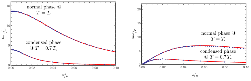
Figure 8: The small-frequency behavior of the optical conductivity in the metallic phase for $q=6$, $\kappa=0$, $\nicefrac{{p}}{{\mu}}=2.4$ and $\nicefrac{{\lambda}}{{\mu}}=1$. The solid lines are fits of the Drude model (50) to the numerically determined optical conductivity. The normal phase solution is given by $\sigma_{DC}=13.6873$ and $\tau=17.4352$. In the superconducting phase the $\nicefrac{{1}}{{\omega}}$ pole has been subtracted from $\operatorname{Im}\sigma$ and there is a remaining “residual” Drude-like peak $\sigma^{\text{reg}}$ as shown in the left panel. As explained in the main text and in Figure 13, this residual contribution to the two-fluid model (54) shows the coexistence of the superconducting phase and a “normal” holographic metal.

Figure 8 shows the small-frequency regime of the optical conductivity $\sigma$ and a corresponding fit to the Drude model. Furthermore, in the condensed phase the imaginary part of the optical conductivity exhibits a $\nicefrac{{1}}{{\omega}}$ pole for $T<T_{c}$ indicating a delta peak in the real part of the optical conductivity related to an infinite DC conductivity, which is a characteristic of superconductivity. This can be inferred from the Kramers-Kronig relation

$$\operatorname{Im}\sigma(\omega)=-\frac{2\omega}{\pi}\mathcal{P}\int_{0}^{\infty}\operatorname{d\mathit{\tilde{\omega}}}\frac{\operatorname{Re}\sigma(\tilde{\omega})}{\tilde{\omega}^{2}-\omega^{2}}.$$ (52)

According to this relation, a $\nicefrac{{1}}{{\omega}}$ pole in the imaginary part of the conductivity is related to a delta function at zero frequency in the real part by

$$\operatorname{Im}\sigma(\omega) =\frac{2\rho_{s}}{\pi}\frac{1}{\omega} \longleftrightarrow \qquad\operatorname{Re}\sigma(\omega) =\rho_{s}\delta(\omega).$$ (53)

This equation defines the superfluid density $\rho_{s}$ as the coefficient of the zero frequency delta function in $\operatorname{Re}(\sigma)$.

As shown in Figure 9, a small Drude peak remains present in the superconducting phase. To describe the system, it is thus necessary to apply the two-fluid model Horowitz2013 , which supplements (53) with the metallic Drude model defined in (50),

$$\operatorname{Re}\sigma(\omega)=\sigma^{\text{reg}}(\omega)+\rho_{s}\delta(\omega)=\left(\chi_{n}(T)\frac{\tau}{1+\omega^{2}\tau^{2}}+\frac{\pi}{2}\chi_{s}(T)\delta(\omega)\right),$$ (54)

where $\chi_{n}(T)$ describes the Drude-like contribution resembling a normal fluid and $\chi_{s}(T)$ the superconducting contribution. In the normal state, we have $\chi_{n}(T>T_{c})=n_{n}$ and $\chi_{s}(T>T_{c})=0$, whereas a pure superconducting state would be described by $\chi_{n}(T<T_{c})=0$ and $\chi_{s}(T<T_{c})=\rho_{s}$. Due to charge conservation $\chi_{n}(T)+\chi_{s}(T)=n$. Moreover, from Figure 9 we observe that the conductivity in the superconducting state develops a gap at low frequencies, i.e. $\operatorname{Re}(\sigma)$ is significantly suppressed. This gap is a characteristic of a superconducting system; it indicates that low-energy charged degrees of freedom have condensed into the delta function at $\omega=0$.

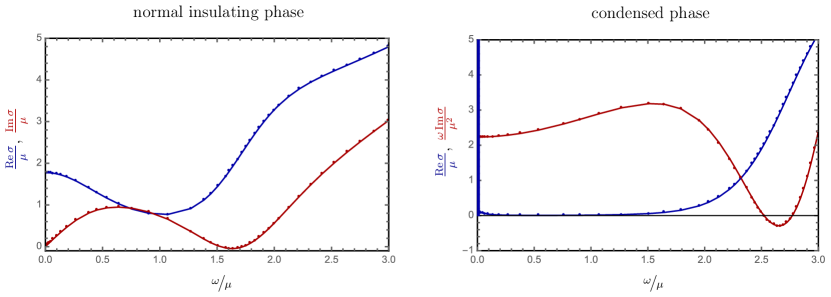
Figure 9: The left plot shows the “insulating” low-temperature phase optical conductivity with vanishing imaginary part as $\omega\rightarrow 0$, which indicates the absence of a delta peak at $\omega=0$ and allows for a proper Drude-like shape. In the right plot the superfluid phase shifts “spectral weight” from the finite frequency part which condensed in a $\omega=0$ delta peak, thus generating the gap in the superconducting state in the region $\nicefrac{{\omega}}{{\mu}}\in[0,1.5]$. Note that this is not a hard gap due to its algebraic temperature scaling on approaching the zero temperature limit and that there is a non-zero contribution coming from a residual Drude-like peak $\sigma^{\text{reg}}$ even at small $T$ in the superfluid phase. As expected from the Kramers-Kronig relations the imaginary part of the optical conductivity displays a $\nicefrac{{1}}{{\omega}}$ pole. Both plots are generated for $\kappa=\nicefrac{{1}}{{\sqrt{2}}}$, $q=6$, $\nicefrac{{p}}{{\mu}}=1.2$, $\nicefrac{{\lambda}}{{\mu}}=1.9$, and $T=0.46\,T_{c}$.

An important issue is whether $\sigma^{\text{reg}}(\omega)$ in (54) vanishes in the limit $T\rightarrow 0$ for frequencies below $\omega_{\mathrm{gap}}$. This would imply $n_{s}=\rho_{s}$ at $T=0$, with $n_{s}$ the thermodynamic density. In general, the following scenarios are possible. One possibility is the presence of a hard gap, in which at low frequencies $0<\omega<\omega_{\mathrm{gap}}$ we have an exponential suppression $\sigma(\omega,T)\sim\exp((\omega-\omega_{\mathrm{gap}})/T)$. On the other hand, for a soft gap there is an algebraic (power law) scaling $\sigma(\omega,T)\sim T^{c_{1}}\omega^{c_{2}}$. In this case, it is much harder to determine numerically whether there exists an additional constant contribution $\sigma_{0}$ to $\sigma(\omega,T)$. As we discuss below, for the model considered in this paper, we find an algebraic scaling. Moreover, by calculating $n_{s}$ and $\rho_{s}$ independently, we find that $n_{s}=\rho_{s}$ for $T\rightarrow 0$ to good numerical accuracy, at least for small $\nicefrac{{p}}{{\mu}}$ and $\nicefrac{{\lambda}}{{\mu}}$. This implies that $\sigma_{0}=0$ in this case, i.e. our system exhibits a soft gap. For translationally invariant holographic s-wave superconductors in $2+1$ dimensions, it is known that, even though highly suppressed, $\operatorname{Re}(\sigma)$ remains nonzero at $T=0$ but finite frequency Horowitz2009 and one finds an algebraic scaling. On the other hand, $p$-wave superconductors are reported to exhibit a hard gap Basu2010 . Also for the helical lattice, by straightforwardly generalising the low frequency analysis in the Appendix of Donos2013c , we conclude that the gap scales algebraically in $\omega$. In addition, we compute $\rho_{s}$ and $n_{s}$ individually at very low temperatures and find indications that they agree to good numerical accuracy. $\rho_{s}$ is read off from the zero frequency pole of the conductivity, while the thermodynamic density $n_{s}$ is obtained from (35). In Figure 10,

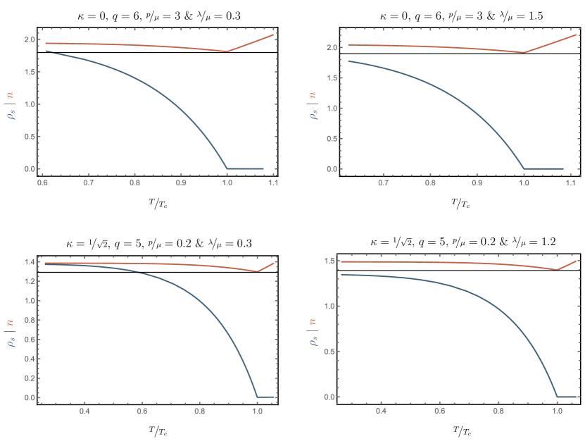
Figure 10: The superfluid density ${\color[rgb]{.257422,.372239,.497513}\rho_{s}}$ and the normalized¹⁷ charge density ${\color[rgb]{.767192,.365082,.263585}n}$ as a function of $\nicefrac{{T}}{{T_{c}}}$. For $T>T_{c}$, the superfluid density vanishes, i.e. the DC conductivity is finite. As $T$ is lowered, the superfluid density ${\color[rgb]{.257422,.372239,.497513}\rho_{s}}$ increases, similar to the order parameter, c.f. Figure 3, and curiously the normalized charge density ${\color[rgb]{.767192,.365082,.263585}n_{s}}$ as well. The gap between ${\color[rgb]{.257422,.372239,.497513}\rho_{s}}$ and ${\color[rgb]{.767192,.365082,.263585}n_{s}}$ is independent of the value of $\nicefrac{{p}}{{\mu}}$, but increases with increasing $\nicefrac{{\lambda}}{{\mu}}$. For small $\nicefrac{{\lambda}}{{\mu}}$, it is suggestive that at $T=0$ the superfluid density and the condensed phase charge density coincide. Thus, the longitudinal response i.e. the plasma frequency in the superconducting phase is sufficient to determine the superfluid strength.

the superfluid density $\rho_{s}$ and the charge density $n_{s}$, c.f. Eq. (34), are plotted as a function of temperature for two sets of parameters. The superfluid density, being a measure for the superconducting degrees of freedom, increases as the temperature is lowered beyond $T_{c}$ and it vanishes for $T>T_{c}$. Of course, in order to finally conclude whether $\rho_{s}$ agrees with $n_{s}$ for $T=0$, as the extrapolation of our data suggests, we need to carefully analyze the zero temperature transport properties, which we are planning to do in future work WIP . Nonetheless, for small $\nicefrac{{p}}{{\mu}}$ and $\nicefrac{{\lambda}}{{\mu}}$ the difference becomes sufficiently small already at finite temperatures about $T\approx 0.6\,T_{c}$. The difference between $\rho_{s}$ and $n_{s}$ at this temperature seems to be independent of the helix pitch, parametrizing the helical lattice constant, but grows with increasing $\nicefrac{{\lambda}}{{\mu}}$. This difference may be accounted for by the residual contribution in the condensed phase for $\omega\to 0$, which is not added to the zero mode delta peak. The optical conductivity of high $T_{c}$ superconductors is known RevModPhys.77.721 to feature residual absorption at very small frequencies, which gives rise to an additional contribution to the imaginary part of $\sigma(\omega,T<T_{c})$. For small helix strengths $\nicefrac{{\lambda}}{{\mu}}\ll 1$, this residual part can be read off by a simple Drude-fit inside the superconducting gap as shown in Figure 8. The spectral weight inside the residual Drude peak accounts exactly for the difference between $\rho_{s}$ and $n_{s}$. On the other hand, for larger helix strengths, i.e. stronger momentum dissipation, the gap cannot be accounted for by the residual spectral weight inside the superconducting gap. We discuss two possible reasons for this behavior in Section 5.2.

3.2.1 Intermediate and High Frequency Regimes

Let us also discuss the behaviour of the optical conductivity in further frequency regimes. First we note that in the intermediary frequency regime $T\ll\omega\ll\mu$, we have not been able to find a scaling law of $|\sigma(\omega)|$. Such a scaling has been observed in the strange metallic phase of the cuprates and interpreted as a consequence of quantum criticality in Marel2003 . While some holographic models Horowitz2012 ; Horowitz2012a ; Vegh2013 ; Horowitz2013 seem to show such a scaling, others Donos2013c do not, and our model seems to be in the latter class. So far a theoretical understanding of the origin of this scaling regime in holographic models is still missing. Concerning the nature of the superconducting gap, there are two more intriguing features: in the case of $\kappa=0$, we find in the vincinity of particular parameter values such as e.g. $\nicefrac{{p}}{{\mu}}=0.8,\nicefrac{{\lambda}}{{\mu}}=3$, plateau-like solutions where the energy scale of the gap as a well as the superfluid density $\rho_{s}$ is drastically reduced, see Figure 11. Curiously, these solutions seem to arise for very low temperatures contrary to the intuition that the gap should grow with decreasing temperature, c.f. the orange line compared to the purple line in Figure 11.

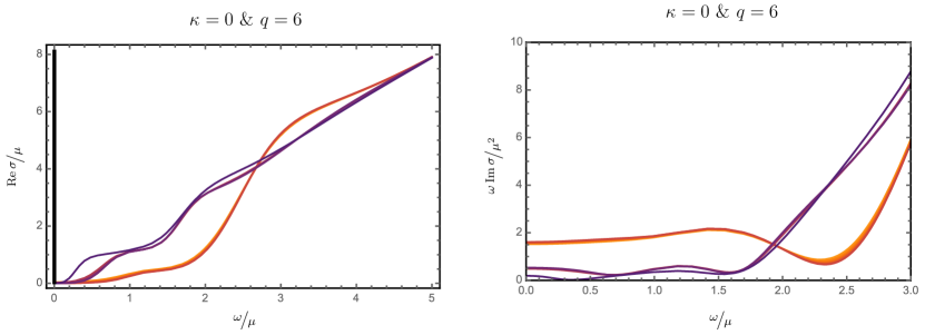
Figure 11: For $\kappa=0$, $\nicefrac{{p}}{{\mu}}=0.8$ and $\nicefrac{{\lambda}}{{\mu}}=3$ we find that the “superconducting gap” is replaced by a plateau-like decay in stark contrast to the right panel of Figure 9, which shows the typical form of the optical conductivity. It is suggestive to compare this result to Figure 16 in Andrade:2014xca where the authors find a similar behavior for low temperatures. Again, the color coding for the temperature is as follows: $\nicefrac{{T}}{{T_{c}}}=\color[rgb]{.991751,.5902,.0983158}0.47$, $\color[rgb]{.985564,.520833,.0747243}0.42$, $\color[rgb]{.979377,.451467,.0511329}0.37$, $\color[rgb]{.92205,.393972,.117026}0.33$, $\color[rgb]{.864723,.336476,.18292}0.28$, $\color[rgb]{.807396,.278981,.248813}0.23$, $\color[rgb]{.705188,.235013,.317923}0.19$, $\color[rgb]{.58054,.197808,.388641}0.14$, $\color[rgb]{.455892,.160603,.459358}0.09$, $\color[rgb]{.335514,.12222,.455853}0.05$. Counter-intuitively, the gap is drastically diminished with decreasing temperature, whereas one would expect the gap to become more pronounced for low temperatures.

A similar behavior has been found in Figure 16 of Andrade:2014xca , although in our case there is no Drude-like peak for higher temperatures close to the transition temperature, which may be attributed to the fact that almost all degrees of freedom have condensed. The same intriguing features are seen for $\kappa=\nicefrac{{1}}{{\sqrt{2}}}$ in the vicinity of particular parameter values such as the ones shown in Figure 12.

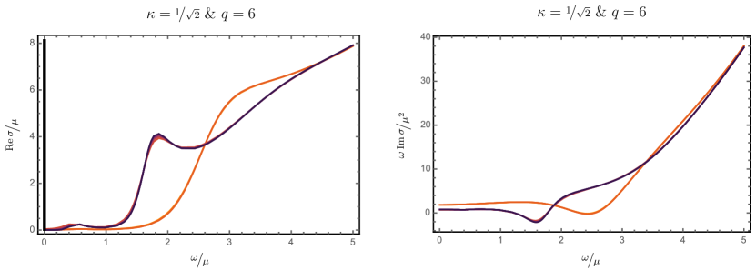
Figure 12: Different shapes of the optical conductivity with additional features compared to Figure 9 for $\nicefrac{{p}}{{\mu}}=0.2$ and $\nicefrac{{\lambda}}{{\mu}}=2$. In the case of $\kappa=\nicefrac{{1}}{{\sqrt{2}}}$ for decreasing temperature the gap seems to get smaller and a new peak arises, interestingly at lower temperatures. The color coding for the temperature is as follows: $\nicefrac{{T}}{{T_{c}}}=\color[rgb]{.991751,.5902,.0983158}0.41$, $\color[rgb]{.984876,.513126,.0721031}0.37$, $\color[rgb]{.966638,.43869,.0657759}0.33$, $\color[rgb]{.902941,.374807,.138991}0.29$, $\color[rgb]{.839244,.310923,.212206}0.25$, $\color[rgb]{.760587,.251548,.286493}0.2$, $\color[rgb]{.622089,.21021,.365068}0.16$, $\color[rgb]{.483591,.168871,.443643}0.12$, $\color[rgb]{.34794,.126747,.472736}0.08$, $\color[rgb]{.223676,.08148,.303902}0.04$. Note that in all cases there is a delta peak in the real part indicating the superfluid phase.

Compared to the more generic result of the optical conductivity shown in Figure 8 and 9, the gap seems to develop a new feature in the intermediary frequency regime that resembles a peak at a non-zero frequency (as shown in Figure 12 at $\nicefrac{{\omega}}{{\mu}}\approx 1.78$) at lower temperatures in the superconducting phase. Again not only the gap is reduced but also the superfluid density; this is evident since the Ferrell-Glover-Tinkham sum rule holds, as proven in the following Section 3.3. These curiosities appear to be due to the contributions of additional resonances below the gap. We plan to investigate these further in future work WIP . Finally, in all cases considered, we find that for large frequencies, $\omega\gg\mu$, the real part of the conductivity is proportional to $\omega$. This behavior is a property of the ultraviolet fixed point of the field theory: since $\sigma$ has energy dimension one, it scales linearly in $\omega$ once the frequency is larger than any other scale of the system.

3.3 Ferrell-Glover-Tinkham Sum Rule

Sum rules are exact identities following from the analytic structure of Green functions. The Ferrell-Glover-Tinkham sum rule PhysRev.109.1398 ; PhysRevLett.2.331q can be expressed as the integral over the real part of the optical conductivity, being a constant regardless of the details of the system,

$$\int_{0}^{\omega_{c}}\operatorname{d\mathit{\omega}}\operatorname{Re}\sigma(\omega)=\text{const.},$$ (55)

Note that the integral includes possible contributions from the lower bound in the form of a delta function at $\omega=0$. Furthermore, while actual condensed matter systems typically become transparent at frequencies larger than the typical electronic energy scales and hence the integral in (55) and (56) converges, in holographic setups it is generically UV divergent due to the UV conformal fixed point behavior of $\operatorname{Re}\sigma(\omega)$. In order to regulate this divergence, we introduced a UV cutoff frequency $\omega_{c}$, to be taken larger than $\max(T,\mu)$. In appropriate formulations of the sum rule such as (57) the UV divergence cancels between the two integrals, and the regulator can be removed. Physically, the sum rule expresses the conservation of charged degrees of freedom, which are measured by the spectral weight, i.e. the area under $\mathrm{Re}(\sigma)$. For example, in the normal phase, Eq. (55) allows to identify the plasma frequency as a measure of the charge density in the system via

$$\frac{\omega_{\text{Pn}}^{2}}{8}=\int_{0}^{\omega_{c}}\operatorname{d\mathit{\omega}}\operatorname{Re}\sigma_{n}(\omega).$$ (56)

In the superfluid phase, this definition excludes the delta function at $\omega=0$. In the case of the superconducting phase transition, where the spectral weight is transferred into the delta function at $\omega=0$, the degrees of freedom can rearrange themselves but they cannot be lost. The Ferrell-Glover-Tinkham sum rule can also be expressed in the form

$$\rho_{s}=\frac{\pi}{2}\lim_{\omega\to 0}\big{[}\omega\operatorname{Im}\sigma_{s}(\omega)\big{]}=\int_{0^{+}}^{\infty}\operatorname{d\mathit{\omega}}\big{[}\operatorname{Re}\sigma_{n}(\omega)-\operatorname{Re}\sigma_{s}(\omega)\big{]}.$$ (57)

Here $\sigma_{n}$ denotes the optical conductivity in the normal phase, i.e. for some $T\geq T_{c}$, $\sigma_{s}$ the conductivity for some temperature below $T_{c}$, and $\rho_{s}$ is the superfluid density at that temperature. The contribution from $\omega=0$ has been separated out explicitly giving rise to the term $\rho_{s}$ determined by $\sigma_{s}$. According to (57), the superfluid density is equal to the missing spectral weight, i.e. the difference in the area under the conductivity curve in the normal and in the superconducting state, c.f. Figure 13.

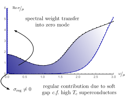
Figure 13: Visualization of the FGT sum rule as explained in the text. The blue area indicates the spectral weight which is transferred into the zero mode. Note the tiny regular contribution which resembles a key property of high-temperature superconductivity and might be responsible for the small possible offset in the computation of $\rho_{s}$, in particular it might account for the missing charge density in the superfluid phase, i.e. the offset between $n_{s}$ and $\rho_{s}$ displayed in Figure 10.

Note that (57) assumes already that the translational symmetry is broken, i.e. a $\delta(\omega)$ contribution or diamagnetic pole in the normal phase is absent. It is convenient to define

$$\mathcal{I}(\omega_{c})=\frac{1}{\rho_{s}}\int_{0^{+}}^{\omega_{c}}\operatorname{d\mathit{\omega}}\left[\operatorname{Re}\sigma_{n}(\omega)-\operatorname{Re}\sigma_{s}(\omega)\right],$$ (58)

in order to apply the sum rule to the numerically calculated conductivities. Here $\omega_{c}$ is a cutoff frequency and the sum rule is satisfied if $\mathcal{I}(\infty)=1$. In Figure 14,

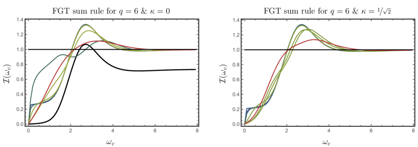
Figure 14: The Ferrell-Glover-Tinkham sum rule holds in the condensed phase for different values of $\nicefrac{{\lambda}}{{\mu}}$ color coded as in Figure 5. The left panel displays the FGT sum rule in the case $\kappa=0$ at the temperature $\nicefrac{{T}}{{\mu}}=0.1$ and $\nicefrac{{\lambda}}{{\mu}}\,(\nicefrac{{p}}{{\mu}})=\color[rgb]{.244898,.34232,.56748}0.3\,(0.4,1)$, $\color[rgb]{.271186,.43656,.356528}1.5\,(0.2,1.4)$, $\color[rgb]{.614442,.667404,.263172}3.3\,(0.2,1)$, $\color[rgb]{.72987,.239399,.230961}6\,(2.4)$, where the numbers in brackets denote the corresponding values of $\nicefrac{{p}}{{\mu}}$. The right panel shows the FGT sum rule for $\kappa=\nicefrac{{1}}{{\sqrt{2}}}$, $\nicefrac{{T}}{{\mu}}=0.05$ and $\nicefrac{{\lambda}}{{\mu}}\,(\nicefrac{{p}}{{\mu}})=\color[rgb]{.244898,.34232,.56748}0.3\,(0.3,1)$, $\color[rgb]{.26227,.407398,.41955}1.2\,(0.2)$, $\color[rgb]{.52063,.614323,.253058}3\,(0.2,1,1.4)$, $\color[rgb]{.72987,.239399,.230961}6\,(1.4)$. The integral $\mathcal{I}(\omega_{c})$ defined in (58) measures the missing spectral weight up to the cutoff $\omega_{c}$ and is normalized so that, if the sum rule is satisfied, $\mathcal{I}(\infty)=1$. As can be seen e.g. from Figure 6 for $\nicefrac{{\omega}}{{\mu}}>8$ the optical conductivity enters the conformal regime, i.e. for $d=3+1$, $\sigma(\omega)\sim\omega$, irrespective of the existence of the “superconducting gap”. In the conformal regime the normal phase and condensed phase optical conductivity becomes identical and thus will not contribute to $\mathcal{I}(\omega)$. Note that the thick black line in the left panel represents the translationally invariant case, $\nicefrac{{p}}{{\mu}}=\nicefrac{{\lambda}}{{\mu}}=0$, and as expected the FGT sum rule fails spectacularly, owing to the coexistence of a ideal metal and a superconductor. Thus, in this case the diamagnetic pole in the imaginary part of the optical conductivity includes not only the missing spectral weight, but also the ideal metal contribution.

$\mathcal{I}(\omega_{c})$ is plotted in the condensed phase for two different temperatures $\nicefrac{{T}}{{\mu}}=0.1,0.05$. As expected, $\mathcal{I}(\omega_{c})$ approaches unity for large enough cutoff frequencies. This confirms the sum rule for the system under consideration and can be seen as a powerful consistency check of the holographic model and of the calculation including the numerics. Physically, it shows that the charged degrees of freedom of the system are conserved. In particular, it uncovers the main obstacle in defining a proper superfluid density in the translational invariant system, since the FGT sum-rule as defined in (58) does not hold due to the coexistence of the normal state ideal metal contributing to the diamagnetic pole, c.f. the black line in Figure 14. Once we turn on our helical structure the “spurious” contribution due to momentum conservation are removed from the diamagnetic pole and the FGT sum rule confirms the conservation of charged degrees of freedom.

3.4 Checking Homes’ and Uemura’s relations

There are two very intriguing relations that were found experimentally, namely Homes’ relation Homes2004 ; Homes2005 ; Dordevic2013 and Uemura’s relation PhysRevLett.62.2317 . The former is given by

$$\rho_{s}(T=0) =C\sigma_{\text{DC}}(T_{c})T_{c}.$$ (59)

whereas the latter reads

$$\rho_{s} =BT_{c}\,,$$ (60)

with $B$ being a proportionality constant of units $mass$ in natural units. Uemura’s relation is found to hold for underdoped cuprates only, while, as demonstrated in Homes2004 ; Homes2005 , Homes’ relation holds for a much broader class of materials. Concerning the units of Homes’ constant, as defined in Section 3.2, $\rho_{s}$ is given in units of $\mu^{2}$ and $\sigma_{\text{DC}}$ as well as $T$ in units of $\mu$. Thus, Homes’ constant given by $\nicefrac{{\rho_{s}}}{{(\sigma_{\text{DC}}T_{c})}}$ is dimensionless in our unit system.

Checking both Homes’ and Uemura’s relations by plotting $\rho_{s}$ against $T_{c}$ and $\sigma_{\text{DC}}T_{c}$, we conclude that Uemura’s relation does not hold in our helical superconducting system. Homes’ linear scaling relation, on the other hand, is clearly visible in Figure 15, where

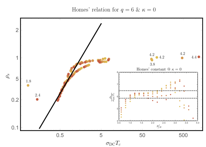
Figure 15: A log-log-plot of the superfluid density $\rho_{s}$ with respect to $\sigma_{\text{DC}}(T_{c})T_{c}$. The color coding for $\nicefrac{{\lambda}}{{\mu}}$ is identical to the phase-diagram plots presented in Figure 5, $\nicefrac{{\lambda}}{{\mu}}=\color[rgb]{.861664,.739857,.321037}4.5$, $\color[rgb]{.864861,.688575,.322209}4.8$, $\color[rgb]{.835581,.593017,.311662}5.1$, $\color[rgb]{.804513,.490765,.296209}5.4$, $\color[rgb]{.767192,.365082,.263585}5.7$ , whereas values of different $\nicefrac{{p}}{{\mu}}$ are not resolved, except for the outliers where the value of $\nicefrac{{p}}{{\mu}}$ is explicitly attached to the point. If Homes’ relation holds, the points should roughly fall on a line with a slope of unity, according to $\log(\rho_{s})=\log C+\log(\sigma_{\text{DC}}T_{c})$ denoted by the black line. The inset shows the value of Homes’ constant $C$ for $\nicefrac{{\lambda}}{{\mu}}=\color[rgb]{.861664,.739857,.321037}4.5$, $\color[rgb]{.864861,.688575,.322209}4.8$, $\color[rgb]{.835581,.593017,.311662}5.1$, $\color[rgb]{.804513,.490765,.296209}5.4$, $\color[rgb]{.767192,.365082,.263585}5.7$. The relation is not expected to hold in the limits of $\nicefrac{{p}}{{\mu}}\to 0$ and $\nicefrac{{p}}{{\mu}}\to\infty$. There the constant approaches zero due to the absence of momentum relaxation and the corresponding divergence of $\sigma_{\text{DC}}$. These data points may be faithfully discarded. Doing so, we see that, in the reasonably applicable range of $\nicefrac{{p}}{{\mu}}\in[1,2]$ Homes’ relation seems to hold within the dashed lines given by $C\approx 6.17\pm 0.31$. This value for the constant is extracted from a least-squares fit represented by the thick black line in the main figure.

we show a log-log plot of $\rho_{s}$ vs $\sigma_{\text{DC}}T_{c}$ for various $(\nicefrac{{\lambda}}{{\mu}},\nicefrac{{p}}{{\mu}})$ with $\kappa=0$. In the range of

$$\frac{\lambda}{\mu} \approx 4.5,\dotsc,6 \quad\frac{p}{\mu} \approx 1,\dotsc,2.$$ and (61)

the relation is linear and extracting Homes’ constant, we find it to be

$$C\approx 6.2\pm 0.3,$$ (62)

Here the uncertainty is not statistical, but refers to the $\pm 5\%$ band bounded by the dashed lines in the inset in Figure 15. Intriguingly, comparing our Homes’ constant with the experimentally found values Homes2004 ; Homes2005 , after correcting for the factor $8$ in our definition of the superfluid density, c.f. footnote 14, the helical system seem to be interpolating between the dirty limit BCS superconductors with $C=\nicefrac{{65}}{{8}}\approx 8.1$ and the in-plane high $T_{c}$ cuprates result $C=\nicefrac{{35}}{{8}}\approx 4.4$ Homes2005 . The error bound may be retrieved from Homes2004 by converting from the dimensionful constant in units of $\nicefrac{{\text{cm}^{-1}}}{{\Omega^{-1}\text{K}}}$ to our dimensionless unit system and yields $C=4.4\pm 0.9$. In fact the value of $C\sim 6.2$ presented in Figure 15, seems to be almost the arithmetic mean of the two experimentally determined values. Additionally, one may compare to the most recent results found for organic superconductors in Dordevic2013 , i.e. $C=(110\pm 60)\,\nicefrac{{\text{cm}^{-1}}}{{\Omega^{-1}\text{K}}}$, again in dimensionful units. Converting to our dimensionless Homes’ constant and including the additional factor of $8$, we find $C=4\pm 2.1$, which is very close to the original result in Homes2004 . Homes’ relation appears to hold for high values of $\nicefrac{{\lambda}}{{\mu}}\gtrsim 4.5$. This is the regime where the Drude peak in the optical conductivity becomes very broad such that the Drude regime, the intermediary frequency regime and the conformal regime are shrinking together, indicating a mixing of IR and UV degrees of freedom. One observation from the finite temperature thermodynamic phase diagram, c.f. Figure 5, is that for such high values of $\nicefrac{{\lambda}}{{\mu}}$ we may hit a quantum critical point at a critical value of $\nicefrac{{p}}{{\mu}}$. On the other hand, Homes’ relation, as shown in the inset of Figure 15, seems to work over a finite range of $\nicefrac{{p}}{{\mu}}$ beyond the possible quantum critical point at $T=0$, which clearly calls for further investigation of the zero temperature system. Alternatively, according to the single scaling argument given in 2005PhRvL..95j7002P Homes’ relation seems to require two competing timescales. In our system the helical lattice introduces an additional timescale for momentum relaxation, controlled by $\nicefrac{{\lambda}}{{\mu}}$, which is very different from the diffusive timescale in the original holographic s-wave superconductor c.f. Erdmenger2012a , at least for small values of $\nicefrac{{\lambda}}{{\mu}}$. It is compelling to speculate that in the large $\nicefrac{{\lambda}}{{\mu}}$ regime, where the applicability of the Drude model may be problematic, these two timescales may become almost identical. Let us stress that for a complete understanding of the aforementioned scaling relations it is imperative to understand the zero temperature phases of the helical system. Nonetheless, the optical conductivity with its broad Drude peak resembles the dirty limit BCS superconductors, where Homes’ relation follows naturally from the missing spectral weight argument: due to the broad peak, we may think of the missing spectral weight area roughly as a square spanned by $\sigma_{\text{DC}}$ and the width of the gap, which is set by the universal gap equation at $T=0$ to be a number times $T_{c}$, see also PhysRevB.73.180504 . We comment on this further in our discussion in section 5.

4 Zero Temperature Solutions and Holographic RG Flows

In order to solve the system at zero temperature and to understand its zero temperature phase diagram and quantum phase transition structure, it is necessary to identify the correct infrared geometries. Classifying all possible IR geometries is in general a complicated task which can only be done by restricting to certain Ansätze and symmetry requirements, but within that class may yield interesting physical insights Charmousis2010 ; Gouteraux:2012yr ; Donos:2014oha . As a possible candidate for such a solution, we now generalize the insulating geometry of Donos2013c to the case of an additional massless charged scalar. We want to emphasize that this insulating geometry is different from the usual gapped AdS-Soliton geometry: Instead of the holographic direction ending at some particular point, the IR of this solution is an anisotropic hyper-scaling violating Lifshitz throat. This anisotropy forces the system to be a smectic material, i.e. an insulator in the direction of the helix (the $x$ direction), and a metal in the other two orthogonal directions. For reasons explained in Section 2.1 we work with a non-vanishing Chern-Simons coupling $\kappa=\nicefrac{{1}}{{\sqrt{2}}}$ (but still $m=m_{\rho}=0$). The solution can be written as a power series in $r^{\nicefrac{{1}}{{3}}}$ with the leading terms being

$$w =w_{0}+w_{1}r^{\nicefrac{{4}}{{3}}}+\dotsb, \rho =\rho_{0}+\rho_{1}r^{\nicefrac{{4}}{{3}}}+\dotsb, a =a_{0}r^{\nicefrac{{5}}{{4}}}+\dotsb,$$ (63)

$$\,\mathrm{e}^{v_{1}} =\,\mathrm{e}^{v_{10}}\,r^{-\nicefrac{{1}}{{3}}}+\dotsb, \,\mathrm{e}^{v_{2}} =\,\mathrm{e}^{v_{20}}\,r^{\nicefrac{{2}}{{3}}}+\dotsb, U =\frac{18}{5}r^{2}+\dotsb$$

$$\,\mathrm{e}^{v_{3}} =\,\mathrm{e}^{v_{30}}\,r^{\nicefrac{{1}}{{3}}}+\dotsb.$$

The coefficients of this expansion can be expressed in terms of the parameters $\rho_{0}$, $v_{20}$ and $v_{30}$. In particular, it follows from the equations of motion that

$$a_{0} =\frac{36\kappa\operatorname{sgn}(p)\,\mathrm{e}^{2v_{20}-2v_{30}}\,}{5\left(6\kappa^{2}+q^{2}\rho_{0}^{2}-4\right)}, w_{0} =\sqrt{3}\,\mathrm{e}^{2v_{30}-v_{20}}\,, \,\mathrm{e}^{v_{10}} =\frac{1}{2}|p|\,\mathrm{e}^{v_{30}-v_{20}}\,,$$ (64)

$$\rho_{1} =-\frac{\kappa^{2}q^{2}\rho_{0}\,\mathrm{e}^{4v_{20}-4v_{30}}\,}{\left(6\kappa^{2}+q^{2}\rho_{0}^{2}-4\right)^{2}}, w_{1} =\frac{\sqrt{3}\left(q^{2}\rho_{0}^{2}-4\right)\,\mathrm{e}^{3v_{20}-2v_{30}}\,}{2\left(6\kappa^{2}+q^{2}\rho_{0}^{2}-4\right)}.$$

This fixed point describes a cohesive IR geometry with a superconducting order parameter turned on. Note that the charged scalar is not subleading or leading compared to the original geometry without it, it rather has the same IR behavior as the helix field $w$. In order to understand whether this fixed point is stable under perturbations, we follow Donos2013c and calculate power law perturbations around (63) by writing

$$w =w_{0}+w_{1}r^{\nicefrac{{4}}{{3}}}(1+c_{w}r^{\delta}), \rho =\rho_{0}+\rho_{1}r^{\nicefrac{{4}}{{3}}}(1+c_{\rho}r^{\delta}), a =a_{0}r^{\nicefrac{{5}}{{4}}}(1+c_{a}r^{\delta}),$$ (65)

$$v_{1} =v_{10}+\log(r^{-\nicefrac{{1}}{{3}}})+c_{1}r^{\delta}, v_{2} =v_{20}+\log(r^{\nicefrac{{2}}{{3}}})+c_{2}r^{\delta}, U =\frac{18}{5}r^{2}(1+c_{U}r^{\delta}),$$

$$v_{3} =v_{30}+\log(r^{\nicefrac{{1}}{{3}}})+c_{3}r^{\delta}.$$

The equations of motion are linearized in the perturbations and solved to leading order in $r$. All scaling exponents and the corresponding eigenvectors for the radial perturbations around (65) are listed in Appendix C.3. In summary, we find that the condensed insulating solution (65) does not show any condensation instabilities in which some of the IR operator dimensions $\delta$ violate the Breitenlohner-Freedman bound by becoming complex. Instead, we find two IR irrelevant deformations, i.e. deformations with explicitly positive exponent, namely the $\delta_{+}$ mode of point 6 and 7 in Appendix C.3,

$$\delta_{1} =\frac{1}{6}\left(\sqrt{145}-5\right), \delta_{2} =\frac{1}{6}\left(\sqrt{185}-5\right).$$ (66)

These perturbations will be useful in generating the RG flows to the UV by shooting numerically from the IR fixed point perturbed with these deformations (c.f. Appendix D for more details). These exponents are the same as the ones found in Donos2013c . As will be explained in detail in Appendix D, these two modes are sufficient to generate the two-parameter family of zero temperature RG flows labeled by the chemical potential $\nicefrac{{\mu}}{{p}}$ and the lattice strength $\nicefrac{{\lambda}}{{p}}$. Besides the above superconducting IR geometry our model admits, at least for large enough Chern-Simons couplings such as our choice $\kappa=\nicefrac{{1}}{{\sqrt{2}}}$, two other IR fixed points: For a vanishing charged scalar, there is a metallic $\text{AdS}_{2}\times\mathds{R}^{3}$ fixed point dominating for larger $p$ Donos2013c , whose geometry including perturbations reads

$$w(r) =c_{w}r^{\delta}, \rho(r) =c_{\rho}r^{\delta}, a(r) =2\sqrt{6}r(1+c_{a}r^{\delta}),$$ (67)

$$v_{1}(r) =v_{10}(1+c_{1}r^{\delta}), \quad v_{2}(r) =v_{20}(1+c_{2}r^{\delta}), \quad U(r) =12{r^{2}}(1+c_{U}r^{\delta}),$$

$$v_{3}(r) =v_{30}(1+c_{3}r^{\delta}).$$

The metallic $\text{AdS}_{2}\times\mathds{R}^{3}$ geometry has several deformation exponents, which are spelled out together with the corresponding eigenvectors in Appendix C.1. Here we focus solely on the condensation instabilities. In particular, there are two modes corresponding to scalar condensation in this $\text{AdS}_{2}$ near horizon geometry, with scaling exponents

$$\delta_{\pm}=\frac{1}{6}\left(-3\pm\sqrt{3(3-2q^{2}+{m_{\rho}}^{2})}\right).$$ (68)

If these exponents become complex, the charged scalar destabilizes the $\text{AdS}_{2}$, and the system presumably flows to the superfluid IR geometry above. Furthermore, there are two exponents connected to the condensation of the helix field,

$$\delta_{\pm}=-\frac{1}{2}\pm\frac{\sqrt{\left(\left(m^{2}+3\right)+p^{2}\,\mathrm{e}^{-2v_{10}}\,-2\sqrt{6}\kappa p\,\mathrm{e}^{v_{10}-2v_{20}}\,\right)}}{2\sqrt{3}}.$$ (69)

Because the lattice is explicitly introduced, the crucial aspect for the physics is now whether the exponent becomes relevant. This happens when $\delta_{+}<0$, see Donos2013c . In that case the system will flow to the insulating geometry. If the exponents become complex, then the $\text{AdS}_{2}$ geometry can spontaneously destabilize to the insulator, but we will not consider this particular case. The insulating geometry of Donos2013c , given by (63) with the charged scalar $\rho$ switched off, is also unstable towards condensation of the charged scalar within the system (4), although in a slightly different way. Analysing the radial perturbations for the case of vanishing scalar mass $m_{\rho}=0$ one finds an additional mode for the charged scalar alone,

$$\delta\rho=c_{0}+c_{1}r^{-\nicefrac{{5}}{{3}}}.$$ (70)

If the charged scalar had a non vanishing mass, its exponents would change from (70) to

$$\delta\rho=c_{0}r^{-\frac{5}{6}\left(1-\sqrt{1+\frac{2}{5}m_{\rho}^{2}}\right)}+c_{1}r^{-\frac{5}{6}\left(1+\sqrt{1+\frac{2}{5}m_{\rho}^{2}}\right)}.$$ (71)

Note that the IR dimension of the charged scalar in the insulating background of Donos2013c is independent of its charge $q$, due to the cohesive nature of the extremal horizon. In the regime

$$-4\leq m_{\rho}^{2}<-\frac{5}{2},$$ (72)

the charged scalar obviously violates the IR Breitenlohner-Freedman bound while preserving the UV Breitenlohner-Freedman bound, and the condensation mechanism will be analogous to the metallic $\text{AdS}_{2}\times\mathds{R}^{3}$ case. On the other hand, for the massless case (70), no condensation instability is found. In this case, condensation can still happen thermodynamically if the condensed zero temperature RG flow obtained from the IR geometry (63) has a lower free energy compared to the uncondensed one (Eq. (63) with $\rho_{0}=0$). We numerically constructed the holographic RG flow geometries up to the asymptotic AdS boundary for both the insulating and superconducting fixed points for a certain range in parameter space, and confirmed that they have lower free energy. For completeness, we collect all the operator dimensions and the corresponding modes for each fixed point in Appendix C.

5 Discussion and Outlook

In this work we analysed the transition to s-wave superconductivity in an anisotropic five-dimensional holographic model with a helical Bianchi $\text{VII}_{0}$ symmmetry. This corresponds to a 3+1 dimensional field theory in the presence of a helical lattice Donos2013c . The advantage of this model is that it allows us to cleanly separate the IR dynamics in the system. This is hard to identify in the simplest holographic superconductors for two reasons: Due to translation invariance there is already in the normal phase a delta peak at zero frequency in the conductivity. In the superconducting phase this mixes with the protected fluctuations of the order parameter. Secondly, most well-known examples of holographic superconductors are accompanied by a remaining gapless Lifshitz sector in the IR that mixes dynamically with the order parameter physics. This is especially so at finite temperature. We improved on the former point by explicitly breaking translation invariance along one of the field theory directions using the above-mentioned Bianchi $\text{VII}_{0}$ helix, and on the latter by using the fact that this model (4) has an anisotropic insulating ground state Donos2013c . We established that this model indeed undergoes a superconducting transition at low temperatures. Studying the optical conductivity we can see that the IR dynamics is more cleanly controlled by order parameter physics. This allowed us to extrapolate to a first holographic example where Homes’ relation holds. Let us discuss the physics of each of these points.

5.1 Phases at Finite and Zero Temperature

The phase diagram of the holographic helical Bianchi $\text{VII}_{0}$ lattice model is quite rich and this is reflected in the ways it approaches superconductivity. For large enough charge $q$ of the scalar order parameter, both the insulating phase at small helix pitch as well as the metallic phase at large helix pitch are unstable towards condensation of the charged scalar. The second order mean field superfluid transition typically happens at a critical temperature $T_{c}(\nicefrac{{\lambda}}{{\mu}},\nicefrac{{p}}{{\mu}})$, but the data in Figure 5 suggests that a quantum phase transition between condensed and uncondensed phases is possible for larger values of $\nicefrac{{\lambda}}{{\mu}}$, similar to the situation in a recently investigated axion-based system Kim:2015dna . The curious aspect is that the critical temperature does not have a monotonic behavior as a function of the helix parameters. Naïvely the presence of a lattice should form an obstacle for s-wave superconductivity. This is true at very small helix parameters. There $T_{c}$ decreases compared to the translationally invariant system. However, for a given value of the amplitude $\lambda$ there is a critical value of the helix pitch $p$ beyond which $T_{c}$ starts to rise again. In the presence of the Chern-Simons coupling, $\kappa=\nicefrac{{1}}{{\sqrt{2}}}$, $T_{c}$ can even increase beyond its isotropic value for very large $\nicefrac{{p}}{{\mu}}$. In the absence of the Chern-Simons coupling, arguably, the tendency to return to its original homogeneous and isotropic value for large $\nicefrac{{p}}{{\mu}}$ can be understood as the effect of the helix diminishing if it rotates too fast around the x-axis: The valleys between the maxima become so narrow that they do not influence the condensation dynamics any longer, and homogeneity is approximately restored. It is an open question whether all observables return to their homogeneous values at large $\nicefrac{{p}}{{\mu}}$, and at which rate. In neither case, however, is the physics behind this behavior of $T_{c}$ very clear. There is a strong indication, on the other hand, that it is correlated with the zero temperature ground state of the system in the normal phase. We did not construct all of these, but one can infer from the finite temperature optical conductivity qualitatively whether the true ground state is insulating or conducting, see Figure 16. These do indicate a second insulating phase occurs at large helix pitch $p$ or equivalently small helix wavelengths. One now sees that there is a rough correlation between high $T_{c}$ with an anisotropic insulating ground state in the normal phase and low $T_{c}$ and a metallic ground state in the normal phase. The correlation is not exact, however. Clearly, an independent analysis from thermodynamic quantities as well as a complete calculation of the zero temperature phase diagram is required to establish this concretely and unambiguously decide the fate of this new insulating phase. The correlation of the behavior of $T_{c}$ with the zero-temperature normal phase ground states indicates that the naïve insight that homogeneity is approximately restored is probably incorrect, as then the system is expected to be in a conducting rather than an insulating phase.

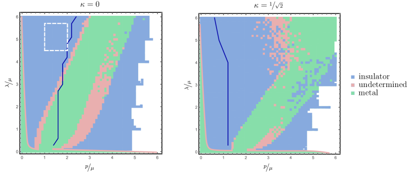
Figure 16: The nature of the zero-temperature ground state from the finite temperature conductivity. The surprise is that for fixed helix amplitude $\lambda$ the system transitions from an insulating to a metallic and then back to an insulating phase. For $\nicefrac{{p}}{{\mu}}\ll 1$ and $\nicefrac{{\lambda}}{{\mu}}\ll 1$, we expect a metallic phase designated by the shaded green area due to the fact that momentum relaxation is removed in the limit where either of these parameters vanishes. This part of the metallic phase could not be distinguished from the insulating phase since we are using very coarse measure to determine the nature of the ground state i.e. a qualitative measure of the conductivity. The thick blue line denotes the location of the minimal critical temperature $T_{c}^{\text{min}}$ extracted from Figure 5. In the case $\kappa=0$, shown in the left panel, this minimum tracks qualitatively the metallic phase inferred from the conductivity, whereas for $\kappa=\nicefrac{{1}}{{\sqrt{2}}}$ the minimal critical temperature $T_{c}^{\text{min}}$ is invariant under changes in $\nicefrac{{p}}{{\mu}}$ and $\nicefrac{{\lambda}}{{\mu}}$. Note that at high values for $\nicefrac{{\lambda}}{{\mu}}$ the critical temperature is very low and thus our numerical code cannot reach $T_{c}^{\text{min}}$ anymore. Homes’ relation holds in the region marked by the white dashed box.

A brief investigation into the possible zero temperature ground states, allowed us to construct an IR geometry dual to the superconducting phase based on the original insulating solution of Donos2013c , c.f. Figure 1. Interestingly, the charged scalar shows the same approach to the IR as the helix field, indicating that they might be able to compete in quantum phase transitions. We analysed the static radial perturbations around these three IR fixed points, in order to understand which RG flows between them are allowed. The situation is summarised in Figure 1: The metallic $\text{AdS}_{2}\times\mathds{R}^{3}$ IR geometry behaves conventionally. It can be unstable towards either the insulating state and/or superconductivity Hartnoll2008 . At the same time the condensed superconducting IR geometry we constructed is nicely stable, indicating that it is the true ground state Donos2013c . The insulating IR geometry is indeed unstable towards superconductivity, but curiously not for the mass of the scalar field considered here. We suspect, however, that in this case the superconducting IR geometry, is still the thermodynamically preferred ground state, i.e. the state of lowest free energy. The insulating but not superconducting geometry of Donos2013c is hence dynamically stable, but thermodynamically unstable. This would indicate that they are separated by a first order transition. We will support this claim by an analysis of the thermodynamics and transport at zero temperature in a forthcoming work WIP .

5.2 Transport

In our system, the linear momentum relaxation introduced by the Bianchi $\text{VII}_{0}$ structure of the geometry allows us to reliably analyse the physics behind the low-frequency transport properties of our system. Our computation reveals that the superconducting system is well described by a two-fluid Drude model at small frequencies in the regime of weak momentum relaxation $\nicefrac{{\lambda}}{{\mu}}\ll 1$, a fact also observed in the models of Andrade:2014xca ; Kim:2015dna . On the other hand, in the regime of stronger momentum relaxation, $\nicefrac{{\lambda}}{{\mu}}\approx 1$, the two-fluid Drude model seems to work less and less well, again similar to Andrade:2014xca ; Kim:2015dna . It is the absence of a diamagnetic pole in the normal phase, that allows us to reliably extract the superfluid density from the $\nicefrac{{1}}{{\omega}}$ pole in the imaginary part of the optical conductivity in the superconducting phase. Naïvely the cohesiveness of the superconducting phases in our system at zero temperature literally forces all charge carriers in the system to condense into the matter fields outside the extremal black hole horizon. Since the $U(1)$ gauge field sourcing the helix itself is not charged under the ‘charge’ $U(1)$ and since the Chern-Simons term in (4) only induces currents but not a charge density for the ‘helix’ $U(1)$, one would expect all the charge density (as carried by the ‘charge’ $U(1)$) in the system at zero temperature to be carried completely by the charged scalar dual to the superconducting order parameter. The charge simply has no other place to go within this system. By comparing the charge density in the superfluid phase at very low temperatures to the superfluid density as extracted from the optical conductivity (c.f. Figure 10), we showed numerically that these indeed become identical for small lattice strengths $\nicefrac{{\lambda}}{{\mu}}\ll 1$. In more detail, we found that when the Drude model is a good approximation to the optical conductivity at small frequencies, i.e. when $\nicefrac{{\lambda}}{{\mu}}\ll 1$, the difference between the charge density at small temperatures and the superfluid density is accounted for by the additional spectral weight residing in a small residual Drude peak at low frequencies. The fact that we are analyzing the system correctly is confirmed by the fact that the Ferrell-Glover-Tinkham sum rule holds (c.f. Figure 14) when crossing the phase transition from the normal to the superconducting phase, i.e. that there is no missing spectral weight in our system. This is to be contrasted with the translationally symmetric case (the black line in the left panel of Figure 14), in which the sum rule fails spectacularly due to the non-accounted spectral weight residing in the $\delta(\omega)$ poles related to momentum conservation in both the normal and superconducting phases. For weak lattice strengths $\nicefrac{{\lambda}}{{\mu}}\ll 1$, the model considered here is therefore in several respects under better control compared to the simple holographic superconductor analyzed e.g. in Erdmenger2012a . A puzzle appears for stronger momentum relaxation $\nicefrac{{\lambda}}{{\mu}}\approx 1$. Now the charge density and superfluid density do not approach each other up to the small temperatures probed in our numerics, and the difference cannot be accounted for any more by a normal fluid Drude component. Even so, the FGT sum rule continues to hold. A possibility is that some of the low frequency spectral weight gets transferred to intermediate frequencies rather than the superfluid pole. Another explanation for the failure could be that our identification of $\rho_{s}$ from the optical conductivity does not match with the superfluid density as calculated from the transverse response via the magnetic/London penetration depth, which is another important cross-check WIP . This deserves further study. Based on the new insulating phase found at high $\nicefrac{{p}}{{\mu}}$, a distinct possibility is that the phase structure of the system is more complicated and interesting for strong lattice potentials at high $\nicefrac{{\lambda}}{{\mu}}$. It is precisely in this novel regime where we can find a region in parameter space in which Homes’ relation is valid to a good accuracy.

5.3 About Homes’ Relation

Homes’ relation Homes2004 ; Homes2005 – the experimental result that for high $T_{c}$ superconductors as well as conventional BCS superconductors, there is a universal relation of the form

$$\rho_{s}(T=0)=C\sigma_{\text{DC}}(T_{c})\cdot T_{c},$$ (73)

with a nearly universal, material independent constant $C$ — would follow naturally from an argument based on the shortest possible time scale in a strongly coupled quantum critical state Marel2003 ; Zaanen2004 , a so-called Planckian dissipator. The basic idea is that in a quantum critical system there is no other scale than the temperature, and hence the relaxation time responsible for the finite electric conductivity in the system must depend on the inverse of the temperature alone, up to numerical factors of $O(1)$. Holography is unique in its ability to model interacting quantum critical systems and the notion of Planckian dissipation is clearly visible in the universal holographic result for the ratio of shear viscosity over entropy density Kovtun:2004de . A holographic foundation for Homes’ relation therefore has the potential to confirm that a similar universal mechanism is at work in superconductivity. In our system, however, the timescale is not the intrinsic timescale associated with the strongly coupled dynamics of the system. Instead it is the external momentum relaxing timescale introduced by the lattice. This is evident from the validity of the Drude response, where $\sigma_{\text{DC}}\sim\tau_{\text{momentum}}$. The relaxation time scale that controls the low-frequency conductivity is thus a function of the lattice strength and helix pitch,

$$\tau_{\text{relax}}=\frac{f(T/\mu,\nicefrac{{\lambda}}{{\mu}},\nicefrac{{p}}{{\mu}},\dots)}{T}.$$ (74)

We have extracted an explicit factor of $T$ such that the function $f$ is dimensionless. A Planckian dissipator would have a mostly constant function $f$ of order $O(1)$ in a CFT. Clearly, for weak momentum relaxation, the relaxation time is typically very large, $\tau T\gg 1$, non-universal and far from a Placnkian dissipator. The breaking of translation invariance and the introduction of an external scale is, however, important in studying Homes’ relation with gauge/gravity duality. As we emphasized, in a translationally invariant system there is already an infinite $\delta$-function contribution to the DC-conductivity. To extract the superfluid density reliably, one needs to resolve this either into a Drude peak behaviour for weak breaking or to something beyond Hartnoll:2007ih ; Hartnoll:2008hs ; Lucas:2015vna . Additionally the system should be in a cohesive phase at low temperatures in order to prevent the existence of additional IR charged degrees of freedom, hidden behind the extremal horizon. It was found in Horowitz2012 ; Horowitz2012a ; Horowitz2013 that a modulated chemical potential is not sufficient to realise Homes’ relation in the simple model considered there. In view of the above, these works probably did not access the regime of strong momentum relaxation that could potentially make Homes’ relation work. For example, in Horowitz2012 ; Horowitz2012a ; Horowitz2013 the two-fluid Drude model works well for all lattices considered, pointing to a regime in which momentum relaxation is weak. Instead, in this work a clearer picture emerges: Due to the cohesive nature of the superconducting ground state, as well as the broken translation invariance in the helix direction, we were able to eliminate, respectively, the additional charged degrees of freedoms in the IR and the zero frequency delta function, hence obtaining a clearer account of the reshuffling of charge density as well as spectral weight during the superfluid transition. As noted already in Erdmenger2012a , to successfully analyse Homes’ relation in a holographic model it is essential to be able to keep track of all charged degrees of freedom at low/zero temperatures. Since our helical lattice model admits an insulator/superconductor transition with a cohesive phase at low temperatures, this setup allows for a fresh look at Homes’ relation, addressing both of these points. Figure 10, which shows the agreement between the superfluid density and the total charge density in the limit $T\rightarrow 0$, illustrates this cleanly, together with our verification that the Ferrell-Glover-Tinkham sum rule holds. The validity of the sum rule is of particular importance, as it can be used to obtain Homes’ relation if the underlying system is a Planckian dissipator Erdmenger2012a . With these results as well as (74), (73) can be reformulated as

$$\frac{n_{s}(T=0)}{n_{n}(T=T_{c})}=C(\nicefrac{{\lambda}}{{\mu}},\nicefrac{{p}}{{\mu}})f(T_{c}/\mu,\nicefrac{{\lambda}}{{\mu}},\nicefrac{{p}}{{\mu}},\dotsc).$$ (75)

with $C$ the coefficient in Homes’ relation. In simple systems, with a single species of charge carriers and a reasonable gap in the superconducting phase, the charge density at zero temperature in the superfluid phase is approximately equal to the charge density at the critical temperature in the normal phase. From (75), Homes’ constant must hence vary inversely with the function $f$ parametrising the momentum relaxation time scale,

$$C\sim 1/f.$$ (76)

In a bona fide Planckian dissipator, $f$ would be a universal constant of $O(1)$, and is in this way seen to explain Homes’ relation. We also investigated the LHS of (75). Figure 17 shows that numerically the charge density in the system does not vary much between $T\ll T_{c}$ and $T_{c}$. Hence in combination with our results from Section 3.2 that the charge density and superfluid density are approximately equal at low $T$, also the ratio of charge densities in (75) is seen to be close to unity. This is so in the weak momentum relaxation regime where $\nicefrac{{\lambda}}{{\mu}}\ll 1$, but also for rather large $\nicefrac{{\lambda}}{{\mu}}$, i.e. strong momentum relaxation in which the Drude model is not readily applicable. in this case Homes’ relation may hold. As we found in Section 3.4, explicitly computing the functional relation between $\rho_{s}$ and $\sigma_{\text{DC}}(T_{c})T_{c}$ we indeed find that in our holographic superconductor in a helical lattice Homes’ relation holds with coefficient

$$C\approx 6.2\pm 0.3$$ (77)

in the range of parameters

$$\frac{\lambda}{\mu} \approx 4.5,\dotsc,6, \quad\frac{p}{\mu} \approx 1,\dotsc,2, \quad\kappa =0.$$ and for (78)

It can, however, not be explained as a consequence of the simple ratio of charge densities at $T_{c}$ and $T=0$. This is also the regime where a difference between $\rho_{s}$ and $n_{s}$ opens (c.f. Figure 10), and the simple relation between (75) and (73) breaks down. As we now argue, the fact that Homes’ relation does hold in the parameter range given above may on the contrary be due to a strong deviation from the simple Planckian dissipation behavior. We may parametrize the difference between $\rho_{s}$ and $n_{s}$ as

$$\rho_{s}(T=0)=n_{s}(T=0)+\delta\rho_{s}(T=0).$$ (79)

Furthermore, let us assume the DC conductivity is still roughly proportional to the charge density times a relaxation time,

$$\sigma_{DC}=n_{n}\tau.$$ (80)

Substituting Homes’ relation on the LHS of (79) together with (80), and using that the ratio (75) is close to unity, we arrive at

$$Cf(T_{c},\nicefrac{{\lambda}}{{\mu}},\nicefrac{{p}}{{\mu}},\dotsc)=1+\frac{\delta\rho_{s}(T=0,\nicefrac{{\lambda}}{{\mu}},\nicefrac{{p}}{{\mu}},\dotsc)}{n_{n}(T_{c},\nicefrac{{\lambda}}{{\mu}},\nicefrac{{p}}{{\mu}},\dotsc)}.$$ (81)

Then, for Homes’ relation (73) to be valid and $C$ to be a univeral constant of $O(1)$, we see that the gap $\delta\rho_{s}$ and the function $f$ cannot vary independently from each other, but must conspire. As $\delta\rho_{s}$ varies with the parameters, $f$ cannot be constant, and hence the system is not a Planckian dissipator. A more detailed investagation of the function $f$ directly as well as other relaxational scales is hence of great interest, as well as how the gap $\delta\rho_{s}$ behaves in the regime of strong(er) scattering. Since this is no longer Drude physics, it requires a more detailed response analysis to extract these. We do note that the regime of $\nicefrac{{p}}{{\mu}}$ and $\nicefrac{{\lambda}}{{\mu}}$ where we find Homes’ relation to hold is near the apparent insulator-metallic quantum phase transition in the normal phase, see Figure 16. It will hence be very interesting to investigate in more detail the behavior of the above quantities in the zero temperature ground states WIP . To conclude, we would like to emphasize that in our model we have found an example of the validity of Homes’ relation in a holographic model with strong momentum relaxation. This is similar to the experimental result Homes2004 ; Homes2005 in which the c-axis high $T_{c}$ cuprates as well as the dirty limit BCS superconductors, both materials with strong scattering and momentum relaxation, follow the same Homes’ relation. As explained above, in the strong momentum relaxation regime there is a nontrivial difference between $\rho_{s}$ and $n_{s}$ at low temperatures, whose origin needs to be investigated in more detail WIP . An important consistency check will be to compute the superfluid strength not from the longitudinal response, i.e. the plasma frequency and the Drude weight, but from the transverse response by determining the magnetic/London penetration depth. This requires to solve for the transverse propagator by finding a solution at small but non-zero momentum. Indeed, an analysis of the dynamical conductivity $\sigma_{xx}(\omega,\vec{k})$ and possible finite momentum instabilities WIP2 will allow us to determine the spectrum of quasi-particle excitations, and also whether the superconducting phase (63) is really the thermodynamically preferred ground state in our system. There is another interesting aspect to consider, that is the case of spontaneously generated helical ground states. Similar to the case of spontaneous generated charge density waves Nakamura:2009tf ; Donos:2011bh ; Withers:2013loa ; Ling:2014saa this might even dynamically fix the preferred helix pitch $p$, leaving fewer free UV parameters. If Homes’ relation hold for all such spontaneous helix models, then one would have a more satisfying reason to explain its universality. At this stage, all these results are still preliminary and for $\kappa=0$ only, and we plan to analyze the question under which exact conditions Homes’ relation holds and related questions, in a future work WIP .

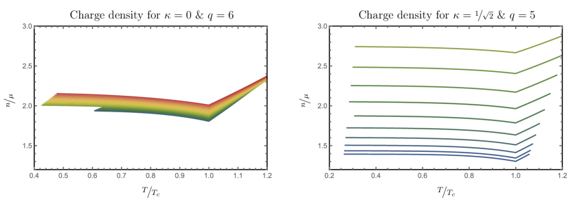
Figure 17: The charge density as a function of $\nicefrac{{T}}{{T_{c}}}$ for $\nicefrac{{p}}{{\mu}}=0.4$ and for various values of $\nicefrac{{\lambda}}{{\mu}}$, using the same color coding as in Figure 5: $\color[rgb]{.244898,.34232,.56748}0.3$, $\color[rgb]{.25206,.344425,.559847}0.6$, $\color[rgb]{.257422,.372239,.497513}0.9$, $\color[rgb]{.26227,.407398,.41955}1.2$, $\color[rgb]{.271186,.43656,.356528}1.5$, $\color[rgb]{.283356,.460926,.305458}1.8$, $\color[rgb]{.310208,.488896,.266972}2.1$, $\color[rgb]{.366424,.524075,.253656}2.4$, $\color[rgb]{.426818,.561243,.242944}2.7$, $\color[rgb]{.52063,.614323,.253058}3$, $\color[rgb]{.614442,.667404,.263172}3.3$, $\color[rgb]{.700133,.710498,.279961}3.6$, $\color[rgb]{.784808,.752343,.297584}3.9$, $\color[rgb]{.832486,.755718,.310489}4.2$, $\color[rgb]{.861664,.739857,.321037}4.5$, $\color[rgb]{.864861,.688575,.322209}4.8$, $\color[rgb]{.835581,.593017,.311662}5.1$, $\color[rgb]{.804513,.490765,.296209}5.4$, $\color[rgb]{.767192,.365082,.263585}5.7$, $\color[rgb]{.72987,.239399,.230961}6$ in the case of $\kappa=0$ (left panel) and $\color[rgb]{.244898,.34232,.56748}0.3$, $\color[rgb]{.25206,.344425,.559847}0.6$, $\color[rgb]{.257422,.372239,.497513}0.9$, $\color[rgb]{.26227,.407398,.41955}1.2$, $\color[rgb]{.271186,.43656,.356528}1.5$, $\color[rgb]{.283356,.460926,.305458}1.8$, $\color[rgb]{.310208,.488896,.266972}2.1$, $\color[rgb]{.366424,.524075,.253656}2.4$, $\color[rgb]{.426818,.561243,.242944}2.7$, $\color[rgb]{.52063,.614323,.253058}3$ for $\kappa=\nicefrac{{1}}{{\sqrt{2}}}$ (right panel). Curiously, the charge density at the phase transition seems to be minimal and hence $n_{s}(T<T_{c})>n_{n}(T_{c})$. Note that this is more prominent at vanishing Chern-Simons coupling $\kappa$. The decrease of the charge density in the normal phase can be attributed to the effects of the insulating phase, i.e. there are less charged degrees of freedom available for lower temperature. However, in the superconducting phase the system turns completely into the condensed state which is growing with lower temperatures. Therefore, the superconducting degrees of freedom are increasing for lower temperatures and may be drawn from the metallic directions, due to partial restoration of the isotropy.

Appendix A Equations of Motion for S-Wave Superconductors on a Helical Lattice

The equations of motion for the metric fields $U,v_{1},v_{2},v_{3}$, the Maxwell fields $A$ and $B$, and the scalar field $\rho$ following from the action (4) are

$$0={} a^{\prime\prime}+a^{\prime}\left(v_{1}^{\prime}+v_{2}^{\prime}+v_{3}^{\prime}\right)-\frac{2aq^{2}\rho^{2}}{U}+\kappa p\,\mathrm{e}^{-v_{1}-v_{2}-v_{3}}\,ww^{\prime},$$ (82)

$$0={} w^{\prime\prime}+w^{\prime}\left(\frac{U^{\prime}}{U}+v_{1}^{\prime}-v_{2}^{\prime}+v_{3}^{\prime}\right)+\frac{w}{U}\left(\kappa p\,\mathrm{e}^{-v_{1}+v_{2}-v_{3}}\,a^{\prime}-m^{2}-p^{2}\,\mathrm{e}^{-2\left(v_{1}-v_{2}+v_{3}\right)}\,\right),$$

$$0={} 2\rho^{2}\left(m_{\rho}^{2}-\frac{a^{2}q^{2}}{U}\right)+a^{\prime 2}+w^{2}\left(m^{2}\,\mathrm{e}^{-2v_{2}}\,+p^{2}\,\mathrm{e}^{-2\left(v_{1}+v_{3}\right)}\,\right)+4p^{2}\,\mathrm{e}^{-2v_{1}}\,\sinh^{2}\left(v_{2}-v_{3}\right)$$

$$+2U\left(v_{1}^{\prime}+v_{2}^{\prime}+v_{3}^{\prime}\right)-U\left(2\rho^{\prime 2}+\,\mathrm{e}^{-2v_{2}}\,w^{\prime 2}-4v_{1}^{\prime}v_{2}^{\prime}-4v_{1}^{\prime}v_{3}^{\prime}-4v_{2}^{\prime}v_{3}^{\prime}\right)-24,$$

$$0={} 2\rho^{2}\left(\frac{m_{\rho}^{2}}{U}-\frac{a^{2}q^{2}}{U^{2}}\right)-\frac{a^{\prime 2}}{U}+\frac{w^{2}}{U}\left(m^{2}\,\mathrm{e}^{-2v_{2}}\,-p^{2}\,\mathrm{e}^{-2\left(v_{1}+v_{3}\right)}\,\right)$$

$$+\frac{p^{2}}{U}\left(-2\,\mathrm{e}^{-2v_{1}}\,+3\,\mathrm{e}^{-2\left(v_{1}+v_{2}-v_{3}\right)}\,-\,\mathrm{e}^{-2\left(v_{1}-v_{2}+v_{3}\right)}\,\right)+2\rho^{\prime 2}+\frac{2U^{\prime\prime}}{U}$$

$$+4\left(\frac{U^{\prime}}{U}\left(v_{1}^{\prime}+v_{2}^{\prime}\right)+v_{1}^{\prime 2}+v_{2}^{\prime}v_{1}^{\prime}+v_{2}^{\prime 2}\right)-\frac{24}{U}+\,\mathrm{e}^{-2v_{2}}\,w^{\prime 2}+4\left(v_{1}^{\prime\prime}+v_{2}^{\prime\prime}\right),$$

$$0={} \frac{2w^{2}}{U}\left(p^{2}\,\mathrm{e}^{-2\left(v_{1}+v_{3}\right)}\,-m^{2}\,\mathrm{e}^{-2v_{2}}\,\right)+\frac{4p^{2}}{U}\left(\,\mathrm{e}^{-2\left(v_{1}-v_{2}+v_{3}\right)}\,-\,\mathrm{e}^{-2\left(v_{1}+v_{2}-v_{3}\right)}\,\right)$$

$$+\frac{4U^{\prime}}{U}\left(v_{3}^{\prime}-v_{2}^{\prime}\right)-2\,\mathrm{e}^{-2v_{2}}\,w^{\prime 2}+4\left(-v_{2}^{\prime 2}-v_{1}^{\prime}v_{2}^{\prime}+v_{3}^{\prime 2}+v_{1}^{\prime}v_{3}^{\prime}\right)+4\left(v_{3}^{\prime\prime}-v_{2}^{\prime\prime}\right),$$

$$0={} \frac{p^{2}}{U}\left(\,\mathrm{e}^{-2v_{1}}\,-\,\mathrm{e}^{-2\left(v_{1}+v_{2}-v_{3}\right)}\,\right)+\frac{U^{\prime}}{U}\left(v_{3}^{\prime}-v_{1}^{\prime}\right)-v_{1}^{\prime 2}+v_{3}^{\prime 2}-v_{1}^{\prime}v_{2}^{\prime}+v_{2}^{\prime}v_{3}^{\prime}-v_{1}^{\prime\prime}+v_{3}^{\prime\prime},$$

$$0={} \rho^{\prime\prime}+\rho^{\prime}\left(\frac{U^{\prime}}{U}+v_{1}^{\prime}+v_{2}^{\prime}+v_{3}^{\prime}\right)+\rho\left(\frac{a^{2}q^{2}}{U^{2}}-\frac{m_{\rho}^{2}}{U}\right).$$

The third equation is first order and originates from the $rr$-component of the Einstein equations. There is another second order equation

$$\frac{a^{2}q^{2}\rho^{2}}{U^{2}}+\rho^{\prime 2}+\frac{1}{2}\,\mathrm{e}^{-2v_{2}}\,w^{\prime 2}+v_{1}^{\prime 2}+v_{2}^{\prime 2}+v_{3}^{\prime 2}+v_{1}^{\prime\prime}+v_{2}^{\prime\prime}+v_{3}^{\prime\prime}=0,$$ (83)

which follows from the above equations. Therefore, the first order equation is a constraint. In the above equations, we have made use of the $U(1)$ symmetry associated with $A_{\mu}$ to choose $\rho$ real.

A.1 Linear Response for S-Wave Superconductors on a Helical Lattice

We consider linearized fluctuations around the background solution. Therefore, we write

$$g_{\mu\nu} =g^{b}_{\mu\nu}+h_{\mu\nu}, \qquad\qquad A_{\mu} =A^{b}_{\mu}+A^{f}_{\mu},$$ (84)

$$B_{\mu} =B^{b}_{\mu}+B^{f}_{\mu}, \rho =\rho^{b}+\rho^{f},$$

where the fields with a superscript ‘$b$’ denote the background solutions, $h$ denotes the metric fluctuation, and fields with a superscript ‘$f$’ denote the matter fluctuations. The metric and the vector fields are expanded in the basis $(\operatorname{d\mathit{t}},\operatorname{d\mathit{r}},\omega_{1},\omega_{2},\omega_{3})$. The background fields are $r$-dependent only and are written in the Ansatz of Eqs. (15), (11) and (12). The fluctuation fields are chosen to depend on $r$ and $t$ because the retarded Green function leading to the conductivity is evaluated at zero spatial momentum, Eq. (41). Expanding the action of Eq. (4) to second order in the fluctuations, we obtain an action $S_{q}$ that determines the linearized equations of motion. The term linear in the fluctuations vanishes upon use of the equations of motions for the background fields. Analyzing the action $S_{q}$, we can determine which fields couple to each other. The result of this analysis is summarized in Table 1 on page 1. The block of fluctuations which contains $A^{f}_{1}$ and decouples from all other fluctuations is

$$\left(\mathcal{A}\equiv A^{f}_{1},\mathcal{B}\equiv B^{f}_{3},h_{t1},h_{23},h_{r1}\right).$$ (85)

It is more convenient to work with the fields

$$\mathcal{E} =(g^{b})^{11}\;h_{t1}=\,\mathrm{e}^{-2v_{1}}\,h_{t1},$$ (86)

$$\mathcal{F} =(g^{b})^{22}\;h_{23}=\,\mathrm{e}^{-2v_{2}}\,h_{23},$$ (87)

instead of $h_{t1}$ and $h_{23}$. The reason is that $\mathcal{E}$ and $\mathcal{F}$ have a finite limit for $r\to\infty$, whereas $h_{t1}$ and $h_{23}$ are proportional to $r^{2}$ for large values of $r$. The equations of motion for the fluctuations are obtained by varying the action $S_{q}$. After variation, we can set $h_{r1}=0$ choosing radial gauge in which all radial field components vanish. Carrying out a Fourier transform of the time coordinate, i.e. choosing a harmonic time dependence $\,\mathrm{e}^{-\mathrm{i}\omega t}\,$, we obtain the following linearly coupled ordinary differential equations in $r$ for the fluctuation fields $\mathcal{A}$, $\mathcal{B}$, $\mathcal{E}$, and $\mathcal{F}$:

$$0={} \mathcal{A}^{\prime\prime}+\mathcal{A}^{\prime}\left(\frac{U^{\prime}}{U}-v_{1}^{\prime}+v_{2}^{\prime}+v_{3}^{\prime}\right)+\mathcal{A}\left(\frac{\omega^{2}}{U^{2}}-\frac{2q^{2}\rho^{2}}{U}\right)$$ (88)

$$+\frac{\mathrm{i}\mathcal{B}\kappa\,\mathrm{e}^{v_{1}-v_{2}-v_{3}}\,\omega w^{\prime}}{U}-\frac{\kappa p\mathcal{E}\,\mathrm{e}^{v_{1}-v_{2}-v_{3}}\,ww^{\prime}}{U}+\frac{\,\mathrm{e}^{2v_{1}}\,a^{\prime}\mathcal{E}^{\prime}}{U},$$

$$={} \mathcal{B}^{\prime\prime}+\mathcal{B}^{\prime}\left(\frac{U^{\prime}}{U}+v_{1}^{\prime}+v_{2}^{\prime}-v_{3}^{\prime}\right)+\mathcal{B}\left(\frac{\kappa pa^{\prime}}{U}\,\mathrm{e}^{v_{3}-v_{1}-v_{2}}\,-\frac{m^{2}}{U}-\frac{p^{2}}{U}\,\mathrm{e}^{2\left(v_{3}-v_{1}-v_{2}\right)}\,+\frac{\omega^{2}}{U^{2}}\right)$$

$$+\frac{\kappa}{U}\left(\mathcal{F}p\,\mathrm{e}^{-v_{1}+v_{2}-v_{3}}\,wa^{\prime}-\mathrm{i}\mathcal{A}\,\mathrm{e}^{-v_{1}-v_{2}+v_{3}}\,\omega w^{\prime}\right)-\frac{\mathcal{F}p^{2}w}{U}\left(\,\mathrm{e}^{-2v_{1}}\,+\,\mathrm{e}^{-2\left(v_{1}-v_{2}+v_{3}\right)}\,\right)$$

$$+2\mathcal{F}w^{\prime}\left(v_{3}^{\prime}-v_{2}^{\prime}\right)+\frac{\mathrm{i}p\mathcal{E}w\omega}{U^{2}}-\mathcal{F}^{\prime}w^{\prime}$$

$$0={} \mathcal{F}^{\prime\prime}+\mathcal{F}^{\prime}\left(\frac{U^{\prime}}{U}+v_{1}^{\prime}+3v_{2}^{\prime}-v_{3}^{\prime}\right)-\frac{\mathrm{i}p\mathcal{E}\,\mathrm{e}^{2v_{3}-2v_{2}}\,\omega}{U^{2}}+\frac{\mathrm{i}p\mathcal{E}\omega}{U^{2}}+\,\mathrm{e}^{-2v_{2}}\,\mathcal{B}^{\prime}w^{\prime}$$

$$+\mathcal{F}\bigg{[}\frac{\omega^{2}}{U^{2}}-\,\mathrm{e}^{-2v_{2}}\,w^{\prime 2}-\frac{m^{2}\,\mathrm{e}^{-2v_{2}}\,w^{2}}{U}-\frac{2p^{2}}{U}\left(\,\mathrm{e}^{-2v_{1}}\,+\,\mathrm{e}^{-2\left(v_{1}+v_{2}-v_{3}\right)}\,\right)\bigg{]}$$

$$+\frac{\mathcal{B}m^{2}\,\mathrm{e}^{-2v_{2}}\,w}{U}-\frac{\mathcal{B}p^{2}\,\mathrm{e}^{-2\left(v_{1}+v_{2}\right)}\,w}{U}$$

$$0={} \mathcal{E}^{\prime}+\mathcal{A}\,\mathrm{e}^{-2v_{1}}\,a^{\prime}+\frac{\mathrm{i}\mathcal{F}pU}{\omega}\left(\,\mathrm{e}^{-2\left(v_{1}+v_{3}\right)}\,ww^{\prime}+2\,\mathrm{e}^{-2v_{1}}\,v_{2}^{\prime}-2\,\mathrm{e}^{-2v_{1}}\,v_{3}^{\prime}\right)$$

$$+\frac{\mathrm{i}pU}{\omega}\left(\mathcal{B}\,\mathrm{e}^{-2\left(v_{1}+v_{2}\right)}\,w^{\prime}-\,\mathrm{e}^{-2\left(v_{1}+v_{3}\right)}\,w\mathcal{B}^{\prime}\right)+\frac{\mathrm{i}pU\mathcal{F}^{\prime}}{\omega}\left(\,\mathrm{e}^{-2v_{1}}\,-\,\mathrm{e}^{-2\left(v_{1}-v_{2}+v_{3}\right)}\,\right).$$

The first three equations are second order. The last one – the constraint – is first order and originates from the metric mode $h_{r1}$ after choosing radial gauge. There is a forth second order equation,

$$0={} \mathcal{E}^{\prime\prime}+\mathcal{E}^{\prime}\left(3v_{1}^{\prime}+v_{2}^{\prime}+v_{3}^{\prime}\right)+\,\mathrm{e}^{-2v_{1}}\,a^{\prime}\mathcal{A}^{\prime}+\frac{2a\mathcal{A}q^{2}\rho^{2}\,\mathrm{e}^{-2v_{1}}\,}{U}$$

$$+\mathcal{E}\frac{p^{2}}{U}\left(2\,\mathrm{e}^{-2v_{1}}\,-\,\mathrm{e}^{-2\left(v_{1}+v_{3}\right)}\,w^{2}-\,\mathrm{e}^{-2\left(v_{1}+v_{2}-v_{3}\right)}\,-\,\mathrm{e}^{-2\left(v_{1}-v_{2}+v_{3}\right)}\,\right)$$

$$+\mathrm{i}\frac{p\omega}{U}\left(\mathcal{B}\,\mathrm{e}^{-2\left(v_{1}+v_{3}\right)}\,w-\mathcal{F}\,\mathrm{e}^{-2v_{1}}\,+\mathcal{F}\,\mathrm{e}^{-2\left(v_{1}-v_{2}+v_{3}\right)}\,\right),$$ (89)

which follows from the above equations and the equations of motion for the background fields. The background equations of motion have been used to eliminate second order derivatives of background fields in the above equations.

$h_{tt}$

$h_{rr}$

$h_{11}$

$h_{22}$

$h_{33}$

$h_{tr}$

${\color[rgb]{.7,0,0}h_{t1}}$

$h_{t2}$

$h_{t3}$

${\color[rgb]{.7,0,0}h_{r1}}$

$h_{r2}$

$h_{r3}$

$h_{12}$

$h_{13}$

${\color[rgb]{.7,0,0}h_{23}}$

$A^{f}_{t}$

$A^{f}_{r}$

${\color[rgb]{.7,0,0}A^{f}_{1}}$

$A^{f}_{2}$

$A^{f}_{3}$

$B^{f}_{t}$

$B^{f}_{r}$

$B^{f}_{1}$

$B^{f}_{2}$

${\color[rgb]{.7,0,0}B^{f}_{3}}$

$\rho^{f}$

$\left(\rho^{f}\right)^{\ast}$

$h_{tt}$

$\bullet$

$\bullet$

$\bullet$

$\bullet$

$\bullet$

$\bullet$

$\bullet$

$\bullet$

$\bullet$

$\bullet$

$\bullet$

$h_{rr}$

$\bullet$

$\bullet$

$\bullet$

$\bullet$

$\bullet$

$\bullet$

$\bullet$

$\bullet$

$\bullet$

$\bullet$

$h_{11}$

$\bullet$

$\bullet$

$\bullet$

$\bullet$

$\bullet$

$\bullet$

$\bullet$

$\bullet$

$\bullet$

$h_{22}$

$\bullet$

$\bullet$

$\bullet$

$\bullet$

$\bullet$

$\bullet$

$\bullet$

$\bullet$

$h_{33}$

$\bullet$

$\bullet$

$\bullet$

$\bullet$

$\bullet$

$\bullet$

$\bullet$

$h_{tr}$

$\bullet$

$\bullet$

$\bullet$

$\bullet$

$\bullet$

${\color[rgb]{.7,0,0}h_{t1}}$

${\color[rgb]{.7,0,0}\bullet}$

${\color[rgb]{.7,0,0}\bullet}$

${\color[rgb]{.7,0,0}\bullet}$

${\color[rgb]{.7,0,0}\bullet}$

${\color[rgb]{.7,0,0}\bullet}$

$h_{t2}$

$\bullet$

$\bullet$

$\bullet$

$\bullet$

$\bullet$

$\bullet$

$h_{t3}$

$\bullet$

$\bullet$

$\bullet$

$\bullet$

$\bullet$

${\color[rgb]{.7,0,0}h_{r1}}$

${\color[rgb]{.7,0,0}\bullet}$

${\color[rgb]{.7,0,0}\bullet}$

${\color[rgb]{.7,0,0}\bullet}$

${\color[rgb]{.7,0,0}\bullet}$

$h_{r2}$

$\bullet$

$\bullet$

$\bullet$

$\bullet$

$h_{r3}$

$\bullet$

$\bullet$

$\bullet$

$\bullet$

$h_{12}$

$\bullet$

$\bullet$

$h_{13}$

$\bullet$

${\color[rgb]{.7,0,0}h_{23}}$

${\color[rgb]{.7,0,0}\bullet}$

${\color[rgb]{.7,0,0}\bullet}$

$A^{f}_{t}$

$\bullet$

$\bullet$

$\bullet$

$\bullet$

$\bullet$

$A^{f}_{r}$

$\bullet$

$\bullet$

$\bullet$

$\bullet$

${\color[rgb]{.7,0,0}A^{f}_{1}}$

${\color[rgb]{.7,0,0}\bullet}$

${\color[rgb]{.7,0,0}\bullet}$

$A^{f}_{2}$

$\bullet$

$\bullet$

$\bullet$

$A^{f}_{3}$

*

$\bullet$

$\bullet$

$B^{f}_{t}$

$\bullet$

$\bullet$

$B^{f}_{r}$

$\bullet$

$B^{f}_{1}$

$\bullet$

$B^{f}_{2}$

$\bullet$

${\color[rgb]{.7,0,0}B^{f}_{3}}$

${\color[rgb]{.7,0,0}\bullet}$

$\rho^{f}$

$\bullet$

$\left(\rho^{f}\right)^{\ast}$

Table 1: Couplings between the fluctuation fields. Couplings between two fields in the quadratic action $S_{q}$, which determines the linearized equations of motion, are indicated by $\bullet$. The block of coupled fluctuations containing $A^{f}_{1}$ is marked in red.

Appendix B Asymptotic Expansions

Asymptotic expansions of the fluctuation fields are computed near the thermal horizon $r_{h}$ and near the boundary. The expansion around $r_{h}$ has the leading terms

$$\mathcal{A} =(r-r_{h})^{-\nicefrac{{\mathrm{i}\omega}}{{(4\pi T)}}}\left(A^{h}_{0}+A^{h}_{1}(r-r_{h})+\dotsb\right),$$ (118)

$$\mathcal{B} =(r-r_{h})^{-\nicefrac{{\mathrm{i}\omega}}{{(4\pi T)}}}\left(B^{h}_{0}+B^{h}_{1}(r-r_{h})+\dotsb\right),$$

$$\mathcal{E} =(r-r_{h})^{-\nicefrac{{\mathrm{i}\omega}}{{(4\pi T)}}}\left(E^{h}_{1}(r-r_{h})+E^{h}_{2}(r-r_{h})^{2}\dotsb\right),$$

$$\mathcal{F} =(r-r_{h})^{-\nicefrac{{\mathrm{i}\omega}}{{(4\pi T)}}}\left(F^{h}_{0}+F^{h}_{1}(r-r_{h})+\dotsb\right).$$

Infalling wave boundary conditions have been chosen, which lead to the retarded Green function. The expansion has three free parameters which are chosen to be $A^{h}_{0}$, $B^{h}_{0}$, and $F^{h}_{0}$. All remaining expansion coefficient can be expressed in terms of these three parameters by means of the equations of motion. We can choose three linearly independent points in the ($A^{h}_{0}$, $B^{h}_{0}$, $F^{h}_{0}$)-space to define initial conditions for a numerical integration starting from a point $r_{h}+\delta$ with $\delta$ numerically small. In this way, we obtain three linearly independent sets of solutions. These can be linearly combined to satisfy three conditions at the boundary. Two of these conditions are given by requiring that gauge invariant fields are built from $\mathcal{B}$ and $\mathcal{F}$, and that these have no source at the boundary. The third condition corresponds to the normalization of the solution. At the boundary, a double expansion in $\nicefrac{{1}}{{r}}$ and $\nicefrac{{\log(r)}}{{r}}$ is carried out. The leading terms of the expansion are

$$\mathcal{A} =A_{0}^{b}+\frac{A_{2}^{b}+\omega^{2}\log(r)\nicefrac{{A_{0}^{b}}}{{2}}}{r^{2}}+\dotsb,$$ (119)

$$\mathcal{B} =B_{0}^{b}+\frac{2B_{2}^{b}+\log(r)\left[\left(\omega^{2}-p^{2}\right)B_{0}^{b}+p\lambda\left(\mathrm{i}\omega E_{0}^{b}-2pF_{0}^{b}\right)\right]}{2r^{2}}+\dotsb,$$

$$\mathcal{E} =E_{0}^{b}+\frac{E_{4}^{b}-p\lambda\log(r)\nicefrac{{\left(p\lambda E_{0}^{b}-\mathrm{i}\omega B_{0}^{b}\right)}}{{4}}}{r^{4}}+\dotsb,$$

$$\mathcal{F} =F_{0}^{b}+\frac{\left(\omega^{2}-4p^{2}\right)F_{0}^{b}}{4r^{2}}+\frac{F_{4}^{b}+\log(r)\left[\left(\omega^{2}-4p^{2}\right)^{2}F_{0}^{b}-4p^{2}\lambda B_{0}^{b}\right]/16}{r^{4}}+\dotsb.$$

This expansion has seven free parameters, namely $A_{0}^{b}$, $A_{2}^{b}$, $B_{0}^{b}$, $B_{2}^{b}$, $E_{0}^{b}$, $F_{0}^{b}$, and $F_{4}^{b}$. The coefficient $E_{4}^{b}$ and higher order coefficients can be expressed in terms of these parameters.

B.1 Residual Gauge Transformations and Physical Degrees of Freedom

In order to determine the physical degrees of freedom corresponding to the fluctuation fields, the residual gauge transformations of the radial gauge and their action on the fluctuation fields are worked out. The physical fields are those being invariant with respect to a residual gauge transformation. To determine them, we follow a similar calculation carried out in Erdmenger2012 in the context of the holographic p-wave model. The gauge transformations of the action of Eq. (4) with a massless helix field and vanishing Chern-Simons coupling are diffeomorphisms $x^{\mu}\to x^{\prime\mu}=x^{\mu}-\Sigma^{\mu}(x)$, $U(1)$ transformations of $A_{\mu}$, and $U(1)$ transformations of $B_{\mu}$. Their infinitesimal action on the fluctuation fields is given by

$$\delta h_{\mu\nu} =\nabla_{\mu}\Sigma_{\nu}+\nabla_{\nu}\Sigma_{\mu},$$ (120)

$$\delta A^{f}_{\mu} =(\partial_{\mu}\Sigma^{\nu})A^{b}_{\nu}+(\partial_{\nu}A^{b}_{\mu})\Sigma^{\nu}+\partial_{\mu}\Lambda,$$

$$\delta B^{f}_{\mu} =(\partial_{\mu}\Sigma^{\nu})B^{b}_{\nu}+(\partial_{\nu}B^{b}_{\mu})\Sigma^{\nu}+\partial_{\mu}\Gamma,$$

$$\delta\rho^{f} =(\partial_{\nu}\rho^{b})\Sigma^{\nu}+\mathrm{i}q\Lambda\rho^{b}.$$

The vector $\Sigma_{\mu}$ parameterizes the diffeomorphisms, and the scalars $\Lambda$ and $\Gamma$ the $U(1)$ transformations. The transformations depend implicitly on the background metric. Since we work at zero spatial momentum, we can focus on $r$- and $t$-dependent diffeomorphisms and $U(1)$ transformations. Furthermore, we work in frequency space assuming a harmonic time dependence $\,\mathrm{e}^{-\mathrm{i}\omega t}\,$ of $\Sigma_{\mu}$, $\Lambda$ and $\Gamma$. The residual gauge transformations of radial gauge are those satisfying

$$\delta h_{r\mu} =0, \qquad\delta A^{f}_{r} =0, \qquad\delta B^{f}_{r} =0.$$ (121)

Using the transformation rules of Eq. (120), a system of differential equations for $\Sigma$, $\Lambda$ and $\Gamma$ is obtained. It has the solution

$$\Sigma_{t} =K_{t}-\mathrm{i}K_{r}\omega\int_{1}^{r}\frac{\operatorname{d\mathit{\bar{r}}}}{U(\bar{r})^{3/2}}, \qquad\Sigma_{r} =K_{r}\sqrt{U}, \qquad\Sigma_{x} =K_{x},$$ (122)

$$\Sigma_{y} =K_{y}, \qquad\Sigma_{z} =K_{z}, \qquad\Gamma =K_{\Gamma}r,$$

$$\Lambda =K_{\Lambda}+\mathrm{i}K_{r}\omega\int_{1}^{r}\frac{\operatorname{d\mathit{\bar{r}}}a(\bar{r})}{U(\bar{r})^{3/2}},$$

with $K_{t}$, $K_{r}$, $K_{x}$, $K_{y}$, $K_{z}$, $K_{\Lambda}$, and $K_{\Gamma}$ being constants. Having determined the residual gauge transformations, we can write down their action on the fluctuation fields:

$$\delta\mathcal{A} =0, \qquad\qquad\delta\mathcal{B} =-K_{x}pw,$$ (123)

$$\delta h_{t1} =-\mathrm{i}\,\mathrm{e}^{2v_{1}}\,K_{x}\omega, \delta h_{23} =K_{x}p(\,\mathrm{e}^{2v_{3}}\,-\,\mathrm{e}^{-2v_{2}}\,).$$

The gauge transformation of $\mathcal{A}$ vanishes and, since $\,\mathrm{e}^{2v_{2}}\,=r^{2}$ and $\,\mathrm{e}^{2v_{3}}\,=r^{2}$ for large values of $r$, the metric fluctuation $h_{23}$ is also gauge invariant at the boundary, where the Green function is read out. $h_{t1}$ and $\mathcal{B}$ can be combined into the gauge invariant field

$$\mathcal{G}=-\mathrm{i}\omega\mathcal{B}+wp\,\mathrm{e}^{-2v_{1}}\,h_{t1}.$$ (124)

We therefore have three physical fluctuation fields, namely $\mathcal{A}$, $\mathcal{G}$, and $\mathcal{F}=\,\mathrm{e}^{-2v_{2}}\,h_{23}$. The field $\mathcal{E}=\,\mathrm{e}^{-2v_{1}}\,h_{t1}$ is not gauge invariant and does, therefore, not carry dynamical degrees of freedom.

Appendix C Radial Perturbations of Zero-Temperature Fixed Points

We list below the radial perturbations (IR operator dimensions) and their corresponding eigenvectors in the three IR geometries found in our system (4). The below notation for the eigenvectors $\vec{v}$ is connected to the notation in (63) respectively by

$$(c_{U},c_{1},c_{2},c_{3},c_{a},c_{w},c_{\rho})=c\mathbfit{v}=c(v_{1},v_{2},v_{3},v_{4},v_{5},v_{6},v_{7}).$$ (125)

Note that the definitions of the $(c_{U},c_{1},c_{2},c_{3},c_{a},c_{w},c_{\rho})$ slightly change in (63), which has to be taken into account when using the here-quoted results. In the below tables, M denotes an IR marginal, R an IR relevant, and I and IR irrelevant mode.

C.1 Metallic $AdS_{2}\times\mathds{R}^{3}$ Fixed Point

Within the system (4) including the charged scalar, the insulating geometry of Donos2013c has the following radial perturbations:

1. x-rescalings (M): $\delta=0$ and $\mathbfit{v}=(0,1,0,0,0,0,0)$,

2. Combined y/z rescalings (M): $\delta=0$ and $\mathbfit{v}=(0,0,1,1,0,0,0)$,

3. Constant shift of the chemical potential (R): $\delta=-1$ and $\mathbfit{v}=(0,0,0,0,1,0,0)$,

4. Combined $v_{i}$ mode (R): $\delta=-1$ and $\mathbfit{v}=\left(0,-2\frac{v_{30}}{v_{10}},1,1,0,0,0\right)$,

5. Mode in the blackening factor (R): $\delta=-1$ and $\mathbfit{v}=(1,0,0,0,0,0,0)$,

6. Constant shift of the blackening factor (R): $\delta=-2$ and $\mathbfit{v}=(1,0,0,0,0,0,0)$,

7. Combined gauge field and geometry mode (I)

$\delta=1$ and $\mathbfit{v}=\left(\frac{14}{9},-\frac{2}{3v_{10}},-\frac{2}{3v_{30}},-\frac{2}{3v_{30}},1,0,0\right)$, 8. Scalar condensation mode (if real: $\delta_{-}$ (R), $\delta_{+}$ (I) for $m_{\rho}^{2}>2q^{2}$ and (R) for $m_{\rho}^{2}<2q^{2}$): $\mathbfit{v}=(0,0,0,0,0,0,1)$ and $\delta_{\pm}=\frac{1}{6}\left(-3\pm\sqrt{3(3-2q^{2}+m_{\rho}^{2})}\right)$. Note that for the massless charged scalar used in this work, the $\delta_{+}$ mode is always relevant if the exponents are real, i.e. for $q^{2}<\nicefrac{{3}}{{2}}$. 9. Helix condensation mode (if real: $\delta_{-}$ (R), $\delta_{+}$ (I) for $m^{2}+p^{2}\,\mathrm{e}^{-2v_{10}}\,-2\sqrt{6}\,\mathrm{e}^{-v_{10}}\,p\kappa>0$ and (R) for $m^{2}+p^{2}\,\mathrm{e}^{-2v_{10}}\,-2\sqrt{6}\,\mathrm{e}^{-v_{10}}\,p\kappa<0$): $\delta_{\pm}=-\frac{1}{2}\left(1\mp\sqrt{\frac{1}{3}\left(3+m^{2}+p^{2}\,\mathrm{e}^{-2v_{10}}\,-2\sqrt{6}\,\mathrm{e}^{-v_{10}}\,p\kappa\right)}\right)$ and $\mathbfit{v}=(0,0,0,0,0,1,0)$. Note that for the massless helix field chosen in this work, $\delta_{+}$ in tendency will be irrelevant if $p\,\mathrm{e}^{-v_{10}}\,$ is large, but the actual value of $v_{10}$ is of course given by UV data. 10. Additional geometry mode ($\delta_{-}$ (R), $\delta_{+}$ (I)): $\delta_{\pm}=-\frac{1}{2}\left(1\mp\sqrt{1+\frac{4}{3}p^{2}\,\mathrm{e}^{-2v_{10}}\,}\right)$ and $\mathbfit{v}=(0,0,-1,1,0,0,0)$. Note that while for the other modes considered above the $U^{\prime\prime}(r)$ equation enforces $c_{2}=c_{3}$, this is not the case for this mode, since here the $U^{\prime\prime}(r)$ equation is proportional to the quadratic polynomial in $\delta$ which vanishes for the solutions $\delta_{\pm}$ considered here, and hence is automatically fulfilled to first order in the perturbations. Note that the background has $v_{20}=v_{30}$ in the deep IR. Interestingly, only the last mode breaks this as one flows up to the UV. Also, all modes are either marginal, have $\delta=-1$, or come in pairs which sum up to $-1$. This is obvious for the modes 8,9,10, but in fact modes 6 and 7 are also a pair arising from the polynomial $\delta^{2}+\delta-2$. Finally, note that several modes (5,6,7) contribute to the perturbation of $U(r)$ and hence can contribute to the temperature perturbation. This means that one must continue these IR perturbations to the UV by constructing the perturbed RG flow in order to understand the different contributions of these modes. We will come back to this in future work WIP .

C.2 Insulating Fixed Point

By switching off the scalar by setting $\rho_{0}=0$ in the zero temperature solution (63), (64) implies $\rho_{1}=0$ and hence the Ansatz (65) would have no radial perturbation for the charged scalar $\rho$. In calculating the above modes we hence used a slightly different Ansatz for $\rho$ compared to (65), namely

$$\rho=\underbrace{\rho_{0}+\rho_{1}r^{\nicefrac{{4}}{{3}}}}_{=0}+c_{\rho}r^{\delta}.$$ (126)

Within the system (4) including the charged scalar with mass $m_{\rho}$, the insulating geometry of Donos2013c (i.e. (63) with $\rho_{0}=0$) has the following radial perturbations:

1. Blackening factor mode (R): $\delta=-\nicefrac{{5}}{{3}}$ and $\mathbfit{v}=(1,0,0,0,0,0,0)$,

2. Gauge field mode (R): $\delta=-\nicefrac{{5}}{{3}}$ and $\mathbfit{v}=(0,0,0,0,1,0,0)$,

3. Constant shift of the leading helix parameter $w_{0}$ (M): $\delta=-\nicefrac{{4}}{{3}}$ and

$\mathbfit{v}=(0,0,0,0,0,1,0)$, 4. Charged scalar mode (if real: $\delta_{-}$ (R), $\delta_{+}$ (I) if $m_{\rho}^{2}>0$ or (R) if $m_{\rho}^{2}<0$, (M) if $m_{\rho}^{2}=0$): $\delta_{\pm}=-\frac{5}{6}\left(1\mp\sqrt{1+\frac{2}{5}m_{\rho}^{2}}\right)$ and $\mathbfit{v}=(0,0,0,0,0,0,1)$. 5. Combined gauge and helix field mode: $\delta_{\pm}=\frac{1}{6}\left(-9\pm\sqrt{1+120\kappa^{2}}\right)$ and $\mathbfit{v}_{\pm}=\left(0,0,0,0,\frac{-1\pm\sqrt{1+120\kappa^{2}}}{12\kappa^{2}},1,0\right)$, with $\delta_{-}<0$ always (R), and $\delta_{+}<0$ (R) ($\delta_{+}>0$ (I)) for $|\kappa|<\sqrt{\nicefrac{{2}}{{3}}}\approx 0.817$ ($|\kappa|>\sqrt{\nicefrac{{2}}{{3}}}\approx 0.817$), 6. Combined matter and geometry mode: $\delta_{\pm}=\frac{1}{6}\left(-5\pm\sqrt{145}\right)$ ($\delta_{+}$ (I), $\delta_{-}$ (R)) and $\displaystyle\mathbfit{v}_{+}$ $\displaystyle=\left(\frac{2}{17}\left(14-\sqrt{145}\right),-1,-\frac{1}{17}\left(3+\sqrt{145}\right),1,\right.$ $\displaystyle\left.-\frac{10\left(3\left(116105+9643\sqrt{145}\right)\kappa^{2}+1081\sqrt{145}+13103\right)}{17\left(15\left(26309+2185\sqrt{145}\right)\kappa^{2}-70009\sqrt{145}-843005\right)},\right.$ $\displaystyle\left.\frac{4\left(-12\left(7720+641\sqrt{145}\right)\kappa^{2}+8071\sqrt{145}+97211\right)}{17\left(3\left(4105+341\sqrt{145}\right)\kappa^{2}-2185\sqrt{145}-26309\right)},0\right)$ $\displaystyle\mathbfit{v}_{-}$ $\displaystyle=\left(\frac{2}{17}\left(14+\sqrt{145}\right),-1,-\frac{1}{17}\left(3-\sqrt{145}\right),1,\right.$ $\displaystyle\left.\frac{10\left(\left(348315-28929\sqrt{145}\right)\kappa^{2}-1081\sqrt{145}+13103\right)}{17\left(15\left(2185\sqrt{145}-26309\right)\kappa^{2}-70009\sqrt{145}+843005\right)},\right.$ $\displaystyle\left.\frac{4\left(\left(92640-7692\sqrt{145}\right)\kappa^{2}+8071\sqrt{145}-97211\right)}{17\left(3\left(341\sqrt{145}-4105\right)\kappa^{2}-2185\sqrt{145}+26309\right)},0\right),$ 7. Combined geometry mode: $\delta_{\pm}=\frac{1}{6}\left(-5\pm\sqrt{185}\right)$ ($\delta_{+}$ (I), $\delta_{-}$ (R)) and $\displaystyle\mathbfit{v}_{\pm}=$ $\displaystyle\left(-\frac{2}{13}\left(71\mp 5\sqrt{185}\right),\frac{1}{13}\left(31\mp 2\sqrt{185}\right),-\frac{2}{13}\left(31\mp 2\sqrt{185}\right),1,\right.$ $\displaystyle\left.\frac{1}{26}\left(205\mp 17\sqrt{185}\right),-\frac{4}{13}\left(31\mp 2\sqrt{185}\right),0\right),$ 8. Combined matter and geometry mode (M): $\delta=0$ and $\mathbfit{v}=(0,-1,2,1,2,4,0)$, 9. Combined matter and geometry mode (R): $\delta=-1$ and $\mathbfit{v}=(6,-1,2,1,5,4,0)$. Here modes 1,6,7,9 can contribute to the temperature mode. Besides the obvious pairs (4,5,6,7) which sum up to $-\nicefrac{{5}}{{3}}$ (4,6,7) and $-3$ (5), there seem to be single modes (3,8,9) as well.

C.3 Condensed Fixed Point

For convenience, we switch back to the Ansatz for the perturbations (65). Within the system (4) including the charged scalar, our insulating geometry with charged scalar hair (63) has the following radial perturbations:

1. Combined blackening factor, gauge field and charged scalar mode (R): $\delta=-\nicefrac{{5}}{{3}}$ and $\mathbfit{v}=(-1,0,0,0,-1,0,5)$ (corresponds together with mode 2 below to mode 1 and 2 in Appendix C.2),

2. Combined blackening factor, gauge field and helix mode (R): $\delta=-\nicefrac{{5}}{{3}}$ and $\mathbfit{v}=\left(\frac{9(q^{2}\rho_{0}^{2}-4)}{10q^{2}\rho_{0}^{2}},0,0,0,\frac{13(q^{2}\rho_{0}^{2}-4)}{20q^{2}\rho_{0}^{2}},1,0\right)$ (corresponds together with mode 1 above to mode 1 and 2 in Appendix C.2, $\rho_{0}\rightarrow 0$ not obvious),

3. Constant shift of the leading helix parameter $w_{0}$ (M): $\delta=-\nicefrac{{4}}{{3}}$ and

$\mathbfit{v}=(0,0,0,0,0,1,0)$, 4. Charged scalar modes: Constant shift in $\rho_{0}$ (M): $\delta=-\nicefrac{{4}}{{3}}$ and $\mathbfit{v}=(0,0,0,0,0,0,1)$ (corresponds to $\delta_{+}$ of mode 4 in Appendix C.2), IR relevant scalar mode: $\delta=-3$ and $\mathbfit{v}=(0,0,0,0,0,0,1)$ (corresponds to $\delta_{-}$ of mode 4 in Appendix C.2 for $m_{\rho}^{2}=0$, as for this mode $\delta\rho\sim r^{-\nicefrac{{5}}{{3}}}$), 5. Combined gauge, helix and charged scalar mode: $\delta_{\pm}=\frac{1}{6}\left(-9\pm\sqrt{1+120\kappa^{2}+20q^{2}\rho_{0}^{2}}\right)$ and $\mathbfit{v}_{\pm}=\left(0,0,0,0,\frac{(q^{2}\rho_{0}^{2}-4)(-1\pm\sqrt{1+120\kappa^{2}+20q^{2}\rho_{0}^{2}})}{48\kappa^{2}},1,\frac{3(q^{2}\rho_{0}^{2}-4)(-9\pm\sqrt{1+120\kappa^{2}+20q^{2}\rho_{0}^{2}})}{10\kappa^{2}(-4+6\kappa^{2}+q^{2}\rho_{0}^{2})}\right)$, with $\delta_{-}<0$ always (R), and $\delta_{+}<0$ (R) ($\delta_{+}>0$ (I)) for $1+120\kappa^{2}+20q^{2}\rho_{0}^{2}<81$ ($1+120\kappa^{2}+20q^{2}\rho_{0}^{2}>81$), 6. Combined matter and geometry mode: $\delta_{\pm}=\frac{1}{6}\left(-5\pm\sqrt{145}\right)$ ($\delta_{+}$ (I), $\delta_{-}$ (R)) and $\displaystyle\mathbfit{v}_{+}={}$ $\displaystyle\left(1,-\frac{7}{3}-\frac{\sqrt{145}}{6},\frac{1}{6}\left(-11-\sqrt{145}\right),\frac{1}{6}\left(14+\sqrt{145}\right),\right.$ $\displaystyle\frac{30\left(71+\sqrt{145}\right)\kappa^{2}+5\left(71+\sqrt{145}\right)q^{2}\rho_{0}^{2}+178\sqrt{145}-2050}{6\left(6\left(7\sqrt{145}-115\right)\kappa^{2}+\left(7\sqrt{145}-115\right)q^{2}\rho_{0}^{2}-10\sqrt{145}+514\right)},$ $\displaystyle-\frac{2\left(6\kappa^{2}\left(\left(1295+\sqrt{145}\right)q^{2}\rho_{0}^{2}-4\left(1565+91\sqrt{145}\right)\right)\right)}{3\left(q^{2}\rho_{0}^{2}-4\right)\left(6\left(47\sqrt{145}-335\right)\kappa^{2}+\left(47\sqrt{145}-335\right)q^{2}\rho_{0}^{2}-242\sqrt{145}-46\right)}$ $\displaystyle-\frac{2\left(q^{2}\rho_{0}^{2}-4\right)\left(\left(1295+\sqrt{145}\right)q^{2}\rho_{0}^{2}-2\left(5209+263\sqrt{145}\right)\right)}{3\left(q^{2}\rho_{0}^{2}-4\right)\left(6\left(47\sqrt{145}-335\right)\kappa^{2}+\left(47\sqrt{145}-335\right)q^{2}\rho_{0}^{2}-242\sqrt{145}-46\right)},$ $\displaystyle\left.\frac{2\left(6\left(41\sqrt{145}-1985\right)\kappa^{2}+\left(41\sqrt{145}-1985\right)q^{2}\rho_{0}^{2}-614\sqrt{145}+10262\right)}{18\left(205+23\sqrt{145}\right)\kappa^{2}+\left(615+69\sqrt{145}\right)q^{2}\rho_{0}^{2}-798\sqrt{145}-8922}\right)$ $\displaystyle\mathbfit{v}_{-}={}$ $\displaystyle\left(1,\frac{1}{6}\left(\sqrt{145}-14\right),\frac{1}{6}\left(\sqrt{145}-11\right),\frac{7}{3}-\frac{\sqrt{145}}{6},\right.$ $\displaystyle\left.\frac{30\left(\sqrt{145}-71\right)\kappa^{2}+5\left(\sqrt{145}-71\right)q^{2}\rho_{0}^{2}+178\sqrt{145}+2050}{6\left(6\left(115+7\sqrt{145}\right)\kappa^{2}+\left(115+7\sqrt{145}\right)q^{2}\rho_{0}^{2}-2\left(257+5\sqrt{145}\right)\right)},\right.$ $\displaystyle\left.-\frac{2\left(6\kappa^{2}\left(\left(\sqrt{145}-1295\right)q^{2}\rho_{0}^{2}-364\sqrt{145}+6260\right)\right)}{3\left(q^{2}\rho_{0}^{2}-4\right)\left(6\left(335+47\sqrt{145}\right)\kappa^{2}+\left(335+47\sqrt{145}\right)q^{2}\rho_{0}^{2}-242\sqrt{145}+46\right)}\right.$ $\displaystyle\left.-\frac{2\left(\left(q^{2}\rho_{0}^{2}-4\right)\left(\left(\sqrt{145}-1295\right)q^{2}\rho_{0}^{2}-526\sqrt{145}+10418\right)\right)}{3\left(q^{2}\rho_{0}^{2}-4\right)\left(6\left(335+47\sqrt{145}\right)\kappa^{2}+\left(335+47\sqrt{145}\right)q^{2}\rho_{0}^{2}-242\sqrt{145}+46\right)},\right.$ $\displaystyle\left.\frac{2\left(6\left(1985+41\sqrt{145}\right)\kappa^{2}+\left(1985+41\sqrt{145}\right)q^{2}\rho_{0}^{2}-2\left(5131+307\sqrt{145}\right)\right)}{18\left(23\sqrt{145}-205\right)\kappa^{2}+\left(69\sqrt{145}-615\right)q^{2}\rho_{0}^{2}-798\sqrt{145}+8922}\right),$ 7. Combined geometry mode: $\delta_{\pm}=\frac{1}{6}\left(-5\pm\sqrt{185}\right)$ ($\delta_{+}$ (I), $\delta_{-}$ (R)) and $\displaystyle\mathbfit{v}_{+}={}$ $\displaystyle\left(1,\frac{1}{64}\left(-27-\sqrt{185}\right),\frac{1}{32}\left(27+\sqrt{185}\right),\frac{1}{64}\left(-71-5\sqrt{185}\right),\right.$ $\displaystyle\left.\frac{10\left(3\left(35+3\sqrt{185}\right)\kappa^{2}+\left(67+5\sqrt{185}\right)q^{2}\rho_{0}^{2}-22\left(13+\sqrt{185}\right)\right)}{30\left(21+\sqrt{185}\right)\kappa^{2}+5\left(21+\sqrt{185}\right)q^{2}\rho_{0}^{2}-4\left(355+23\sqrt{185}\right)},\right.$ $\displaystyle\left.\frac{\left(q^{2}\rho_{0}^{2}-4\right)\left(5\left(87+7\sqrt{185}\right)q^{2}\rho_{0}^{2}-524\sqrt{185}-6940\right)-120\kappa^{2}\left(3q^{2}\rho_{0}^{2}+7\sqrt{185}+87\right)}{\left(q^{2}\rho_{0}^{2}-4\right)\left(30\left(31+3\sqrt{185}\right)\kappa^{2}+5\left(31+3\sqrt{185}\right)q^{2}\rho_{0}^{2}-4\left(665+53\sqrt{185}\right)\right)},\right.$ $\displaystyle\left.\frac{2\left(60\left(83+9\sqrt{185}\right)\kappa^{2}+5\left(1057+81\sqrt{185}\right)q^{2}\rho_{0}^{2}-176\left(85+7\sqrt{185}\right)\right)}{30\left(479+35\sqrt{185}\right)\kappa^{2}+5\left(479+35\sqrt{185}\right)q^{2}\rho_{0}^{2}-4\left(9225+677\sqrt{185}\right)}\right)$ $\displaystyle\mathbfit{v}_{-}={}$ $\displaystyle\left(1,\frac{1}{64}\left(\sqrt{185}-27\right),\frac{1}{32}\left(27-\sqrt{185}\right),\frac{1}{64}\left(5\sqrt{185}-71\right),\right.$ $\displaystyle\left.\frac{10\left(3\left(3\sqrt{185}-35\right)\kappa^{2}+\left(5\sqrt{185}-67\right)q^{2}\rho_{0}^{2}-22\left(\sqrt{185}-13\right)\right)}{30\left(\sqrt{185}-21\right)\kappa^{2}+5\left(\sqrt{185}-21\right)q^{2}\rho_{0}^{2}-92\sqrt{185}+1420},\right.$ $\displaystyle\left.\frac{\left(q^{2}\rho_{0}^{2}-4\right)\left(5\left(7\sqrt{185}-87\right)q^{2}\rho_{0}^{2}-524\sqrt{185}+6940\right)-120\kappa^{2}\left(-3q^{2}\rho_{0}^{2}+7\sqrt{185}-87\right)}{\left(q^{2}\rho_{0}^{2}-4\right)\left(30\left(3\sqrt{185}-31\right)\kappa^{2}+5\left(3\sqrt{185}-31\right)q^{2}\rho_{0}^{2}-212\sqrt{185}+2660\right)},\right.$ $\displaystyle\left.\frac{2\left(60\left(9\sqrt{185}-83\right)\kappa^{2}+5\left(81\sqrt{185}-1057\right)q^{2}\rho_{0}^{2}-176\left(7\sqrt{185}-85\right)\right)}{30\left(35\sqrt{185}-479\right)\kappa^{2}+5\left(35\sqrt{185}-479\right)q^{2}\rho_{0}^{2}-2708\sqrt{185}+36900}\right),$ 8. Combined matter and geometry mode (M): $\delta=0$ and $\mathbfit{v}=(0,-1,2,1,2,4,4)$, 9. Combined matter and geometry mode (R): $\delta=-1$ and $\mathbfit{v}=(6,-1,2,1,5,4,4)$. Here modes 1,2,6,7,9 can contribute to the temperature mode. Besides the obvious pairs (4,5,6,7) which sum up to $-\nicefrac{{5}}{{3}}$ (4 after taking into account the different Ansatz for the fluctuations,6,7), and $-3$ (5), there seem to be single modes (3,8,9) as well.

Appendix D Numerical Method for Background and Fluctuations

From a numerical perspective, we have to solve a boundary value problem for a set of coupled, non-linear, ordinary differential equations. This is done using a shooting method consisting of the following steps:

1. Choosing an initial guess of horizon parameters, the asymptotic horizon expansion is used to set up initial conditions at $r_{h}+\delta$ with $\delta$ numerically small. The horizon radius $r_{h}$ can be set to one by a radial rescaling (c.f. the scaling symmetries discussed below).

2. The equations of motion are integrated numerically between $r_{h}+\delta$ and $r_{b}\gg r_{h}$ using Mathematica’s numerical integrator NDSolve.

3. The difference between the numerical solution and the desired boundary values at $r_{b}$ is read out.

4. The integration between the horizon and the boundary is iterated. Using Broyden’s method press1992numerical as a root finding algorithm, the horizon parameters for which the numerical solutions satisfies the boundary conditions are determined.

5. The boundary parameters are determined by matching the asymptotic boundary expansion to the numerical solution.

Alternatively, some of the boundary conditions can be imposed making use of the following scaling symmetries of the equations of motion:

$$(\text{I}) r \to\gamma r, t \to\frac{t}{\gamma}, U \to\gamma^{2}U, a \to\gamma a,$$ (127)

$$(\text{II}) x \to\gamma x, p \to\frac{p}{\gamma}, \,\mathrm{e}^{2v_{1}} \to\frac{\,\mathrm{e}^{2v_{1}}\,}{\gamma^{2}},$$

$$(\text{III}) \qquad(y,z) \to\gamma(y,z), \qquad w \to\frac{w}{\gamma}, \qquad\,\mathrm{e}^{2v_{2,3}} \to\frac{\,\mathrm{e}^{2v_{2,3}}\,}{\gamma^{2}}.$$

Using scaling (II) and (III), we can set $\,\mathrm{e}^{2v_{1}}\,=r^{2}$ for $r\gg r_{h}$ and either $\,\mathrm{e}^{2v_{2}}\,=r^{2}$ or $\,\mathrm{e}^{2v_{3}}\,=r^{2}$. In this way, the scaling symmetries reduce the number of boundary conditions which have to be imposed on the numerical solution by means of the shooting method. They are in particular useful for finding a first solution to the equations of motion. However, the scalings (II) and (III) change the value of $p$ and the asymptotic value of the helix field $w$. Once a branch of solutions is found, it is therefore more convenient to use the shooting method as explained above to satisfy all boundary conditions. Once the backgrounds are generated, we use the following numerical procedure to calculate the conductivity for a given solution:

1. Using Mathematica’s NDSolve, three linearly independent sets of solutions are constructed by numerical integration between $r_{h}+\delta$ and $r_{b}$ (with $\delta\ll 1$ and $r_{b}\gg r_{h}$).

2. The three sets of solutions are linearly combined to a solution for which $\mathcal{G}$ and $h_{23}$ have a vanishing source and which satisfies the (arbitrary) normalization condition $\mathcal{A}(r_{b})=1$.

3. The boundary expansion modes of the fluctuations are determined by matching the asymptotic expansion valid for $r\gg r_{h}$ to the numerical solution.

Given that the work of Donos2013c was not very explicit about the number of free UV and IR parameters in the zero temperature RG flows of our model, let us conclude this section by a more detailed explanation of the situation: As noted above, due to the broken conformal symmetry (39) and the five asymptotic conditions

$$U(r) \sim r^{2}, \qquad\quad v_{i}(r) \sim\ln r,\qquad i=1,2,3, \qquad\quad J_{\rho} =0,$$ (128)

we expect that the zero temperature RG flows are labeled by the two parameters $(\lambda,\mu)$. In the IR, the conditions (128) are fixed by the five IR parameters ($\rho_{0}$, $v_{20}$ and $v_{30}$, and the two coefficients of the two IR irrelevant modes (66)). We are hence left with a two-parameter family of solutions, labeled by the two parameters $(\lambda,\mu)$. The vacuum expectation values in the UV are then fixed by the requirement of regularity in the IR, i.e. by the vanishing of the coefficients of the IR relevant perturbations around the condensed geometry (the modes under point 1,2,4,5,6,7,9). Dropping the charged scalar both in the UV and in the IR, the same argument applies to the uncondensed insulating solutions. The metallic $\text{AdS}_{2}\times\mathds{R}^{2}$ solutions however are unique (i.e. a zero-parameter family) due to the vanishing of the helix, $\lambda=0$, as well as the charged scalar, and hence the restored conformal symmetry (39). This is matched in the IR by two free parameters $v_{10}$, $v_{20}$ ($v_{20}=v_{30}$) and the coefficients of four IR irrelevant perturbations (modes 7,8,9,10 in Appendix C.1), and hence there are no free parameters left (except of $p$) in this holographic RG flow. In particular the vanishing of mode 8 and 9 in Appendix C.1 sets the charged scalar and the helix field to zero, respectively. An important outcome of this whole discussion is that the helix pitch $p$ should not be counted as an independent UV parameter, as it is not a source in the usual quantum field theoretic sense, but rather a parameter of the boundary geometry.

Appendix E Holographic Renormalization and Operator Mixing

In order to calculate the retarded Green function, the on-shell action of the fluctuations is evaluated. As for the background, the on-shell action can be reduced to a boundary term by partial integration since the bulk term vanishes upon use of the equations of motion. Fourier transformation of the fluctuation fields,

$$\mathcal{A}(t,r)=\int\frac{\operatorname{d\mathit{\omega}}}{2\pi}\,\mathrm{e}^{-\mathrm{i}\omega t}\,\mathcal{A}(\omega,r)$$ (129)

and similarly for the remaining fluctuation fields, results in an action bilinear in the Fourier modes. It has the form

$$S_{q}=\int\frac{\operatorname{d\mathit{\omega}}\operatorname{d\mathit{r}}\operatorname{d^{3}\mathit{\mathbfit{x}}}}{2\pi} \bigg{[}\bf\Phi_{-\omega}^{\prime\prime}M_{1}\bf\Phi_{\omega}+\bf\Phi_{-\omega}M_{2}\bf\Phi_{\omega}^{\prime\prime}+\bf\Phi_{-\omega}^{\prime}M_{3}\bf\Phi_{\omega}^{\prime}+\bf\Phi_{-\omega}^{\prime}M_{4}\bf\Phi_{\omega}$$

$$+\bf\Phi_{-\omega}M_{5}\bf\Phi_{\omega}^{\prime}+\bf\Phi_{-\omega}M_{6}\bf\Phi_{\omega}\bigg{]}$$ (130)

where $\bf\Phi$ is the vector of fluctuation fields and $M_{i}$ are matrices of $r$-dependent functions containing the background fields. The derivatives of modes that are evaluated at $(-\omega)$ can be eliminated by partial integration. Upon use of the equations of motion the bulk term vanishes and $S_{q}$ reduces to a boundary term. The horizon contributions to this boundary term are discarded following the prescription of Son2002 . To regularize divergences, we introduce an ultraviolet cutoff $r_{b}$, which will be removed eventually. The full on-shell action of the fluctuations $S^{f}_{\text{os}}$ is given by the sum of $S_{q}$, the Gibbons-Hawking term

$$S_{\text{GH}}=2\int\operatorname{d\mathit{t}}\operatorname{d^{3}\mathit{\mathbfit{x}}}\sqrt{-\gamma}\nabla_{\mu}n^{\mu},$$ (131)

expanded to second order in the fluctuations, and appropriate counterterms $S^{f}_{\text{ct}}$, ensuring that $S^{f}_{\text{os}}=S_{q}+S_{\text{GH}}+S^{f}_{\text{ct}}$ is finite in the limit $r_{b}\to\infty$. The counterterms needed to make $S^{f}_{\text{os}}$ finite are

$$S^{f}_{\text{ct}}=\int\operatorname{d\mathit{t}}\operatorname{d^{3}\mathit{\mathbfit{x}}}\sqrt{-\gamma}\left[-6-\frac{1}{2}R_{\gamma}+\log(r_{b})\left(\frac{1}{4}F_{ab}F^{ab}+\frac{1}{4}W^{ab}W_{ab}-\frac{1}{4}R^{ab}_{\gamma}R_{\gamma,ab}\right)\right].$$ (132)

Here $\gamma_{ab}$ denotes the induced metric at $r=r_{b}$, $R_{\gamma}$ is the Ricci scalar of the induced metric, and $R_{\gamma,ab}$ is the Ricci tensor. The studies Erdmenger2012 ; Erdmenger2013 were taken as references in finding possible counterterms. In order to extract the retarded Green function, we can either switch off the sources of the physical fields $\mathcal{G}$ and $\mathcal{F}$ by hand, or use the holographic operator mixing method Kaminski2010 ; Erdmenger2012 as explained in the following. Arranging the physical fields in a vector, $\bf\Phi^{\text{(phys)}}=(\mathcal{A},\mathcal{G},\mathcal{F})$, the terms of the on-shell action containing these fields can be written as

$$S^{f}_{\text{os}}\supset V\int\frac{\operatorname{d\mathit{\omega}}}{2\pi}\left[\bf\Phi^{\text{(phys)}}_{-\omega}M_{A}\bf\Phi^{\text{(phys)}^{\prime}}_{\omega}+\bf\Phi^{\text{(phys)}}_{-\omega}M_{B}\bf\Phi^{\text{(phys)}}_{\omega}\right]_{r=r_{b}}.$$ (133)

Here $M_{A}$ and $M_{B}$ are the two matrices

$$-\frac{U}{2}\begin{pmatrix}\,\mathrm{e}^{v_{2}+v_{3}-v_{1}}\,&0&0\\ 0&\frac{\,\mathrm{e}^{v_{1}+v_{2}-v_{3}}\,}{\omega^{2}}&0\\ 0&0&\,\mathrm{e}^{v_{1}+3v_{2}-v_{3}}\,\\ \end{pmatrix}\text{ and }\begin{pmatrix}-\frac{\,\mathrm{e}^{-v_{1}+v_{2}+v_{3}}\,\omega^{2}\log(r)}{2\sqrt{U}}&\frac{\kappa w}{4}&0\\ \frac{\kappa w}{4}&*&*\\ 0&*&*\\ \end{pmatrix},$$

respectively. The entries marked with an asterisk correspond to rather longish functions of $r$ containing the background fields. Their precise form is not needed since we are only interested in the retarded Green function corresponding to $\mathcal{A}$. Numerically, we can construct three sets of linearly independent solutions $\bf\Phi^{\text{phys}}_{1}$,$\bf\Phi^{\text{phys}}_{2}$, and $\bf\Phi^{\text{phys}}_{3}$ by integration of the equations of motion with three linearly independent initial conditions. Arranging the solutions in a matrix,

$$H =\begin{pmatrix}|&|&|\\ \bf\Phi^{\text{phys}}_{1}&\bf\Phi^{\text{phys}}_{2}&\bf\Phi^{\text{phys}}_{3}\\ |&|&|\end{pmatrix},$$ (134)

the matrix of the retarded Green function corresponding to ($\mathcal{A},\mathcal{G},\mathcal{F}$) can be calculated as

$$G_{R}(\omega)=2\left(-M_{A}(\omega,r_{b})H^{\prime}(\omega,r_{b})H^{-1}(\omega,r_{b})-M_{B}(\omega,r_{b})\right)\bigg{|}_{r_{b}\to\infty}.$$ (135)

A derivation of this result can be found in Erdmenger2013 ; Kaminski2010 . The basic idea consists in constructing sets of solutions to the equations of motion with each set sourcing only one particular fluctuation on the boundary. Finally, a generalization of the prescription of Son2002 to the case of multiple fluctuation fields results in the above formula for the retarded Green function.

References

- (1) G. T. Horowitz, J. E. Santos and D. Tong, Optical Conductivity with Holographic Lattices, JHEP 1207 (2012) 168 [1204.0519].
- (2) Y. Liu, K. Schalm, Y.-W. Sun and J. Zaanen, Lattice Potentials and Fermions in Holographic non Fermi-Liquids: Hybridizing Local Quantum Criticality, JHEP 1210 (2012) 036 [1205.5227].
- (3) Y. Ling, C. Niu, J.-P. Wu, Z.-Y. Xian and H.-b. Zhang, Holographic Fermionic Liquid with Lattices, JHEP 1307 (2013) 045 [1304.2128].
- (4) G. T. Horowitz and J. E. Santos, General Relativity and the Cuprates, 1302.6586.
- (5) D. Vegh, Holography Without Translational Symmetry, 1301.0537.
- (6) M. Blake, D. Tong and D. Vegh, Holographic Lattices Give the Graviton a Mass, Phys.Rev.Lett. 112 (2014) 071602 [1310.3832].
- (7) T. Andrade and B. Withers, A Simple Holographic Model of Momentum Relaxation, JHEP 1405 (2014) 101 [1311.5157].
- (8) B. Gouteraux, Charge Transport in Holography with Momentum Dissipation, JHEP 1404 (2014) 181 [1401.5436].
- (9) M. Taylor and W. Woodhead, Inhomogeneity Simplified, Eur.Phys.J. C74 (2014), no. 12 3176 [1406.4870].
- (10) A. Donos and J. P. Gauntlett, Holographic Q-lattices, JHEP 1404 (2014) 040 [1311.3292].
- (11) N. Iizuka, S. Kachru, N. Kundu, P. Narayan, N. Sircar et. al., Bianchi Attractors: A Classification of Extremal Black Brane Geometries, JHEP 1207 (2012) 193 [1201.4861].
- (12) N. Iizuka, S. Kachru, N. Kundu, P. Narayan, N. Sircar et. al., Extremal Horizons with Reduced Symmetry: Hyperscaling Violation, Stripes, and a Classification for the Homogeneous Case, JHEP 1303 (2013) 126 [1212.1948].
- (13) S. K. Domokos and J. A. Harvey, Baryon Number-Induced Chern-Simons Couplings of Vector and Axial-Vector Mesons in Holographic QCD, Phys.Rev.Lett. 99 (2007) 141602 [0704.1604].
- (14) S. Nakamura, H. Ooguri and C.-S. Park, Gravity Dual of Spatially Modulated Phase, Phys.Rev. D81 (2010) 044018 [0911.0679].
- (15) H. Ooguri and C.-S. Park, Holographic End-Point of Spatially Modulated Phase Transition, Phys.Rev. D82 (2010) 126001 [1007.3737].
- (16) A. Donos and J. P. Gauntlett, Holographic Striped Phases, JHEP 1108 (2011) 140 [1106.2004].
- (17) A. Donos, Striped Phases from Holography, JHEP 1305 (2013) 059 [1303.7211].
- (18) B. Withers, Black Branes Dual to Striped Phases, Class. Quant. Grav. 30 (2013) 155025 [1304.0129].
- (19) B. Withers, Holographic Checkerboards, JHEP 1409 (2014) 102 [1407.1085].
- (20) Y. Ling, C. Niu, J. Wu, Z. Xian and H.-b. Zhang, Metal-insulator Transition by Holographic Charge Density Waves, Phys.Rev.Lett. 113 (2014) 091602 [1404.0777].
- (21) M. Ammon, J. Erdmenger, P. Kerner and M. Strydom, Black Hole Instability Induced by a Magnetic Field, Phys.Lett. B706 (2011) 94–99 [1106.4551].
- (22) Y.-Y. Bu, J. Erdmenger, J. P. Shock and M. Strydom, Magnetic Field Induced Lattice Ground States from Holography, JHEP 1303 (2013) 165 [1210.6669].
- (23) A. Donos and J. P. Gauntlett, Holographic Helical Superconductors, JHEP 1112 (2011) 091 [1109.3866].
- (24) A. Donos and J. P. Gauntlett, Helical Superconducting Black Holes, Phys.Rev.Lett. 108 (2012) 211601 [1203.0533].
- (25) A. Donos and S. A. Hartnoll, Metal-insulator transition in holography, 1212.2998.
- (26) A. Donos and S. A. Hartnoll, Interaction-driven localization in holography, Nat Phys advance online publication (Aug, 2013).
- (27) A. Donos, J. P. Gauntlett and C. Pantelidou, Conformal Field Theories in with a Helical Twist, 1412.3446.
- (28) Y. Ling, P. Liu, C. Niu, J.-P. Wu and Z.-Y. Xian, Holographic Superconductor on Q-Lattice, 1410.6761.
- (29) T. Andrade and S. A. Gentle, Relaxed Superconductors, 1412.6521.
- (30) K.-Y. Kim, K. K. Kim and M. Park, A Simple Holographic Superconductor with Momentum Relaxation, 1501.00446.
- (31) A. Donos and J. P. Gauntlett, Novel Metals and Insulators from Holography, JHEP 1406 (2014) 007 [1401.5077].
- (32) J.-i. Koga, K. Maeda and K. Tomoda, Holographic superconductor model in a spatially anisotropic background, Phys.Rev. D89 (2014), no. 10 104024 [1401.6501].
- (33) C. C. Homes, S. V. Dordevic, M. Strongin, D. A. Bonn, R. Liang, W. N. Hardy, S. Komiya, Y. Ando, G. Yu, N. Kaneko and et al., A universal scaling relation in high-temperature superconductors, Nature 430 (Jul, 2004) 539–541.
- (34) C. C. Homes, S. V. Dordevic, T. Valla and M. Strongin, Scaling of the superfluid density in high-temperature superconductors, Physical Review B 72 (Oct, 2005).
- (35) J. Zaanen, Superconductivity: Why the temperature is high, Nature 430 (Jul, 2004) 512–513.
- (36) J. Erdmenger, P. Kerner and S. Müller, Towards a Holographic Realization of Homes’ Law, JHEP 1210 (2012) 021 [1206.5305].
- (37) J. Erdmenger, S. Klug, R. Meyer and K. Schalm, work in progress, .
- (38) P. Breitenlohner and D. Z. Freedman, Stability in Gauged Extended Supergravity, Annals Phys. 144 (1982) 249.
- (39) G. T. Horowitz and M. M. Roberts, Holographic Superconductors with Various Condensates, Phys.Rev. D78 (2008) 126008 [0810.1077].
- (40) G. T. Horowitz and M. M. Roberts, Zero Temperature Limit of Holographic Superconductors, JHEP 0911 (2009) 015 [0908.3677].
- (41) S. A. Hartnoll, C. P. Herzog and G. T. Horowitz, Building a Holographic Superconductor, Phys.Rev.Lett. 101 (2008) 031601 [0803.3295].
- (42) S. A. Hartnoll, C. P. Herzog and G. T. Horowitz, Holographic Superconductors, JHEP 0812 (2008) 015 [0810.1563].
- (43) G. T. Horowitz, Theory of Superconductivity, Lect.Notes Phys. 828 (2011) 313–347 [1002.1722].
- (44) K. Skenderis, Lecture Notes on Holographic Renormalization, Class.Quant.Grav. 19 (2002) 5849–5876 [hep-th/0209067].
- (45) V. Balasubramanian and P. Kraus, A Stress Tensor for Anti-de Sitter Gravity, Commun.Math.Phys. 208 (1999) 413–428 [hep-th/9902121].
- (46) R. C. Myers, Stress Tensors and Casimir Energies in the AdS/CFT Correspondence, Phys.Rev. D60 (1999) 046002 [hep-th/9903203].
- (47) D. T. Son and A. O. Starinets, Minkowski Space Correlators in AdS/CFT Correspondence: Recipe and Applications, JHEP 0209 (2002) 042 [hep-th/0205051].
- (48) J. Erdmenger, P. Kerner and H. Zeller, Transport in Anisotropic Superfluids: A Holographic Description, JHEP 1201 (2012) 059 [1110.0007].
- (49) P. Basu, J. He, A. Mukherjee and H.-H. Shieh, Hard-gapped Holographic Superconductors, Phys.Lett. B689 (2010) 45–50 [0911.4999].
- (50) D. N. Basov and T. Timusk, Electrodynamics of High- Superconductors, Rev. Mod. Phys. 77 (Aug, 2005) 721–779.
- (51) D. v. d. Marel, H. J. A. Molegraaf, J. Zaanen, Z. Nussinov, F. Carbone, A. Damascelli, H. Eisaki, M. Greven, P. H. Kes and M. Li, Quantum critical behaviour in a high-tc superconductor, Nature 425 (Sep, 2003) 271–274.
- (52) G. T. Horowitz, J. E. Santos and D. Tong, Further Evidence for Lattice-Induced Scaling, JHEP 1211 (2012) 102 [1209.1098].
- (53) R. A. Ferrell and R. E. Glover, Conductivity of superconducting films: A sum rule, Phys. Rev. 109 (Feb, 1958) 1398–1399.
- (54) M. Tinkham and R. A. Ferrell, Determination of the superconducting skin depth from the energy gap and sum rule, Phys. Rev. Lett. 2 (Apr, 1959) 331–333.
- (55) D. R. Gulotta, C. P. Herzog and M. Kaminski, Sum Rules from an Extra Dimension, JHEP 1101 (2011) 148 [1010.4806].
- (56) A. Karch, A. O’Bannon and K. Skenderis, Holographic Renormalization of Probe D-branes in AdS/CFT, JHEP 0604 (2006) 015 [hep-th/0512125].
- (57) S. V. Dordevic, D. N. Basov and C. C. Homes, Do Organic and Other Exotic Superconductors Fail Universal Scaling Relations?, Sci. Rep. 3 (Apr, 2013). Article.
- (58) Y. J. Uemura, G. M. Luke, B. J. Sternlieb, J. H. Brewer, J. F. Carolan, W. N. Hardy, R. Kadono, J. R. Kempton, R. F. Kiefl, S. R. Kreitzman, P. Mulhern, T. M. Riseman, D. L. Williams, B. X. Yang, S. Uchida, H. Takagi, J. Gopalakrishnan, A. W. Sleight, M. A. Subramanian, C. L. Chien, M. Z. Cieplak, G. Xiao, V. Y. Lee, B. W. Statt, C. E. Stronach, W. J. Kossler and X. H. Yu, Universal Correlations between and (Carrier Density over Effective Mass) in High- Cuprate Superconductors, Phys. Rev. Lett. 62 (May, 1989) 2317–2320.
- (59) P. Phillips and C. Chamon, Breakdown of One-Parameter Scaling in Quantum Critical Scenarios for High-Temperature Copper-Oxide Superconductors, Physical Review Letters 95 (aug, 2005) 107002 [cond-mat/0412179].
- (60) J. L. Tallon, J. R. Cooper, S. H. Naqib and J. W. Loram, Scaling Relation for the Superfluid Density of Cuprate Superconductors: Origins and Limits, Phys. Rev. B 73 (May, 2006) 180504.
- (61) C. Charmousis, B. Gouteraux, B. Kim, E. Kiritsis and R. Meyer, Effective Holographic Theories for Low-Temperature Condensed Matter Systems, JHEP 1011 (2010) 151 [1005.4690].
- (62) B. Gouteraux and E. Kiritsis, Quantum Critical Lines in Holographic Phases with (Un)broken Symmetry, JHEP 1304 (2013) 053 [1212.2625].
- (63) A. Donos, B. Gouteraux and E. Kiritsis, Holographic Metals and Insulators with Helical Symmetry, JHEP 1409 (2014) 038 [1406.6351].
- (64) M. Lippert, R. Meyer and A. Taliotis, A Holographic Model for the Fractional Quantum Hall Effect, 1409.1369.
- (65) P. Kovtun, D. T. Son and A. O. Starinets, Viscosity in Strongly Interacting Quantum Field Theories from Black Hole Physics, Phys.Rev.Lett. 94 (2005) 111601 [hep-th/0405231].
- (66) S. A. Hartnoll, Theory of Universal Incoherent Metallic Transport, 1405.3651.
- (67) S. A. Hartnoll, P. K. Kovtun, M. Muller and S. Sachdev, Theory of the Nernst Effect near Quantum Phase Transitions in Condensed Matter, and in Dyonic Black Holes, Phys.Rev. B76 (2007) 144502 [0706.3215].
- (68) S. A. Hartnoll and C. P. Herzog, Impure AdS/CFT Correspondence, Phys.Rev. D77 (2008) 106009 [0801.1693].
- (69) A. Lucas, Conductivity of a Strange Metal: From Holography to Memory Functions, 1501.05656.
- (70) S. Klug, R. Meyer and J. P. Shock, work in progress, .
- (71) W. Press, Numerical Recipes in C: The Art of Scientific Computing. Numerical recipes in C : the art of scientific computing / William H. Press. Cambridge University Press, 1992.
- (72) J. Erdmenger, D. Fernandez and H. Zeller, New Transport Properties of Anisotropic Holographic Superfluids, JHEP 1304 (2013) 049 [1212.4838].
- (73) M. Kaminski, K. Landsteiner, J. Mas, J. P. Shock and J. Tarrio, Holographic Operator Mixing and Quasinormal Modes on the Brane, JHEP 1002 (2010) 021 [0911.3610].