Susceptibilities for the Müller-Hartmann-Zitartz countable infinity of phase transitions on a Cayley tree

Abstract

We obtain explicit susceptibilities for the countable infinity of phase transition temperatures of Müller-Hartmann-Zitartz on a Cayley tree. The susceptibilities are a product of the zeroth spin with the sum of an appropriate set of averages of spins on the outermost layer of the tree. A clear physical understanding for these strange phase transitions emerges naturally. In the thermodynamic limit, the susceptibilities tend to zero above the transition and to infinity below it.

I Introduction

Forty years ago, Müller-Hartmann and Zitartz Müller-Hartmann and Zittartz (1974, 1975); Müller-Hartmann (1977) showed that the Ising ferromagnet on a Cayley tree has a countable infinity of phase transitions of an unusual type. Specifically, in the low temperature ordered phase, when one traverses vertically across the zero-field region in the magnetic field - temperature phase diagram, they showed that the order of the phase transition can be anything between $1$ and $\infty$ depending on the value of the temperature at that point. Therefore, they dubbed them phase transitions of continuous order. By identifying the values of temperature at which the order acquires integer values, they also extracted a countable infinity of phase-transitions in the low-temperature phase. The MHZ work constitutes one of the classic examples of a strange phase transition. Most of their work is rather technical and mathematical though, and a transparent physical understanding of the meaning of these strange phase transitions would be useful.

Although criticized as unphysical, the Cayley tree (or the close cousin called Bethe lattice) is a popular geometric structure on which innumerable studies continue to be carried out in current times Ostilli (2012); Accardi et al. (2013); Rozikov (2013); Mukhamedov (2013); Khorrami and Aghamohammadi (2014); Ganikhodjaev and Idris (2013); Changlani et al. (2013). One reason is of course the availability of exact solutions for some models. Another important, not often emphasized reason is that it simultaneously contains one-dimension like properties and infinite-dimension like properties, thus providing an interesting framework for theoretical explorations. For example, the partition function of the ferromagnet on a Cayley tree Baxter (2014); Eggarter (1974) is identical to that of the one-dimensional chain (barring an inconsequential constant factor), and yet a phase transition exists in the Cayley showing infinite-dimensional character.

MHZ extract the order of the phase transition at various points in the low-temperature phase by studying the leading-order singularities of the full free-energy as a function of field as it is taken to the zero limit. Here we show that a direct transparent understanding of these phase transitions maybe obtained by the consideration of the pure zero-field model, building on a ‘memory-approach’ that we emphasized in recent work Magan and Sharma (2013). We were also partially propelled by the recent exact solution of a one-dimensional long-range ferromagnet which admits an unusual phase transition of a different type, namely mixed-order, which can simultaneously show a discountinuous jump in maganetization (first-order like), and a diverging correlation-length (second-order like) Bar and Mukamel (2014a, b).

II The Countable infinity of phase transitions of MHZ

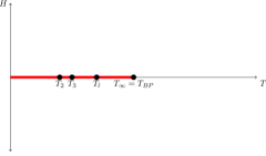
Figure 1: Schematic of the countable infinity of phase transitions of MHZ. The dots correspond to the countable infinity of phase transitions (as one traverses vertically by varying $H$ through $0$ at a given temperature in the ordered phase) of integer order.

Fig 1 carries a schematic of the phase diagram of MHZ. The gist of their approach is to make a careful detailed study of the free energy $F(H,T)$. In a generic ferromagnetic system with a phase transition, $F(H,T)$ is analytic at all points except in the region shown in red: $[H=0,0\leq T\leq T_{BP}]$. In this limit the free energy is given by Müller-Hartmann and Zittartz (1975)

$$F(H,T)=F(0,T)+f_{reg}(H^{2},T)+A(T)|H|^{\kappa},H\to 0,$$ (1)

where the regular part is a function of $H^{2}$ because of symmetry, and the leading singular part $A(T)$ shows a power law behavior. The unusual aspect of the Cayley tree lies in the fact that the critical exponent $\kappa$ varies continuously from $1$ at $T=0$ to $\infty$ Müller-Hartmann and Zittartz (1975) at the usual phase transition called the Bethe-Peierls transition $T_{BP}$. This behaviour is in sharp contrast to most commonly encountered phase transitions where $\kappa$ remains a constant ($=1$ for a first order transition, $2$ for a second order transition and so on). By studying the points at which $\kappa$ takes integer values, they identify a countable infinity of phase transitions which fit into the Ehrenfest classification of phase transitions of integer power-order.

Here we point out that in fact a simple (albeit unusual) set of susceptibilities identify the countable infinity of phase transitions, and indeed a clear physical picture of the meaning behind the phase transitions comes naturally out of them. The susceptibilities turn out to be a product of the zeroth spin with the sum of averages of appropriately grouped spins in the outermost layer of the tree. Furthermore, we can work entirely with the zero-field model, with no requirement of complicated procedures or mathematical methods related to the application of a tiny field followed by taking the zero-field limit.

III The Model

Figure 2: Figure shows a Cayley tree of depth $n=3$ and coordination number $z=3$.

Following the notation of a recent piece of work involving the author Magan and Sharma (2013), we consider the following Hamiltonian:

$$\mathcal{H}=-J\sum_{\langle i,j\rangle}\sigma_{i}\sigma_{j}+H\sum_{j}\sigma_{j},$$ (2)

where the sum involves pairs of spins which are adjacent on the tree (Fig. 2) with coordination number $z$ and depth $n$. $\sigma_{i}$ are Ising variables which can take values $\pm 1$, and J is taken to be positive to make it a ferromagnet. The solution, when the external field is $H=0$, is trivial and we quickly recall it. We introduce new bond variables $\theta_{ij}=\sigma_{i}\sigma_{j}$. The $\theta_{ij}$ can take values $\pm 1$, which make them effectively spin variables too. Specifying all the $\theta_{ij}$, and the spin at the root of the tree $\sigma_{0}$, completely defines the system. The Hamiltonian then takes the following simple form

$$\mathcal{H}=-J\sum_{\langle i,j\rangle}\theta_{ij}.$$ (3)

With the problem now rehashed into one with non-interacting spins under the influence of an external magnetic field, the partition function is readily written down Eggarter (1974):

$$\mathcal{Z}(J)_{Cayley}=2(2\cosh(\beta J))^{N_{b}}=2(2\cosh(\beta J))^{N-1},$$ (4)

where $N_{b}$ is the number of bonds and $N$ is the number of spins, and $\beta=1/T$ is the inverse temperature as usual in equilibrium statistical mechanics. It follows directly Mukamel (1974); Matsuda (1974); Morita and Horiguchi (1975); von Heimburg and Thomas (1974); Magan and Sharma (2013) that the correlation function between any two spins $\sigma_{i},\sigma_{j}$ is given by:

$$\langle\sigma_{i}\sigma_{j}\rangle=\tanh(\beta J)^{d_{ij}}=a^{d_{ij}},$$ (5)

where we define $a\equiv\tanh(\beta J)$ for convenience, and $d_{ij}$ is the distance of the (unique) shortest path between the points $i,j$.

When the external field $H$ is non-zero, there is no simple closed-form expression, however MHZ Müller-Hartmann and Zittartz (1974) write down an infinite-series expansion for the free energy $F(H,T)$, and by a careful, elaborate study of the order in field at which the leading singularity occurs as one crosses zero-field at low-temperature, they obtain the following countable infinity of transition temperatures:

$$T_{l}=\frac{J}{\tanh^{-1}(\frac{1}{\gamma^{(l-1)/l}})},$$ (6)

$l=1,2,\cdots,\infty$, with $l$ being identified as the order of the phase transition within the Ehrenfest scheme. $T_{1}=0$ has a first order phase transition and $T_{\infty}=T_{BP}$ with order infinity is the so-called ‘Bethe-Peierls’ phase transition which is the temperature at which the system first orders as it is cooled down from high temperature. Fig 3 shows a Monte Carlo simulation carried out on a finite-sized system of depth $n=8$ and coordination number $z=3$. We studied the dependence of magnetization as one crosses from negative to positive magnetic field at some of the transition temperatures of MHZ. It seems plausible that in the thermodynamic limit, at a higher transition temperature, a greater derivative of the magnetization with respect to field would diverge at $H=0$. Although the simulations were run on a finite-system the data at $T_{2}$ display a considerably sharp drop near $H=0$ indicative of the diverging derivative, since it is a second order phase transition.

Here we show that the above countable infinity of transition temperatures may be directly obtained from the zero-field model bypassing the elaborate complicated methods of studying the infinite series and the order of divergence of the free energy in the limit of $H\to 0$. We do this by an explicit construction of a special set of ‘susceptibilities’ for the transitions $T_{l}$.

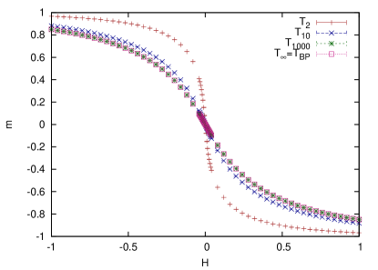
Figure 3: A plot of the magnetization $m=\frac{1}{N}\sum_{i}\langle\sigma_{i}\rangle$ versus magnetic field from Monte Carlo simuations of a finite-sized sytem of coordination number $z=3$ and depth $n=8$. Data are shown for different runs at the MHZ transition temperatures $T_{2},T_{10},T_{1000},T_{\infty}\equiv T_{BP}$. At higher transition temperatures, the curve becomes smoother and smoother indicating that in the thermodynamic limit the singularity would occur at a higher order differentiation with respect to $H$. Since our system is finite, the data are practically indistinguishable for $T_{1000}$ and $T_{\infty}$.

IV Construction of the susceptibilities for the MHZ transition temperatures

In order to construct the susceptibilities for the MHZ transition temperatures, we choose the depth of the lattice to be of the form $n=lp$, where $l$ can take values $1,2,3,\cdots,\infty$. Since we are interested in the $p\to\infty$ limit, no loss of generality is incurred. The number of spins in the $n^{th}$ layer of the tree is $N_{n}=z(z-1)^{n-1}\equiv(1+\frac{1}{\gamma})\gamma^{n}$, where we have defined $\gamma\equiv(z-1)$ for convenience. Let us denote the $n^{th}$ layer spins by $\sigma_{n,1},\sigma_{n,2},\cdots,\sigma_{n,N_{n}}$ in order from left to right, as can be visualized in Fig. 2. Next, we group the first $M_{p}\equiv\gamma^{p}$ spins of the $n^{th}$ layer and call their average $\tilde{\sigma}_{n,1}=\frac{1}{M_{p}}\sum_{i=1}^{M_{p}}\sigma_{n,i}$; we then group the second $M_{p}$ spins of the $n^{th}$ layer and call their average $\tilde{\sigma}_{n,2}=\frac{1}{M_{p}}\sum_{i=M_{p}+1}^{2M_{p}}\sigma_{n,i}$, and so on. By this procedure we form $K_{n,p}\equiv\frac{N_{n}}{M_{p}}$ spin averages:

$$\tilde{\sigma}_{n,j} =\frac{1}{M_{p}}\sum_{i=(j-1)M_{p}+1}^{jM_{p}}\sigma_{n,i}$$ (7)

$$j =1,2,3,\cdots,K_{n,p}.$$

Now we are ready to write down the susceptibilities. Recalling that $\sigma_{0}$ is the spin at the root node, the susceptibilities are simply given by:

$$\mathcal{X}_{l}=\sigma_{0}\sum_{j=1}^{K_{n,p}}\tilde{\sigma}_{n,j},$$ (8)

which is our main result. To see that this leads to the MHZ transition temperatures, let us invoke the two-point correlation functions from the last section to compute the expectation value:

$$\langle\mathcal{X}_{l}\rangle =\langle\sigma_{0}\sum_{j=1}^{K_{n,p}}\tilde{\sigma}_{n,j}\rangle$$ (9)

$$=\sum_{j=1}^{K_{n,p}}\frac{1}{M_{p}}\sum_{i=(j-1)M_{p}+1}^{jM_{p}}\langle\sigma_{0}\sigma_{n,i}\rangle$$

$$=\sum_{j=1}^{K_{n,p}}\frac{1}{M_{p}}\sum_{i=(j-1)M_{p}+1}^{jM_{p}}a^{n}$$

$$={K_{n,p}}a^{n}$$

$$=(1+\frac{1}{\gamma})[\gamma^{(l-1)}a^{l}]^{p}.$$

Therefore we see that as $p\to\infty$,

$$\langle\mathcal{X}_{l}\rangle\to\begin{cases}0&\text{if $\gamma^{(l-1)}a^{l}<1$}\\ \infty&\text{if $\gamma^{(l-1)}a^{l}>1$}.\end{cases}$$ (11)

$\gamma a^{\frac{l}{(l-1)}}=1$ thus defines the $l^{th}$ transition temperature. These are precisely the transition temperatures of MHZ as given in Eqn. 6 Müller-Hartmann and Zittartz (1974); Falk (1975). It is worth pointing out that for $l=2$, this yields the so-called (because of the appearance of the same in the disordered version of the same Hamiltonian Magan and Sharma (2013)) ‘spin-glass’ transition temperature $T_{SG}=\frac{J}{\tanh^{-1}(\frac{1}{\sqrt{\gamma}})}$, and the $l\to\infty$ limit yields the Bethe-Peierls transition temperature $T_{BP}=\frac{J}{\tanh^{-1}(\frac{1}{\gamma})}$.

V Conclusions

We have introduced a set of ‘susceptibilities’ that help identify the mysterious MHZ transition temperatures on the Cayley tree in a transparent manner. They are given by the product of the zeroth spin with an appropriately averaged sum of spins from the outermost layer in a Cayley tree. A clear physical understanding of the phase-transitions emerges naturally. We observe that our susceptibilities have the feature that in the thermodynamic limit, they are zero above the phase transition, but tend to infinity below it. We are able also to identify the second-order phase transition $T_{2}$ as the phase transition known as the spin-glass phase transition in the literature.

Furthermore, although we have concentrated on the Ising ferromagnet here, the susceptibilites defined here are primarily attached to the geometry of the lattice. Therefore, they should be applicable much more generally: for example with $m$-component vector spins and the bonds could be ferromagnetic or antiferromagnetic or disordered. Quantum models should display similar transitions as well: a detailed investigation of various models from this perspective would be desirable.

Finally, we remark that the statistical mechanics problem on the tree has been connected with the problem of reconstruction of information on trees in formal, extensive studies Mézard and Montanari (2006); Mossel (2004). It would be interesting to understand if and how the MHZ countable infinity of phase transitions would fit into this generalized problem, which might be of interest to a broader community.