The Lyapunov matrix equation. Matrix analysis from a computational perspective††thanks: Version of January 10, 2015. This work is a contribution to the Seminar series “Topics in Mathematics”, of the PhD Program of the Mathematics Department, Università di Bologna.
Abstract
Decay properties of the solution to the Lyapunov matrix equation are investigated. Their exploitation in the understanding of equation matrix properties, and in the development of new numerical solution strategies when is not low rank but possibly sparse is also briefly discussed.
keywords:
sparsity pattern, banded matrices, Kronecker products, exponential decay.AMS:
65F50, 15A091 Introduction
We are interested in the analysis of the linear matrix equation
| (1) |
to be solved for ; here and in the following denotes the transpose of the matrix . In particular, we focus on the decay and sparsity properties of the involved matrices that can be exploited for computational purposes, or that can give insight into the analysis of numerical solution methods.
Matrix equations have always had a key role in Control theory, because their solution matrix carries information on the stability of the problem [1],[5]. More recently, linear matrix equations and their generalizations, linear “tensor” equations, have been shown to be an appropriate tool to represent the discretization of parameterized partial differential equations, as they arise for instance in stochastic modeling; see, e.g., [3],[21],[16] and the discussion in [29]. Their analysis and numerical solution is therefore attracting considerable attention in the numerical and engineering communities.
Using the Kronecker product, the matrix equation (1) can be rewritten as the following standard (vector) linear system
| (4) |
where the Kronecker product of two matrices and of size and , respectively, is defined as
the vec operator stacks the columns of a matrix one after the other as
From (4) we can deduce that the system admits a solution for any and this is unique, if and only if the matrix is nonsingular. Using a standard result for the spectrum of Kronecker product matrices, this is equivalent to requiring that , where denotes the set of eigenvalues of (see, e.g., [19, Theorem 4.4.6]).
Though the Kronecker form (4) of the problem is appealing, as a large body of literature on linear systems can be exploited, this approach dramatically increases the complexity of the computation, and also cannot preserve the intrinsic properties of the problem in practice; for instance, if is symmetric, then the matrix is also symmetric. This property is not preserved when solving (4), unless the system is solved at a very high accuracy.
The numerical solution of (1) is particularly challenging when is large. Indeed, although and may be sparse and/or structured, the solution matrix is usually dense. For or higher, storing the full matrix becomes prohibitive, and either sparse or low-rank approximations are sought. Experimental evidence and theoretical results indicate that low rank approximations can indeed be sought after whenever the right-hand side is itself a low rank matrix. Major efforts in the past decades have been devoted to determining approximations of the lowest possible rank, given a fixed final accuracy. Interestingly, strategies that determine the most accurate approximation for a given rank have also been investigated. We refer to [29] for a recent survey on recent computational strategies.
Sparsity and decay (quasi-sparsity) patterns of the solution matrix have been less investigated. We aim to explore recent findings in this direction: while decay pattern results are proved by using the closed forms above and thus they seem to be of merely theoretical interest, they may be insightful in the development of computational procedures and in the analysis of the expected solution properties.
Decay properties have been classically investigated for the entries of the inverse of banded matrices. Let , be a symmetric positive definite banded matrix with bandwidth , that is for , and let be the ratio between its largest and smallest eigenvalues. Then Demko et al. [13] showed that
| (5) |
where , and also depends on the extreme eigenvalues of . This bound shows an exponential off-diagonal decay property as the inverse matrix entry moves away from the main diagonal, and the decay depends on the bandwidth of . This property was generalized to functions of symmetric matrices in [7] and more recently to more general matrices and abstract settings in [8],[6].
With completely different purposes (see [10]), in [11] it was shown that also the Lyapunov operator
enjoys similar properties. More precisely, for symmetric and positive definite, the entries of the matrix show a rapid, although not necessarily exponential, decay pattern as one moves away from the element in position . Here we would like to linger over this property, exploring some of its possible consequences both theoretically and computationally. The main aim of this paper is to discuss some recent results, and highlight directions of research that could improve our understanding of the matrix properties of (1), and perhaps encourage the development of new computational strategies for its numerical solution when is not low rank but possibly sparse.
We will first generalize the decay pattern result to a wider class of matrices of interest in applications. Then we will show how to use this decay pattern to characterize the approximate solution matrix of large Lyapunov equations by projection-type methods. Finally, we will make some comments on the solution pattern for sparse .
All reported experiments and plots were performed using Matlab [25].
2 Closed forms of the matrix solution
The solution of (1) may be written in closed form in a number of different ways; here we report the forms that have been used in the literature:
-
Integral of resolvents. The following representation, due to Krein, exploits spectral theory arguments: (see, e.g., [24])
(6) where is the identity matrix and is a contour containing and sufficiently close to the spectrum of .
-
Integral of exponentials. Assume that the field of values111The field of values of is defined as . of is all contained either in or in , excluding the imaginary axis. This representation, due to Heinz, [18, Satz 5], is tightly connected to the previous one,
(7) where is the matrix exponential of .
-
Finite power sum. Assume with , , and let of degree be the minimal polynomial of with respect to , namely the smallest degree monic polynomial such that . Then ([12])
(8) where is the solution of the Lyapunov equation with coefficient matrices given by the companion matrix of , and right-hand side the matrix , where ; see also [23].
-
Similarity transformations. Strictly related to (c), in addition this form assumes that can be diagonalized, . Let . Then
3 Decay pattern properties of the solution
The sparsity pattern of the matrix influences the pattern of the solution to (1), which can be qualitatively described a-priori. This pattern is typical of certain discretizations of elliptic partial differential equations. For instance, when discretizing the Poisson equation on the unit square by means of finite differences or uniform low degree finite elements, the algebraic linear system is obtained, where is called the stiffness matrix, and is symmetric and tridiagonal, ; see, e.g., [14, section 6.3.3]. Clearly, this problem is equivalent to the Lyapunov equation (1) with and . The particular pattern we are analyzing is derived whenever is, say, a single-point forcing term. Analogously, the analysis of the decay pattern in may give insight into the understanding of the sparsity pattern of the stiffness matrix , since each column of , is nothing but the solution to [11]. Our analysis helps formalize the oscillating - while decaying - pattern observed in the inverse stiffness matrix.
Example 1.
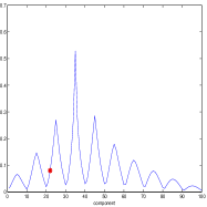
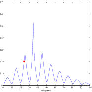
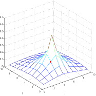
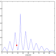
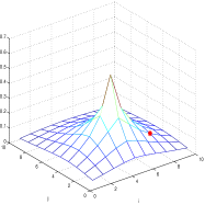
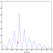
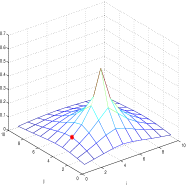
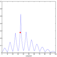
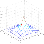
Let , and let , so that , . Figure 1 shows the connection between the column (left plot) and the solution (right plot on the mesh) of the corresponding problem . The plots illustrate the correspondence of each component of the vector as an entry of the matrix , thus describing the oscillating behavior of the column . Note that since is also banded with bandwidth , the overall decay is justified by the estimate in (5), while the Kronecker structure is responsible for the oscillations.

3.1 Decay pattern of the solution matrix
Assume the right-hand side consists of a very sparse matrix, as an extreme case, having a single nonzero element, so that
Without loss of generality, in the following we shall assume that . Then using the integral closed form in (6) we can write
| (9) |
where . Let be the class of -banded matrices of the form with (Hermitian) and , and denote by the line segment containing the eigenvalues of a matrix . Note that if , also the matrix in (9) belongs to . The set includes real symmetric matrices (for and ), but also complex skew-Hermitian matrices ( and ), and complex shifted matrices, as they arise, for instance, in the discretization of the Helmoltz equation. All matrices in are normal matrices, that is for it holds that .
To be able to characterize the decay pattern in the solution , we recall a result derived in [15].
Theorem 2.
Let , and be defined as , with . Then
where, writing ,
with and .
With this result, the following bound for the entries of the Lyapunov solution matrix can be obtained; in spite of the more general setting, the proof proceeds as in [11], and it is therefore omitted.
Theorem 3.
For , let , with eigenvalues contained in the line segment . With the notation of Theorem 2, and for and , , , the following holds.
i) If and , then
ii) If either or , then
iii) If both and , then
Example 4.
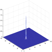
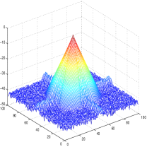
We consider the nonsymmetric tridiagonal matrix , , and with ; note that the same pattern is obtained with its complex counterpart . Figure 2 shows the solution pattern in linear (left) and logarithmic (right) scale. The solution entries decay very quickly away from the entry . This fact can be appreciated by noticing the -axis in the logarithmic scale.
In cases of interest in applications, such as in the case of problems stemming from certain discretizations of elliptic partial differential equations, the matrix itself may have a structure of sum of Kronecker products, that is
| (10) |
where is and banded. We use once again (9) for expressing , by first assuming that a lexicographic order was used to generate the indexes , on the two-dimensional grid, so that we can identify , . Then we can see that the inner product inside the integral satisfies where solves the Lyapunov equation
Therefore, in a recursive manner, the decay of the entries in the matrix can be described in terms of Theorem 3. In practice, this pattern results in a “local” oscillation associated with the decay of the columns of , and a “global” oscillation, associated with the decay of .
Example 5.
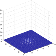
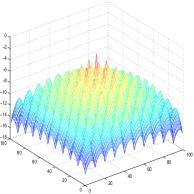
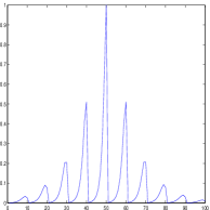
A typical sample of this behavior is shown in Figure 3, where , , so that , and .
Combining the Kronecker structure of with the one in (10) of the Lyapunov equation, we can reformulate the problem as
where , and all identity matrices have dimension . This form reveals the actual tensorial nature of the solution in case has the described Kronecker structure. Computational methods to solve for while using only information in together with the tensor structure have been proposed; see, e.g., [22]. Here we just want to emphasize that the quality of the decay in the entries of , and thus of , is all determined by that of the banded matrix , while the location of this decay pattern is ruled by the Kronecker form of , as nicely visible in the middle plot of Figure 3.
3.2 Numerical low rank properties of the solution matrix
In the literature there is very large experimental evidence that if the right-hand side in (1) has low rank, then the eigenvalues of the solution decay very rapidly. In some cases, such as for symmetric and positive definite, this behavior has been proved [26]. Bounds that cope with non-normality have also been derived, see, e.g., [28, sec.3.1.2] and [2]. Theoretical results showing the fast decay of the spectrum rely on the low rank of the matrix , and on the spectral properties of the coefficient matrix . We are not aware of results that combine the truncation strategies associated with the matrix decay pattern with the low rank property. Both strategies aim at drastically reducing the memory requirements of the solution matrix, and in general, sparsity-driven truncated matrices may have larger numerical rank than the original matrices. However, the following example provides an interesting setting, which will be worth exploring in the future.
Example 6.
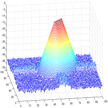
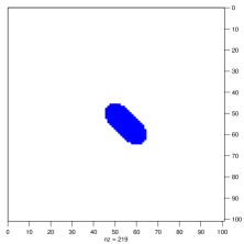
Let , and with . The left plot of Figure 4 shows the solution pattern. The symmetric and positive semidefinite matrix has 9724 nonzero elements. Moreover, 25 eigenvalues of are above , therefore can be very precisely reproduced as with a tall matrix having rank (and thus number of columns) as low as 25. The right plot shows the sparsity pattern of the matrix obtained by zeroing all entries of below (the largest entry of is ). The matrix has precisely 19 nonzero singular values, and only 219 nonzero entries (see right plot of Figure 4). The accuracy of is not as good as with the rank-25 matrix, since , however for most applications this approximation will be rather satisfactory. Though this example is not sufficiently general to make a general case, this phenomenon deserves further analysis.
4 Numerical considerations
Sparsity and quasi-sparsity properties are now starting to be considered in the numerical approximation of the solution to (1). In the following we shall discuss two situations where the analysis of the previous sections can provide insights into the understanding and development of numerical strategies.
4.1 Decay issues in the approximate solution by projection
Let be and sparse, with , . An effective strategy for approximately solving (1) consists of determining a good approximation space of small dimension , and then generating where the orthonormal columns of span . The matrix is determined by imposing some extra condition. For instance, a possible strategy requires that the residual satisfies the following (orthogonality) condition:
Inserting the expression for the residual, and recalling that , this condition leads to the following reduced Lyapunov equation
| (11) |
Setting and , the matrix is thus determined by solving the equation of (small) size ; this can be performed by using a “dense” method, such as the popular Bartels-Stewart algorithm, whose computational cost is [4]. The effectiveness of the whole approximation thus depends on how small can be and still obtain a satisfactory approximation.
The choice of is crucial to obtain a rich enough approximation space while keeping its dimension small. We refer the reader to the recent survey [29] for a comprehensive description of these issues and the relevant recent literature. Here we consider the simplest possible choice of approximation space in the class of Krylov subspace methods: assuming for ease of presentation , we define the (standard) Krylov subspace as the vector space
As increases, is obtained from by one additional multiplication by of the last basis vector. An orthonormal basis can be progressively constructed as increases by using the Arnoldi procedure [27], giving rise to the columns of ; in particular, . The Arnoldi recurrence also establishes the following relation
| (12) |
where is the next vector of the basis, and is computed during the recurrence.
A nice feature of the Arnoldi procedure, is that the reduced matrix is upper Hessenberg, so that the cost of solving the reduced matrix equation in (11) is lower than for a full matrix. For symmetric, the Arnoldi procedure reduces to the Lanczos procedure, and most importantly in our context, is also symmetric and thus tridiagonal. With these hypotheses, the sparsity considerations of the previous sections become relevant. Indeed, the solution to (11) can be written in closed form as
It is also important to keep in mind that a new will be constructed each time the Krylov subspace is enlarged by one, since will be extended to by the addition of one row and one column.
The entries of can be bounded as described in Theorem 3, where however the right-hand side this time has a fixed nonzero entry, the one corresponding to the (1,1) position. Thus,
| (13) |
Since is tridiagonal, and thus banded with bandwidth , the quantities undergo the exponential decay described in Theorem 2, with the rate . Here is associated with the spectral properties of . We recall here that due to the Courant-Fisher min-max theorem, the eigenvalues of tend to approximate the eigenvalues of when is symmetric, therefore the spectral properties of will eventually be associated with those of , as grows.
Remark 7.
Our presentation is based on (13), which exploits decay properties of the inverses of shifted matrices described in Theorem 2. Qualitatively similar results could be obtained by using the exponential closed form in (7), by using very recently developed bounds for the entries of the exponential matrix [9].
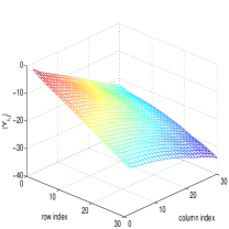
It is important to realize that the presence of a fixed column index in (13) provides additional structure to the decay pattern. For instance, all diagonal entries of have a decreasing pattern, as
so that, using Theorem 3,
where is as described in Theorem 2, with real symmetric. More explicit estimates can be obtained by bounding the integral from above, as done, e.g., in [11]; we avoid these technicalities in this presentation.
The bound above allows us to distinguish between the decay of the entries of and that of the entries of , since in the latter case, the diagonal entries do not necessarily decay. Moreover, the integrand for the nondiagonal entry , will contain the term
illustrating a superexponential decay of the antidiagonals, as grows.
Example 8.
In Figure 5 a typical pattern is shown for : for this example, , is the finite difference discretization of the two-dimensional Laplace operator in the unit square with homogeneous boundary conditions, and is taken to be a vector with random uniformly distributed values in the interval . A standard Krylov subspace of dimension was considered, so that is a real symmetric matrix.
The analysis of the decay pattern of appears to be new. On the other hand, it is well known that the last row (or column) of carries information on the accuracy of the solution . Indeed, let be the Frobenius () or induced 2-norm () of the matrix . Then using (12) the residual norm satisfies (see [29])
where in the last equality the orthogonality of the columns of , and (11) were used. Hence,
Therefore, if the last column of , , is small in norm then the residual will be small. We note that on the other hand, the possibility that is small is related to the fact that an invariant subspace is found while generating the space via the Arnoldi recurrence (12), which is in general a less likely event, for general and small compared to .
Due to the previous discussion on the entries , for the vector is expected to be small for large enough (we recall here that changes and increases its dimension as increases). For the norm is bounded as
Using , after some algebra we obtain
where we used that . More explicit estimates could be obtained by further bouding the integrand in terms of the variable .
The relation between the convergence rate, in terms of the residual norm, and the solution sparsity pattern should not come as a surprise. Indeed, the estimate in Theorem 2 exploits the same polynomial approximation properties that are used to prove convergence of standard Krylov subspace methods to solve the Lyapunov equation by projection [30].
4.2 Numerical solution for a sparse right-hand side
Projection type methods are suitable when the right-hand side matrix has low rank, as discussed in the previous sections. Sparse but larger rank right-hand sides can also enjoy particular properties, and may also be viewed as sum of low rank matrices. For instance, assume that is symmetric positive definite and banded. Due to the linearity of the matrix equation, the solution to
| (14) |
can be split as , where for all such that the addend matrix is the solution to the corresponding equation
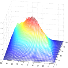
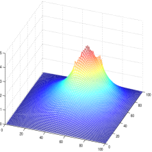
see, e.g., [20] for a similar linearity strategy. It follows from our discussion on decay that each will have an a-priori detectable decay pattern - a peak corresponding to the entry - from which the decay pattern of the whole of can be predicted; see, e.g., [17] for a similar discussion on the sparsity property of the resulting solution. We remark that our decay analysis suggests that each may be truncated to maintain sparsity in the approximate solution , so as to obtain a good enough sparse approximate solution . We next report a typical example; see also Example 6.
Example 9.
For equal to the Laplace operator as before, the left plot of Figure 6 reports the solution to (14) when is a nonsingular diagonal matrix with random entries uniformly distributed in the interval (0,1); the right plot corresponds to with equal to a random value as above, but only for . The different sparsity patterns of the two solutions is as expected from the theory. In particular, the left plot shows slightly larger values of the diagonal entries corresponding to the central part of the diagonal, where all linear components contribute. On the other hand, the right plot confirms that (diagonal) peaks can only occur in correspondence with the nonzero diagonal entries of .
5 Further considerations
Our presentation was aimed at highlighting some decay properties of the matrices involved in the solution of the Lyapunov equation, that may give insight into the development of new numerical methods. In particular, the solution of the matrix equation when the right-hand side matrix has large or even full rank remains a big challenge. Exploiting the possible sparsity of may provide a good solution strategy; we refer the reader to [17] and its references for recent developments in this direction.
For ease of presentation, our analysis was limited to the Lyapunov equation. Very similar results can be obtained for the Sylvester linear equation , where may be of different dimensions; indeed, the solution can be written with a closed form similar to that in (6), so that corresponding decay bounds can be obtained; see [29].
References
- [1] A. C. Antoulas. Approximation of large-scale Dynamical Systems. Advances in Design and Control. SIAM, Philadelphia, 2005.
- [2] A. C. Antoulas, D. C. Sorensen, and Y. Zhou. On the decay rate of Hankel singular values and related issues. Systems & Control Letters, 46(5):323–342, August 2002.
- [3] I. Babuska, R. Tempone, and G. E. Zouraris. Galerkin finite element approximations of stochastic elliptic partial differential equations. SIAM J. Numer. Anal., 42(2):800–825, 2004.
- [4] R. H. Bartels and G. W. Stewart. Algorithm 432: Solution of the Matrix Equation . Comm. of the ACM, 15(9):820–826, 1972.
- [5] P. Benner, V. Mehrmann, and D. Sorensen (eds). Dimension Reduction of Large-Scale Systems. Lecture Notes in Computational Science and Engineering. Springer-Verlag, Berlin/Heidelberg, 2005.
- [6] M. Benzi and P. Boito. Decay properties for functions of matrices over C* -algebras. Lin. Alg. Appl., 456:174–198, 2013.
- [7] M. Benzi and G. H. Golub. Bounds for the entries of matrix functions with applications to preconditioning. BIT Numerical Mathematics, 39(3):417–438, 1999.
- [8] M. Benzi and N. Razouk. Decay bounds and algorithms for approximating functions of sparse matrices. ETNA, 28:16–39, 2007.
- [9] M. Benzi and V. Simoncini. Decay properties of functions of matrices with Kronecker structure. In preparation, Dipartimento di Matematica, Università di Bologna, 2015.
- [10] C. Canuto, V Simoncini, and M. Verani. Contraction and optimality properties of an adaptive Legendre-Galerkin method: the multi-dimensional case. J. Scientific Computing, v.xx:p.xx, 2014. To appear.
- [11] C. Canuto, V. Simoncini, and M. Verani. On the decay of the inverse of matrices that are sum of Kronecker products. Lin. Alg. Appl., 452(1):21–39, 2014.
- [12] E. de Souza and S. P. Bhattacharyya. Controllability, Observability and the Solution of . Lin. Alg. Appl., 39:167–188, 1981.
- [13] S. Demko, W. F. Moss, and P. W. Smith. Decay rates for inverses of band matrices. Math. Comp., 43:491–499, 1984.
- [14] J. W. Demmel. Applied Numerical Linear Algebra. SIAM, 1997.
- [15] R. Freund. On polynomial approximations to with complex and some applications to certain non-hermitian matrices. Approx. Theory and Appl., 5:15–31, 1989.
- [16] D. Furnival, H. Elman, and C. Powell. H(div) preconditioning for a mixed finite element formulation of the stochastic diffusion problem. Mathematics of Computation, 79:733–760, 2010.
- [17] A. Haber and M. Verhaegen. Sparse solution of the Lyapunov equation for large-scale interconnected systems. Technical report, Delft University of Technology, 2014. arXiv:1408.3898.
- [18] E. Heinz. Beitrage zur Storungstheorie der Spektralzerlegung. Math. Annalen, 128:373–411, 1955.
- [19] R. A. Horn and C. R. Johnson. Topics in Matrix Analysis. Cambridge University Press, Cambridge, 1991.
- [20] D. Y. Hu and L. Reichel. Krylov Subspace Methods for the Sylvester Equation. Linear Algebra and Appl., 172:283–313, July 1992.
- [21] B. N. Khoromskij. Tensors-structured numerical methods in scientific computing: survey on recent advances. Chemometrics and Intelligent Laboratory systems, 110:1–19, 2012.
- [22] D. Kressner and C. Tobler. Krylov subspace methods for linear systems with tensor product structure. SIAM J. Matrix Anal. Appl., 31(4):1688–1714, 2010.
- [23] P. Lancaster, L. Lerer, and M. Tismenetsky. Factored forms for solutions of and in companion matrices. Lin. Alg. Appl., 62:19–49, 1984.
- [24] P. Lancaster. Explicit solutions of linear matrix equations. SIAM Review, 12(4):544–566, 1970.
- [25] The MathWorks, Inc. MATLAB 7, r2013b edition, 2013.
- [26] T. Penzl. Eigenvalue decay bounds for solutions of Lyapunov equations: the symmetric case. Systems and Control Letters, 40(2):139–144, 2000.
- [27] Y. Saad. Iterative methods for sparse linear systems. SIAM, Society for Industrial and Applied Mathematics, 2nd edition, 2003.
- [28] J. Sabino. Solution of Large-Scale Lyapunov Equations via the Block Modified Smith Method. PhD thesis, Rice University, 2006.
- [29] V. Simoncini. Computational methods for linear matrix equations. Technical report, Alma Mater Studiorum - Università di Bologna, 2013.
- [30] V. Simoncini and V. Druskin. Convergence analysis of projection methods for the numerical solution of large Lyapunov equations. SIAM J. Numer. Anal., 47(2):828–843, 2009.