Random Field Ising Model in two dimensions: Bethe approximation, Cluster Variational Method and message passing algorithms
Abstract
We study two free energy approximations (Bethe and plaquette-CVM) for the Random Field Ising Model in two dimensions. We compare results obtained by these two methods in single instances of the model on the square grid, showing the difficulties arising in defining a robust critical line. We also attempt average case calculations using a replica-symmetric ansatz, and compare the results with single instances. Both, Bethe and plaquette-CVM approximations present a similar panorama in the phase space, predicting long range order at low temperatures and fields. We show that plaquette-CVM is more precise, in the sense that predicts a lower critical line (the truth being no line at all). Furthermore, we give some insight on the non-trivial structure of the fixed points of different message passing algorithms.
I Introduction
Many of the thermodynamic properties of the Random Field Ising Model (RFIM) remained controversial for more than 40 years. In particular the existence or the absence of a spin glass phase in the model attracted a lot of attentionC. De Dominicis et al. (1995); Mézard and Monasson (1994); Brézin and De Dominicis (2001); de Almeida and Bruinsma (1987); Pastor et al. (2002); Fytas and Martín-Mayor (2013); Picco and Sourlas (2014). Only recently we found confirmation that this spin glass phase is possible only if the magnetization of the system is constrained to be fixed Krzakala et al. (2010). Without this constraint, the RFIM possesses only a paramagnetic-ferromagnetic transition when or no transition at all in Krzakala et al. (2010, 2011); Imry and Ma (1975); Aharony et al. (1976).
These results bring new questions into the field. For example: Why standard perturbation theory fails? Could the spin-glass phase, deduced for the model with fixed magnetization in the Bethe lattice Krzakala et al. (2010), have some role in the dynamical behavior of models in finite dimensions? Do message passing algorithms always converge in lattices of finite dimensions as occurs in the ferromagnetic Ising model Domínguez et al. (2012)?
On the other hand, our current knowledge about the model makes it a good starting point to improve the comprehension about the applicability and the capabilities of techniques that have being used to study this and other disordered systems. Of special interest is the analytical solution by Mézard and Parisi Mézard and Parisi (2001, 2003) of the Viana-Bray model Viana and Bray (1985)) within a Replica Symmetry Breaking ansatz. Since then, the field has progressed very fast. First, the ansatz was rapidly extended to other models Mezard et al. (2002); Mézard and Zecchina (2002); Mulet et al. (2002). Then, it was soon recognized the connection between this approach and message passing algorithms, the well-known Belief Propagation (BP) algorithm Pearl (1988) corresponds to the Bethe approximation of the free energy of a specific modelKabashima and Saad (1998).
To go from the Bethe approximation to methods that considered loops in the interaction networks turned out to be a more difficult task Montanari and Rizzo (2005); Chertkov and Chernyak (2006a, b); Mooij and Kappen (2007); Gomez et al. (2010); Jing-Qing Xiao (2011); Haijun Zhou and Bi (2011); Haijun Zhou (2013). An important step in that direction came from Yedidia and co-workers Yedidia et al. (2005a) that described how to generalize the Cluster Variational Method (CVM) of Kikuchi Kikuchi (1951). The minimization of the CVM free energy can be achieved by the use of a Generalized Belief Propagation (GBP) algorithm Yedidia et al. (2005a), although the solution found is always Replica Symmetric(RS).
More recently it was possible to merge the CVM with the Replica Symmetry Breaking (RSB) ansatzRizzo et al. (2010). Although, technically involved, the approach allowed the study of the Edward-Anderson (EA) model in two dimensions. In this system it was possible to unveil the connection between the phase transition predicted by the average case scenario and the properties of the Generalized Belief Propagation algorithm in two dimensional latticesLage-Castellanos et al. (2013). Running standard BP for the Bethe approximation in EA 2D one finds a paramagnetic solution at high temperature, as expected. However, decreasing temperature BP finds, not one, but many fixed points with non-zero local magnetizations. Suggesting then, a transition from a paramagnetic to an spin glass phase that although is not expected in thermodynamical grounds, is nevertheless predicted within the approximation and connected with the performance of message passing algorithms Dominguez et al. (2011); Lage-Castellanos et al. (2013). Furthermore, these low temperature fixed points are also correlated with the metastable states of the Monte Carlo dynamics of the model Lage-Castellanos et al. (2014).
In this work we present the equations describing the RFIM within the CVM at the RS level. The goals are, on one side, to compare the predictions that can be derived from the equations with our current knowledge about the model. This should shed light on the limitations and advantages of the approximation itself. On the other, to extend the connection already established within the EA model between these average case equations and message passing algorithms. In particular, we will focus on whether the CVM at the Bethe and plaquette level also predict a spin-glass phase, and if this is connected with the behavior of message passing algorithms.
The rest of the work is organized as follows. In the next section II, we present the model. In section III we obtain message passing equations for the single instances of the model, both at the Bethe (BP) and the plaquette level of CVM (GBP). The phase diagram obtained by implementing these belief propagation algorithms is discussed in IV. In section V we derive average case predictions at replica symmetric level for both approximations. We summarize and discuss our findings and conclusions in VI.
II The Model
The Random Field Ising Model is a natural extension of the standard Ising ferromagnet to consider the disorder of real solids. Due to a number of reasons, spins in a crystalline lattice are under the influence of small local magnetic fields; intensity and direction of these fields varies rapidly from one site to another uncorrelatedly. This situation can be modeled in a simplified way by considering the following Hamiltonian:
where the first sum runs over all couples of neighboring spins (first neighbors on the lattice) and the second over all sites (spins). We will deal in this work with spins in a bidimensional square lattice, but extensions to more dimensions is conceptually straightforward, although probably numerically cumbersome. The magnetic exchange constants between spins is fixed to (more precisely ) and the spins are the dynamic variables. The disordered local field are a set of random variables generally drawn from a zero-mean bimodal or Gaussian distribution. In our case, a bimodal distribution will be used:
Local fields introduce what is called quenched disorder Parisi et al. (1987): fields and spins are considered to vary in completely different time scales in real solids. Thus, an instance of this model corresponds to a particular realization of the fields. We will use the field intensity as one of the model parameters.
The statistical mechanics of the RFIM model, at a temperature , is given by the Gibbs-Boltzmann distribution
is a normalization constant, called partition function since it depends on the temperature and all other relevant parameters of the model, like for instance.
Finding the exact free energy of a particular sample of our model is quite difficult, because the partition function involves an exponential number of computations, being only accessible to very small systems. However, the interesting limit is the thermodynamic one (), and from a physics perspective we are mostly interested in a description of the ensemble of instances, not in a particular one. Using the replica method for models in fully connected or very sparse random topologies (see Parisi et al. (1987) for a primer), the structure of equilibrium states for the average case can be described in a well defined hierarchy of approximations. The whole approach is based on the idea that the free energy is a self-averaging quantity, so averaging over disorder must match results for real samples when . An exact solution to disordered models in finite dimensions, however, remains immune to analytic results, and usually is treated by simulations or approximations, like the ones described next.
III GBP equations for plaquette-CVM
The fundamental idea behind Generalized Belief Propagation Yedidia et al. (2005a), or Cluster Variational Method Yedidia et al. (2005b); Pelizzola (2005), or Kikuchi approximation Kikuchi (1951) to the free energy of a model is to replace the exact functional free energy by an approximation consisting on the sum of local (small regions) free energies:
Since the set of regions is in principle arbitrary, some regions might contain smaller regions, and therefore an appropriately chosen counting number is used to avoid overcounting free energy contributions Yedidia et al. (2005b). Only in very particular cases a partition like this remains exact (like in the Bethe approximation on tree like topologies) or even an upper bound of the real free energy Yedidia et al. (2005b).
Ideally the distributions minimizing should coincide with the marginals of the exact Boltzmann distributions , but generally (and hopefully) they will only be an approximate of them, and therefore are usually called beliefs and represented by , leaving for the exact marginals.

Though very general, there are specific ways to define the set of regions for approximating the free energy. According to the CVM prescription Kikuchi (1951); Yedidia et al. (2005b), for instance, this set is formed from a primary set of larger regions . Then adding to them the set , formed by the intersections of every pair of regions in . Then adding the intersections of regions in and so on and so forth until no intersections are left, obtaining .
Bethe approximation is just a particular case of CVM where the larger regions considered are the interacting pairs of spins (links). In this work we use Bethe approximation, and, to go beyond, we also use the approximation starting from plaquette regions. A plaquette region is formed by the four spins and links lying on a basic square cell of the lattice (see Fig. 1), and has the advantage over Bethe approximation of including the shortest loops in the graph. It is known that loops are the cause of failure of Bethe approximation. Two adjacent plaquettes overlap in a link region, formed by two neighbor spins and the interaction between them. Two link regions with a common spin overlap in a spin region. Therefore, our approximation contains contributions of free energies from all plaquettes (), links () and sites () (Fig. 1). The free energy approximated with this set of regions is usually called Kikuchi approximation Kikuchi (1951); Pelizzola (2005):
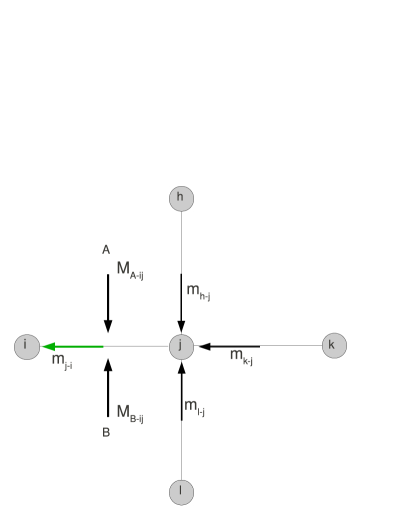
Minimization of this free energy with respect to the beliefs has to be done while keeping the consistency among them, in the sense that distributions on larger regions have to marginalize onto the smaller regions that are part of them. This constrained minimization is implemented via Lagrange multipliers and enforcing plaquette to link and link to spin consistency respectively. The self consistent equations for the Lagrange multipliers are interpreted as message passing equations. The message from link to spin, say, is updated according to:
| (1) |
where is the set of regions of whom is a child. In Fig. 2a it is shown the configuration of all messages involved in updating . The interactions appear as , where . The product over link-to-spin messages runs on , which is the set of links having the site as a child, excluding . In the case shown, includes , and .
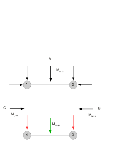
For messages from the square plaquette to link (see Fig. 2b) we have the update equation (2) that is similar in structure. This time, however, on the left hand side appears the product of two link messages that are internal to the plaquette. Normally it is advisable (for convergence issues) to update these first before updating .
| (2) | |||||
Here, is the set of links in plaquette , represents the links that are parent to spin and is the collection of parent plaquettes to .
Messages are the usual representation of the Lagrange multipliers in the context of belief propagation algorithms. However, physically it is nicer to think in terms of cavity fields Mézard and Parisi (2001, 2003), acting from one part of the system onto another. In terms of these fields, messages are recovered as
| (3) |
Only one parameter is enough to represent messages, while for we need three: , and Rizzo et al. (2010); Lage-Castellanos et al. (2011); Dominguez et al. (2011). The update equations for the cavity fields are obtained with little effort. Below we write them using the labeling of Fig. 2.
| where | ||||
Fields define a new effective and coupling constant . For plaquette-to-link fields we get
| (5) | |||||
where
The set of self consistent equations defining messages can be solved by a fixed point iteration. This procedure is known as a message passing algorithm. Standard Belief Propagation (BP) is just a special case for the Bethe approximation. Many details about the implementation of BP and GBP can be found in Dominguez et al. (2011). If the algorithm happens to find a fixed point (convergence is not guaranteed), you can recover the local approximated marginals in terms of the messages, just like with any standard Lagrange multiplier minimization.
Now that we have presented in broad terms the essential features of BP and GBP, we can move to discussing the results when running these fixed point methods on singular instances of 2D RFIM.
IV Results for single instances
Region graph approximation to the free energy and the corresponding message passing algorithms give numerical (estimate) values to all thermodynamic quantities like free energy, energy or entropy. Usually these approximations are compared with Monte Carlo simulation results, or exact predictions (when available). We are most interested in the phase diagram of the model.
Two relevant parameters characterize the random field Ising model: the temperature and the external field intensity . Local fields are scaled by , and with equal probability. The model with is no other than the usual Ising ferromagnet.
Phase Diagram
We know in advance the dominant thermodynamical phase of some particular points in the plane. For instance, at any finite field intensity , and high enough temperature , the free energy minimization is dominated by the entropic term, and therefore spins are mostly uncorrelated (true when ) with vanishing local magnetizations, , and with global zero magnetization given the random origin of the fields .
At zero temperature, the free energy is dominated by the minimization of the energetic term, and at least for , the interaction with the 4 surrounding spins at any given site cannot overcome the interaction with the local external field. In such case, the ground state of the system is trivially . The system is frozen and again global magnetization is zero (except for fluctuations). Let’s call this phase paramagnetic in spite of spins been magnetized. In this sense, paramagnetic refers to the fact that no long range order exists, and the frozenness of the spin is not a collective phenomena but a result of their interaction with external local fields.
Therefore, in both extremes, high and high , the system is paramagnetic, and this is correctly reproduced by both, Bethe and CVM approximations, on single instances (see below). To signal the onset of long range correlations we have used the global magnetization as the order parameter and a threshold value . The value of this threshold can be fixed according to the following reasoning. For a given temperature, long range order, if present, is destroyed for large . In this regime, magnetization is of order . If the system remains paramagnetic when decreasing , magnetization should decrease too. On the contrary, if for lower states with are found, it can be interpreted as the emergence of order in the system. In practice, a value of fits known results for , namely the para-ferro transition point of the Ising model.
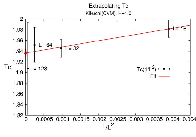
To unveil the phase diagram in the thermodynamic limit from simulations on finite size instances we considered that, for a given value of the field, the mean value of the critical temperature over many samples depends on the system size, . In order to obtain an estimate of the value in the limit, we propose and extrapolate (see figure 3).
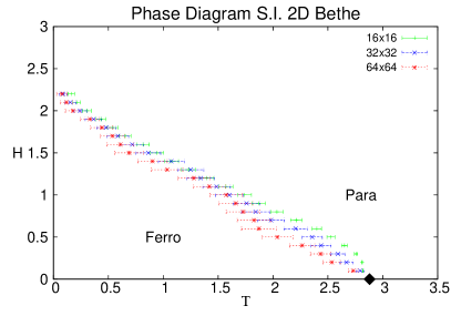
Summarizing, in figures 4 and 5 we show the average phase diagram over many samples of RFIM with different system sizes and the critical line after extrapolation. Our Bethe and CVM calculations predict the appearance of long range correlation in the magnetization of spins at low temperatures and low external fields. This phase (thermodynamically incorrect for ) will be called ferromagnetic. In both cases the para-ferro border starts at the corresponding critical point of the ferromagnetic (non disordered, ) model. This transition is at odds with the rigorous result proving that in even the smallest (random) external field should destroy all chances of a long range order Imry and Ma (1975); Aharony et al. (1976); Bricmont and Kupiainen (1987).
It is not a surprise that mean field approximations stabilize non relevant phases, as it does in the Edwards-Anderson model Dominguez et al. (2011); Lage-Castellanos et al. (2013). This is a general price we pay for implicit factorization at certain levels of the correlations when writing the free energy approximated by regions.

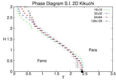
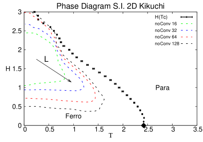
In the CVM plaquette approximation, we faced severe convergence problems that we solved partially by fixing the gauge invariance of message passing equationsDominguez et al. (2011) as explained in appendix VII. In the following, CVM approximation refers to this gauge fixed implementation of the message passing. However, even in this case, there is an island of non convergence for low temperatures and intermediate values of field (see 5).
This region of non convergence grows with the system size. In Fig. 5b we show, for different values of the border of the area where the probability of convergence drops abruptly. As increases, the non convergence island apparently spreads all over the ordered phase. To be more quantitative on this point we plotted for a fixed in Fig. 6a the value of at the frontier for each . The functional dependence of this curve is very well fitted with the law . This suggests that indeed, for large enough lattices the non convergence region moves down to .
Also, for a fixed , we fitted in Fig. 6b the temperature at the convergence border. The form of in this case agrees with . The limit is close to the average critical temperature found by GBP for the same field intensity, . These results enable us to speculate that in the thermodynamic limit the difficulties in convergence would cover all the unphysical ordered phase. Moreover, this also suggests that at least for this model the convergence of GBP is linked to the para-ferro phase transition and may be useful in defining its location.


Multiple solutions: a one case study
For many years there was a strong debate about whether a spin glass phase was present in an intermediate area of the phase diagram just around the border of the para-ferro transition Imry and Ma (1975); Aharony et al. (1976); Bricmont and Kupiainen (1987). Although we now know that long correlation order is impossible in this case, such belief was supported by perturbative and non perturbative replica field theory resultsC. De Dominicis et al. (1995); Brézin and De Dominicis (2001); Parisi and Dotsenko (1992). On the other hand, although numerical Monte Carlo simulations suffer from a strong slowing down near the transition, no evidence of a SG phase is found in either the bimodal or the Gaussian version of the RFIMNewman and Barkema (1996); Middleton and Fisher (2002); Parisi, G. et al. (1999).
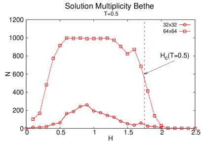

It is consistent with such expectation the fact that Bethe approximation finds many different solutions in the vicinity of the para-ferro transition. They are discerned easily by their different magnetizations. In Fig. 7 we show the number of different solutions found in a system of and at and . The message passing is started from random initial conditions times for each value of the external field intensity. Changing the external field means varying only its intensity while keeping directions on each site. As expected. the larger the system the more solutions are found by the algorithm. Also, for lower temperatures the number of solutions increase, as new local energy minima get stabilized. Notice that multiplicity of solutions appears for and below, within the long range order phase. As a consequence, a proper definition of the critical field/temperature with a threshold in the global magnetization is even more difficult than discussed previously.
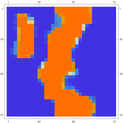


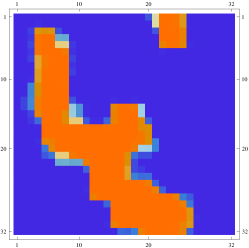
Different Bethe solutions are not completely uncorrelated. They differ in blocks of spins that switch directions from one solution to the other, as shown in Fig. 8. It has been shown for other models, like the Edwards-Anderson in 2D, that these solutions might be connected with the regions of the phase space in which the Monte Carlo dynamics spend more time, or say in other words where the Boltzmann measure concentratesLage-Castellanos et al. (2014). It is to be checked in future works whether this property holds for the RFIM too.
Furthermore, we wonder if this multiplicity of states is truly a sign of a spin glass like behavior for finite lattice sizes, or also an artifact of the Bethe approximation. More precisely, we want to check if it is also a feature of plaquette-CVM approximation. Surprisingly it is not. In most systems studied, only one GBP fixed point was found. In some of them, two or at most three solutions were found. When more than one solution is found, they are still related by the flipping of entire blocks of magnetizations. The drastic reduction of fixed points for plaquette-CVM is conspicuous, and might be interpreted as a sign of the non thermodynamic relevancy of the many Bethe solutions. This is in accordance with the general belief that CVM yields more accurate results than Bethe approximation.
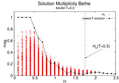
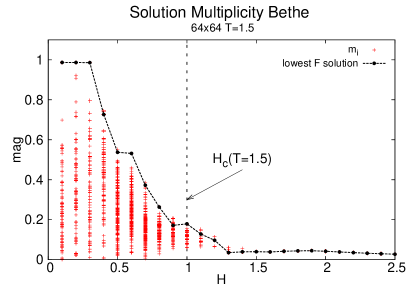
This detailed study of the Bethe and CVM approximations shows the difficulties affronted in defining a critical line in the random field Ising model. At variance with the Ising ferromagnet, where the Bethe and CVM approximations give a clear zero magnetization in the paramagnetic phaseDomínguez et al. (2012), here there are non zero magnetizations at every temperature and field, and the onset of long correlation is further obscured by the appearance of many solutions. It would be more justified if one could define the critical line studying a threshold magnetization value for the solution with lowest free energy at every . The different magnetization values for a 64x64 sample are plotted in Fig. 9. Solutions with the lowest free energy are joined with a solid line. Applying the threshold criteria to this line should improve the quality of the results. However, this requires running message passing thousands of times from random initial conditions for each system, and then the average over thousand of systems. This is a highly resource-consuming task. Instead, we turned to the prediction of a critical line by average case calculations of both Bethe and plaquette-CVM approximations.
V Average case predictions
There are two different procedures to analyze the average case solution of CVM approximations, one more formal relying on the replica method Rizzo et al. (2010) and quite involved, and another more intuitive based on population dynamics Lage-Castellanos et al. (2013). In the case of the Bethe approximation both procedures are equivalent, the latter being a numerical solution of the integral equation appearing in the former Mézard and Parisi (2001). A detailed explanation of both procedures can be found in Lage-Castellanos et al. (2013), and we will only describe them shortly.
Replica-CVM is a formal way of averaging the disorder in the partition function of a region graph approximated disordered model, based on the replica trick Rizzo et al. (2010). As usual in replica method, the average over the disorder couples the replicas, and some ansatz is needed to take the limit. Generalizing the approach in Monasson (1998); Kabashima (2005) to the plaquette-CVM case, this ansatz is a parametrization of messages and in terms of two types of field distributions and respectively:
| (6) | |||||
| (7) |
Minimizing the replicated free energy in terms of these distributions, we obtain two self consistent equations for and :
with and functions defined in (III) and (5) and
All the thermodynamics is encoded into the functions and . The solution of this system is technically involved. Standard population dynamics is not easily applicable because of the need of numerical deconvolution methods (like Fourier transform) to extract from the convolution in the left side of Eq(V). In the case of zero external field and high , however, there is the trivial solution , and , with satisfying a simplified version of the integral equation (V) (see Lage-Castellanos et al. (2013) for details).
We reproduce the stability analysis of the paramagnetic solution for the RFIM, knowing in advance, that is not a good guess in the zone, since at any finite temperature the local magnetizations are non zero, and therefore, messages should be non trivial even in the paramagnetic phase. Around the paramagnetic solution the self consistent integral equations (V) can be linearized for the first moments of the distributions and , and the critical temperature is defined as the moment when the system becomes singular Lage-Castellanos et al. (2013).
In the simplest case of the Bethe approximation, only an equation like the first one in (V) appears (excluding the presence of the functions), and it can be solved again in terms of the moments around , or numerically as a fixed point dynamic over a population of fields representing Mézard and Parisi (2001).

This population sampling method can be extended to the CVM approximation in a less trivial way. A representation of with a population of fields is not enough to attempt a numerical solution of equation (V), since it is not trivial how to deconvolve in the left hand side of (V). Still, you can pretend that a random sampling of and populations and the evaluation of message passing equations (III) and (5) with random local external fields represents a randomized version of the actual message passing occurring in the system, and therefore represents an average system.
In the single instance case, for every update step of messages, it is necessary to update simultaneously the two () messages that enters in the left hand side of (2)Yedidia et al. (2005a). It is prudent then to respect this correlation in the random sampling procedure. In order to do so, a random object containing a and two is defined (see Fig. 10, left). It is possible to generate a new set of and by sampling four of these objects from a large population and using them as the messages acting on a plaquette (see Fig. 10, right). This newly generated random object is added back to the population at the end of each iteration step.
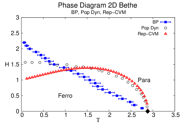
In the population dynamic method we will define the critical temperature as the moment in which the population of fields develop a global magnetization. This means that the balance between positive and negative fields is skewed to one side, signaling the appearance of long range order.
In Fig. 11 we show the critical lines obtained by examine single instances of RFIM in 2D with the Bethe approximation (same data as in Fig. 4b), and the results obtained in average case by both procedures: stability analysis of linearized equation and population dynamics. Remember that for the Bethe case these two methods attempt to solve the same integral equation. Therefore, had the stability analysis been performed to all orders, it would have matched population dynamics results. Nevertheless, for small , a good agreement is observed in Fig. 11. In the limiting case all results agree on the same critical temperature, which can be found accuratelyDomínguez et al. (2012). In presence of disorder, on the other hand, the single instance critical line predicts for the same field intensity a transition temperature which is lower than the average case values. This divergence is closely related to the domain formation picture, because the system needs lower temperatures to be completely magnetized.
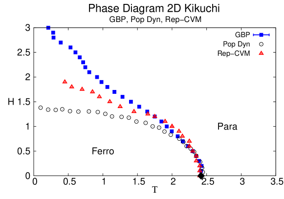
The same comparison is done in Fig. 12 for the plaquette-CVM approximation. Again, at low both average case calculations coincide. Furthermore, they coincide also with the results for the phase diagram obtained within the single instance scenario.
At this point it is interesting to compare these results for CVM with previous predictions for the EA model Lage-Castellanos et al. (2013). Unfortunately the replica stability analysis in RFIM can only be accurate in the low field zone, restricting our analysis to this part of the diagram. While in the 2D EA model the population dynamic and the replica stability give different transitions temperatures, the first one related to the appearance of non paramagnetic GBP solutions and the second pointing the lack of convergence of the message passing, in RFIM both methods seems to coincide (in the low H region). They also coincide with the appearance of magnetized solutions in single instances, and asymptotically with the lack of convergence for . In this sense the relation of single instance behavior of GBP and both average case methods is connected in a similar fashion as in 2D EA. The rest of the diagram (higher ) is harder to analyze, since replica stability is a priori wrong, and population dynamics gets into the non convergent region of single instances.
VI Conclusions
The Random field Ising model is a paradigmatic disordered model in statistical mechanics whose full comprehension in general dimensions resists analytic methods and poses major simulation difficulties. We have studied two approximations to the free energy of this model in 2D, namely Bethe and plaquette-CVM approximations, both in single instances and in the average case.
The qualitative panorama of both approximations is consistent. BP and GBP on finite size instances and average case calculations predict transitions to an ordered phase in a region of low temperatures and low fields. Although it is known that this phase is thermodynamically unstable, the prediction of long range order in 2D is not a surprise, since mean field like approximations tend to stabilize ordered phases. However, Bethe and CVM differ in many aspects. The Bethe approximation predicts a critical line that is above the one of the plaquette-CVM, which is consistent with the expectation that a more precise approximation yields results closer to reality (no critical line at all). On single instances the Bethe approximation converges to many solutions and GBP to only one or at most a few ones related by flipping large spin clusters. Moreover, our results suggest that GBP does not converge for large enough lattices and more important, at least for small values of the field , the non-convergence seems to coincide with the para-ferro transition temperature predicted by the population dynamic and the replica stability analysis. As in the 2D EA model, the behavior of GBP is closely connected with the average case prediction.
VII Appendix: Gauge invariance of GBP equations
GBP equations enforce the correct marginalization of the expectations (beliefs) at each level onto the expectation at its children levels, in a region graph approximation to the free energy of a model. As discussed in Yedidia et al. (2005b), each marginalization requires a Lagrange multiplier, and the self consistency of this multipliers becomes the usual message passing algorithm.
When implementing GBP in single instances, it makes no damage if some of the constraints are forced more than once. For instance, if a plaquette’s belief is forced to marginalize onto two of its links and , then the marginals of these two beliefs must be consistent on variable . Therefore, if one of them, lets say is forced to marginalize on the belief , then it is unnecessary to force the other to marginalize on it, since it inevitably does.
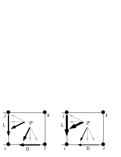
This means that the general prescription for implementing GBP in Yedidia et al. (2005b) is redundant, and the introduced messages or their equivalent cavity fields are under-determined. In Dominguez et al. (2011) we discussed this fact for the Edwards Anderson 2D model, and showed a way to fix the gauge invariance in the cavity fields that appears as a result of their indeterminacy. In Fig. 13 we show schematically one of the gauge invariant transformations of the messages. Two of the messages pointing to spin on bottom-left can be raised by the same arbitrary amount, and the two others reduced in the same amount without altering the fixed point of the equations.
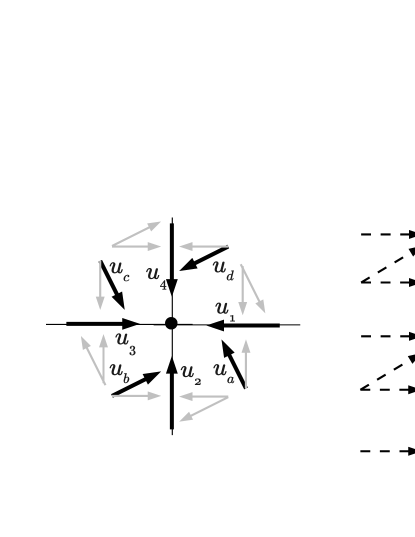
Fixing the gauge does not alter the type or the number of solutions found for the beliefs (which is the physically meaningful quantity, not the fields or messages). However, it can help gaining some more convergence in single instances, and furthermore, becomes necessary to make a correct population dynamics representation of the average case. We decided to fix the gauge by setting to zero one of the fields acting over spins in the plaquette-to-link message , as shown in Fig. 14. Furthermore, since all the bold faced fields in this figure participate in each other equations in a linear way, we solved the set of linear equations in each message passing step, therefore moving all these fields in a consistent way towards agreementDominguez et al. (2011).
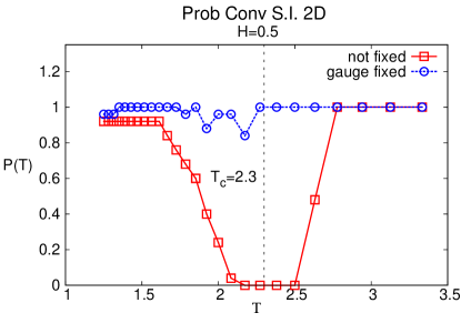
This mixed strategy of fixing the gauge and a consistent updating of all linearly dependent fields showed to improve the convergence of the GBP in the 2D Edwards Anderson modelDominguez et al. (2011). In Fig. 15 we show that this is also the case in the random field Ising model. Most of the convergence problem appearing near the transition line from para to long range ordered phase disappears if the GBP is implemented with these two prescriptions. However, the convergence problems appearing within the long range ordered phase, did not disappear, and a growing island of non convergence still exists for low temperatures and fields, as discussed in the article.
References
- C. De Dominicis et al. (1995) C. De Dominicis, H. Orland, and T. Temesvari, J. Phys. I France 5, 987 (1995).
- Mézard and Monasson (1994) M. Mézard and R. Monasson, Phys. Rev. B 50, 7199 (1994).
- Brézin and De Dominicis (2001) E. Brézin and C. De Dominicis, The European Physical Journal B 19, 467 (2001).
- de Almeida and Bruinsma (1987) J. R. L. de Almeida and R. Bruinsma, Phys. Rev. B 35, 7267 (1987).
- Pastor et al. (2002) A. A. Pastor, V. Dobrosavljević, and M. L. Horbach, Phys. Rev. B 66, 014413 (2002).
- Fytas and Martín-Mayor (2013) N. G. Fytas and V. Martín-Mayor, Phys. Rev. Lett. 110, 227201 (2013).
- Picco and Sourlas (2014) M. Picco and N. Sourlas, J. Stat. Mech.: Theor. Exp. 2014, P03019 (2014).
- Krzakala et al. (2010) F. Krzakala, F. Ricci-Tersenghi, and L. Zdeborová, Phys. Rev. Lett. 104, 207208 (2010).
- Krzakala et al. (2011) F. Krzakala, F. Ricci-Tersenghi, D. Sherrington, and L. Zdeborová, J. of Physics A 44, 042003 (2011).
- Imry and Ma (1975) Y. Imry and S.-k. Ma, Phys. Rev. Lett. 35, 1399 (1975).
- Aharony et al. (1976) A. Aharony, Y. Imry, and S.-k. Ma, Phys. Rev. Lett. 37, 1364 (1976).
- Domínguez et al. (2012) E. Domínguez, A. Lage-Castellanos, and R. Mulet, Rev. Cub. Fis. 29, 14 (2012).
- Mézard and Parisi (2001) M. Mézard and G. Parisi, Eur. Phys. J. B 20, 217 (2001).
- Mézard and Parisi (2003) M. Mézard and G. Parisi, J. Stat. Phys. 111, 1 (2003).
- Viana and Bray (1985) L. Viana and A. J. Bray, J. Phys. C 18, 3037 (1985).
- Mezard et al. (2002) M. Mezard, G. Parisi, and R. Zecchina, Science 297, 812 (2002).
- Mézard and Zecchina (2002) M. Mézard and R. Zecchina, Phys. Rev. E 66, 056126 (2002).
- Mulet et al. (2002) R. Mulet, A. Pagnani, M. Weigt, and R. Zecchina, Phys. Rev. Lett. 89, 268701 (2002).
- Pearl (1988) J. Pearl, Probabilistic Reasoning in Intelligent Systems: Networks of Plausible Inference (Morgan Kaufmann, San Fransico, CA, 1988).
- Kabashima and Saad (1998) Y. Kabashima and D. Saad, Europhys. Lett. 44, 668 (1998).
- Montanari and Rizzo (2005) A. Montanari and T. Rizzo, J. Stat. Mech.: Theor. Exp. 2005, P10011 (2005).
- Chertkov and Chernyak (2006a) M. Chertkov and V. Y. Chernyak, Phys. Rev. E 73, 065102 (2006a).
- Chertkov and Chernyak (2006b) M. Chertkov and V. Y. Chernyak, J. Stat. Mech.: Theor. Exp. 2006, P06009 (2006b).
- Mooij and Kappen (2007) J. M. Mooij and H. J. Kappen, J. Mach. Learn. Res. 8, 1113 (2007).
- Gomez et al. (2010) V. Gomez, H. J. Kappen, and M. Chertkov, J. Mach. Learn. Res. 11, 1273 (2010).
- Jing-Qing Xiao (2011) H. Z. Jing-Qing Xiao, J. Phys. A: Math. Theor. 44, 425001 (2011).
- Haijun Zhou and Bi (2011) J.-Q. X. Haijun Zhou, Chuang Wang and Z. Bi, J. Stat. Mech.: Theor. Exper. 44, L12001 (2011).
- Haijun Zhou (2013) C. W. Haijun Zhou, Journal of Statistical Physics 148, 513 (2013).
- Yedidia et al. (2005a) J. Yedidia, W. T. Freeman, and Y. Weiss, IT-IEEE 51, 2282 (2005a).
- Kikuchi (1951) R. Kikuchi, Phys. Rev. 81, 988 (1951).
- Rizzo et al. (2010) T. Rizzo, A. Lage-Castellanos, R. Mulet, and F. Ricci-Tersenghi, J. Stat. Phys. 139, 375 (2010).
- Lage-Castellanos et al. (2013) A. Lage-Castellanos, R. Mulet, F. Ricci-Tersenghi, and T. Rizzo, J. Phys. A: Math. Theor. 46, 135001 (2013).
- Dominguez et al. (2011) E. Dominguez, A. Lage-Castellanos, R. Mulet, F. Ricci-Tersenghi, and T. Rizzo, J. Stat. Mech. 2011, P12007 (2011).
- Lage-Castellanos et al. (2014) A. Lage-Castellanos, R. Mulet, and F. Ricci-Tersenghi, EPL (Europhysics Letters) 107, 57011 (2014).
- Parisi et al. (1987) G. Parisi, M. Mézard, and M. Virasoro, Spin Glass Theory and Beyond (World Scientific, Singapore, 1987).
- Yedidia et al. (2005b) J. Yedidia, W. T. Freeman, and Y. Weiss, IEEE T. Inform. Theory 51, 2282 (2005b).
- Pelizzola (2005) A. Pelizzola, J. Phys. A 38, R309 (2005).
- Lage-Castellanos et al. (2011) A. Lage-Castellanos, R. Mulet, F. Ricci-Tersenghi, and T. Rizzo, Phys. Rev. E 84, 046706 (2011).
- Bricmont and Kupiainen (1987) J. Bricmont and A. Kupiainen, Phys. Rev. Lett. 59, 1829 (1987).
- Parisi and Dotsenko (1992) G. Parisi and V. Dotsenko, Journal of Physics A: Mathematical and General 25, 3143 (1992).
- Newman and Barkema (1996) M. Newman and G. Barkema, Phys. Rev. E 53, 393 (1996).
- Middleton and Fisher (2002) A. Middleton and D. Fisher, Phys. Rev. B 65, 134411 (2002).
- Parisi, G. et al. (1999) Parisi, G., Ricci-Tersenghi, F., and Ruiz-Lorenzo, J. J., Eur. Phys. J. B 11, 317 (1999).
- Monasson (1998) R. Monasson, J. Phys. A 31, 513 (1998).
- Kabashima (2005) Y. Kabashima, J. Phys. Soc. Jpn. 74, 2133 (2005).