Stochastic Wilson-Cowan models of neuronal network dynamics with memory and delay
Abstract
We consider a simple Markovian class of the stochastic Wilson-Cowan type models of neuronal network dynamics, which incorporates stochastic delay caused by the existence of a refractory period of neurons. From the point of view of the dynamics of the individual elements, we are dealing with a network of non-Markovian stochastic two-state oscillators with memory which are coupled globally in a mean-field fashion. This interrelation of a higher-dimensional Markovian and lower-dimensional non-Markovian dynamics is discussed in its relevance to the general problem of the network dynamics of complex elements possessing memory. The simplest model of this class is provided by a three-state Markovian neuron with one refractory state, which causes firing delay with an exponentially decaying memory within the two-state reduced model. This basic model is used to study critical avalanche dynamics (the noise sustained criticality) in a balanced feedforward network consisting of the excitatory and inhibitory neurons. Such avalanches emerge due to the network size dependent noise (mesoscopic noise). Numerical simulations reveal an intermediate power law in the distribution of avalanche sizes with the critical exponent around . We show that this power law is robust upon a variation of the refractory time over several orders of magnitude. However, the avalanche time distribution is biexponential. It does not reflect any genuine power law dependence.
pacs:
05.40.-a,87.19.lc,87.19.lj,87.19.ll1 Introduction
Network complexity pervades biology and medicine [1], and the human organism can be considered as an integrated complex network of different physiological systems [2] such as circulatory and respiratory systems, visual system, digestive and endocrine systems, etc., which are coordinated by autonomic and central nervous systems including the brain. The dynamics of the sleep-wake transitions during the sleep of humans and other mammals [3, 4, 5] presents one of important examples of such complex dynamics. In turn, functioning of the human brain presents is essence a network activity of the coupled and interrelated neurons surrounded by glia cells. The immense complexity of this subject matter [6] does not exclude, but rather invites thinking in terms of simple physical modeling approaches, see e.g. in Ref. [3], since even very simple physical models can display very complex behavior. The models of critical dynamical phenomena such as self-organized criticality (SOC) [1, 7, 8] are especially important in this respect [4, 5]. Physical modeling can help to discriminate the physical and biological complexity from the complexity of mental processes, the “form within” [6], which is mediated but not determined in fine features by the background physical processes. The recently discovered complexity of the critical brain dynamics [9, 10, 11] in essence does not have anything in common with the complexity of mental processes as it is already displayed by organotypic networks of neurons formed by cortical slices on a multi-electrode array [9]. Such physical complexity is in essence the complexity of crude matter that got self-organized following the physical laws. It thus belongs to statistical physics or system biophysics. Physical models such as SOC are especially important and helpful here.
The Wilson and Cowan model [12] presents one of the well-established models of neuronal network dynamics [13]. It incorporates individual elements in a simplest possible fashion as two-state stochastic oscillators with one quiescent state and one excited state, and random transitions between these two states which are influenced by the mutual coupling among the network elements. The model has been introduced in the deterministic limit of huge many coupled elements in complete neglect of the intrinsic mesoscopic noise and became immensely popular with the years [13], being used e.g. to describe neuronal oscillations in visual cortex within a mean-field approximation [1, 14]. Recently, the previously neglected mesoscopic noise effects were incorporated in this model for a finite-size network [15, 16]. Such a noise has been shown to be very important, in particular, for the occurrence of the critical avalanche dynamics [15] absent in the deterministic Wilson-Cowan model and also for the emergence of oscillatory noisy dynamics [16]. At the first glance, such a noisy dynamics can look like a chaotic deterministic one. Deterministic chaos influenced by the noise can also be a natural feature of a higher-dimensional dynamics, beyond the original two-dimensional Wilson-Cowan mean field model. Indeed, deterministic chaos has been found in the brain dynamics some time ago [17, 1]. However, it cannot be described within the memoryless Wilson-Cowan model because the minimal dimension for chaos is three [18].
Stochastic mesoscopic noise effects due to a finite number of elements in finite size systems attract substantial attention over several decades, especially with respect to chemical reactions on the mesoscale [19, 20], being especially pertinent to the physico-chemical processes in living cells [21]. In particular, such intrinsic noise can cause and optimize spontaneous spiking (coherence resonance [22, 23]) in the excitable clusters of ionic channels in cell membranes, which are globally coupled through the common membrane potential, or the response of such systems to periodic external signals (stochastic resonance [24]) within a stochastic Hodgkin-Huxley model [25]. Finite-size networks of globally coupled bistable stochastic oscillators were also considered without relation to the Wilson-Cowan model [26, 27], including non-Markovian memory effects [28, 29, 23, 30, 31].
In this paper, we consider a class of higher-dimensional generalizations of the stochastic Wilson-Cowan model aimed to incorporate non-Markovian memory effects in the dynamics of individual neurons. Such effects are caused by the existence of a refractory period or inactivated state from which the neuron cannot be excited immediately. First, we discuss a general class of such models. Then, we apply the simplest two-state non-Markovian model of this class, embedded as a three-state Markovian model with one inactivated state, to study a critical avalanche dynamics in a balanced network of the excitatory and inhibitory neurons within a mean-field approximation. Here, we restrict ourselves to the simplest example of a fully connected network with all-to-all coupling of its elements. In particular, we derive the power law exponents characterizing the critical self-organized dynamics of the network from the precise numerical simulations done with the dynamic Monte Carlo, or Gillespie algorithm. We also compare these results with similar results obtained within approximate stochastic Langevin dynamics, or, equivalently, within a diffusional approximation to the discrete state dynamics. Here, we reveal a profound difference.
2 The model and theory
2.1 Stochastic models of single neurons

Let us depart from the Markovian model of a neuron possessing one activated or excited state “a”, and a quiescent state “q”, see Fig. 1, a. The excitation of the neuron occurs with the rate , where is a rate constant and is a dimensionless transfer function which depends on the states of the other neurons, and will be discussed below. Let us assume for a while that is not explicitely time dependent. From the point of view of the theory of continuous time random walks (CTRWs) or renewal processes [32, 33], such a two state neuron can be completely characterized by the residence time distributions (RTDs) in its two states, , and , correspondingly (assuming that no correlations between the residence time intervals is present – the renewal or semi-Markovian assumption). RTDs define completely the trajectory realizations of such a renewal process. In the Markovian case, the RTDs are strictly exponential, , and , where we denoted . Then, such a trajectory description corresponds to the Markovian balance or master equations for the probabilities to populate the states “a” and “q”, and , correspondingly. Due to the probability conservation, ,
| (1) |
The memory effect due to a delay of a new excitation event after the neuron comes into the quiescent state, or the existence of some refractory period , can be captured within the trajectory description by a non-exponential RTD . This transforms the corresponding master equation into a generalized master equation (GME) with memory, where the term is replaced by , with a memory kernel . Here, is the starting time, , if not a different one is explicitely stated. Hence, Eq. (1) is replaced by
| (2) |
In the CTRW theory it is well-known how the memory kernel and the residence time distribution are related [33, 34] (see also Appendix of [35]). Namely, their Laplace-transforms [denoted as , for any function ] are related as
| (3) |
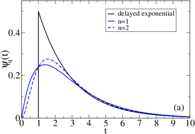
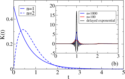
In neurosciences, a delayed exponential, or delayed Poissonian model is popular [36]. It is featured by the absolute refractory period , i.e. , for , and the exponential distribution, , for , see in Fig. 2. This model corresponds to , and the memory kernel . The numerical inverse Laplace transform of this memory kernel is depicted in the inset of Fig. 2, b. Notice that it does not correspond to the memory kernel , which would correspond to the master equation with the deterministic delay [37]
| (4) |
However, this memory kernel is strongly peaked at , and can thus be approximated, with , which is the inverse mean time of the delayed Poissonian distribution . In the corresponding Markovian approximation, Eq. (1) is restored with a renormalized transfer function,
| (5) |
This is the simplest way to account for the delay effects. Obviously, any delay should suppress excitability within this approximation, because . However, suppression of the excitability of the inhibitory neurons may enhance the excitability of the whole network consisting of both excitatory and inhibitory neurons. Hence, possible effects are generally nontrivial even in this approximation. Moreover, Eq. (5) makes it immediately clear that the delay effects are generally expected to be very substantial for .
2.1.1 The simplest non-Markovian model and its Markovian embedding.
It is well-known that in many cases non-Markovian CTRW dynamics can be embedded as some Markovian dynamics in a higher-dimensional, possibly infinite dimensional space [38]. Given a non-trivial form of the memory kernel for the delayed exponential distribution of the quiescent times, we can ask the question: What is the simplest non-Markovian model and the corresponding Markovian embedding to account for the memory effects? From the point of view of GME, it is , i.e. an exponentially decaying memory kernel. The corresponding memory kernel with , and corresponds to , which is the time convolution of two exponential distributions, , and . It corresponds to a compound state “” in Fig. 1, b. Indeed, the Laplace transform of the corresponding compound distribution is just the product of the Laplace-transforms of two exponential distributions, i.e., . By Eq. (3) it corresponds precisely to the stated exponential memory kernel. The corresponding has a maximum at the most probable time interval , see Fig. 2, a, reflecting the most probable stochastic time delay. This simplest non-Markovian model with memory allows, however, for a very simple Markovian embedding by introduction of an intermediated refractory state “i” shown in Fig. 1, b, with the population probability and the exponential RTD given above. It has the mean refractory time , and the relative standard deviation, or the coefficient of variation, . Using the conservation law, , the corresponding master equations can be written either as
| (6) |
or as
| (7a) | |||||
| (7b) | |||||
From (7b) follows
| (8) |
After substitution of this equation into (7a) one obtains indeed Eq. (2) with the discussed exponential memory kernel provided that . The latter condition is natural because every sojourn in the compound quiescent state “” starts from the substate “i” (resetting memory of this neuron to zero), and is the probability of the compound quiescent state within the two-state non-Markovian reduction of the three-state Markovian problem. Here, one can also see the origin of a profound problem with the description of the whole network dynamics of interacting non-Markovian renewal elements as a hyper-dimensional renewal process. Obviously, the behavior of the whole network cannot be considered as a renewal process, because after each and every de-excitation event only one element is reset. Then it starts with zero memory, while all others keep their memory until they are reset. Hence, any Gillespie type simulation of the whole network of interacting non-Markovian elements must account for the “age” of each network element separately. Markovian embedding allows to circumvent this problem and dramatically accelerate simulations within the mean-field approximation, see below.
The considered three-state Markovian cyclic model presents one of the fundamental kinetic models in biophysics. It provides, in particular, a paradigm for non-equilibrium steady state cycling. For example, the cyclic kinetics of an enzyme , which binds a substrate molecule , converts it to a product , and releases it afterwards can be represented as a three-state cycle, . This model was used e.g. in Ref. [29] for an excitable unit. Furthermore, three-state non-Markovian models can be used with a non-exponential distribution . For example, if to use the deterministically delayed , and exponential within the three-state cyclic model, then one obtains the delayed exponential distribution within the two-state reduced model, which was discussed above. In addition, can also be non-exponential. For in the excited state of the three-state non-Markovian model, one obtains the model used in Refs. [28, 29].
2.1.2 Markovian embedding with many substates.
One can also introduce many delayed substates as shown in Fig. 1, c. Within the three-state non-Markovian model this can be considered as having one delayed state “i” characterized by the special Erlangian distribution [32], , with the Laplace-transform reflecting the corresponding multiple convolution. Such a non-Markovian three-state model has been considered in [30], and a non-Markovian two-state model with the Erlangian distribution of the quiescent times has been studied in [31]. The compound quiescent state corresponding to the model in [30] is characterized by . The mean delay time is the same for any , and the coefficient of variation becomes ever smaller with increasing , , i.e. the distribution of the refractory times becomes ever more sharpened. The Laplace-transformed memory kernel is . Some corresponding and are shown in Fig. 2. Already for , the memory kernel starts to show a peaked structure. Notice that in the limit , the above delayed exponential (or Poissonian) model immediately follows with . For any , the inverse mean time in the quiescent state is given by with in (5). Increasing yields an ever better approximation for the delayed Poissonian model. However, it can be considered as a useful model in itself. The corresponding Markovian embedding master equation reads (with excluded by the probability conservation law):
| (9) |
with, , for , initially. With a different initial condition, the corresponding GME obtained upon projection of the multi-dimensional dynamics onto the subspace of and variables will contain a dependence on this initial condition in the subspace of hidden Markovian variables. On the level of non-Markovian dynamics this can be accounted for by a different choice of the residence time distribution for the first sojourn in the quiescent state. It depends on how long this state has been populated before the dynamics started [32]. The GME (2), (3) corresponds to the particular choice, .
We mention in passing also that it is straightforward to consider a power-law distributed delay, both within a semi-Markovian model and within an approximate finite-dimensional Markovian embedding. Also a stochastic model for bursting neurons can be introduced immediately. We shall not, however, consider these possibilities in the present work.
2.2 Network of neurons within the mean field dynamics
Following Wilson and Cowan, we consider a network of excitatory and inhibitory neurons, with the probabilities of neurons to be in their excited states and , correspondingly. The neuron can influence the neuron and possibly itself (), by excitation, or inhibition with the coupling constants, , for the excitatory neuron , and , , for the inhibitory neuron . The absolute value of the coupling constant reflects the synaptic strength. Each excitatory neuron thus obtains an averaged input , and the inhibitory neuron receives the input , where and , etc. is the number of inputs which the th neuron obtains from the excitatory and inhibitory neurons, correspondingly. The constants and serve to fix the spontaneous spiking rates, , , in the absence of coupling, . Coupling can either enhance, or suppress these rates. Phenomenologically, this is accounted for by the transfer function , which we assume to be the same for all neurons. Some common biophysically motivated popular choices of the transfer function are
| (10) |
where is the Heaviside step function, and
| (11) |
Both are bounded as . Evidently, this is a very rich model even for the simplest two-state model of neurons, in the absence of memory effects. The simplest further approximation to describe the collective dynamics of neurons is to invoke the mean field approximation [14]. It is equivalent to assuming that all the coupling constants like , etc., thresholds , etc., and rates , , are equal within a subpopulation, , , , or , etc. Furthermore, one can introduce the occupation numbers of the excited neurons in each population, , and , and consider the dynamics of these variables. They present the fractions of neurons which are excited.
We restrict our treatment in the rest of this paper to the simplest two state non-Markovian model within the three state Markovian embedding and introduce the occupation numbers of neurons, , and , in the corresponding delayed states. Then, in the deterministic limit , one obtains a 4-dimensional nonlinear dynamics,
| (12) |
Notice that unlike the original two-dimensional mean-field Wilson-Cowan dynamics in the deterministic limit, the considered 4-dimensional dynamics can in principle be chaotic, for some parameters (which remains an open question). Dynamical chaos might emerge already when only one sort of neurons, e.g. inhibitory neurons, exhibits delayed dynamics, since the minimal dimension for nonlinear chaotic dynamics is three. Then, in the macroscopic deterministic limit,
| (13) |
However, we shall not investigate the possibility of a deterministic chaos emerging due to a delay within the minimal extensions of the Wilson-Cowan model in the present work, but rather focus on the mesoscopic intrinsic noise effects caused by finite and . Then, the occupational numbers are random variables (at any fixed time ).
2.2.1 Langevin dynamics.
For a very large number of neurons, one can account for the mesoscopic noise effect within the Langevin dynamics, or the diffusional approximation of the discrete state birth-and-death process describing the evolution of the network. This procedure is standard, by analogy with the stochastic theory of chemical reactions [20]. Since we have only direct “reactions” like , , , for two type of neurons, one must introduce six variables and six independent zero-mean white Gaussian noise sources , . Stochastic dynamics is, however, effectively 4-dimensional because of two probability conservation laws, which allow to exclude two variables out of six:
| (14) |
In the limit , the deterministic description in Eq. (2.2) is restored. The noise is multiplicative and the Langevin equations must be Ito-interpreted, as it is always the case if the Langevin dynamics results from the standard diffusional approximation to a birth-and-death process, or chemical master equation [20]. Notice that such a Langevin stochastic description can become problematic, if any of the variables becomes temporally zero or one. Even if some of the noise terms do vanish at the boundaries, where there corresponding rates vanish, the others do not, when a particular boundary is hit. Hence, the occupational numbers can in principle become temporally negative, or larger than one. This unphysical feature is produced by the standard diffusional approximation. However, this problem can be fixed in the numerical simulations by introduction of the corresponding reflecting boundaries and taking sufficiently small integration time steps, as done e.g. in Ref. [25, 41] for stochastic Hodgkin-Huxley equations.
2.3 Exact stochastic simulations.
| Transition | Rate | |
|---|---|---|
| 1 | ||
| 2 | ||
| 3 | ||
| 4 | ||
| 5 | ||
| 6 |
Within the mean-field approximation of Markovian dynamics, it suffices to count the numbers of neurons in the corresponding activated, and , and refractory, and states. Then, we are dealing with a random walk on a 4-dimensional lattice with the discrete variables , and taking values in the range from zero to , and the variables and in the range from zero to , so that also and . From the site six different transitions are possible. They are enlisted in Table 1 with the corresponding transition rates. The master equation governing this birth-and-death process can be readily written. However, it is bulky and not very insightful. For this reason, it is not presented here. The corresponding stochastic process can be easily simulated with the dynamical Monte Carlo or Gillespie algorithm [19], which is exact. Namely, on each step one draws two random numbers. The first one, , is drawn from the exponential distribution characterized by the total rate . It gives a random time interval at which the network state is updated. Given a uniformly distributed random variable , , . Then, one of the transitions in Table 1 is chosen in accordance with its probability . For this, one generates a uniformly distributed random variable bounded as . If , then the first transition is chosen. If , then the second transition is chosen, etc., i.e. in accordance with the length of the corresponding interval , .
Notice that an attempt to generalize this scheme towards a non-Markovian renewal walk on a 4-dimensional lattice to account for the memory in the inactivated state is logically inconsistent because in such a case accomplishing each step would mean reset, or renewal of all neurons, and not the only one which actually makes transition. However, each non-Markovian element has its individual memory. In a direct simulation of the network of non-Markovian elements one must therefore consider them individually, even within the mean-field approximation. Then, one has to consider CTRW on a hyper-dimensional lattice of huge dimensionality, which will dramatically slow down simulations imposing computational restrictions on the maximal size of the network. Of course, beyond the mean field approximation one must also simulate each element separately. Here, a direct semi-Markovian approach can be preferred. In this work, we restrict ourselves to the mean-field dynamics within the Markovian embedding framework, which allows for exact simulations of very large networks within a reasonable computational time.
3 Results and Discussion
3.1 Oscillatory dynamics of neuronal network
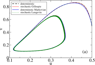
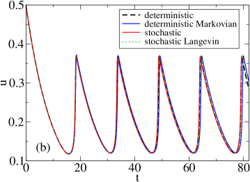
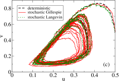
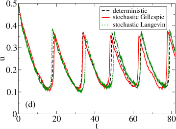
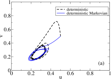
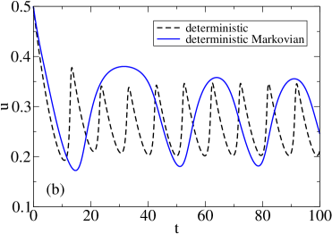
First, we test our stochastic simulations done with XPPAUT [42] against nonlinear deterministic dynamics for a very large network size with and . For this, departing from the parameter set in Ref. [16] (the case of without delay) we use a set of parameters, where an oscillatory dynamics emerges: , , , , , , , , , , , , and the transfer function in Eq. (11). Time is in milliseconds and the rate constants are in inverse milliseconds. The difference is barely detectable in Fig. 3, a, b, where we present the results of stochastic simulations done both with the exact Gillespie algorithm and within the approximate Langevin dynamics. However, stochastic effects become immediately seen in Fig. 3, c, d, where we reduced the number of neurons to and . We also compare in Fig. 3, a, b, the results for the considered dynamics and its two-variable Markovian approximation given by the standard Wilson-Cowan model in which, however, the transfer functions are renormalized in accordance with Eq. (5), where the parameter is replaced by and , correspondingly. The deviations are visible, but small. However, the differences become very pronounced for small corresponding to the mean refractory period of 10 msec. Then, the Markovian approximation fails completely, see in Fig. 4, especially in part (b), revealing that neither the form of the oscillations, not their period are reproduced even approximately. Especially remarkable is that contrary to intuition the increase of the refractory period of a single neuron does not increase the period of oscillations, as the Markovian approximation predicts, but rather makes it smaller – the tendency is opposite! Therefore, non-Markovian memory effects generally do matter and one should take such effects seriously into account. With a small further decrease of to with the oscillations are terminated by a supercritical Hopf bifurcation (not shown). Interestingly, Markovian approximation also predicts such a termination, but at a slightly larger critical value with critical . This makes clear that the phase transitions between the quiescent network and the network undergoing synchronized oscillations are possible with respect to the length of the refractory period used as a control parameter.
3.2 Noise-induced critical avalanche dynamics
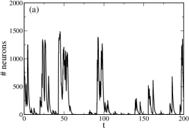
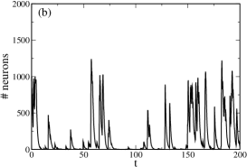
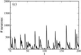
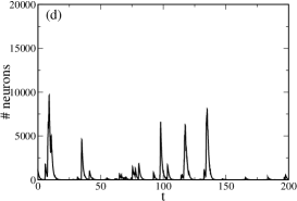
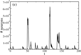
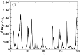
In the remainder, we investigate the influence of memory effects on the avalanche dynamics. As it has been shown in [15], in order to have avalanche dynamics the excitatory and inhibitory processes should be nearly balanced, and the network should have a so-called feedforward structure. Then, one can achieve a sort of self-organized critical (SOC) state [7, 8] sustained due to intrinsic mesoscopic fluctuations. Very different from other SOC models, here fluctuations play a major role and in the deterministic limit avalanches disappear, i.e. they are of mesoscopic nature. The nullclines of 2d deterministic dynamics in the absence of memory effects, and , should cross at a very small angle in the plane, so that fluctuations can produce large amplitude outbursts of the and variables moving synchronously but randomly, i.e. the subpopulations of excitatory and inhibitory neurons are synchronized exhibiting stochastic dynamics at the same time [15]. In the same spirit, we choose , , , , so that , and overall excitation slightly dominates over inhibition. Furthermore, we choose , and the transfer function in Eq. (10), as in Ref. [15]. The rates , and the number of neurons were varied. Large corresponds to a small refractory time of msec, whereas corresponds to a profound delay with msec, so that the individual spiking rate of neurons cannot exceed 100 Hz being limited by the refractory period. Typical avalanche dynamics is shown in Fig. 5 for with , and (a) , (b) , (c) . Furthermore, in Fig. 5, d, e, f, we show the influence of an increasing number of neurons on the avalanche dynamics. The following tendencies are clear. First, the increase of refractory period reduces the maximal amount of neurons involved in spiking, from about 76% in Fig. 5, a to 58.5% in Fig. 5, c. Such a tendency is already expected from the renormalization of the transfer function in the Markovian approximation, cf . Eq. (5). However, this tendency is in fact much weaker since in the part (c), and the renormalization argumentation would predict almost complete suppression of avalanches for such a delay. Even more astonishing is that avalanches still did not vanish even for a very large , see Fig. 5, f. This is very different from the oscillatory dynamics of a network of the same size, cf. Fig. 3, a, and b, which is practically deterministic. Of course, with increasing network size, the relative amplitude of avalanches becomes ever smaller, and there also emerges a minimal number of neurons excited, i.e. the network activity never goes down to zero. However, this is also so in the real neuronal dynamics. Such a dominance of mesoscopic fluctuations in a system of millions elements with a special (feedforward) structure of coupling is really astonishing. This is a feature of some critical state, as we know from statistical physics.
To statistically characterize the avalanche size distribution and their duration we proceed in accordance with the procedure outlined in Ref. [15]. It reflects, in part, also the experimental procedure [10]. Namely, we first discretize the time series with a time bin of the size , which corresponds to the averaged interspike time distance in a particular simulation. Then, an avalanche is defined by its start, when the spiking activity crosses some threshold level , and its end, when the network activity drops to () or below after some time, which defines the avalanche duration. The size is defined as the sum of the number of neurons active in each time bin during the avalanche. It is also defined experimentally in such a way. In essence, the size of an avalanche is the integral of the network activity in Fig. 5 over the time during each avalanche period divided by the time bin width. Of course, as also in experiments the critical exponents discussed below depend both on the time bin width and on the basal level of neuronal activity . However, this dependence is weak for a truly critical dynamics. By doing statistical analysis, we first find the survival probability , or, equivalently, the cumulative probability from the numerical data. Then, the distribution density follows as .
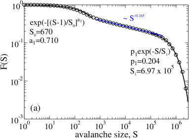
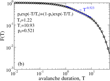
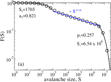
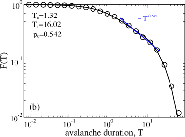
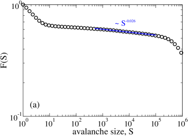
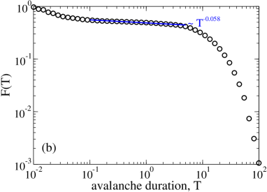
Let us start from the case without any time delay, . The survival probability for the avalanche size distribution is shown in Fig. 6,a, for the time bin and . It shows three characteristic features: (1) an initial Weibull distribution, , with and ; (2) an intermediate power law , with , and (3) an exponential tail with and . The size distribution is, therefore, initially approximately a power law with negative exponent , followed by a power law with negative exponent . The latter one extends over approximately two size decades and ends with an exponential tail characterized by a cutoff size, . The corresponding survival probability for the avalanche durations is shown in Fig. 6, b. It can be well fitted by a sum of two exponentials,
| (15) |
However, it also seems to display an intermediate power law over about one time decade, from 1 to 10 ms, with the power exponent , and the cutoff time ms. Hence, the probability distribution also appears to reflect an intermediate power law with . Interestingly, the duration of avalanches in experiments with organotypic cortical neuronal systems has a similar cutoff time of about 10-20 ms, with a maximal avalanche duration of about 40-80 ms, which is restricted by the period of oscillations [10]. The intermediate power law also extends over about one time decade in the experiments. However, the experimental power law exponent is different, . It should be mentioned in this respect that the time bin in the experiments is also very different, ms. One electrode measures in experiments a contribution of many neurons. In fact, coarse graining over some unknown should be done. The experimental size exponent is also different, . It is not, however, the goal of this paper to provide a model fully consistent with the experimental observations, which are subject of ongoing research work and some controversy in the literature [43]. In this respect, a bi-exponential dependence can be perceived as a power law over one intermediate time decade, as our fit also shows.
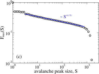
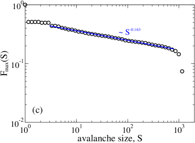
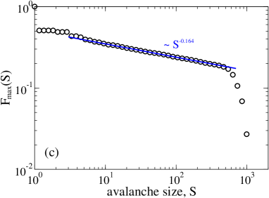
As an additional characteristics of the avalanches size, one can also consider the maximal number of neurons activated at once during an avalanche, or the avalanche peak with a distribution density . The corresponding survival probability, , also exhibits a power law, , with , in Fig. 6, c. Hence, , with , which only slightly differs from meaning that the avalanche size is roughly proportional to its peak. However, the cutoff of is super-exponentially sharp, because the maximal number of neurons involved in an avalanche at the same time is restricted by the total number of neurons in the network. Furthermore, reveals a very large portion of avalanches whose peak does not exceed 10, which explains the initial stretched exponential dependence in Fig. 6, a. Strictly speaking, this part of the size distribution (with ) reflects a background or basal noise, where neurons practically do not interact with each other, and there are no avalanches of spontaneously increased activity, which are characterized by a power law distribution.
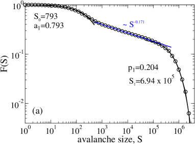
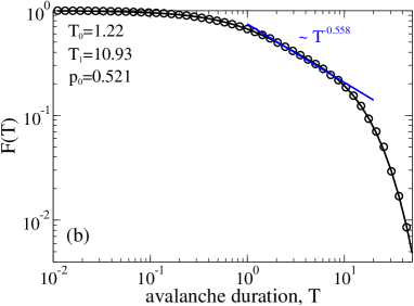
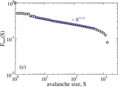
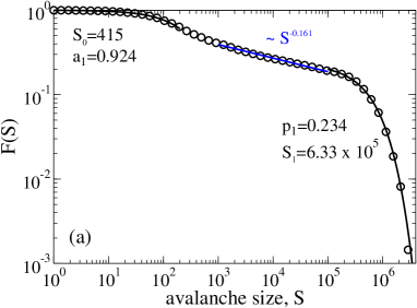
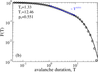
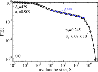
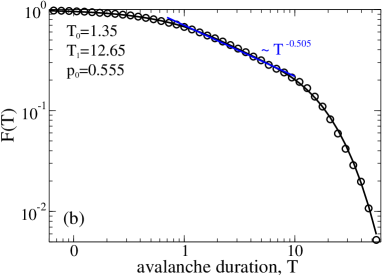
Next, we like to clarify how robust these features are for networks with a time delay. For this, we study the influence of the mean delay time by decreasing the rates from through to in Figs. 7, 8, 9, respectively. The mean delay time increases, accordingly, from through to ms. Even though the parameters of the distributions do change, these changes are not dramatical. In particular, the corresponding critical size exponent changes from (no delay), to , and , respectively. Accordingly, the critical time exponent changes from (no delay) to , , and , respectively. Such changes are not statistically significant, and one cannot detect any systematic tendency upon a variation of . The point is that these exponents are also changed a bit, if we use e.g. , or for the time bin (not shown). They also depend on the threshold . In this respect, if to change from to , the initial stretched exponential part of the size distribution practically disappears. However, there appears an initial power law instead, see in Fig. 10. Remarkably, the intermediate power law exponent remains rather robust. It is changed from in Fig. 7,a to in Fig. 10, a. This is a small variation. Notice, however, that the results in Fig. 10, b in fact reject the hypothesis that there is an intermediate power law in the time distribution of avalanches. First, the power law region changes from larger to smaller times, and also (more important!) the corresponding time exponent changes from in Fig. 7, b to in Fig. 10, b. Clearly, such a strong influence of the choice of on the “power law” exponent makes it clear that this is not a power law. In fact, the time distribution is clearly biexponential.
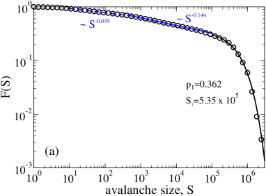
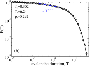
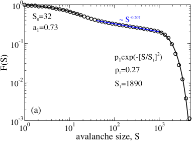
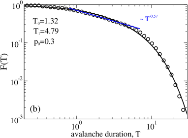
Though plausible until this point, it remains, however, strictly speaking, still not quite clear if is indeed a critical exponent. If true, the extension of the power law domain of the whole size-distribution and the cutoff size should increase with the system size accordingly. Indeed, if we increase the system size tenfold keeping the other parameters the same as in Fig. 9, the power law domain in the size distributions also increases by an order of size magnitude, see in Fig. 11, a. The time cutoff also increases in Fig. 11, b, i.e. the avalanches become longer. Also with decreasing the system size tenfold the power law domain shrinks accordingly in size, see Fig. 12, a, and the avalanches become essentially shorter, as indicated by the decreased cutoff time in Fig. 12, b. Such scaling dependencies on the system size are typical in experiments. From this we can conclude that the size exponent is indeed a critical exponent. However, within the considered model the avalanches do gradually vanish with an increase of the system size. Therefore, the adjective “critical” should be used also with respect to the exponent with some reservations. We consider a rather atypical SOC model, even though the exponent is by chance close to that of the sandpile model [7, 8]. It should also be noticed that the initial distributions of the sizes and times and the tail functional dependencies can be sensitive to both the system size and the choice of the threshold . For example, the size distribution exhibits a Gaussian tail in Fig. 12, a, for a small system size. The intermediate power law in the size distribution is, however, rather robust, with being in the range for the data presented, with the average .
3.2.1 Langevin dynamics of avalanches.
Within the Langevin approximation of the discrete state dynamics, the avalanches look very similar to the ones depicted in Fig. 5. However, their statistics is very different. We performed the corresponding Langevin simulations for the same parameters as in Figs. 7, 10 with the time step taken to be the same as the time bin used to produce the results in Figs. 7, 10. We also used to analyze the data, as in Fig. 10. The results shown in Fig. 13 reveal similar intermediate power laws both in the size and the time distributions yielding , . However, these results differ essentially from the results obtained within the exact dynamic Monte Carlo simulations, compare Fig. 13 with Fig. 10. This indicates that the Gauss-Langevin or diffusional approximation of the genuine discrete state dynamics can deliver incorrect results for the fluctuation-induced avalanche dynamics. This fact makes any analytical theory for the numerical results presented in this work especially challenging. It is almost hopeless to develop such a theory for the discrete state avalanche dynamics within the studied model. Multi-dimensional birth-and-death processes are very difficult for any analytical treatment. Within the Langevin dynamics approximation, or the equivalent multi-dimensional Fokker-Planck equation description an analytical treatment is more feasible. However, such a theory will not help to understand the critical features of the discrete state dynamics, as our numerical results imply.
4 Summary and Conclusions
In this paper, we studied a generalization of the stochastic Wilson-Cowan model of neuronal network dynamics aimed to incorporate a refractory period delay on the level of individual elements. Considered as stochastic bistable elements such model neurons exhibit non-Markovian dynamics with memory, which can be characterized by a non-exponential residence time distribution in the resting state of the neuron (semi-Markovian description), or, alternatively, by the related memory kernel within a generalized master equation description. Such a non-Markovian description generally allows for a Markovian embedding by enlarging the dynamical space upon introduction of new state variables. The simplest two-state non-Markovian model with an exponentially decaying memory kernel can be embedded as a three state cyclic Markovian model, where the refractory period is exponentially distributed. Multi-state Markovian embedding also allows to treat a special Erlangian distribution of the refractory periods, which can be sharply peaked at a characteristic delay time. Moreover, models of bursting neurons and neurons with a power law distributed memory can, in principle, be considered in this generic Markovian embedding setup. The approach of Markovian embedding is especially suitable to treat the mean-field dynamics of the network, which presents a Markovian renewal process in the enlarged space of collective network variables. This is the simplest kind of network, where all the elements are virtually connected in all-to-all fashion. In this respect, the mean field dynamics of a network of non-Markovian renewal elements does not represent a renewal process in the reduced space of non-Markovian collective variables. Then, all the elements must be treated individually, keeping trace of their individual memory. The methodology of Markovian embedding allows to circumvent this problem for the mean-field dynamics.
In the Wilson-Cowan model, two different sorts of interacting neurons are considered, excitatory and inhibitory. We focused on the simplest non-Markovian generalization of this model, where the observed two-state non-Markovian dynamics of a single neuron is embedded as a three state cyclic Markovian process. The corresponding nonlinear mean-field dynamics is four dimensional. It has two dimensions more than in the original model. Moreover, it is stochastic and includes mesoscopic fluctuations due to a finite network size. For a sufficiently large system size, stochastic dynamics can be described within a Langevin equation approximation following the so-called chemical Langevin equation approach, with the noise terms vanishing in the deterministic limit of infinite size. We also exactly simulated the underlying dynamics as a continuous time Markovian random walk on a four-dimensional lattice using the well-known dynamical Monte Carlo (Gillespie) algorithm. The results of both stochastic approaches agree well with the deterministic dynamics within an oscillatory regime for a very large number of elements (several millions). Here, we showed that non-Markovian effects can be very essential. In particular, even deterministic dynamics with an exponentially decaying memory in the space of observable variables can be very different from the dynamics obtained within the Markovian approximation utilizing a delay-renormalized transfer function – the simplest approach to account for the delay effects. However, already the simplest approach allows to describe a dynamical phase transition from the silent network to coherent nonlinear oscillations of synchronized neurons upon a change of the delay period. This important feature is absent in the original Wilson-Cowan model.
In more detail, we investigated the avalanche dynamics in a critically balanced network, where the processes of excitation and inhibition nearly compensate each other in the deterministic limit, where no avalanches are possible within the model considered. Mesoscopic noise fluctuations make, however, avalanches possible even in large networks with millions of neurons, where the deterministic description becomes completely inadequate, very differently from the oscillatory dynamics in such large networks. This result goes beyond the results in Ref. [15], where the avalanches cease to exist for already several tens of thousands elements. Even though a large delay should suppress avalanches by a transfer function renormalization if to think within the Markovian approximation, in reality the suppression is much weaker. Moreover, it turns out that the power law characterizing the distribution of avalanche sizes is very robust with respect to variation of both the delay period, and the system size, over several orders of magnitude, as well as the choice of the avalanche threshold. The latter fact proves that this is a real power law originated due to critical dynamics. It is characterized by a power-law exponent around which is similar to the size exponent of the critical sandpile dynamics (though the both models are not really comparable). However, it is different from the critical exponent found in Ref.[15], though for different network parameters. The distribution of the avalanches durations is, however, biexponential. We disproved that it presents a power law within our model, even though it can look like a power law over one time decade, as in experiments. In this respect, experiments [9, 10, 11] seem to reveal a real power law with the critical size exponent because its range extends with the growing system size. However, the experimental power law in the time duration does not show this important property. As a matter of fact, it extends over merely one time decade being restricted by the period of oscillations. Any power law extending over one time or spatial decade can be fitted by a sum of just two exponentials, as we also show in this work for the time distribution. A further research is, therefore, required to clarify the nature of the apparent power law feature in the avalanche time distribution for the observed neuronal avalanches.
Also very important is that the Langevin or diffusional approximation does change the critical exponents of the studied avalanche dynamics. There appears a power law in the time distribution, which is absent in the exact simulations, with the critical Langevin exponent . Also the critical Langevin size exponent is different, . This feature should be kept in mind while doing diffusional approximations in other models of critical dynamics. It may deliver incorrect results even for a large number of elements.
We believe that the results of this work have methodological value and can be extended onto the dynamics of other networks with delay. They can serve also as a basis for further investigations of the role of non-Markovian memory effects in the dynamics of Wilson-Cowan type neuronal networks, including networks of bursting neurons, and networks with nontrivial topology, which we plan to investigate in future.
5 Acknowledgments
Financial support by the Deutsche Forschungsgemeinschaft, Grant GO 2052/1-2 is gratefully acknowledged.
References
References
- [1] R. Sole and B. Goodwin, Signs of Life: How Complexity Pervades Biology (Basic Books, New York, 2000).
- [2] A. Bashan, R. P. Bartsch, J. W. Kantelhardt, S. Havlin, and P. Ch. Ivanov, Nature Commun. 3, 702 (2012).
- [3] C-C. Lo, L.A.N. Amaral, S. Havlin, P. Ch. Ivanov, T. Penzel, J.-H. Peter, and H. E. Stanley, Europhys. Lett. 57, 625 (2002).
- [4] C-C. Lo, T. Chou, T. Penzel, T. Scammell, R. E. Strecker, H. E. Stanley, and P. Ch. Ivanov, Proc. Natl. Acad. Sci. 101, 17545 (2004).
- [5] C-C. Lo, R. P. Bartsch, and Ch. Ivanov, EPL 102, 10008 (2013).
- [6] K. H. Pribram, The Form Within: My Point of View (Prospecta Press, Westport, 2013).
- [7] P. Bak, C. Tang, and K. Wiesenfeld, Phys. Rev. Lett. 59, 381 (1987).
- [8] J. Kertesz and L. B. Kiss, J. Phys. A: Math. Gen. 23, L433 (1990).
- [9] J. M. Beggs and D. Plenz, J. Neurosci. 23, 11167 (2003).
- [10] D. Plenz, Eur. Phys. J. Special Topics 205 259 (2012).
- [11] J. M. Beggs, Phil. Trans. R. Soc. A 366, 329 (2008).
- [12] H. R. Wilson and J. D. Cowan, Biophys. J. 12, 1 (1972); Kybernetik 13, 55 (1973).
- [13] A. Destexhe and T. J. Sejnowski, Biol. Cybern. 101, 1 (2009).
- [14] H.G. Schuster and P. Wagner, Biol. Cybern. 64, 77 (1990).
- [15] M. Benayon, J. D. Cowan, W. van Drongelen, and E. Wallace, PLoS Comp. Biol. 7, e1000846 (2010).
- [16] E. Wallace, M. Benayon, W. van Drongelen, and J. D. Cowan, PLoS ONE 6, e14804 (2011).
- [17] A. Babloyanz and A. Destexhe, Proc. Natl. Acad. Sci. USA 83, 3513 (1986).
- [18] E. Ott, Chaos in dynamical systems (Cambridge University Press, Cambridge, 1993).
- [19] D. T. Gillespie, J. Comp. Phys. 22, 403 (1976).
- [20] D. T. Gillespie, J. Chem. Phys. 113, 297 (2000).
- [21] R. Phillips, J. Kondev, J. Theriot, and H. G. Garcia, Physical Biology of the Cell, 2nd ed. (Garland Science, London, 2013).
- [22] A. S. Pikovsky and J. Kurths, Phys. Rev. Lett. 78, 775 (1997).
- [23] B. Linder, J. Garcia-Ojalvo, A. Neiman, and L. Schimansky-Geier, Phys. Rep. 392, 321 (2004).
- [24] L. Gammaitoni, P. Hänggi, P. Jung, and F. Marchesoni, Rev. Mod. Phys. 70 223 (1998).
- [25] G. Schmid, I. Goychuk, and P. Hänggi, Europhys. Lett. 56, 22 (2001).
- [26] M. Turalska, M. Lukovic, B. J. West, and P. Grigolini, Phys. Rev. E 80, 021110 (2009).
- [27] I. L. D. Pinto, D. Escaff, U. Harbola, A. Rosas, and K. Lindenberg, Phys. Rev. E 89, 052143 (2014).
- [28] A. Nikitin, Z. Neda, and T. Viscek, Phys. Rev. Lett. 87, 024101 (2001).
- [29] T. Prager, B. Naundorf, L. Schimansky-Geier, Physica A 325, 176 (2003).
- [30] T. Prager, M. Falcke, L. Schimansky-Geier, and M. A. Zaks, Phys. Rev. E 76, 011118 (2007).
- [31] N. Kouvaris, F. Müller, and L. Schimansky-Geier, Phys. Rev. E 82, 061124 (2010).
- [32] D. E. Cox, Renewal Theory (Methuen,London, 1962).
- [33] B. D. Hughes, Random walks and Random Environments, Vols. 1,2 (Clarendon Press, Oxford, 1995).
- [34] V. M. Kenkre, E. W. Montroll, and M. F. Shlesinger, J. Stat. Phys. 9, 45 (1973).
- [35] I. Goychuk, Phys. Rev. E 70, 016109 (2004).
- [36] Ch. Koch, Biophysics of Computation, Information Processing in Single Neurons (Oxford University Press, New York, 1999).
- [37] L. S. Tsimring and A. Pikovsky, Phys. Rev. Lett. 87, 250602 (2001).
- [38] J. W. Haus and K. W. Kehr, Phys. Rep. 150, 263 (1987).
- [39] H. Stehfest, Comm. ACM 13, 47 (1970); H. Stehfest, Comm. ACM 13, 624 (1970)(Erratum).
- [40] I. Goychuk and P. Hänggi, Chem. Phys. 324, 160 (2006).
- [41] I. Goychuk, Commun. Comp. Inf. Sci. 438, 325 (2014).
- [42] B. Ermentrout, Simulating, Analyzing, and Animating Dynamical Systems: a Guide to XPPAUT for Researchers and Students (SIAM, 2002).
- [43] J. Touboul and A. Destexhe, PLoS ONE 5, e8982 (2010).