Approximations and bounds for binary Markov random fields

Abstract

Discrete Markov random fields form a natural class of models to represent images and spatial data sets. The use of such models is, however, hampered by a computationally intractable normalising constant. This makes parameter estimation and a fully Bayesian treatment of discrete Markov random fields difficult. We apply approximation theory for pseudo-Boolean functions to binary Markov random fields and construct approximations and upper and lower bounds for the associated computationally intractable normalising constant. As a by-product of this process we also get a partially ordered Markov model approximation of the binary Markov random field. We present numerical examples with both the pairwise interaction Ising model and with higher-order interaction models, showing the quality of our approximations and bounds. We also present simulation examples and one real data example demonstrating how the approximations and bounds can be applied for parameter estimation and to handle a fully-Bayesian model computationally.

Keywords: Approximate inference; Bayesian analysis; Discrete Markov random fields; Image analysis; Pseudo-Boolean functions; Spatial data; Variable elimination algorithm.

1 Introduction

In statistics in general and perhaps especially in spatial statistics we often find ourselves with distributions known only up to an unknown normalising constant. Calculating this normalising constant typically involves high dimensional summation or integration. This is the case for the class of discrete Markov random fields (MRF). A common situation in spatial statistics is that we have some unobserved latent field $x$ for which we have noisy observations $y$. We model $x$ as an MRF with unknown parameters $\theta$ for which we want to do inference of some kind. If we are Bayesians we could imagine adding a prior for our parameters $\theta$ and studying the posterior distribution $p(\theta|y)$. A frequentist approach could involve finding a maximum likelihood estimator for our parameters. Without the normalising constant, these become non-trivial tasks.

There are a number of techniques that have been proposed to overcome this problem. The normalising constant can be estimated by running a Markov chain Monte Carlo (MCMC) algorithm, which can then be combined with various techniques to produce maximum likelihood estimates, see for instance Geyer and Thompson (1995), Gelman and Meng (1998) and Gu and Zhu (2001). Other approaches take advantage of the fact that exact sampling can be done, see Møller et al. (2006). In the present report however, we focus on the class of deterministic methods, where deterministic in this setting is referring to that repeating the estimation process yields the same estimate. In Reeves and Pettitt (2004) the authors devise a computationally efficient algorithm for handling so called general factorisable models of which MRFs are a common example. This algorithm, which we refer to from here on as the variable elimination algorithm, grants a large computational saving in calculating the normalising constant by exploiting the factorisable structure of the models. For MRFs defined on a lattice this allows for calculation of the normalising constant on lattices with up to around 20 rows for models with first order neighbourhoods. In Friel and Rue (2007) and Friel et al. (2009) the authors construct approximations for larger lattices by doing computations for a number of sub-lattices using the algorithm in Reeves and Pettitt (2004).

The energy function of a binary MRF is an example of a so called pseudo-Boolean function. In general, a pseudo-Boolean function is a function of the following type, $f:\{0,1\}^{n}\rightarrow\mathbb{R}$. A full representation of a pseudo-Boolean function requires $2^{n}$ terms. Finding approximate representations of pseudo-Boolean functions that require fewer coefficients is a well studied field, see Hammer and Holzman (1992) and Grabisch et al. (2000). In Hammer and Rudeanu (1968) the authors show how any pseudo-Boolean function can be expressed as a binary polynomial in $n$ variables. Tjelmeland and Austad (2012) expressed the energy function of MRFs in this manner and by dropping small terms during the variable elimination algorithm constructed an approximate MRF.

Our approach and the main contribution of this paper is to apply and extend approximation theory for pseudo-Boolean function to design an approximate variable elimination algorithm. By approximating the binary polynomial representing the distribution before summing out each variable we get an algorithm less restricted by the dependence structure of the model, thus capable of handling MRFs defined on large lattices and MRFs with larger neighbourhood structures. For the MRF application this approximation defines an approximation to the normalising constant, and as a by-product we also get a partially ordered Markov model (POMM) approximation to the MRF. For the POMM approximation we can calculate the normalising constant and evaluate the likelihood, as well as generate realizations. We also discuss how to modify our approximation strategy to instead get upper and lower bounds for the normalising constant, and how this in turn can be used to construct an interval in which the maximum likelihood estimate must lie. We also discuss another variant of the approach which produces an approximate version of the Viterbi algorithm (Künsch, 2001).

The article has the following layout. In Section 2 we define pseudo-Boolean functions and give a number of approximation theorems for this function class. Thereafter, in Section 3 we introduce binary MRFs and the variable elimination algorithm, and in Section 4 we apply the approximation theorems for pseudo-Boolean functions to define our approximative variable elimination algorithm for binary MRFs. In Section 5 we define a modified variant of the approximate variable elimination algorithm through which we obtain upper and lower bounds for the normalising constant of a binary MRF, and we discuss how to modify the approximation algorithm to obtain an approximate version of the Viterbi algorithm. We briefly discuss some implementational issues in Section 6, and in Section 7 we present simulation and data examples. Finally, in Section 8 we provide closing remarks.

2 Pseudo-Boolean functions

In this section we introduce the class of pseudo-Boolean functions and discuss various aspects of approximating pseudo-Boolean functions partly based on results of Hammer and Holzman (1992) and Grabisch et al. (2000).

2.1 Definition and notation

Let $x=(x_{1},\ldots,x_{n})\in\Omega=\{0,1\}^{n}$ be a vector of binary variables and let $N=\{1,\ldots,n\}$ be the corresponding list of indices. Then for any subset $\Lambda\subseteq N$ we associate an incidence vector $x$ of length $n$ whose $k$th element is $1$ if $k\in\Lambda$ and $0$ otherwise. We refer to an element of $x$, $x_{k}$, as being "on" if it has value $1$ and "off" if it is $0$. A pseudo-Boolean function $f$, of dimension $\mbox{dim}(f)=n$, is a function that associates a real value to each vector, $x\in\{0,1\}^{n}$, i.e $f:\{0,1\}^{n}\rightarrow\mathbb{R}$. Hammer and Rudeanu (1968) showed that any pseudo-Boolean function can be expressed uniquely as a binary polynomial,

$$f(x)=\sum_{\Lambda\subseteq N}\beta^{\Lambda}\prod_{k\in\Lambda}x_{k},$$ (1)

where $\beta^{\Lambda}$ are real coefficients which we refer to as interactions. We define the degree of $f$, $\mbox{deg}(f)$ as the degree of the polynomial. In general the representation of a function in this manner requires $2^{n}$ coefficients. In some cases one or more $\beta^{\Lambda}$ might be zero and in this case a reduced representation of the pseudo-Boolean function can be defined by excluding some or all the terms in the sum in (1) where $\beta^{\Lambda}=0$. Thus we get,

$$f(x)=\sum_{\Lambda\in S}\beta^{\Lambda}\prod_{k\in\Lambda}x_{k},$$ (2)

where $S$ is a set of subsets of $N$ at least containing all $\Lambda\subseteq N$ for which $\beta^{\Lambda}\neq 0$. We then say that $f(x)$ is represented on $S$. Moreover, we say that our representation of $f$ is dense if for all $\Lambda\in S$, all subsets of $\Lambda$ are also included in $S$. The minimal dense representation of $f$ is thereby (2) with,

$$S=\{\lambda\subseteq N:\beta^{\Lambda}\neq 0\text{ for some }\Lambda\supseteq\lambda\}.$$ (3)

Throughout this report we restrict the attention to dense representations of pseudo-Boolean functions.

We also need notation for some subsets of $S$ and $\Omega$. For $\lambda\in S$ we define $S_{\lambda}=\{\Lambda\in S:\lambda\subseteq\Lambda\}$, the set of all interactions that include $\lambda$. For example if $n=3$ and $S=\{\emptyset,\{1\},\{2\},\{3\},\{1,2\},\{1,3\},\{2,3\},\{1,2,3\}\}$, we have $S_{\{1,2\}}=\{\{1,2\},\{1,2,3\}\}$. Equivalently for the set $\Omega$, for $\lambda\in S$ we define $\Omega_{\lambda}=\{x\in\Omega:x_{k}=1,\text{ }\forall k\in\lambda\}$, the set of all states $x$ where $x_{k}$ are on for all $k\in\lambda$. For the same $S$ as above we have for instance $\Omega_{\{1,2\}}=\{(1,1,0),(1,1,1)\}$. We will use also the complements of these two subsets, $S_{\lambda}^{c}=S\setminus S_{\lambda}$ and $\Omega_{\lambda}^{c}=\Omega\setminus\Omega_{\lambda}$. Lastly we define $S_{\lambda}^{0}=\{\Lambda\in S:\lambda\cap\Lambda=\emptyset\}$ and $\Omega_{\lambda}^{0}=\{x\in\Omega:x_{k}=0,\text{ }\forall k\in\lambda\}$. If we think of the sets $S_{\lambda}$ and $\Omega_{\lambda}$ as the sets where $\lambda$ is on, then $S_{\lambda}^{0}$ and $\Omega_{\lambda}^{0}$ are the sets where $\lambda$ is off. Again, using the same example $S$ as above we have for instance $S_{\{1,2\}}^{0}=\{\emptyset,3\}$ and $\Omega_{\{1,2\}}^{0}=\{\{0,0,0\},\{0,0,1\}\}$. Note that in general $S_{\lambda}^{c}\neq S_{\lambda}^{0}$ and equivalently $\Omega_{\lambda}^{c}\neq\Omega_{\lambda}^{0}$.

2.2 Approximating pseudo-Boolean functions

For a general pseudo-Boolean function, the number of possible interactions in our representation grows exponentially with the dimension $n$. It is therefore natural to ask if we can find an approximate representation which requires less memory. We could choose some set $\tilde{S}\subseteq S$ to define our approximation, thus choosing which interactions to retain, $\tilde{S}$, and which to remove, $S\setminus\tilde{S}$. For a given $\tilde{S}$ our interest lies in the best such approximation according to some criteria. We define $A_{\tilde{S}}\{f(x)\}=\tilde{f}(x)=\sum_{\Lambda\in\tilde{S}}\tilde{\beta}^{\Lambda}\prod_{k\in\Lambda}x_{k}$ as the operator which returns the approximation that, for some given approximation set $\tilde{S}$, minimises the error sum of squares (SSE),

$$\mbox{SSE}(f,\tilde{f})=\sum_{x\in\Omega}\left\{f(x)-\tilde{f}(x)\right\}^{2}.$$ (4)

We find the best approximation by taking partial derivatives with respect to $\tilde{\beta}^{\lambda}$ for all $\lambda\in\tilde{S}$ and setting these expressions equal to zero. This gives us a system of linear equations,

$$\sum_{x\in\Omega_{\lambda}}\tilde{f}(x)=\sum_{x\in\Omega_{\lambda}}\left(\sum_{\Lambda\in\tilde{S}}\tilde{\beta}^{\Lambda}\prod_{k\in\Lambda}x_{k}\right)=\sum_{x\in\Omega_{\lambda}}f(x),\text{ }\forall\text{ }\lambda\in\tilde{S}.$$ (5)

Existence and uniqueness of a solution is assured since we have $|\tilde{S}|$ unknown variables and the same number of linearly independent equations. If $\tilde{S}\supseteq S$ the best approximation is clearly the function itself, $\tilde{f}(x)=f(x)$.

It is common practice in statistics and approximation theory in general to approximate higher order terms by lower order terms. A natural way to design an approximation would be to let $\tilde{S}$ include all interactions of degree less than or equal to some value $k$. In Hammer and Holzman (1992) the authors focus on approximations of this type and proceed to show how the resulting system of linear equations through clever reorganisation can be transformed into a lower triangular system. They solve this for $k=1$ and $k=2$ as well as proving a number of useful properties. Grabisch et al. (2000) solve this for general $k$.

In the present article we consider the situation where $\tilde{S}$ is a dense subset of $S$. So if $\lambda\in\tilde{S}$, then all $\Lambda\subset\lambda$ must also be included in $\tilde{S}$. Clearly the approximation using all interactions up to degree $k$ is a special case of our class of approximations. Our motivation for studying this particular design of $\tilde{S}$ will become clear as we study the variable elimination algorithm in Section 3. We now give some useful properties of this approximation. The two first theorems are from Hammer and Holzman (1992).

Theorem 1.

The above approximation $A_{\tilde{S}}\{f(x)\}$ is a linear operator, i.e. for any constants $a,b\in\mathbb{R}$ and pseudo-Boolean functions $g(x)$ and $h(x)$ represented on $S$, we have that $A_{\tilde{S}}\{ag(x)+bh(x)\}=aA_{\tilde{S}}\{g(x)\}+bA_{\tilde{S}}\{h(x)\}$.

Theorem 2.

Assume we have two approximations of $f(x)$, $A_{\tilde{S}}\{f(x)\}$ and $A_{\tilde{\tilde{S}}}\{f(x)\}$, such that $\tilde{\tilde{S}}\subseteq\tilde{S}\subseteq S$. Then $A_{\tilde{\tilde{S}}}[A_{\tilde{S}}\{f(x)\}]=A_{\tilde{\tilde{S}}}\{f(x)\}$.

Proofs can be found in Hammer and Holzman (1992) and in Austad (2011). Since each interaction term in a pseudo-Boolean function is a pseudo-Boolean function in itself, Theorem 1 is important because it means that we can approximate a pseudo-Boolean function by approximating each of the interaction terms involved in the function individually. Also, since the best approximation of a pseudo-Boolean function is itself, we only need to worry about how to approximate the interaction terms we want to remove. Theorem 2 shows that a sequential scheme for calculating the approximation is possible.

Next we give two theorems characterising the properties of the error introduced by the approximation.

Theorem 3.

Assume again that we have two approximations of $f(x)$, $A_{\tilde{S}}\{f(x)\}$ and $A_{\tilde{\tilde{S}}}\{f(x)\}$, such that $\tilde{\tilde{S}}\subseteq\tilde{S}\subseteq S$. Letting $\tilde{f}(x)=A_{\tilde{S}}\{f(x)\}$ and $\tilde{\tilde{f}}(x)=A_{\tilde{\tilde{S}}}\{f(x)\}$, we then have $\mbox{SSE}(f,\tilde{\tilde{f}})=\mbox{SSE}(f,\tilde{f})+\mbox{SSE}(\tilde{f},\tilde{\tilde{f}})$.

Theorem 4.

Given a pseudo-Boolean function $f(x)$ and an approximation $\tilde{f}(x)$ constructed as described, the error sum of squares can be written as,

$$\sum_{x\in\Omega}\left\{f(x)-\tilde{f}(x)\right\}^{2}=\sum_{\Lambda\in S\setminus\tilde{S}}\left[\beta^{\Lambda}\sum_{x\in\Omega_{\Lambda}}\{f(x)-\tilde{f}(x)\}\right]$$ (6)

Proofs of Theorems 3 and 4 are in Appendices A and B, respectively. Note that Theorem 4 tells us that the error can be expressed as a sum over the $\beta$’s that we remove when constructing our approximation. Note also the special case where $\tilde{S}=S\setminus\lambda$ for some $\lambda\in S$, i.e we remove only one interaction $\beta^{\lambda}$. Then,

$$\sum_{x\in\Omega}\left\{f(x)-\tilde{f}(x)\right\}^{2}=\beta^{\lambda}\left[\sum_{x\in\Omega_{\lambda}}\{f(x)-\tilde{f}(x)\}\right].$$ (7)

With these theorems in hand we can go from $S$ to $\tilde{S}$ by removing all nodes in $S\setminus\tilde{S}$. Theorems 1 and 2 allow us to remove these interactions sequentially one at a time. We start by removing the interaction (or one of, in the case of several) $\beta^{\lambda},\lambda\in S\setminus\widetilde{S}$ with highest degree and approximate it by the set containing all $\Lambda\subset\lambda$. In other words, if the interaction has degree $k=|\lambda|$ we design the $k-1$ order approximation of that interaction term. Grabisch et al. (2000) gives us the expression for this,

$$\tilde{\beta}^{\Lambda}=\left\{\begin{array}[]{ll}\beta^{\Lambda}+(-1)^{|\lambda|-1-|\Lambda|}\left(\frac{1}{2}\right)^{|\lambda|-|\Lambda|}\beta^{\lambda}&\quad\text{if\leavevmode\nobreak\ \leavevmode\nobreak\ }\forall\Lambda\subset\lambda,\\ \beta^{\Lambda}&\quad\text{otherwise.}\\ \end{array}\right.$$ (8)

We then proceed by removing one interaction at a time until we reach the set of interest, $\tilde{S}$. The approximation error in one step of this procedure is given by (7) and the total approximation error is given as the sum of the errors in each of the approximation steps.

2.3 Second order interaction removal

In this section we discuss pseudo-Boolean function approximation for a specific choice of $\tilde{S}$, which is of particular interest for the variable elimination algorithm. We show how we can construct a new way of solving the resulting system of equations and term this approximation the second order interaction removal (SOIR) approximation.

For $i,j\in N$, $i\neq j$ and $\{i,j\}\in S$, assume we have $\tilde{S}=S_{\{i,j\}}^{c}$. In other words we want to remove all interactions involving both $i$ and $j$ and approximate these by lower order interactions. To find this approximation we could of course proceed as in the previous section, sequentially removing one interaction at the time until we reach our desired approximation. However, the following theorem gives explicit expressions for both the approximation and the associated error.

Theorem 5.

Assume we have a pseudo-Boolean function $f(x)$ represented on a dense set $S$. For $i,j\in N$, $i\neq j$ and $\{i,j\}\in S$, the least squares approximation of $f(x)$ on $\tilde{S}=S_{\{i,j\}}^{c}$ is given by

$$\tilde{f}(x)=A_{\tilde{S}}\{f(x)\}=\sum_{\Lambda\in\tilde{S}}\tilde{\beta}^{\Lambda}\prod_{k\in\Lambda}x_{k},$$ (9)

where $\tilde{\beta}^{\Lambda}$ for $\Lambda\in\tilde{S}$ is given as

$$\tilde{\beta}^{\Lambda}=\left\{\begin{array}[]{ll}\beta^{\Lambda}-\frac{1}{4}\beta^{\Lambda\cup\{i,j\}}&\mbox{\leavevmode\nobreak\ \leavevmode\nobreak\ if $\Lambda\cup\{i,j\}\in S$},\\ \beta^{\Lambda}+\frac{1}{2}\beta^{\Lambda\cup\{i\}}&\mbox{\leavevmode\nobreak\ \leavevmode\nobreak\ if $\Lambda\cup\{i\}\in S$ and $\Lambda\cup\{j\}\not\in S$},\\ \beta^{\Lambda}+\frac{1}{2}\beta^{\Lambda\cup\{j\}}&\mbox{\leavevmode\nobreak\ \leavevmode\nobreak\ if $\Lambda\cup\{i\}\not\in S$ and $\Lambda\cup\{j\}\in S$},\\ \beta^{\Lambda}&\mbox{\leavevmode\nobreak\ \leavevmode\nobreak\ otherwise.}\end{array}\right.$$ (10)

The associated approximation error is

$$f(x)-\tilde{f}(x)=\left(x_{i}x_{j}+\frac{1}{4}-\frac{1}{2}x_{i}-\frac{1}{2}x_{j}\right)\sum_{\Lambda\in S_{\{i,j\}}}\left(\beta^{\Lambda}\prod_{k\in\Lambda\setminus\{i,j\}}x_{k}\right).$$ (11)

A proof is given in Appendix C. Clearly, the approximation solution of this theorem corresponds to the solution we would get using the sequential scheme discussed above, but (10) is much faster to calculate and the above theorem has the advantage of giving us a nice explicit expression for the error. Note that the absolute value of the parenthesis outside the sum in (11) is always $\frac{1}{4}$ and thus the absolute value of $f(x)-\tilde{f}(x)$ does not depend on $x_{i}$ or $x_{j}$. We thereby get the following expression for the error sum of squares,

$$\mbox{SSE}(f,\tilde{f})=\sum_{x\in\Omega}\{f(x)-\tilde{f}(x)\}^{2}=\frac{1}{4}\sum_{x\in\Omega_{\{i,j\}}}\left(\sum_{\Lambda\in S_{\{i,j\}}}\beta^{\Lambda}\prod_{k\in\Lambda\setminus\{i,j\}}x_{k}\right)^{2}.$$ (12)

2.4 Upper and lower bounds for pseudo-Boolean functions

In this section we construct upper and lower bounds for pseudo-Boolean functions. We denote the upper and lower bounds by $f_{U}(x)$ and $f_{L}(x)$, respectively, i.e. we require $f_{L}(x)\leq f(x)\leq f_{U}(x)$ for all $x\in\Omega$. Just like for the SOIR approximation $\tilde{f}(x)$, we require that all interactions involving both $i$ and $j$ are removed from $f_{U}(x)$ and $f_{L}(x)$. Using the expression for the SOIR approximation error in (11) we have

$$f(x)=\tilde{f}(x)+\left(x_{i}x_{j}+\frac{1}{4}-\frac{1}{2}x_{i}-\frac{1}{2}x_{j}\right)\sum_{\Lambda\in S_{\{i,j\}}}\left(\beta^{\Lambda}\prod_{k\in\Lambda\setminus\{i,j\}}x_{k}\right).$$ (13)

The terms that are constant or linear in $x_{i}$ and $x_{j}$ can be kept unchanged in $f_{U}(x)$ and $f_{L}(x)$, whereas we need to find bounds for the interaction part

$$g(x)=x_{i}x_{j}\sum_{\Lambda\in S_{\{i,j\}}}\left(\beta^{\Lambda}\prod_{k\in\Lambda\setminus\{i,j\}}x_{k}\right).$$ (14)

As $x_{j}\in\{0,1\}$, an upper bound for $g(x)$ which is linear in $x_{i}$ and constant as a function of $x_{j}$ is

$$g(x)\leq x_{i}\max\left\{0,\sum_{\Lambda\in S_{\{i,j\}}}\left(\beta^{\Lambda}\prod_{k\in\Lambda\setminus\{i,j\}}x_{k}\right)\right\}.$$ (15)

An upper bound which is linear $x_{j}$ and constant as a function of $x_{i}$ is correspondingly found by using that $x_{i}\in\{0,1\}$. Moreover, any convex linear combination of these two bounds is also a valid upper bound for $g(x)$. Similar reasoning for a lower bound produces the same type of expressions, except that the $\max$ operators are replaced by $\min$ operators.

The bounds defined above are clearly valid upper and lower bounds, and by construction they have no interactions involving both $i$ and $j$. However, in the next section we need to find the canonical forms, given by (2), of the bounds and then the computational complexity of constructing these representations is important. Focusing on the bound in (15), the $\max$ function is a function of $d_{ij}=|\{\Lambda\in S_{\{i,j\}}:|\Lambda|=3\}$ variables, so we need to compute the values of $2^{d_{ij}}$ interaction coefficients. This is computationally feasible only if $d_{ij}$ is small enough. If $d_{ij}$ is too large we need to consider computationally cheaper, and coarser, bounds. To see how this can be done, first note that for any $r\in N\setminus\{i,j\}$ and $\{i,j,r\}\in S_{\{i,j\}}$ we have $S_{\{i,j,r\}}\subset S_{\{i,j\}}$ and thereby the $g(x)$ defined in (14) can alternatively be expressed as

$$g(x)=x_{i}x_{j}x_{r}\sum_{\Lambda\in S_{\{i,j,r\}}}\left(\beta^{\Lambda}\prod_{k\in\Lambda\setminus\{i,j,r\}}x_{k}\right)+x_{i}x_{j}\sum_{\Lambda\in S_{\{i,j\}}\setminus S_{\{i,j,r\}}}\left(\beta^{\Lambda}\prod_{k\in\Lambda\setminus\{i,j\}}\right).$$ (16)

An alternative upper bound can then be defined by following a similar strategy as above, but for each of the two terms in (16) separately. This gives the upper bound

$$f(x)\leq\sum_{\Lambda\in S_{\{i,j\}}^{c}}\beta^{\Lambda}\prod_{k\in\Lambda}x_{k}+x_{i}\max\left\{0,\sum_{\Lambda\in S_{\{i,j,r\}}}\left(\beta^{\Lambda}\prod_{k\in\Lambda\setminus\{i,j,r\}}x_{k}\right)\right\}$$ (17)

$$+x_{i}\max\left\{0,\sum_{\Lambda\in S_{\{i,j\}}\setminus S_{\{i,j,r\}}}\left(\beta^{\Lambda}\prod_{k\in\Lambda\setminus\{i,j\}}x_{k}\right)\right\},$$

and the corresponding lower bound is again given by the same type of expression except that the $\max$ operators are replaced by $\min$ operators. One should note the canonical form of the bound in (17) can be done for each $\max$ term separately. Moreover, as both $\max$ terms in (17) are functions of strictly less than $d_{ij}$ variables the computational complexity of finding the canonical representation of the bound in (17) is smaller than the complexity of the corresponding operation for the bound in (15). However, for one or both of the $\max$ functions in (17), the task of transforming it into the canonical form may still be too computationally expensive. If so, the process of splitting a sum into a sum of two sums must be repeated. For example, if the first $\max$ function is problematic, one needs to locate an $s\in N\setminus\{i,j,r\}$ so that $\{i,j,r,s\}\in S_{\{i,j,r\}}$ and the sum over $\Lambda\in S_{\{i,j,r\}}$ can be split into a sum over $\Lambda\in S_{\{i,j,r,s\}}$ and a sum over $\Lambda\in S_{\{i,j,r\}}\setminus S_{\{i,j,r,s\}}$ and finding bounds as before. By repeating this process sufficiently many times one will eventually end up with a bound consisting of a sum of $\max$ terms that can be transformed to the canonical form in a reasonable computation time.

3 MRFs and the variable elimination algorithm

In this section we give a short introduction to binary MRFs. In particular we explain how the variable elimination algorithm can be applied to this class of models and point out its computational limitation. For a general introduction to MRFs see Besag (1974) or Cressie (1993) and for more on the connection between binary MRFs and pseudo-Boolean functions see Tjelmeland and Austad (2012). For more on the variable elimination algorithm and applications to MRFs see Reeves and Pettitt (2004) and Friel and Rue (2007).

3.1 Binary Markov random fields

Assume we have a vector of $n$ binary variables $x=\{x_{1},\ldots,x_{n}\}\in\Omega=\{0,1\}^{n}$, $N=\{1,\ldots,n\}$. Let $\mathcal{N}=\{\mathcal{N}_{1},\ldots,\mathcal{N}_{n}\}$ denote a neighbourhood system where $\mathcal{N}_{k}$ denotes the set of indices of nodes that are neighbours of node $k$. As usual we require a symmetrical neighbourhood system, so if $i\in\mathcal{N}_{j}$ then $j\in\mathcal{N}_{i}$, and by convention a node is not a neighbour of itself. Then $x$ is a binary MRF with respect to a neighbourhood system $\mathcal{N}$ if $p(x)>0$ for all $x\in\Omega$ and the full conditionals $p(x_{k}|x_{-k})$ have the Markov property,

$$p(x_{k}|x_{-k})=p(x_{k}|x_{\mathcal{N}_{k}})\text{ }\forall\text{ }x\in\Omega\mbox{\leavevmode\nobreak\ and\leavevmode\nobreak\ }k\in N,$$ (18)

where $x_{\mathcal{N}_{k}}=(x_{i}:i\in\mathcal{N}_{k})$. A clique $\Lambda$ is a set $\Lambda\subseteq N$ such that for all pairs $i,j\in\Lambda$ we have $i\in\mathcal{N}_{j}$. A clique is a maximal clique if it is not a subset of another clique. The set of all maximal cliques we denote by $\mathcal{C}$. The Hammersley-Clifford theorem (Besag, 1974; Clifford, 1990) tells us that we can express the distribution of $x$ either through the full conditionals in (18) or through clique potential functions,

$$p(x)=\frac{1}{c}\exp\{U(x)\}=\frac{1}{c}\exp\left\{\sum_{\Lambda\in\mathcal{C}}U_{\Lambda}(x_{\Lambda})\right\},$$ (19)

where $c$ is a normalising constant, $U_{\Lambda}(x_{\Lambda})$ is a potential function for a clique $\Lambda$ and $x_{\Lambda}=(x_{i}:i\in\Lambda)$. $U(x)$ is commonly referred to as the energy function. From the previous sections we know that $U(x)$ is a pseudo-Boolean function and can be expressed as,

$$U(x)=\sum_{\Lambda\subseteq N}\beta^{\Lambda}\prod_{k\in\Lambda}x_{k}=\sum_{\Lambda\in S}\beta^{\Lambda}\prod_{k\in\Lambda}x_{k},$$ (20)

where $S$ is defined as in (3). For a given energy function $U(x)$, Tjelmeland and Austad (2012) show how the interactions $\beta^{\Lambda}$ can be calculated recursively by evaluating $U(x)$. Moreover, Tjelmeland and Austad (2012) show that $\beta^{\Lambda}=0$ whenever $\Lambda$ is not a clique. From this we understand that it is important that we represent $U(x)$ on $S$ as defined in (3), and not use the full representation.

3.2 The variable elimination algorithm

As always the problem when evaluating the likelihood or generating samples from MRFs is that $c$ is a function of the model parameters and in general unknown. Calculation involves a sum over $2^{n}$ terms,

$$c=\sum_{x\in\Omega}\exp\left\{U(x)\right\}=\sum_{x\in\Omega}\exp\left(\sum_{\Lambda\in S}\beta^{\Lambda}\prod_{k\in\Lambda}x_{k}\right).$$ (21)

The variable elimination algorithm (Reeves and Pettitt, 2004; Friel and Rue, 2007) calculates the sum in (21) by taking advantage of the fact that we can calculate this sum more efficiently by factorising the un-normalised distribution. We now cover this recursive procedure.

Clearly we can always split the set $S$ into two parts, $S_{\{i\}}$ and $S_{\{i\}}^{c}$ where $i\in N$. Thus we can split the energy function in (20) into a sum of two sums,

$$U(x)=\sum_{\Lambda\in S_{\{i\}}^{c}}\beta^{\Lambda}\prod_{k\in\Lambda}x_{k}+\sum_{\Lambda\in S_{\{i\}}}\beta^{\Lambda}\prod_{k\in\Lambda}x_{k}.$$ (22)

Note that the first sum contains no interaction terms involving $x_{i}$. Letting $x_{-i}=(x_{1},\ldots,$ $x_{i-1},x_{i+1},\ldots,x_{n})$, we note that this is essentially equivalent to factorising $p(x)=p(x_{i}|x_{-i})$ $p(x_{-i})$, since

$$p(x_{i}|x_{-i})\propto\exp\left(\sum_{\Lambda\in S_{\{i\}}}\beta^{\Lambda}\prod_{k\in\Lambda}x_{k}\right).$$ (23)

By summing out $x_{i}$ from $p(x)$ we get the distribution of $p(x_{-i})$. Taking advantage of the split in (22) we can write this as,

$$p(x_{-i})=\sum_{x_{i}}p(x)=\frac{1}{c}\exp\left(\sum_{\Lambda\in S_{\{i\}}^{c}}\beta^{\Lambda}\prod_{k\in\Lambda}x_{k}\right)\sum_{x_{i}}\exp\left(\sum_{\Lambda\in S_{\{i\}}}\beta^{\Lambda}\prod_{k\in\Lambda}x_{k}\right).$$ (24)

The last sum over $x_{i}$ can be expressed as the exponential of a new binary polynomial, i.e.

$$\exp\left(\sum_{\Lambda\subseteq\mathcal{N}_{i}}\check{\beta}^{\Lambda}\prod_{k\in\Lambda}x_{k}\right)=\sum_{x_{i}}\exp\left(\sum_{\Lambda\in S_{\{i\}}}\beta^{\Lambda}\prod_{k\in\Lambda}x_{k}\right),$$ (25)

where the interactions $\check{\beta}^{\Lambda}$ can be sequentially calculated by evaluating the sum over $x_{i}$ in (25) as described in Tjelmeland and Austad (2012). Note that this new function is a pseudo-Boolean function potentially of full degree. The number of non-zero interactions in this representation could be up to $2^{|\mathcal{N}_{i}|}$. Summing out $x_{i}$ leaves us with a new MRF with a new neighbourhood system. This is the first step in a sequential procedure for calculating the normalising constant $c$. In each step we sum over one of the remaining variables by splitting the energy function as above. Repeating this procedure until we have summed out all the variables naturally yields the normalising constant.

The computational bottleneck for this algorithm occurs when representing the sum in (25). Assume we have summed out variables $x_{1:i-1}=(x_{1},\ldots,x_{i-1})$, have an MRF with a neighbourhood system $\check{\mathcal{N}}=\{\check{\mathcal{N}}_{i},\ldots,\check{\mathcal{N}}_{n}\}$ and want to sum out $x_{i}$. If $\check{\mathcal{N}}_{i}$ is too large we run into trouble with the sum corresponding to (25) since this requires us to compute and store up to $2^{\check{\mathcal{N}}_{i}}$ interaction terms. In models where $\check{\mathcal{N}}_{i}$ increases as we sum out variables the exponential growth causes us to run into problems very quickly. As a practical example of this consider the Ising model defined on a lattice. Assuming we sum out variables in the lexicographical order, the size of the neighbourhood will grow to the number of rows in our lattice. This thus restricts the number of rows in the lattice to less or equal to $20$ for practical purposes.

4 Construction of an approximate variable elimination algorithm

In this section we include the approximation results of Section 2 in the variable elimination algorithm described in the previous section to obtain an approximate, but computationally more efficient variant of the variable elimination algorithm. To create an algorithm that is computationally viable we must seek to control $|\check{\mathcal{N}}_{i}|=\eta_{i}$ as we sum out variables. If this neighbourhood becomes too large, we run into problems both with memory and computation time. Our idea is to construct an approximate representation of the MRF before summing out each variable. The approximation is chosen so that $\eta_{i}\leq\nu$, where $\nu$ is an input to our algorithm. Given a design for the approximation we then want to minimise the error sum of squares of our energy function.

Assume we have an MRF and have (approximately) summed out variables $x_{1:i-1}$, so we currently have an MRF with a neighbourhood structure $\check{\mathcal{N}}$ and energy function $\check{U}(x_{i:n})=\sum_{\Lambda\in\check{S}}\check{\beta}^{\Lambda}\prod_{k\in\Lambda}x_{k}$, so,

$$c=\sum_{x_{i:n}}\exp\left\{\check{U}(x_{i:n})\right\}.$$ (26)

If $\eta_{i}$ is too large we run into problems when summing over $x_{i}$. Our strategy for overcoming this problem is first to create an approximation of the energy function $\check{U}(x_{i:n})$,

$$\check{U}(x_{i:n})=\sum_{\Lambda\in\check{S}}\check{\beta}^{\Lambda}\prod_{k\in\Lambda}x_{k}\approx\tilde{U}(x_{i:n})=\sum_{\Lambda\in\tilde{S}}\tilde{\beta}^{\Lambda}\prod_{k\in\Lambda}x_{k}.$$ (27)

We control the size of $\eta_{i}$, by designing our approximation set $\tilde{S}$ and thus the new approximate neighbourhood $\tilde{\mathcal{N}}$ in such a way that $|\tilde{\mathcal{N}}_{i}|=\tilde{\eta}_{i}\leq\nu$. Assuming we can do this, we could construct an approximate variable elimination algorithm where we check the size of the neighbourhood $\eta_{i}$ before summing out each variable. If this is greater than the given $\nu$ we approximate the energy function before summation. This leaves two questions; how do we choose the set $\tilde{S}$ and how do we define the approximation? The two questions are obviously linked, however we start by looking more closely at how we may choose the set $\tilde{S}$. Our tactic is to reduce $\eta_{i}$ by one at the time. To do this we need to design $\tilde{S}$ in such a way that $i$ and some node $j$ are no longer neighbours. Doing this is equivalent to requiring all interactions $\tilde{\beta}^{\Lambda}$, involving both $i$ and $j$ to be zero. As before we denote the subset of all interactions involving $i$ and $j$ as $\check{S}_{\{i,j\}}\subseteq\check{S}$ and construct our approximation set as in Section 2.3, defining $\tilde{S}=\check{S}\setminus\check{S}_{\{i,j\}}$. Our approximation is defined by the equations corresponding to (5) and using the results from Section 2.3, the solution is easily available. We can then imagine a scheme where we reduce $\eta_{i}$ one at a time until we reach our desired size $\nu$. This leaves the question of how to choose $j$. One could calculate the SSE for all possibilities of $j$ and choose the value of $j$ that has the minimum SSE. However, this may be computationally very expensive and would in many cases dominate the total computation time of our algorithm. Instead we propose to compute an approximate upper bound for $|f(x)-\widetilde{f}(x)|$ for all values of $j$ and to select the value of $j$ that minimises this approximate bound. We define the approximate bound by first defining a modified version $f^{\star}(x)$ of $f(x)$, where we set all first, second and third order interactions for $f^{\star}(x)$ equal to corresponding quantities for $f(x)$, and set all fourth and higher order interactions for $f^{\star}(x)$ equal to zero. We then define the approximate upper bound as the exact upper bound for $|f^{\star}(x)-\widetilde{f}^{\star}(x)|$. As $f^{\star}(x)$ has no non-zero fourth or higher order interactions upper and lower bounds for $f^{\star}(x)-\widetilde{f}^{\star}(x)$ can readily be computed as discussed in Section 2.4.

One should note that Theorem 2 means that after reducing $\eta_{i}$ by $\eta_{i}-\nu$ our approximation is still optimal for the given selection of $j$’s. However, there is no guarantee that our selection of $j$’s is optimal, and it is possible that we could have obtained a better set of $j$’s by looking at the error from reducing $\eta_{i}$ by more than one at the time.

Using this approximate variable elimination algorithm we can define a corresponding approximate model through a product of the approximate conditional distributions,

$$\tilde{p}(x)=\tilde{p}(x_{1}|x_{2:n})\ldots\tilde{p}(x_{n-1}|x_{n})\tilde{p}(x_{n}),$$ (28)

which is a POMM (Cressie and Davidson, 1998). One of the aspects we wish to investigate in the results section is to what extent this distribution can mimic some of the attributes of the original MRF. Clearly, to sample from $\tilde{p}(x)$ is easy via a backward pass, first simulating $x_{n}$ from $\tilde{p}(x_{n})$, thereafter simulating $x_{n-1}$ from $\tilde{p}(x_{n-1}|x_{n})$ and so on. One should note that two versions (28) can be defined. The first version is obtained by taking $\widetilde{p}(x_{i}|x_{i+1:n})$ to be the resulting conditional distribution after we have (approximately) summed out $x_{1:i-1}$. In $\widetilde{p}(x_{i}|x_{i+1:n})$ we then have no guarantee for how many of the elements in $x_{i+1:n}$ the variable $x_{i}$ really depends on, and it may be computationally expensive to compute the normalising constant of this conditional distribution for all values of $x_{i+1:n}$. The alternative is to let $\widetilde{p}(x_{i}|x_{i+1:n})$ be the resulting conditional distribution after one has both (approximately) summed out $x_{1:i-1}$ and done the necessary approximations so that $x_{i}$ is linked with at most $\nu$ of the elements in $x_{i+1:n}$. Then we know that $x_{i}$ is linked to at most $\nu$ of the variables in $x_{i+1:n}$ in the conditional distribution also, and we have an upper limit for the computational complexity of computing the normalising constant in the conditional distributions. Which of the two versions of $\widetilde{p}(x)$ one should use depends on what one intends to use $\widetilde{p}(x)$ for. One would expect the first version to be the best approximation of $p(x)$, but for some applications it may be computationally infeasible. We discuss this issue further in the examples in Section 7.

5 Bounds and alternative marginalisation operations

In this section we consider some variations of the approximate algorithm defined above. We fist discuss how the results in Section 2.4 can be used to modify the procedure to get upper and lower bounds for the normalising constant. Thereafter we consider how approximations (or bounds) for some other quantities can be found by replacing the summation operation in the above algorithm with alternative marginalisation operations.

5.1 Bounds for the normalising constant

The approximate value for the normalising constant, $c$, found by the algorithm in Section 4 comes without any measure of precision. Using the results of Section 2.4 we can modify the algorithm described above and instead find upper or lower bounds for $c$.

Our point of origin for finding a bound $c_{L}$ (or $c_{U}$) such that $c_{L}\leq c$ (or $c_{U}\geq c$) is the approximate variable elimination algorithm described in the previous section. An iteration of this algorithm consists of two steps. First the energy function is replaced by an approximate energy function and, second, we sum over the chosen variable. To construct an upper or lower bound we simply change the first step. Instead of replacing the energy function by an approximation we replace it with a lower (or upper) bound. To define such a bound we adopt the strategy discussed in Section 2.4. Letting $x_{i}$ denote the next variable to sum over, we first have to decide which second order interaction to remove, i.e. the value of $j$ in Section 2.4. For this we follow the same strategy as for the approximate variable elimination algorithm discussed above. Then we use the bound in (15) whenever $d_{ij}\leq\nu$, where $d_{ij}$ is as defined in Section 2.3 and $\nu$ is the same input parameter to the algorithm as in Section 4. If $d_{ij}>\nu$ we use a coarser bound as discussed in Section 4. In the definition of these coarser bounds it remains to specify how to choose the value of $r$ in (17), and if necessary also the value of $s$ and so forth. For definiteness we here describe how we select the value of $r$, but follow the same strategy for all such choices. For the choice of $r$ we adopt a similar strategy as for $j$ in Section 4, but now include all interactions up to order four in the definition of $f^{\star}(x)$. When selecting a value for $s$ we include in $f^{\star}(x)$ interactions up to order five and so fourth.

5.2 Alternative marginalisation operations

The exact variable elimination algorithm finds the normalising constant of an MRF by summing over each variable in turn. As also discussed in Cowell et al. (2007) for the junction tree algorithm, other quantities of interest can be found by replacing the summation operation by alternative marginalisation operations. Two quantities of particular interest in our setting is to find the state $x$ which maximises $U(x)$, and to compute moments of $x$. In the following we first consider the maximisation problem and thereafter the computation of moments

5.2.1 Maximisation

By replacing the summation over $x_{i}$ in the exact variable elimination algorithm with a maximisation over $x_{i}$, the algorithm returns the maximal value of $\exp\{U(x)\}$ over $x\in\Omega$. By a following backward scan it is also possible to find the value of $x$ which maximises $\exp\{U(x)\}$. The forward and backward passes are together known as the Viterbi (1967) algorithm. Just as summation over $x_{i}$ becomes computationally infeasible if the number of neighbours to node $i$ is too large, the maximisation over $x_{i}$ is also computationally infeasible in this situation.

To see how to construct an approximate Viterbi algorithm, recall that our approximate variable elimination algorithm consists of two steps in each iteration. First to approximate the energy function and then to sum over a variable. To get an approximate Viterbi algorithm we simply replace the second step, so instead of summing over a variable we take the maximum over that variable. Note that a lower or upper bound for $\exp\{U(x)\}$ can be found by replacing the approximation with a lower or upper bound as discussed in Section 5.1.

5.2.2 Moments

Consider the problem of computing a moment $\mbox{E}\{\psi(x)\}$, where $x$ is distributed according to an MRF $p(x)$, and $\psi(x)$ is a given function of $x\in\Omega$. Inserting the expression for $p(x)$ in (19) we get

$$\mbox{E}\{\psi(x)\}=\frac{1}{c}\sum_{x\in\Omega}\exp\{U(x)+\ln\psi(x)\}.$$ (29)

Thereby $\mbox{E}\{\psi(x)\}$ can be found by running the exact variable elimination algorithm twice, first as described in Section 3.2 to find $c$ and thereafter with the energy function redefined as $U(x)+\ln\psi(x)$ to find the sum in (29). In general the computational complexity of the second run of the variable elimination algorithm is much higher than for the first run, but if the pseudo-Boolean function $\psi(x)$ can be represented on the same set $S$ as the energy function $U(x)$ both runs are of the same complexity. We obtain an approximation to $\mbox{E}\{\psi(x)\}$ simply by adopting the approximate variable elimination algorithm instead of the exact one. To obtain a lower (upper) bound for $\mbox{E}\{\psi(x)\}$ we can divide a lower (upper) bound for the sum in (29) with an upper (lower) bound for $c$.

6 Some implementational issues

When implementing the exact and approximate algorithms discussed above we need to use one (or more) data structure(s) for storing our representation of pseudo-Boolean functions. The operations we need to perform on pseudo-Boolean functions fall into two categories. The first is to compute and store all interaction parameters of a given pseudo-Boolean function without any (known) Markov structure. The computation of the interaction parameters $\check{\beta}^{\Lambda}$ defined by (25) is of this form, and so is the corresponding operation for the $\max$ terms in (15) and (17). When doing this type of operations we are simply numbering all the interaction parameters in some order and storing their values in a vector. The values are then fast to assess and the necessary computations can be done efficiently. The second type of operation we need to do on a pseudo-Boolean function consists of operations on functions defined as in (2), functions for which a lot of the interaction parameters are zero. The approximation operation defined in Theorem 5 is of this type. We then need to adopt a data structure which stores an interaction parameter $\beta^{\Lambda}$ only if $\Lambda\in S$. We use a directed acyclic graph (DAG) for this, where we have one node for each $\Lambda\in S$ and a node $\lambda\in S$ is a child of another node $\Lambda\in S$ if and only if $\lambda=\Lambda\cup\{i\}$ for some $i\in N\subset\Lambda$. An illustration for $N=\{1,2,3,4\}$ and $S=\{\emptyset,\{1\},\{2\},\{3\},\{4\},\{1,2\},\{1,3\},\{2,3\},\{1,2,3\}\}$ is shown in Figure 1.

Figure 1: The directed acyclic graph used to represent a pseudo-Boolean function represented on $S=\{\emptyset,\{1\},\{2\},\{3\},\{4\},\{1,2\},\{1,3\},\{2,3\},\{1,2,3\}\}$.

The value of $\beta^{\Lambda}$ is stored in the node $\Lambda$, and the arrows in the figure are represented as pointers. To assess the value of an interaction parameter $\beta^{\Lambda}$ in this data structure we need to follow the pointers from the root to node $\Lambda$. This is clearly less efficient than in the vector representation discussed above, but this is the cost one has to pay to reduce the memory requirements. One should also note that such a DAG representation is very convenient when computing the approximation defined by Theorem 5. What one needs to do is first to clip out the subgraph which corresponds to $S_{\{i,j\}}$. Thereafter one should traverse that subgraph and for each node in the subgraph add the required quantity to three interaction parameters in the remaining DAG, as specified by (10).

7 Simulation and data examples

In this section we first present the results of a number of simulation exercises to evaluate the quality of the approximations and bounds. Thereafter we present some simulation examples to demonstrate possible applications of the approximations and bounds we have introduced. Finally, we use our approximation in the evaluation of a data set of cancer mortality from the United States. In all the examples we adopt the approximation and the bounds defined in Sections 4 and 5.

7.1 Models

In the simulation examples we consider two classes of MRFs. The first class we consider is the Ising model (Besag, 1986). The energy function can then be expressed as

$$U(x)=\theta\sum_{i\sim j}I(x_{i}=x_{j}),$$ (30)

where the sum is over all first order neighbourhood pairs, $\theta$ is a model parameter, and $I(x_{i}=x_{j})$ is the indicator function and takes value $1$ if $x_{i}=x_{j}$ and $0$ otherwise. We present results for $\theta=0.4$, $0.6$, $0.8$ and $-\ln(\sqrt{2}-1)$, where the last value is the critical value in the infinite lattice case. Representing $U(x)$ as a binary polynomial is done by recursively calculating the first and second order interactions, for details see Tjelmeland and Austad (2012).

In the second class of MRFs we assume a third order neighbourhood. Then each node sufficiently far away from the borders has 12 neighbours and there exists two types of maximal cliques, see Figure 2.

(a)		(b)

Figure 2: (a) The third-order neighbourhood structure used in the higher-order interaction MRF. The white nodes are neighbour to the black node. (b) The corresponding two types types of maximal cliques.

In contrast to the Ising model this model includes interactions of higher order than two, and we denote it the higher-order interaction MRF. For the two types of maximal cliques we adopt potential functions that are invariant under rotation, reflection and when interchanging $0$ and $1$. With these restrictions the potential functions for the $2\times 2$ and five node cliques can take four and six values, respectively. We define two models of this type and the potentials for the various clique configurations are given in Figure 3.

Configuration
Model 1	$0.5$	$0.0$	$0.0$	$-1.0$	$0.0$	$-1.5$	$0.0$	$0.0$	$-0.5$	$-0.5$
Model 2	$0.75$	$0.0$	$0.0$	$-1.5$	$0.0$	$-2.0$	$0.0$	$0.0$	$-1.0$	$-1.0$

Figure 3: Potential values for the various clique configurations in the higher-order MRF models. The potentials are invariant under rotation, reflection and inversion of the colours.

A realization from each of the models, generated by Gibbs sampling, is shown in Figure 4.

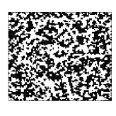
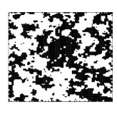
Model 1	Model 2

Figure 4: Realizations from the two higher-order MRF models on a $100\times 100$ lattice, generated by Gibbs sampling. Potential functions for the models are defined in Figure 3.

7.2 Empirical evaluation

In this section we first consider the quality of the approximation of the normalising constant $c$ and the corresponding bounds. Thereafter we evaluate to what extent our $\widetilde{p}(x)$ defined in Section 4 can be used as an approximation to the corresponding $p(x)$.

We first compute the approximate normalising constant $\widetilde{c}$ and the corresponding upper and lower bounds $c_{U}$ and $c_{L}$ for $\nu=1,2,\ldots,18$ for each of our four $\theta$ values. The results are presented in Figure 5.

$\theta=0.4$	$\theta=0.6$	$\theta=0.8$	$\theta=-\ln(\sqrt{2}-1)$

Figure 5: Results for the Ising model: The upper row shows the approximation $\ln(\widetilde{c})$ (solid) and the corresponding upper and lower bounds $\ln(c_{U})$ and $\ln(c_{L})$ (dashed) for $\nu=8,\ldots,18$, and the lower row shows $\ln(c_{U})-\ln(c_{L})$ for $\nu=1$ to $18$.

The upper row shows the approximation $\ln(\widetilde{c})$ together with the bounds $\ln(c_{L})$ and $\ln(c_{U})$ for $\nu=8$ to $19$, whereas the lower row shows $\ln(c_{U})-\ln(c_{L})$ for $\nu=1$ to $19$. For a given value of $\nu$, computation of an approximation takes about the same time for all values of $\theta$, and computation of a bound takes about the same time as evaluating the corresponding approximation. The computation time for one evaluation as a function of $\nu$ is shown in Figure 6(a).

(a) Ising	(b) higher-order MRF

Figure 6: The natural logarithm of the computation times (in seconds) used to compute an approximation or a bound in (a) the Ising model, and (b) the higher-order interaction MRF.

Figure 7 shows similar results for the higher-order MRF models, again for a $100\times 100$ lattice, and corresponding computation times are shown in Figure 6(b).

Model 1	Model 2

Figure 7: Results for the higher-order MRF model: The upper row shows the approximation $\ln(\widetilde{c})$ (solid) and the corresponding upper and lower bounds $\ln(c_{U})$ and $\ln(c_{L})$ (dashed) for $\nu=6,\ldots,18$, and the lower row shows $\ln(c_{U})-\ln(c_{L})$ for $\nu=1$ to $18$.

Not surprisingly, we see that the quality of the approximation and bounds are best for models with weak interactions.

Next we evaluate the quality of the POMM approximation $\widetilde{p}(x)$ given in (28), still on a $100\times 100$ lattice. To do this we consider an independent proposal Metropolis–Hastings algorithm where the MRF $p(x)$ is the target distribution and $\widetilde{p}(x)$ is used as proposal distribution. We use the acceptance rate in such an algorithm to measure the quality of the approximation. It should be emphasised that we do not propose this Metropolis–Hastings as a way to sample from $p(x)$, we just use the acceptance rate of this algorithm to measure the quality of our approximation. It should be noted that in this evaluation test we do not need to compute the normalising constant of the conditional distributions in (28) for all values of the conditioning variables, so we apply the first (and best) POMM approximation variant discussed in the paragraph following (28).

To estimate the quantity we generate $1000$ independent samples from $p(x)$ and corresponding $1000$ independent samples from $\widetilde{p}(x)$, compute the Metropolis–Hastings acceptance probability for each pair and use the average of these numbers as our estimate. For the Ising model we generate perfect samples from $p(x)$ on a $100\times 100$ lattice by first sampling perfectly from the dual random cluster model by coupling from the past (Propp and Wilson, 1996). For the higher-order MRF model we are not able to generate perfect samples, so we instead run a long Gibbs sampling algorithm, and obtain (essentially) independent realizations by sub-sampling this chain. The results for the Ising and higher-order MRF models are given in Figure 8.

(a) Ising		(b) higher-order MRF

Figure 8: Estimated acceptance rates, for $\nu=1,\ldots,18$, for an independent proposal Metropolis–Hastings algorithm with target distribution given by the MRF $p(x)$ on a $100\times 100$ lattice and proposal distribution given by the corresponding POMM approximation $\widetilde{p}(x)$ in (28). (a) Results for the Ising model, from top to bottom the curves are for $\theta=0.4$, $\theta=0.6$, $\theta=0.8$ and $\theta=-\ln(\sqrt{2}-1)$. (b) Results for the higher-order MRFs, the upper and lower curves are for Model 1 and Model 2, respectively, defined in Figures 2 and 3.

For $\theta=0.4$ and $0.6$ in the Ising model we see that we get very good approximations even for quite small values of $\nu$, For $\theta=0.8$ a large values for $\nu$ is needed to get high acceptance rate. For $\theta=-\ln(\sqrt{2}-1)$ the acceptance rate ends at $30\%$ for $\nu=18$, and remembering that this is for a block update of $100\times 100$ variables we think this is quite impressive. For the higher-order MRFs, the acceptance rate for Model 1 becomes very high for the higher values of $\nu$, whereas the results for Model 2 resemble the results for $\theta=-\ln(\sqrt{2}-1)$ in the Ising model.

7.3 Some possible applications

In this section we present some simulation examples that demonstrate some possible applications of the proposed approximations and bounds. All the examples are for MRFs defined on a rectangular lattice, but similar applications for MRFs defined on graphs are of course also possible.

7.3.1 Maximum likelihood estimation

Assume we have observed an image $x$ which we suppose is a realization from an MRF $p(x|\theta)$, where $\theta$ is a scalar parameter. The $p(x|\theta)$ may for example be the Ising model. If we want to estimate $\theta$ the maximum likelihood estimator (MLE) is a natural alternative. As discussed in the introduction the computation of the MLE is complicated by the intractable normalising constant of the MRF. Figure 9

$\nu=2$	$\nu=4$	$\nu=6$
$\nu=8$	$\nu=10$	$\nu=12$
$\nu=14$	$\nu=16$	$\nu=18$

Figure 9: Maximum likelihood example: The identification of an interval in which the MLE for $\theta$ in an Ising model must be located. The estimation is based on a sample from the Ising model with $\theta=0.6$. The plots shows computed upper and lower bounds for the log-likelihood function for different values of $\nu$. The horizontal dotted line is the maximum of the computed lower bounds and the two vertical dotted lines defines the interval in which the maximum likelihood estimate must be located.

illustrates how upper and lower bounds for the normalising constant can be used to identify an interval in which the MLE for $\theta$ must be located. To produce the curves in the figure we first simulated an $x$ from the Ising model with parameter $\theta=0.6$, on an $100\times 100$ rectangular lattice. Assume we want to find the MLE of $\theta$ based on this $x$. We first computed upper and lower bounds for the log-likelihood function by replacing the intractable normalising constant with corresponding upper and lower bounds with $\nu=2$ for $11$ values of $\theta$ on a mesh from $0$ to $2$. The maximum log-likelihood value must clearly be higher than the maximum of the lower bound values. Assuming the log-likelihood function to be concave we can then identify an interval in which the MLE of $\theta$ must lie. Defining a new mesh of $11$ $\theta$ values over this interval we repeated the process for $\nu=4$ and obtain an improved interval, see the upper middle plot in Figure 9. We then repeated this process for $\nu=6,8,\ldots,18$, and the final interval for the MLE shown in the lower right plot in Figure 9 was $(0.6055,0.6123)$. It is important not to confuse this interval with confidence or credibility intervals, the interval computed here is just an interval which, with certainty, includes the MLE of $\theta$. It should be noted that computations of the $2\cdot 11=22$ bounds for the normalising constants can be done in parallel, and for larger values of $\nu$ this is essential for the strategy to be practical. In corresponding simulation experiments with true $\theta$ values equal to $0.4$, $0.8$ and $-\ln(\sqrt{2}-1)$ we obtained the final intervals $(0.4113,0.4115)$, $(0.7716,0.8490)$ and $(0.8234,0.9250)$, respectively. Our bounds are less tight for higher values of $\theta$ and naturally this gives longer intervals for the MLEs when the true $\theta$ value is larger.

7.3.2 Maximum posterior estimation

The approximate Viterbi algorithm discussed in Section 5.2.1 can be used in image analysis applications. Suppose the constructed scene in Figure 10(a), which is in an $89\times 85$ lattice and which we denote by $x$,

Figure 10: Maximum posterior estimation example: True scene used in the maximum posterior estimation and fully Bayesian model examples.

is an unobserved true scene, and assume that a corresponding noisy version $y$ of $x$ is observed. Here we will use a $y$ generated from $x$ by drawing each element of $y$ independently from a normal distribution with unit standard deviation and with means $0$ and $1$ for the white and black areas of $x$, respectively. Assuming the likelihood parameters to be known, and assigning an MRF prior $p(x)$ to $x$, we can estimate $x$ from $y$ by maximising the posterior distribution with respect to $x$, i.e.

$$\widehat{x}=\mbox{arg}\max_{x}\left\{p(x)p(y|x)\right\}.$$ (31)

To compute $\widehat{x}$ is computationally intractable, but by adopting the procedure discussed in Section 5.2.1 we obtain an approximation to $\widehat{x}$. We have done this for the six priors defined above and for values of $\nu$ from $1$ to $18$. The scenes in Figure 11

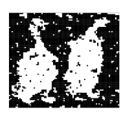
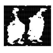
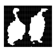
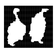
$0.4$	$0.6$	$0.8$	$-\ln(\sqrt{2}-1)$
	Model 1	Model 2

Figure 11: Maximum posterior estimation example: Approximations to $\widehat{x}$ when $\nu=18$ for the four Ising priors (upper row) and the two higher order MRFs (lower row).

show the results for $\nu=18$. It is interesting to observe that the results for the Ising prior with $\beta=0.6$ and $0.8$ are very similar to the results for the higher-order interaction MRFs Models 1 and 2, respectively.

Comparing the results for different values of $\nu$ we find that for the Ising model with $\beta=0.4$ the results are identical for all $\nu=5$ to $18$. For the other seven priors the resulting scenes continued to vary slightly for all the values we used for $\nu$, but in all cases the differences became smaller for higher values of $\nu$. For example, for all these seven priors less than $0.6\%$ of the nodes were assigned different values when $\nu=16$ and $\nu=18$ were used. When comparing the results with the true scene the Ising model with $\beta=0.8$ has the lowest number of misclassifications, with the higher-order MRF Model 2 slightly behind.

7.3.3 Fully Bayesian modelling

Assume again that we have observed a noisy scene $y$ corresponding to a unobserved true image $x$. An alternative to the strategy for estimating $x$ from $y$ discussed above is to adopt a fully Bayesian approach. Here we consider the same simulated $y$ as we did in Section 7.3.2. Then we consider the unobserved $x$ to be a sample from an MRF prior $p(x|\theta)$, where $\theta$ is a parameter vector. For $p(x|\theta)$ we try both the Ising prior (30) and the higher order MRF defined in Section 7.1. The higher order MRF has the ten parameters specified in Figure 3, but to make the model identifiable we fix one parameter corresponding to each of the two maximal cliques. We set the potentials to zero for the configurations where all nodes in a maximal clique are equal. Thus, $\theta$ gets eight elements in this prior. To fully specify the Bayesian model we need to adopt a parametric form for the likelihood $p(y|x,\varphi)$, where $\varphi$ is a parameter vector, and to specify priors for $\theta$ and $\varphi$. For the likelihood we assume the product of normals given in Section 7.3.2 and $\varphi$ contains a mean value and a standard deviation for each of the two possible values of the elements in $x$, i.e. $\varphi=[\mu_{0},\mu_{1},\sigma_{0},\sigma_{1}]$. To avoid problems if all elements of $x$ are assigned to the same value we need to adopt proper priors for the likelihood parameters. For $\mu_{0}$ and $\mu_{1}$ we use independent normal priors with zero mean and standard deviation ten, but to make the model identifiable we add the restriction $\mu_{0}\leq\mu_{1}$. For $\sigma_{0},\sigma_{1}\geq 0$ we a priori assume independent exponential densities with means equal to ten.

To simulate from the resulting posterior $p(x,\theta,\varphi|y)\propto p(\theta)p(\varphi)p(x|\theta)p(y|x,\varphi)$ is computationally infeasible due to the normalising constant of $p(x|\theta)$, but we can simulate from the approximation $\widetilde{p}(x,\theta,\varphi|y)\propto p(\theta)p(\varphi)\widetilde{p}(x|\theta)p(y|x,\varphi)$, where $\widetilde{p}(x|\theta)$ is defined as in (28) and here we adopt the second POMM approximation variant discussed in the paragraph following (28).

. To simulate from $\widetilde{p}(x,\theta,\varphi|y)$ we adopt a Metropolis–Hastings algorithm and alternate between single site updates for the likelihood parameters and the for the components of $x$ and a joint block update for the MRF parameters and $x$. To do Gibbs updates for the likelihood parameters is not feasible, but we use proposals distributions which are close to the full conditionals. More precisely, for each of $\mu_{0}$ and $\mu_{1}$ we find the full conditionals when ignoring the restriction $\mu_{0}<\mu_{1}$ and use these as proposals distributions, and for $\sigma_{0}$ and $\sigma_{1}$ we propose potential new values by proposing values for the corresponding variances from their full conditionals when a very vague inverse gamma prior is assumed. The proposals are then accepted of rejected according to the standard Metropolis–Hastings procedure. In practice essentially all proposals are accepted. In the single site updates for the components of $x$ we generate the potential new state by changing the value of a randomly chosen element in $x$, and in the block update we use a proposal distribution

$$q(\theta^{\prime},x^{\prime}|\theta,\varphi,x)=q(\theta^{\prime}|\theta)\widetilde{p}(x^{\prime}|y,\theta^{\prime},\varphi^{\prime}),$$ (32)

where $q(\theta^{\prime}|\theta)$ is a random walk proposal for $\theta$, and $\widetilde{p}(x^{\prime}|y,\theta^{\prime},\varphi^{\prime})$ is the POMM approximation of the posterior MRF $p(x^{\prime}|y,\theta^{\prime},\varphi^{\prime})\propto\widetilde{p}(x|\theta^{\prime})p(y|x^{\prime},\varphi^{\prime})$. In the random walk proposals for $\theta$ we sample the elements independently from normal distributions centered at the current values and with all standard deviations equal to $0.1$ both for the Ising and higher-order MRF prior cases. We define one MH iteration to consist of one update for each of the likelihood parameters, $89\cdot 85$ single site updates for elements of $x$ and one block update as defined above. Using $\nu=8$ to define the POMM approximations, Figure 12

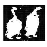
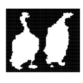
Figure 12: Fully Bayesian model example: Results for a fully Bayesian model, using an Ising prior (upper row) and the higher-order interaction MRF prior (lower row). The leftmost column shows the maximum marginal posterior probability estimate of the underlying scene. The two following columns show estimated posterior distributions for $\mu_{0}$ and $\mu_{1}$, respectively. The rightmost column shows estimated posterior distribution for $\theta$ for the Ising prior and for the eighth parameter in Figure 3 for the higher-order interaction prior.

summarises some simulation results. The left column shows the estimated true scene using the marginal posterior probability estimator for each of the two priors. We observe that the higher-order MRF looks less noisy, and the fraction of wrongly classified values are $4.7\%$ and $4.2\%$ for the Ising and higher-order MRF priors, respectively. The corresponding means of the marginal posterior probabilities for the wrong class labels are $0.102$ and $0.083$, respectively. Thus, the posterior probability for the wrong class is on average $18.5\%$ lower when using the higher-order MRF prior than with the Ising prior. The two middle columns in Figure 12 show the estimated posterior distributions for $\mu_{0}$ and $\mu_{1}$ and we observe that the true values, zero for the second column and one for the third, are far out in the tail of the posterior when using the Ising prior and more centrally located when using the higher-order MRF. All of this demonstrates the potential advantage of using a higher-order MRF prior. The last column in Figure 12 shows the estimated posterior distribution for $\theta$ when using the Ising prior, and the for the eighth parameter in Figure 3 for the higher-order interaction prior. We observe that the variance in the posterior for $\theta$ is quite small, but its value is also well above the phase transition limit. The posterior variability for the parameter in the higher-order interaction prior, however, is very large, and the same is true for the other parameters in this prior. This may indicate that the higher-order interaction prior is over-parameterised and that better results could perhaps have been obtained by adopting a prior with fewer parameters. The best alternative would perhaps be to put a prior also on the interaction order of the model, so that the complexity of the model could adapt automatically to the problem in focus.

7.3.4 Perfect sampling by rejection sampling

The last application of our approximation and bounds we discuss is how it can be used to construct a rejection sampling algorithm generating perfect samples from some MRFs $p(x)$. Let $p(x)=\frac{1}{c}\exp\{U(x)\}$ be a given binary MRF, and let $\widetilde{p}(x)$ denote the corresponding POMM approximation. One can then imagine a rejection sampling algorithm generating candidate samples from $\widetilde{p}(x)$ and accepting a candidate $x$ with probability

$$\alpha(x)=k\cdot\frac{p(x)}{\widetilde{p}(x)}=\widetilde{k}\cdot\frac{\exp\{U(x)\}}{\widetilde{p}(x)},$$ (33)

where $k$ is a constant so that $\alpha(x)\leq 1$ for all $x$, and $\widetilde{k}=k/c$. Clearly the optimal choice for $\widetilde{k}$ is

$$\widetilde{k}_{\mbox{\tiny opt}}=\min_{x}\left\{\widetilde{p}(x)e^{-U(x)}\right\},$$ (34)

but to compute $\widetilde{k}_{\mbox{\tiny opt}}$ is computationally intractable. However, noting that $\ln\left\{\widetilde{p}(x)e^{-U(x)}\right\}$ is a pseudo-Boolean function we can find a lower bound $\ln\widetilde{k}_{\mbox{\tiny bound}}\leq\ln\widetilde{k}_{\mbox{\tiny opt}}$ as discussed in Section 7.3.2, and use $\widetilde{k}=\widetilde{k}_{\mbox{\tiny bound}}$ in (33). It should be noted this procedure implies that we need to compute the normalising constant of the conditional distributions in (28) for all values of the conditioning variables, so when defining the POMM approximation $\widetilde{p}(x)$ we must use the second approximation variant discussed in the paragraph following (28).

The acceptance rate of such a rejection sampling procedure will depend both on the quality of the approximation $\widetilde{p}(x)$ and the ratio $\widetilde{k}_{\mbox{\tiny bound}}/\widetilde{k}_{\mbox{\tiny opt}}$. One should note that the goal in this setting is not to get a very high rejection sampling acceptance rate, but rather to find a good trade off between the acceptance rate and the computation time for generating the proposals, for example by finding the smallest value of $\nu$ that give an acceptance rate above a given threshold. We have tried the procedure on the posterior distributions defined in Section 7.3.2. For the posteriors based on Ising priors with $\beta=0.4$, $0.6$, $0.8$ and $-\ln(\sqrt{2}-1)$ we needed $\nu=5$, $7$, $9$ and $11$, respectively, to obtain acceptance rates above $0.1$, and to get acceptance rates above $0.5$ the corresponding values for $\nu$ are $6$, $8$, $11$ and $13$. Perfect samples from these four posterior distributions can of course alternatively be generated by the coupling from the past procedure of Propp and Wilson (1996). As the rejection sampling procedure requires an initiation step of establishing $\widetilde{p}(x)$ and computing $\widetilde{k}_{\mbox{\tiny bound}}$, coupling from the past is the most efficient alternative whenever only one or a few independent samples are required, but if a large number of samples are wanted the rejection sampling algorithm becomes the best alternative. We have tried the rejection sampling procedure also for the posteriors when adopting the higher order models defined in Section 7.1 as priors, but for this prior we were not able to get useful acceptance rates within reasonable computation times.

7.4 Real data example

In this section we consider a United States cancer mortality map compiled by Riggan et al. (1987). Figure 13 shows

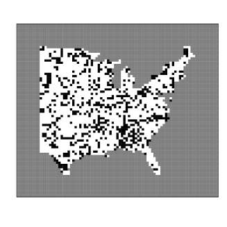
Figure 13: Real data example: U.S. liver and gallbladder cancer mortality map for white males during 1950-1959. Black and white squares denote counties with high and low cancer mortality rates, respectively. The outer box shows the boundary of the extended lattice.

the mortality map for liver and gallbladder cancers for white males in 1950-1959, where black and white squares denote counties with high and low cancer mortality rates, respectively. The data set is previously analysed in Sherman et al. (2006) and Liang (2010), see also the discussion in Liang et al. (2011). In these studies a free boundary autologistic model is compared with a model where the values in the nodes are assumed to be independent, and the conclusions in both studies are that the spatial model gives a much better fit to the data than the independence model.

We define a fully Bayesian model for the data set and a priori assign equal probabilities for three possible models. The two first models are the independence and autologistic models adopted in the previous studies, whereas the third model is an MRF with a $3\times 3$ neighbourhood and higher-order interactions. To reduce the effect of the boundary assumption we include the observed nodes in a larger rectangular lattice as illustrated in Figure 13, and adopt a free boundary assumption for the extended lattice. We let $z$ denote a vector of the observed values and $y$ a vector of the unobserved values, and let $x=(y,z)$ be a vector of all the values in the extended lattice. The dimensions of the rectangular lattice is chosen so that every observed node is at least $10$ nodes away from the border, and the extended lattice is then $78\times 87$. Of the nodes in the extended lattice $34.6\%$ is observed. In the following we first give a more precise specification of the three possible models we allow on the extended lattice and thereafter define prior distributions for the parameters in these models.

The independence model has only one parameter, which we denote by $\theta$, and

$$p_{1}(x|\theta)\propto\exp\left(\theta\sum_{i\in S}x_{i}\right).$$ (35)

In the autologistic model we assume a first-order neighbourhood and assume the horizontal and vertical interactions to be equal. The model then has two parameters, which we denote by $\theta_{0}$ and $\theta_{1}$ and set $\theta=(\theta_{0},\theta_{1})$. Our MRF is then given by

$$p_{2}(x|\theta)\propto\exp\left\{\theta_{0}\sum_{i\sim j}I(x_{i}\neq x_{j})+\theta_{1}\sum_{i\sim j}I(x_{i}=1\cap x_{j}=1)\right\}.$$ (36)

In the $3\times 3$ neighbourhood MRF the maximal cliques are $2\times 2$ blocks of nodes. Also for this model we assume the potential function $V_{\Lambda}(x_{\Lambda})$ to be invariant under rotation of the values in $x_{C}$. The rotational invariance restriction groups the $2^{2\cdot 2}=16$ possible configurations of $x_{C}$ into the six groups illustrated in Figure 14.

$x_{C}$
$V_{\Lambda}(x_{\Lambda};\theta)$	$0$	$\theta^{0}$	$\theta^{1}$	$\theta^{2}$	$\theta^{3}$	$\theta^{4}$

Figure 14: The real data example: The six possible configurations in a $2\times 2$ clique (up to rotation), and the corresponding values of the potential function $V_{\Lambda}(x_{\Lambda};\theta)$ in the $3\times 3$ neighbourhood MRF.

Without loss of generality we can set the potential value for the all zero configuration to zero, and we define one parameter for each of the other five configuration sets, again as shown in Figure 14. The parameter vector in the model is thereby $\theta=(\theta^{0},\ldots,\theta^{4})$ and the MRF is given as

$$p_{3}(x|\theta)\propto\exp\left\{\sum_{\Lambda\in{\cal C}}U_{\Lambda}(x_{\Lambda};\theta)\right\},$$ (37)

where $U_{\Lambda}(x_{\Lambda};\theta)$ is as specified in Figure 14.

As specified above we assume a prior probability $p(m)=1/3$ for each model $m=1,2,3$. Given any of the three models we let the prior for the associated parameters, $p_{m}(\theta)$, be a Gaussian distribution where the components of $\theta$ are independent and Gaussian distributed with zero mean and some variance $\sigma^{2}$. A priori we do not expect very strong interactions for this type of data so we set $\sigma^{2}=1$. The resulting posterior distribution of interest is $p(m,\theta|z)$, but the unobserved vector $y$ makes it hard to simulate from this distribution so in the simulation we focus on $p(m,\theta,y|z)\propto p(m)p_{m}(\theta)p_{m}(y,z|\theta)$. For $m=2$ and $3$ the MRF $p_{m}(y,z|\theta)$ of course contains a computationally intractable normalising constant, so as in Section 7.3.3 we replace $p_{m}(y,z|\theta)$ with a corresponding approximation $\widetilde{p}_{m}(y,z|\theta)$ as defined in (28). As in the fully Bayesian example in Section 7.3.3 we here use the second POMM approximation variant discussed in the paragraph following (28) as this alternative is somewhat faster than the alternative POMM approximation.

The distribution we want to sample is then

$$\widetilde{p}(m,\theta,y|z)\propto p(m)p_{m}(\theta)\widetilde{p}_{m}(y,z|\theta),$$ (38)

and to sample from this distribution we adopt a reversible jump MCMC algorithm (Green, 1995). To get an acceptable trans-dimensional mixing in the MCMC algorithm we found it necessary to include more auxiliary variables. For each of the three models $k=1,2,3$ we added a parameter $\theta_{k}$ and vector $y_{k}$, where $\theta_{1}\in\mathbb{R}$, $\theta_{2}\in\mathbb{R}^{2}$ and $\theta_{3}\in\mathbb{R}^{5}$ and each of the $y_{k}$’s are vectors of the same size as $y$. We assume $(\theta_{k},y_{k})\sim p_{k}(\theta_{k})\widetilde{p}_{k}(y_{k}|\theta_{k},z)$ independently for each $k$ and independent of $(m,\theta,y)$, where $\widetilde{p}_{k}(y_{k}|\theta_{k},z)$ is the POMM approximation of $p_{k}(y_{k}|\theta_{k},z)\propto p_{k}(y_{k},z|\theta_{k})$. To simulate from

$$\widetilde{p}(m,\theta,y,\theta_{1},y_{1},\theta_{2},y_{2},\theta_{3},y_{3}|z)=\widetilde{p}(m,\theta,y|z)\prod_{k=1}^{3}p_{k}(\theta_{k})\widetilde{p}_{k}(y_{k}|\theta_{k},z)$$ (39)

we adopt the reversible jump setup with three types of proposals. The first proposal is a random walk proposal for each of $\theta$, $\theta_{1}$, $\theta_{2}$ and $\theta_{3}$. A separate update is performed for each of these four variables, so a proposed new value for one of them is accepted or rejected before a change for another of the vectors is proposed. The components in the potential new vector are generated independently from Gaussian distributions centered at the current value and with the same variance $\tau^{2}$ for all components. By trial and error we tuned the value of the proposal variance and ended up using $\tau=0.025$. The second proposal type generate potential new values for each of $y$, $y_{1}$, $y_{2}$ and $y_{3}$. Again a proposal followed by an acceptance or rejection is done for each of the vectors separately. For $y_{k},k=1,2,3$ the potential new value is generated from $\widetilde{p}_{k}(y_{k}|\theta_{k},z)$, and the potential new value for $y$ is generated from $\widetilde{p}_{m}(y|\theta_{m},z)$. One can note that the updates for $y_{1}$, $y_{2}$ and $y_{3}$ are Gibbs updates, whereas the update for $y$ is not. The acceptance rate for the $y$ updates is, however, very close to one. The third update type is the only trans-dimensional update. Here new values are proposed for $(m,\theta,y)$ and for one of $(\theta_{1},y_{1})$, $(\theta_{2},y_{2})$ and $(\theta_{3},y_{3})$. First a new value $m^{\prime}$ is proposed for the model indicator $m$. If $m=1$ or $3$ we always set $m^{\prime}=2$, and if $m=2$ we set $m^{\prime}=1$ or $3$ with probabilities a half for each. Thereafter potential new values for $\theta$ and $y$ is deterministically set as $\theta^{\prime}=\theta_{m^{\prime}}$ and $y^{\prime}=y_{m^{\prime}}$. Finally potential new values for $\theta_{m^{\prime}}$ and $y_{m^{\prime}}$ are sampled as $\theta^{\prime}_{m^{\prime}}\sim\mbox{N}(\theta_{m^{\prime}},\tau^{2}I)$ and $y^{\prime}_{m^{\prime}}\sim\widetilde{p}_{m^{\prime}}(y_{m}|\theta^{\prime}_{m^{\prime}},z)$, respectively. Here we use the same variance $\tau^{2}$ as in the random walk proposals discussed above, and $I$ is the identity matrix of the suitable dimension. The proposed new values are then accepted or rejected according to the standard reversible jump MCMC acceptance probability. In particular it is easy to show that the Jacobian determinant occurring in the expression for the acceptance probability equals unity for this kind of proposal.

To check the convergence and mixing properties of the reversible jump MCMC algorithm we ran three independent runs with different starting values. For each of $k=1,2$ and $3$ we had a chain where we initially set $m=k$ and ran 200 iterations without the transdimensional move. The idea here is that the chains should essentially converge conditional on the value of $m$ before we allow the value of $m$ to vary. After these $200$ initial iterations we ran the three chains for an additional $4300$ iterations, now including the transdimensional move. The chain starting with $m=1$ then quickly changed to having $m=2$ and $m=3$ and never returned to the state $m=1$. The chains starting with $m=2$ and $m=3$ never visited the state $m=1$. All three chains had several jumps back and fourth between $m=2$ and $m=3$ as can be seen from Figure 15.

Figure 15: Real data example: For the Markov chain simulation starting at $m=1$, trace plot of the simulated values for $m$.

In the analysis of the Markov chain runs we discard the first $500$ iterations of each run as burn-in, and use all three runs to estimate the quantities of interest. We estimate the posterior probability for model $m=3$ by the fraction of times the chains are visiting this state, and get $\widehat{p}(m=3|z)=0.680$. To evaluate the uncertainty in this number we split the chains into intervals of $100$ iterations and estimate $p(m=3|z)$ based on each of these intervals. These estimates are close to being uncorrelated so, considering them as independent, we use them to construct an approximate $95\%$ credibility $t$-interval for $p(m=3|z)$. The interval becomes $[0.619,0.741]$, clearly showing that $m=3$ is the model with highest a posteriori probability. This demonstrates that even for data sets where the interactions are quite weak there can be a need for including higher-order interactions. Figures 16 and

$\theta_{0}$	$\theta_{1}$

Figure 16: Real data example: Histograms of the simulated posterior values for $\theta_{0}$ and $\theta_{1}$ when $m=2$.

17 show estimates of the marginal distributions for the model

$\theta_{0}$	$\theta_{1}$	$\theta_{2}$
$\theta_{3}$	$\theta_{4}$

Figure 17: Real data example: Histograms of the simulated posterior values for $\theta_{0},\ldots,\theta_{4}$ when $m=3$.

parameters for model $m=2$ and $m=3$, respectively. One should note that the spread of all of these parameters are well within the variability of the corresponding standard normal prior, so our prior here should not be very influential on these results. We also observe that all parameters, both for model $m=2$ and $3$, are significantly smaller than zero. This reflects that zero is the dominating value of the data set and that we in both models have chosen to set the potential for maximal cliques with only zero values to the reference value of zero.

8 Closing remarks

In this report we have shown how we can derive an approximate forward-backward algorithm by studying how to approximate the pseudo-Boolean energy function during the summation process. This approximation can then be used to work with statistical models such as MRFs. It allows us to produce approximations and bounds of the normalising constant and likelihood for models that would normally be too computationally heavy to work with directly. It also gives POMM approximations of MRFs that can be used as a surrogate for MRFs in more complicated model setups. We have demonstrated the accuracy of the approximation and bounds through simple experiments with the Ising model and a higher-order interaction model, and demonstrated some potential applications by simulation experiments. We have also applied our approximation to a real life data set and here demonstrated that higher-order interactions may be important even for data sets with weak interactions. We round off now with some possible future extensions as well as some closing remarks.

The approximation we have defined was inspired by the work in Tjelmeland and Austad (2012) and there are many parallels between the two. There the energy function was represented as a binary polynomial and small interactions was dropped while running the forward-backward algorithm. This worked reasonably well, but one may worry that dropping many smalls interactions may produce an approximation no better than when dropping one large interaction. Moreover, for models with strong interactions the approximation in Tjelmeland and Austad (2012) would either include too many terms and thus explode in run-time, or if the cutoff level was set low enough to run the algorithm, exclude so many of the interactions that the approximation became uninteresting. In a sense the work in this report has been an effort to deal with these issues. We have a clearly defined approximation criterion and the construction of the algorithm allows for much more direct control over the run time. Also, by not just dropping small terms, but approximating the pseudo-Boolean function in such a way that we minimise the error sum of squares we manage to get better approximations of the models with stronger interactions.

In our setting the sample space of the pseudo-Boolean function has a probability measure on it, however in our discussion of approximating pseudo-Boolean functions we have considered each state in the sample space as equally important. Assuming we are interested in approximating the normalising constant, this is probably far from optimal and is reflected in our results. As we can see for the Ising model our approximation works better the smaller the interaction parameter $\theta$. Our initial approximation attempts to spread the error of removing interactions as evenly as possible among the states. Ideally, we would like to have small errors in states with a corresponding high probability, and larger errors in states with low probability. To get this approximation we should replace the SSE in (4) with a weighted error sum of squares. This problem has also been studied in the literature, see for instance Ding et al. (2008, 2010). However, unlike the unweighted case an explicit solution is not readily available for a probability density like the MRF. The iterative method of removing interactions does not work here, nor can we group the equations like we do with the SOIR approximation.

In all our examples we consider MRFs defined on a lattice and assume the potential functions to be translational invariant. Our approximations and bounds are, however, also valid for MRFs defined on an arbitrary graph and applications of the approximation and bounds in such situations is something we want to explore in the future.

Appendix A Proof of Theorem 3

Expanding $\mbox{SSE}(f,\tilde{\tilde{f}})=\sum_{x\in\Omega}\left\{f(x)-\tilde{\tilde{f}}(x)\right\}^{2}$ we get,

$$\sum_{x\in\Omega}\left\{f(x)-\tilde{\tilde{f}}(x)\right\}^{2}=\sum_{x\in\Omega}\left\{f(x)-\tilde{f}(x)+\tilde{f}(x)-\tilde{\tilde{f}}(x)\right\}^{2}$$

$$=\sum_{x\in\Omega}\left\{f(x)-\tilde{f}(x)\right\}^{2}+\sum_{x\in\Omega}\left\{\tilde{f}(x)-\tilde{\tilde{f}}(x)\right\}^{2}+\sum_{x\in\Omega}\{f(x)-\tilde{f}(x)\}\{\tilde{f}(x)-\tilde{\tilde{f}}(x)\}$$

$$=\mbox{SSE}(f,\tilde{f})+\mbox{SSE}(\tilde{f},\tilde{\tilde{f}})+\sum_{x\in\Omega}\{f(x)-\tilde{f}(x)\}\tilde{f}(x)-\sum_{x\in\Omega}\{f(x)-\tilde{f}(x)\}\tilde{\tilde{f}}(x).$$

To prove the theorem it is thereby sufficient to show that,

$$\sum_{x\in\Omega}\{f(x)-\tilde{f}(x)\}\tilde{f}(x)-\sum_{x\in\Omega}\{f(x)-\tilde{f}(x)\}\tilde{\tilde{f}}(x)=0.$$

First recall that we from (5) know that,

$$\sum_{x\in\Omega_{\lambda}}\left\{f(x)-\tilde{f}(x)\right\}=0,\text{ }\forall\text{ }\lambda\in\tilde{S}.$$ (40)

Also, since $\tilde{\tilde{S}}\subseteq\tilde{S}$,

$$\sum_{x\in\Omega_{\lambda}}\left\{f(x)-\tilde{f}(x)\right\}=0,\text{ }\forall\text{ }\lambda\in\tilde{\tilde{S}}.$$ (41)

We study the first term, $\sum_{x\in\Omega}\{f(x)-\tilde{f}(x)\}\tilde{f}(x)$, expand the expression for $\tilde{f}(x)$ outside the parenthesis and change the order of summation,

$$\sum_{x\in\Omega}\{f(x)-\tilde{f}(x)\}\tilde{f}(x) =\sum_{x\in\Omega}\left[\{f(x)-\tilde{f}(x)\}\sum_{\Lambda\in\tilde{S}}\tilde{\beta}^{\Lambda}\prod_{k\in\Lambda}x_{k}\right]$$

$$=\sum_{\Lambda\in\tilde{S}}\left(\tilde{\beta}^{\Lambda}\sum_{x\in\Omega}\left[\prod_{k\in\Lambda}x_{k}\{f(x)-\tilde{f}(x)\}\right]\right)$$

$$=\sum_{\Lambda\in\tilde{S}}\left[\tilde{\beta}^{\Lambda}\sum_{x\in\Omega_{\Lambda}}\left\{f(x)-\tilde{f}(x)\right\}\right]=0,$$

where the last transition follows from (40). Using (41) we can correspondingly show that $\sum_{x\in\Omega}\{f(x)-\tilde{f}(x)\}\tilde{\tilde{f}}(x)=0$.

Appendix B Proof of Theorem 4

We study the error sum of squares,

$$\sum_{x\in\Omega}\left\{f(x)-\tilde{f}(x)\right\}^{2} =\sum_{x\in\Omega}\left[\{f(x)-\tilde{f}(x)\}f(x)\right]-\sum_{x\in\Omega}\left[\{f(x)-\tilde{f}(x)\}\tilde{f}(x)\right]$$

$$=\sum_{x\in\Omega}\left[\sum_{\Lambda\in S}\beta^{\Lambda}\{f(x)-\tilde{f}(x)\}\prod_{k\in\Lambda}x_{k}\right]-\sum_{x\in\Omega}\left[\sum_{\Lambda\in\tilde{S}}\tilde{\beta}^{\Lambda}\{f(x)-\tilde{f}(x)\}\prod_{k\in\Lambda}x_{k}\right]$$

$$=\sum_{\Lambda\in S}\beta^{\Lambda}\left[\sum_{x\in\Omega_{\Lambda}}\{f(x)-\tilde{f}(x)\}\right]-\sum_{\Lambda\in\tilde{S}}\tilde{\beta}^{\Lambda}\left[\sum_{x\in\Omega_{\Lambda}}\{f(x)-\tilde{f}(x)\}\right],$$

where the second sum is always zero by (41). Since $\tilde{S}\subseteq S$, the first sum can be further split into two parts,

$$\sum_{\Lambda\in S}\beta^{\Lambda}\left[\sum_{x\in\Omega_{\Lambda}}\{f(x)-\tilde{f}(x)\}\right]=\sum_{\Lambda\in\tilde{S}}\beta^{\Lambda}\left[\sum_{x\in\Omega_{\Lambda}}\{f(x)-\tilde{f}(x)\}\right]+\sum_{\Lambda\in S\setminus\tilde{S}}\beta^{\Lambda}\left[\sum_{x\in\Omega_{\Lambda}}\{f(x)-\tilde{f}(x)\}\right],$$

where once again the first sum is zero.

Appendix C Proof of Theorem 5

From Theorem 1 it follows that it is sufficient to consider a function $f(x)$ with non-zero interactions $\beta^{\Lambda}$ only for $\Lambda\in S_{\{i,j\}}$, since we only need to focus on the interactions we want to remove. Thus we have

$$f(x)=\sum_{\Lambda\in S_{\{i,j\}}}\beta^{\Lambda}\prod_{k\in\Lambda}x_{k}\mbox{\leavevmode\nobreak\ \leavevmode\nobreak\ \leavevmode\nobreak\ and\leavevmode\nobreak\ \leavevmode\nobreak\ \leavevmode\nobreak\ }\widetilde{f}(x)=\sum_{\Lambda\in\widetilde{S}}\widetilde{\beta}^{\Lambda}\prod_{k\in\Lambda}x_{k},$$

and we need to show that then

$$\tilde{\beta}^{\Lambda}=\left\{\begin{array}[]{@{}ll}-\frac{1}{4}\beta^{\Lambda\cup\{i,j\}}&\mbox{\leavevmode\nobreak\ \leavevmode\nobreak\ if $\Lambda\cup\{i,j\}\in S$},\\ \hskip 7.39755pt\frac{1}{2}\beta^{\Lambda\cup\{i\}}&\mbox{\leavevmode\nobreak\ \leavevmode\nobreak\ if $\Lambda\cup\{i\}\in S$ and $\Lambda\cup\{j\}\not\in S$},\\ \hskip 7.39755pt\frac{1}{2}\beta^{\Lambda\cup\{j\}}&\mbox{\leavevmode\nobreak\ \leavevmode\nobreak\ if $\Lambda\cup\{i\}\not\in S$ and $\Lambda\cup\{j\}\in S$},\\ \hskip 7.39755pt0&\mbox{\leavevmode\nobreak\ \leavevmode\nobreak\ otherwise.}\end{array}\right.$$ (42)

We start by defining the sets

$$R_{\Lambda}=\{\Lambda\setminus\{i\},\Lambda\setminus\{j\},\Lambda\setminus\{i,j\}\}\mbox{\leavevmode\nobreak\ \leavevmode\nobreak\ for $\Lambda\in S_{\{i,j\}}$},$$

and note that these sets are disjoint, and, since we have assumed $S$ to be dense, $R_{\Lambda}\subseteq\widetilde{S}$. Defining also the residue set

$$T=\widetilde{S}\setminus\left(\bigcup_{\Lambda\in S_{\{i,j\}}}R_{\Lambda}\right)$$

we may write the approximation error $f(x)-\widetilde{f}(x)$ in the following form,

$$f(x)-\widetilde{f}(x)=\sum_{\Lambda\in S_{\{i,j\}}}\left\{\left(\beta^{\Lambda}x_{i}x_{j}-\sum_{\lambda\in R_{\Lambda}}\widetilde{\beta}^{\lambda}\prod_{k\in\Lambda\setminus\lambda}x_{k}\right)\prod_{k\in\Lambda\setminus\{i,j\}}x_{k}\right\}-\sum_{\Lambda\in T}\widetilde{\beta}^{\Lambda}\prod_{k\in\Lambda}x_{k}.$$

Defining

$$\Delta f^{\Lambda}(x_{i},x_{j})=\beta^{\Lambda}x_{i}x_{j}-\sum_{\lambda\in R_{\Lambda}}\widetilde{\beta}^{\lambda}\prod_{k\in\Lambda\setminus\lambda}x_{k}=\beta^{\Lambda}x_{i}x_{j}-\left(\widetilde{\beta}^{\Lambda\setminus\{i,j\}}+\widetilde{\beta}^{\Lambda\setminus\{j\}}x_{i}+\widetilde{\beta}^{\Lambda\setminus\{i\}}x_{j}\right)$$

we have

$$f(x)-\widetilde{f}(x)=\sum_{\Lambda\in S_{\{i,j\}}}\Delta f^{\Lambda}(x_{i},x_{j})\prod_{k\in\Lambda\setminus\{i,j\}}x_{k}-\sum_{\Lambda\in T}\widetilde{\beta}^{\Lambda}\prod_{k\in\Lambda}x_{k}.$$ (43)

Inserting this into (5) and switching the order of summation we get

$$\sum_{x\in\Omega_{\lambda}}\left\{f(x)-\widetilde{f}(x)\right\}=\sum_{x\in\Omega_{\lambda}}\left(\sum_{\Lambda\in S_{\{i,j\}}}\Delta f^{\Lambda}(x_{i},x_{j})\prod_{k\in\Lambda\setminus\{i,j\}}x_{k}-\sum_{\Lambda\in T}\widetilde{\beta}^{\Lambda}\prod_{k\in\Lambda}x_{k}\right)$$

$$=\sum_{\Lambda\in S_{\{i,j\}}}\left(\sum_{x\in\Omega_{\lambda}}\Delta f^{\Lambda}(x_{i},x_{j})\prod_{k\in\Lambda\setminus\{i,j\}}x_{k}\right)-\sum_{\Lambda\in T}\left(\sum_{x\in\Omega_{\lambda}}\widetilde{\beta}^{\Lambda}\prod_{k\in\Lambda}x_{k}\right)$$

$$=\sum_{\Lambda\in S_{\{i,j\}}}\left(\sum_{x\in\Omega_{\lambda\cup(\Lambda\setminus\{i,j\}}}\Delta f^{\Lambda}(x_{i},x_{j})\right)-\sum_{\Lambda\in T}\left(\sum_{x\in\Omega_{\lambda\cup T}}\widetilde{\beta}^{\Lambda}\right)=0\mbox{\leavevmode\nobreak\ \leavevmode\nobreak\ \leavevmode\nobreak\ for all $\lambda\in\widetilde{S}$}$$ (44)

We now proceed to show that this system of equations has a solution where $\widetilde{\beta}^{\Lambda}=0$ for $\Lambda\in T$ and $\sum_{x\in\Omega_{\lambda\cup(\Lambda\setminus\{i,j\}}}\Delta f^{\Lambda}(x_{i},x_{j})=0$ for each $\Lambda\in S_{\{i,j\}}$. Obviously for each $\Lambda$ the function $\Delta f^{\Lambda}(x_{i},x_{j})$ has only our possible values, namely $\Delta f^{\Lambda}(0,0)$, $\Delta f^{\Lambda}(1,0)$, $\Delta^{\Lambda}(0,1)$ and $\Delta f^{\Lambda}(1,1)$. Thus the sum $\sum_{x\in\Omega_{\lambda\cup(\Lambda\setminus\{i,j\}}}\Delta f^{\Lambda}(x_{i},x_{j})$ is simply given as a sum over these four values multiplied by the number of times they occur. Consider first the case where $\lambda$, and thereby also $\lambda\cup(\Lambda\setminus\{i,j\})$ does not contain $i$ or $j$. Then the four values $\Delta f^{\Lambda}(0,0)$, $\Delta f^{\Lambda}(1,0)$, $\Delta^{\Lambda}(0,1)$ and $\Delta f^{\Lambda}(1,1)$ will occur the same number of times, so

$$\sum_{x\in\Omega_{\lambda\cup(\Lambda\setminus\{i,j\})}}\Delta f^{\Lambda}(x_{i},x_{j})=\frac{|\Omega_{\lambda\cup(\Lambda\setminus\{i,j\}}|}{4}\left(\Delta f^{\Lambda}(0,0)+\Delta f^{\Lambda}(1,0)+\Delta f^{\Lambda}(0,1)+\Delta f^{\Lambda}(1,1)\right).$$

Next consider the case when $\lambda$, and thereby also $\lambda\cup(\Lambda\setminus\{i,j\})$, contains $i$, but not $j$. Then $x_{i}=1$ in all terms in the sum, so the values $\Delta f^{\Lambda}(0,0)$ and $\Delta f^{\Lambda}(0,1)$ will not occur, whereas the values $\Delta f^{\Lambda}(1,0)$ and $\Delta f^{\Lambda}(1,1)$ will occur the same number of times. Thus,

$$\sum_{x\in\Omega_{\lambda\cup(\Lambda\setminus\{i,j\})}}\Delta f^{\Lambda}(x_{i},x_{j})=\frac{|\Omega_{\lambda\cup(\Lambda\setminus\{i,j\}}|}{2}\left\{\Delta f^{\Lambda}(1,0)+\Delta f^{\Lambda}(1,1)\right\}.$$

When $\lambda$ contains $j$, but not $i$ we correspondingly get

$$\sum_{x\in\Omega_{\lambda\cup(\Lambda\setminus\{i,j\})}}\Delta f^{\Lambda}(x_{i},x_{j})=\frac{|\Omega_{\lambda\cup(\Lambda\setminus\{i,j\}}|}{2}\left\{\Delta f^{\Lambda}(0,1)+\Delta f^{\Lambda}(1,1)\right\}.$$

The final case, that $\lambda$ contains both $i$ and $j$, will never occur since $\lambda\in\widetilde{S}$ and all interaction involving both $i$ and $j$ have been removed from $\widetilde{S}$. We can now reach the conclusion that if we can find a solution for

$$\Delta f^{\Lambda}(0,0)+\Delta f^{\Lambda}(1,0)+\Delta f^{\Lambda}(0,1)+\Delta(1,1) =0,$$

$$\Delta f^{\Lambda}(1,0)+\Delta f^{\Lambda}(1,1) =0,$$

$$\Delta f^{\Lambda}(0,1)+\Delta f^{\Lambda}(1,1) =0,$$

for all $\Lambda\in S_{\{i,j\}}$ we also have a solution for (44) as discussed above. Using our expression for $\Delta f^{\Lambda}(x_{i},x_{j})$, the above three equations become

$$\beta^{\Lambda}-\left(4\widetilde{\beta}^{\Lambda\setminus\{i,j\}}+2\widetilde{\beta}^{\Lambda\setminus\{i\}}+2\widetilde{\beta}^{\Lambda\setminus\{j\}}\right) =0,$$

$$\beta^{\Lambda}-\left(2\widetilde{\beta}^{\Lambda\setminus\{i,j\}}+\widetilde{\beta}^{\Lambda\setminus\{i\}}+2\widetilde{\beta}^{\Lambda\setminus\{j\}}\right) =0,$$

$$\beta^{\Lambda}-\left(2\widetilde{\beta}^{\Lambda\setminus\{i,j\}}+2\widetilde{\beta}^{\Lambda\setminus\{i\}}+\widetilde{\beta}^{\Lambda\setminus\{j\}}\right) =0.$$

Since the sets $R_{\Lambda}$ are disjoint, the three equations above can be solved separately for each $\Lambda$, and the solution is $\widetilde{\beta}^{\Lambda\setminus\{i,j\}}=-\frac{1}{4}\beta^{\Lambda}$ and $\widetilde{\beta}^{\Lambda\setminus\{i\}}=\widetilde{\beta}^{\Lambda\setminus\{j\}}=\frac{1}{2}\beta^{\Lambda}$. Together with $\widetilde{\beta}^{\Lambda}=0$ for $\Lambda\in T$ this is equivalent to (10) in the theorem. Inserting the values we have found for $\widetilde{\beta}^{\Lambda}$ in (43) we get

$$\Delta f^{\Lambda}(x_{i},x_{j})=\left(x_{i}x_{j}+\frac{1}{4}-\frac{1}{2}x_{i}-\frac{1}{2}x_{j}\right)\beta^{\Lambda}.$$

Inserting this into the above expression for $f(x)-\widetilde{f}(x)$, and using that we know $\widetilde{\beta}^{\Lambda}=0$ for $\Lambda\in T$ we get (11) given in the theorem.

References

- (1)
- Austad (2011) Austad, H. M. (2011). Approximations of Binary Markov random fields, PhD thesis, Norwegian University of Science and Technology. Thesis number 292:2011. Available from http://urn.kb.se/resolve?urn=urn:nbn:no:ntnu:diva-14922.
- Besag (1974) Besag, J. (1974). Spatial interaction and the statistical analysis of lattice systems, Journal of the Royal Statistical Society, Series B 36: 192–225.
- Besag (1986) Besag, J. (1986). On the statistical analysis of dirty pictures (with discussion), Journal of the Royal Statistical Society, Series B 48: 259–302.
- Clifford (1990) Clifford, P. (1990). Markov random fields in statistics, in G. R. Grimmett and D. J. A. Welsh (eds), Disorder in Physical Systems, Oxford University Press, pp. 19–31.
- Cowell et al. (2007) Cowell, R. G., Dawid, A. P., Lauritzen, S. L. and Spiegelhalter, D. J. (2007). Probabilistic Networks and Expert Systems, Exact Computational Methods for Bayesian Networks, Springer, London.
- Cressie (1993) Cressie, N. A. C. (1993). Statistics for Spatial Data, 2 edn, John Wiley, New York.
- Cressie and Davidson (1998) Cressie, N. and Davidson, J. (1998). Image analysis with partially ordered Markov models, Computational Statistics and Data Analysis 29: 1–26.
- Ding et al. (2008) Ding, G., Lax, R., Chen, J. and Chen, P. P. (2008). Formulas for approximating pseudo-Boolean random variables, Discrete Applied Mathematics 156: 1581–1597.
- Ding et al. (2010) Ding, G., Lax, R., Chen, J., Chen, P. P. and Marx, B. D. (2010). Transforms of pseudo-Boolean random variables, Discrete Applied Mathematics 158: 13–24.
- Friel et al. (2009) Friel, N., Pettitt, A. N., Reeves, R. and Wit, E. (2009). Bayesian inference in hidden Markov random fields for binary data defined on large lattices, Journal of Computational and Graphical Statistics 18: 243–261.
- Friel and Rue (2007) Friel, N. and Rue, H. (2007). Recursive computing and simulation-free inference for general factorizable models, Biometrika 94: 661–672.
- Gelman and Meng (1998) Gelman, A. and Meng, X.-L. (1998). Simulating normalizing constants: from importance sampling to bridge sampling to path sampling, Statistical Science 13: 163–185.
- Geyer and Thompson (1995) Geyer, C. J. and Thompson, E. A. (1995). Annealing Markov chain Monte Carlo with applications to ancestral inference, Journal of American Statistical Association 90: 909–920.
- Grabisch et al. (2000) Grabisch, M., Marichal, J. L. and Roubens, M. (2000). Equivalent representations of set functions, Mathematics of Operations Research 25: 157–178.
- Green (1995) Green, P. J. (1995). Reversible jump MCMC computation and Bayesian model determination, Biometrika 82: 711–732.
- Gu and Zhu (2001) Gu, M. G. and Zhu, H. T. (2001). Maximum likelihood estimation for spatial models by Markov chain Monte Carlo stochastic approximation, Journal of the Royal Statistical Society, Series B 63: 339–355.
- Hammer and Holzman (1992) Hammer, P. L. and Holzman, R. (1992). Approximations of pseudo-Boolean functions; applications to game theory, Methods and Models of Operation Research 36: 3–21.
- Hammer and Rudeanu (1968) Hammer, P. L. and Rudeanu, S. (1968). Boolean Methods in Operation Research and Related Areas, Springer, Berlin.
- Künsch (2001) Künsch, H. R. (2001). State space and hidden Markov models, in O. E. Barndorff-Nielsen, D. R. Cox and C. Klüppelberg (eds), Complex Stochastic Systems, Chapman & Hall/CRC.
- Liang (2010) Liang, F. (2010). A double Metropolis–Hastings sampler for spatial models with intractable normalizing constants, Journal of Statistical Computation and Simulation 80: 1007–1022.
- Liang et al. (2011) Liang, F., Liu, C. and Carroll, R. (2011). Advanced Markov Chain Monte Carlo Methods: Learning from Past Samples, Wiley.
- Møller et al. (2006) Møller, J., Pettitt, A., Reeves, R. and Berthelsen, K. (2006). An efficient Markov chain Monte Carlo method for distributions with intractable normalising constants, Biometrika 93: 451–458.
- Propp and Wilson (1996) Propp, J. G. and Wilson, D. B. (1996). Exact sampling with coupled Markov chains and applications to statistical mechanics, Random Stuctures and Algorithms 9: 223–252.
- Reeves and Pettitt (2004) Reeves, R. and Pettitt, A. N. (2004). Efficient recursions for general factorisable models, Biometrika 91: 751–757.
- Riggan et al. (1987) Riggan, W. B., Creason, J. P., Nelson, W. C., Manton, K. G., Woodbury, M. A., Stallard, E., Pellom, A. C. and Beaubier, J. (1987). U.S. Cancer Mortality Rates and Trends, 1950-1979, Vol. IV (U.S. Goverment Printing Office, Washington, DC: Maps, U.S. Environmental Protection Agency).
- Sherman et al. (2006) Sherman, M., Apanasovich, T. V. and Carroll, R. J. (2006). On estimation in binary autologistic spatial models, Journal of Statistical Computation and Simulation 76: 167–179.
- Tjelmeland and Austad (2012) Tjelmeland, H. and Austad, H. (2012). Exact and approximate recursive calculations for binary Markov random fields defined on graphs, Journal of Computational and Graphical Statistics 21: 758–780.
- Viterbi (1967) Viterbi, A. J. (1967). Error bounds for convolutional codes and an asymptotic optimum decoding algorithm, IEEE Transactions on Information Theory 13: 260–269.