Liquidity costs: a new numerical methodology and an empirical study

Abstract

We consider rate swaps which pay a fixed rate against a floating rate in presence of bid-ask spread costs. Even for simple models of bid-ask spread costs, there is no explicit strategy optimizing an expected function of the hedging error. We here propose an efficient algorithm based on the stochastic gradient method to compute an approximate optimal strategy without solving a stochastic control problem. We validate our algorithm by numerical experiments. We also develop several variants of the algorithm and discuss their performances in terms of the numerical parameters and the liquidity cost.

Keywords: Interest rates derivatives, Optimization, Stochastic Algorithms.

1 Introduction

Classical models in financial mathematics usually assume that markets are perfectly liquid. In particular, each trader can buy or sell the amount of assets he/she needs at the same price (the “market price”), and the trader’s decisions do not affect the price of the asset. In practice, the assumption of perfect liquidity is never satisfied but the error due to illiquidity is generally negligible with respect to other sources of error such as model error or calibration error, etc.

However, the perfect liquidity assumption does not hold true in practice for interest rate derivatives market: the liquidity costs to hedge interest rate derivatives are highly time varying. Even though there exist maturities for which zero-coupon bonds are liquid, bonds at intermediate maturities may be extremely illiquid (notice that the underlying interest rate is not directly exchangeable). Therefore, hedging such derivatives absolutely needs to take liquidity risk into account. In this context, defining and computing efficient approximate perfect hedging strategies is a complex problem. The main purpose of this paper is to show that stochastic optimization methods are powerful tools to treat it without solving a necessarily high dimensional stochastic control problem, under the constraints that practitioners need to trade at prescribed dates and that relevant strategies depend on a finite number of parameters. More precisely, we construct and analyze an efficient original numerical method which provides practical strategies facing liquidity costs and minimizing hedging errors.

The outline of the paper is as follows. Section 2 introduces the model. In Section 3, we present our numerical method and analyze it from a theoretical point of view within the framework of a Gaussian yield curve model. Section 4 is devoted to a numerical validation in the idealistic perfect liquidity context. In Section 5, we develop an empirical study of the efficiency of our algorithm in the presence of liquidity costs.

2 Our settings: swaps with liquidity cost

2.1 A short reminder on swaps and swaptions hedging without liquidity cost

One of the most common swaps on the interests rate market is as follows. The counterparts exchange two coupons: the first one is generated by a bond (with a constant fixed interest rate) and the second one is generated by a floating rate (e.g. a LIBOR).

Definition 1.

In a perfectly liquid market, the price at time $t$ of a zero-coupon bond paying $1$ at time $T$ is denoted by $B(t,T)$. The linear forward rate $L(T_{F},T_{B},T_{E})$ is the fair rate decided at time $T_{F}$ determining the amount at time $T_{E}$ obtained by investing 1 at time $T_{B}$. The following relation is satisfied:

$$L\left(T_{F},T_{B},T_{E}\right)=\dfrac{1}{T_{E}-T_{B}}\left(\dfrac{B\left(T_{F},T_{B}\right)}{B\left(T_{F},T_{E}\right)}-1\right).$$ (1)

A swap contract specifies:

• an agreement date $t$

• a time line $(t\leq)~{}T_{0}<\cdots<T_{N}$

• a fixed interest rate $r$

• a floating interest rate

• the payoff at each time $T_{i}$ ($1\leq i\leq N$), that is,

  $$P(i):=\left(T_{i}-T_{i-1}\right)\left(r-L\left(T_{i-1},T_{i-1},T_{i}\right)\right).$$ (2)

  From (1), we deduce the equivalent expression

  $$P(i)=r\left(T_{i}-T_{i-1}\right)-\dfrac{1}{B(T_{i-1},T_{i})}+1.$$ (3)

In the sequel, we consider that the fixed rate $r$ is chosen at the money (thus the swap at time $t$ has zero value), and that the swap fixed coupons are received by the trader.

In the idealistic framework of a market without liquidity cost, the trader buys or sells quantities of zero-coupon bonds at the same price (i.e. the market price), and there exists a discrete time perfect hedging strategy which is independent of any model of interest rates. In view of (3), the replication of the payoff $P(i)$ at time $T_{i}$ can be split into three parts:

• the fixed part $r(T_{i}-T_{i-1})$ is replicated statically at time $t$ by selling $r(T_{i}-T_{i-1})$ zero-coupon bonds with maturity $T_{i}$.

• the floating part $1/B(T_{i-1},T_{i})$ is replicated dynamically at time $T_{i-1}$ by buying $1/B(T_{i-1},T_{i})$ zero-coupon bonds with maturity $T_{i}$. The price of this transaction is equal to $1$.

• the last (fixed) part $1$ is used at time $T_{i}$ to buy $1/B(T_{i},T_{i+1})$ zero-coupon bonds with maturity $T_{i+1}$.

It is easy to see that this strategy is self-financing at times $T_{1},\cdots,T_{N-1}$. To make it self-financing at time $t$ also, at this date one buys $1$ zero-coupon bond with maturity $T_{0}$ and sells $1$ zero-coupon bond with maturity $T_{N}$.

To summarize, in the idealistic framework, we do not need to consider $(\mathcal{F}_{\theta},\theta\geq 0)$ adapted hedging strategies, where $(\mathcal{F}_{\theta},\theta\geq 0)$ is the filtration generated by the observations (short rates, derivative prices, etc.) in continuous time, and we may restrict the admissible strategies to be adapted to the filtration generated by the observations at times $\{t,T_{0},T_{1},\cdots,T_{N}\}$.

2.2 Hypotheses on markets with liquidity costs

We now consider markets with liquidity costs and need to precise our liquidity cost model. In all the sequel $T_{-1}$ denotes $t$.

Hypothesis 2.

We assume that, for all $-1\leq j<i\leq N$, the number $\pi(j,i)$ of zero-coupon bonds with maturity $T_{i}$ bought or sold at time $T_{j}$ is measurable with respect to the filtration generated by $(R_{t},R_{T_{0}},\cdots,R_{T_{j}})$. That means that the admissible strategies do not depend on the evolution of the rate $R_{\theta}$ between two tenor dates $T_{m}$ and $T_{m+1}$.

Denote by $\Psi(T,U,\pi)$ the buy or sell price for $\pi$ zero coupon bonds. In perfectly liquid markets, $\Psi(T,U,\pi)$ is the linear function $B(T,U)\pi$, where $B(T,U)$ is defined in Definition 1. In the presence of liquidity costs, $\Psi(T,U,\pi)$ becomes a non-linear function of $\pi$.

Hypothesis 3.

For all $T$ and $U$, the price $\Psi(T,U,\pi)$ is a $C^{1}(\mathbb{R})$, increasing, convex one-to-one map of $\pi$ from $\mathbb{R}$ to $\mathbb{R}$, and $\Psi(T,U,0)=0$.

Under the preceding hypothesis, the function $\Psi$ is positive when $\pi>0$ and negative when $\pi<0$.

In the context of the swap we set

$$\Psi_{i,j}(\pi):=\Psi(T_{i},T_{j},\pi)$$ (4)

and we only consider self-financing strategies, that is, satisfying

$$\forall\,0\leq j\leq N-1,\quad\sum_{-1\leq k<j}\pi(k,j)+P(j)=\sum_{j<i\leq N}\Psi_{j,i}(\pi(j,i)).$$ (5)

2.3 Optimization objective

In the presence of liquidity risk, the market is not complete any more and the practitioners need to build a strategy which minimizes a given function $S$ (e.g. a risk measure) of the hedging error. Such strategies are usually obtained by solving stochastic control problems. These problems require high complexity numerical algorithms which are too slow to be used in practice. We here propose an efficient and original numerical method to compute approximate optimal strategies. As the perfect hedging leads to a null portfolio at time $T_{N}$, we have to solve the optimization problem

$$\inf_{\boldsymbol{\pi}\in\Pi}\mathbb{E}\left[S(W^{\boldsymbol{\pi}})\right],$$ (6)

where $W^{\boldsymbol{\pi}}$ is the terminal wealth (at time $T_{N}$) given the strategy $\boldsymbol{\pi}$ in the set $\Pi$ of admissible strategies.

3 Hedging error minimization method in a Gaussian framework

The methodology we introduce in this section is based on the two following key observations:

1. We consider strategies and portfolios with finite second moment, and thus optimize within $L^{2}(\mu)$ for some probability measure $\mu$. The Gram-Schmidt procedure provides countable orthogonal bases $\mathcal{B}$ of the separable Hilbert space $L^{2}(\mu)$. Our set $\Pi$ of admissible strategies is obtained by truncating of a given basis, which reduces the a priori infinite dimensional optimization problem (6) to a finite dimensional parametric optimization problem of the type $\inf_{\theta\in\Theta}\mathbb{E}\Psi(\theta,X)$, where $\Theta$ is a subset of $\mathbb{R}^{p}$, $X$ is a given random variable, $\Psi$ is a convex function of $\theta$.

2. The Robbins-Monro algorithm and its Chen extension are stochastic alternatives to Newton’s method to numerically solve such optimization problems. These algorithms do not require to compute $\tfrac{d}{d\theta}\mathbb{E}\Psi(\theta,X)$. They are based on sequences of the type

   $$\theta_{\gamma+1}=\theta_{\gamma}-\rho_{\gamma+1}\dfrac{\partial}{\partial\theta}\Psi(\theta_{\gamma},X_{\gamma+1}),$$ (7)

   where $(\rho_{\gamma},\gamma\geq 1)$ is a decreasing sequence and $(X_{\gamma},\gamma\geq 1)$ is an i.i.d. sequence of random variables distributed as $X$.

We here consider the case of swap in the context of a Gaussian yield curve. This assumption is restrictive from a mathematical point of view but is satisfied by widely used interest rate models such as Vasicek model, Gaussian affine models or HJM (Heath, Jarrow and Morton) models with deterministic volatilities (see e.g. Gibson et al. (2010) and Musiela and Rutkowski (2005)). In Babbs and Nowman (1999) it is shown that using a three dimensional Gaussian model is sufficient to fit the term structure of interest rate products.

3.1 Step 1: finite dimensional projections of the admissible controls space

Consider a Gaussian short rate model $(R_{\theta},\theta\geq 0)$ : we either suppose that the dynamics of the short rate model is given, or that it is deduced from a forward rate model such as in the HJM approach for term structures: see e.g. Eq (6.9) in Gibson et al. (2010) under the additionnal assumption that the forward rate volatilities are deterministic. In all cases, the resulting bond price model is log-normal.

In view of Hypothesis 2, each control $\pi(j,i)$ belongs to the Gaussian space generated by $(R_{t},R_{T_{0}},\cdots,R_{T_{j}})$ or, equivalently, to a space generated by $\ell(j)+1$ standard independent Gaussian random variables $G^{(0)},G^{(1)},\cdots,G^{(\ell(j))}$ (with $\ell(j)=j$ for one-factor models, $\ell(j)=2j+1$ for two-factor models, etc.) and $R_{t}$. An explicit $L^{2}$ orthonormal basis of the space generated by $G^{(0)},G^{(1)},\cdots,G^{(\ell(j))}$ is

$$\left(\prod_{m=0}^{\ell(j)}\dfrac{H_{n_{m}}(G^{(m)})}{\sqrt{n_{m}!}}\right)_{(n_{0},\cdots,n_{\ell(j)})\in\mathbb{N}^{\ell(j)+1}},$$ (8)

where $(H_{n},n\geq 0)$ are the Hermite polynomials

$$H_{n}(x)=(-1)^{n}e^{x^{2}/2}\frac{d^{n}}{dx^{n}}e^{-{x^{2}}/{2}}$$

(see e.g. Malliavin, 1995, p.236).

Thus, the quantities of zero-coupon bonds bought by the trader can be written as

$$\sum_{\boldsymbol{n}_{(j)}\in\mathbb{N}^{\ell(j)+1}}\alpha^{\boldsymbol{n}_{(j)}}(j,i)\prod_{m=0}^{\ell(j)}\dfrac{H_{n_{m}}(G^{(m)})}{\sqrt{n_{m}!}},\quad\boldsymbol{n}_{(j)}=(n_{0},\cdots,n_{\ell(j)}),$$ (9)

where the infinite sum has an $L^{2}$ limit sense. A strategy can now be defined as a sequence of real numbers $\alpha^{\boldsymbol{n}_{(j)}}(j,i)$ for all $-1\leq j<i\leq N-1$ and $\boldsymbol{n}_{(j)}\in\mathbb{N}^{\ell(j)+1}$.

In order to be in a position to solve a finite dimensional optimization problem, we truncate the sequence $(\alpha^{\boldsymbol{n}_{(j)}}(j,i))$. Then a strategy is defined by a finite number of real parameters $\{\alpha^{\boldsymbol{n}_{(j)}}(j,i),-1\leq j<i\leq N-1\}$ where, for all $j$, $\boldsymbol{n}_{(j)}$ belongs to a finite subset $\Lambda^{(j)}$ of $\mathbb{N}^{\ell(j)+1}$. The truncated quantities of zero-coupon bonds bought by the trader write

$$\pi(j,i)=\sum_{\boldsymbol{n}_{(j)}\in\Lambda^{(j)}}\alpha^{\boldsymbol{n}_{(j)}}(j,i)\prod_{m=0}^{\ell(j)}\dfrac{H_{n_{m}}(G^{(m)})}{\sqrt{n_{m}!}}.$$ (10)

We discuss the efficiency of this truncation and its convergence in Sections 3.5 and 4.1.

To simplify, we denote by $\boldsymbol{\alpha}=\left(\alpha^{\boldsymbol{n}_{(j)}}(j,i)\right)_{i,j,\boldsymbol{n}_{(j)}}$ the parameters to optimize in $\mathbb{R}^{p}$ (where the dimension $p$ is known for each truncation $(\Lambda^{(j)},j=-1,0,\cdots,N-1))$, by $\boldsymbol{\pi}\left(\boldsymbol{\alpha}\right)$ (or, when no confusion is possible, simply $\boldsymbol{\pi}$) the hedging strategy corresponding to a vector $\boldsymbol{\alpha}\in\mathbb{R}^{p}$, see (10). Given the strategy $\boldsymbol{\pi}=\boldsymbol{\pi}\left(\boldsymbol{\alpha}\right)$, the terminal wealth $W^{(\boldsymbol{\alpha})}$ (at time $T_{N}$) satisfies

$$W^{(\boldsymbol{\alpha})}=\sum_{-1\leq j<N}\pi(\boldsymbol{\alpha})(j,N)+P(N)=\sum_{-1\leq j<N}\pi(j,N)+P(N).$$ (11)

The problem (6) is now formulated as: find $\boldsymbol{\alpha}^{*}$ in $\mathbb{R}^{p}$ such that

$$\mathbb{E}\left[S\left(W^{(\boldsymbol{\alpha}^{*})}\right)\right]=\inf_{\boldsymbol{\alpha}\in\mathbb{R}^{p}}\mathbb{E}\left[S\left(W^{(\boldsymbol{\alpha})}\right)\right].$$ (12)

3.2 Step 2: stochastic optimization

Using the self-financing equation (5) one can express $W^{(\boldsymbol{\alpha})}$ as a function of $\boldsymbol{\alpha}$ and $(G^{(0)},\cdots,G^{(\ell(N))})$. Therefore one needs to minimize the expectation of a deterministic function of the parameter $\boldsymbol{\alpha}$ in $\mathbb{R}^{p}$ and the random vector $(G^{(0)},\cdots,G^{(\ell(N))})$. Such problems can be solved numerically by classical stochastic optimization algorithms, such as those introduced in the pioneering work of Robbins and Monro (1951) and its extensions (e.g. Chen and Zhu, 1986). We refer the interested reader to the classical references Duflo (1997); Chen (2002); Kushner and Yin (2003).

In our context (12), the Robbins-Monro algorithm (7) works as follows. Start with an arbitrary initial condition $\boldsymbol{\alpha}_{0}$ in $\mathbb{R}^{p}$. At step $\gamma+1$, given the current approximation $\boldsymbol{\alpha}_{\gamma}$ of the optimal value $\boldsymbol{\alpha}^{*}$, simulate independent Gaussian random variables $(G^{(0)}_{\gamma+1},\cdots,G^{(\ell(N))}_{\gamma+1})$ and compute the terminal wealth $W^{(\boldsymbol{\alpha}_{\gamma})}$. Then, update the parameter $\boldsymbol{\alpha}$ by the induction formula

$$\boldsymbol{\alpha}_{\gamma+1}=\boldsymbol{\alpha}_{\gamma}-\rho_{\gamma+1}\nabla_{\boldsymbol{\alpha}}\left[S(W^{(\boldsymbol{\alpha}_{\gamma})})\right],$$ (13)

where $(\rho_{\gamma})$ is a deterministic decreasing sequence. In addition, one can use an improvement of this algorithm due to Chen and Zhu (1986). Let $(K_{l},l\geq 0)$ be an increasing sequence of compact sets such that

$$K_{l}\subset\text{Int}(K_{l+1})\quad\mbox{ and }\quad\lim_{l}K_{l}=\mathbb{R}^{p},$$ (14)

where $\text{Int}(K_{l+1})$ denotes the interior of the set $K_{l+1}$. The initial condition $\boldsymbol{\alpha}_{0}$ is assumed to be in $K_{0}$ and we set $l(0)=0$. At each step $\gamma$ in (13), if $\boldsymbol{\alpha}_{\gamma+1}\in K_{l(\gamma)}$, we set $l(\gamma+1)=l(\gamma)$ and go to step $\gamma+1$. Otherwise, that is if $\boldsymbol{\alpha}_{\gamma+1}\notin K_{l(\gamma)}$, we set $\boldsymbol{\alpha}_{\gamma+1}=\boldsymbol{\alpha}_{0}$ and $l(\gamma+1)=l(\gamma)+1$. This modification avoids that the stochastic algorithm may blow up during the first steps and, from a theoretical point of view, allows to prove its convergence under weaker assumptions than required for the standard Robbins-Monro method.

3.3 Summary of the method

Our setting

• The interest rate model satisfies: for all $0\leq j<N$, there exist an integer $\ell(j)$ and a function $\Phi_{j}$ such that

  $$(R_{t},R_{T_{0}},\cdots,R_{T_{j}})\mathrel{\mathop{=}\limits^{\mathcal{L}}}\Phi_{j}(R_{t},G^{(0)},\cdots,G^{(\ell(j))}).$$

• For all $0\leq j<N$, a finite truncation set $\Lambda^{(j)}\subset\mathbb{N}^{\ell(j)+1}$ is given and $\Lambda^{(-1)}=\{0\}$.

• A strategy $\boldsymbol{\pi}=\boldsymbol{\pi}(\boldsymbol{\alpha})$ is defined by $\boldsymbol{\alpha}=(\alpha^{\boldsymbol{n}_{(j)}}(j,i),-1\leq j<i\leq N-1,\boldsymbol{n}_{(j)}\in\Lambda^{(j)})$. More precisely, the number of zero-coupon bonds with maturity $T_{i}$ bought or sold at time $T_{j}$ is

  $$\pi(j,i)=\sum_{\boldsymbol{n}_{(j)}\in\Lambda^{(j)}}\alpha^{\boldsymbol{n}_{(j)}}(j,i)\prod_{m=0}^{\ell(j)}\dfrac{H_{n_{m}}(G^{(m)})}{\sqrt{n_{m}!}},\quad\mbox{ for }i\leq N-1,$$ (15)

  and $\pi(j,N)$ is deduced from the self-financing equation

  $$\sum_{i<j}\pi(i,j)+P(j)=\sum_{i>j}\Psi_{j,i}(\pi(j,i))$$ (16)

  (one possibly needs to use a classical iterative procedure to solve this equation numerically).

• One is given an increasing sequence of compact sets $(K_{l},l\geq 0)$ satisfying (14) and a sequence of parameters $(\rho_{\gamma},\gamma\geq 1)$ decreasing to $0$.

Our stochastic optimization algorithm

Assume that the parameter $\boldsymbol{\alpha}_{\gamma}=(\alpha^{\boldsymbol{n}_{(j)}}_{\gamma}(j,i),-1\leq j<i\leq N-1,\boldsymbol{n}_{(j)}\in\Lambda^{(j)})$ and $l_{\gamma}$ are given at step $\gamma$. At step $\gamma+1$:

1. Simulate a Gaussian vector $(G^{(0)}_{\gamma+1},\cdots,G^{(\ell(N))}_{\gamma+1})$.

2. Deduce the quantities of zero-coupon bonds from (15) and (16):

   $$\pi_{\gamma+1}(j,i)=\sum_{\boldsymbol{n}_{(j)}\in\Lambda^{(j)}}\alpha^{\boldsymbol{n}_{(j)}}_{\gamma}(j,i)\prod_{m=0}^{\ell(j)}\dfrac{H_{n_{m}}(G^{(m)}_{\gamma+1})}{\sqrt{n_{m}!}},\quad\mbox{ for }i\leq N-1,$$

   and get $\pi_{\gamma+1}(j,N)$ from the self-financing equation

   $$\sum_{i<j}\pi_{\gamma+1}(j,i)+P(j)=\sum_{i>j}\Psi_{j,i}(\pi_{\gamma+1}(j,i)).$$

3. Compute the terminal wealth

   $$W^{(\boldsymbol{\alpha}_{\gamma})}_{\gamma+1}=\sum_{j<N}\pi_{\gamma+1}(j,N)+P(N).$$

4. Update the parameters

   $$\boldsymbol{\alpha}_{\gamma+1}=\boldsymbol{\alpha}_{\gamma}-\rho_{\gamma+1}\nabla_{\boldsymbol{\alpha}}\left[S(W^{(\boldsymbol{\alpha}_{\gamma})}_{\gamma+1})\right].$$

5. If $\boldsymbol{\alpha}_{\gamma+1}\notin K_{l_{\gamma}}$, set $\boldsymbol{\alpha}_{\gamma+1}=\boldsymbol{\alpha}_{0}$ and $l(\gamma+1)=l(\gamma)+1$.

6. Go to 1 (or, in practice, stop after $\Gamma$ steps).

3.4 Error analysis

In this subsection we study the convergence (Theorem 4) and convergence rate (Theorem 6) of the stochastic algorithm used in Step 2, when the total number of steps $\Gamma$ tends to infinity. We introduce some notation. Recall (13) and write

$$\boldsymbol{\alpha}_{\gamma+1}=\boldsymbol{\alpha}_{\gamma}-\rho_{\gamma+1}\mathbb{E}\left[\nabla_{\boldsymbol{\alpha}}S(W^{(\boldsymbol{\alpha}_{\gamma})}_{\gamma+1})\right]-\rho_{\gamma+1}\delta M_{\gamma+1}+\rho_{\gamma+1}p_{\gamma+1}.$$ (17)

Here, $\delta M_{\gamma+1}$ is given by

$$\delta M_{\gamma+1}=\nabla_{\boldsymbol{\alpha}}S(W^{(\boldsymbol{\alpha}_{\gamma})}_{\gamma+1})-\mathbb{E}\left[\nabla_{\boldsymbol{\alpha}}S(W^{(\boldsymbol{\alpha}_{\gamma})}_{\gamma+1})\right].$$ (18)

The last term $\rho_{\gamma+1}p_{\gamma+1}$ in (17) represents the reinitialization of the algorithm if $\boldsymbol{\alpha}_{\gamma+1}\notin\ K_{l(\gamma)}$ i.e. $p_{\gamma+1}$ is fixed such that $\boldsymbol{\alpha}_{\gamma+1}=\boldsymbol{\alpha}_{0}$.

Let us now recall the convergence theorem obtained by Lelong (2008, Theorem 1) in our setting.

Theorem 4.

Assume

1. The function $\boldsymbol{\alpha}\mapsto\mathbb{E}[S(W^{(\boldsymbol{\alpha})})]$ is strictly concave or convex,

2. $\sum_{\gamma}\rho_{\gamma}=\infty$, $\sum_{\gamma}\rho_{\gamma}^{2}<\infty$,

3. The function $\boldsymbol{\alpha}\mapsto\mathbb{E}[\|\nabla_{\boldsymbol{\alpha}}S(W^{(\boldsymbol{\alpha})})\|^{2}]$ is bounded on compact sets.

Then the sequence $(\boldsymbol{\alpha}_{\gamma},\gamma\geq 1)$ converges a.s. to the unique

optimal parameter $\boldsymbol{\alpha}^{*}$ such that

$$\inf_{\boldsymbol{\alpha}\in\mathbb{R}^{p}}\mathbb{E}\left[S\left(W^{(\boldsymbol{\alpha})}\right)\right]=\mathbb{E}\left[S\left(W^{(\boldsymbol{\alpha}^{*})}\right)\right].$$

Hypothesis 3 and (15) imply that (A3) is satisfied. Before giving examples of situations where (A1) is fulfilled, let us check that $W^{(\boldsymbol{\alpha})}$ is a concave function of $\boldsymbol{\alpha}$.

Proposition 5.

The terminal wealth $W^{(\boldsymbol{\alpha})}$ is a concave function of the parameter $\boldsymbol{\alpha}$.

Proof.

Recall that the terminal wealth is given by (11). The payoff of the swap $P(N)$ does not depend on $\boldsymbol{\alpha}$. We only have to deal with the quantities $\pi(i,N)$ of the zero-coupon bonds with maturity $T_{N}$ bought at time $T_{i}$. They satisfy the self-financing equation (5) and thus

$$\pi(i,N)=\Psi_{i,N}^{(-1)}\left(\sum_{j<i}\pi(j,i)-\sum_{i<j<N}\Psi_{i,j}\left(\pi(i,j)\right)+P(i)\right),$$ (19)

where $\Psi_{i,N}^{(-1)}$ is the inverse of the price function $\Psi_{i,N}$ (see (4)). Moreover, quantities $\pi(i,j)$, $i<j\leq N-1$ are linear in $\boldsymbol{\alpha}$ (see (9)).

Recall that $\Psi_{i,j}$ is convex, thus $-\Psi_{i,j}$ is concave and the argument in (19) is a concave function of $\boldsymbol{\alpha}$. Finally $\Psi_{i,N}^{(-1)}$ is an increasing concave function, from which $\pi(i,N)$ is a concave function of $\boldsymbol{\alpha}$. ∎

The preceding observation shows that (A1) is satisfied when $S$ is a utility function (and thus increasing and concave) and satisfies $S(0)=0$. Notice that the optimization problem (12) then penalizes the losses and promotes the gains. In Sections 4 and 5 we will see another situation where Theorem 4 applies.

Given suitable functions $S$, Theorem 4 guarantees the convergence of our algorithm towards the optimal parameters. The following theorem provides the rate of convergence (Lelong, 2013).

Theorem 6.

Let

$$\rho_{\gamma}:=\dfrac{v_{1}}{\left(v_{2}+\gamma\right)^{\beta}},$$ (20)

for some positive $v_{1}$, $v_{2}$ and $\beta\in(1/2,1)$. Denote by $\Delta_{\gamma}$ the normalized centered error

$$\Delta_{\gamma}=\dfrac{\boldsymbol{\alpha}_{\gamma}-\boldsymbol{\alpha}^{*}}{\sqrt{\rho_{\gamma}}}.$$

Assume

1. The function $\boldsymbol{\alpha}\mapsto\mathbb{E}[S(W^{(\boldsymbol{\alpha})})]$ is concave or convex.

2. For any $q>0$, the series

   $$\sum_{\gamma}\rho_{\gamma+1}\delta M_{\gamma+1}\mathbbm{1}_{\{|\boldsymbol{\alpha}_{\gamma}-\boldsymbol{\alpha}^{*}|\leq q\}}$$

   converges almost surely.

3. There exist two real numbers $A_{1}>0$ and $A_{2}>0$ such that

   $$\sup_{\gamma}\mathbb{E}\left[|\delta M_{\gamma}|^{2+A_{1}}\mathbbm{1}_{\{|\boldsymbol{\alpha}_{\gamma}-\boldsymbol{\alpha}^{*}|\leq A_{2}\}}\right]<\infty.$$

4. There exists a symmetric positive definite matrix $\Sigma$ such that

   $$\mathbb{E}\left[\delta M_{\gamma}\delta M_{\gamma}^{\mathsf{t}}\middle|\mathcal{F}_{\gamma-1}\right]\mathbbm{1}_{\{|\boldsymbol{\alpha}_{\gamma-1}-\boldsymbol{\alpha}^{*}|\leq A_{2}\}}\mathrel{\mathop{\kern 0.0pt\longrightarrow}\limits_{\gamma\rightarrow\infty}^{\mathbb{P}}}\Sigma.$$

5. There exists $\mu>0$ such that $\forall n\geq 0$, $d(\boldsymbol{\alpha}^{*},\partial K_{n})\geq\mu$,

where $\partial K_{n}$ denotes the boundary of $K_{n}$. Then, the sequence $(\Delta_{\gamma},\gamma\geq 1)$ converges in distribution to a normal random variable with mean $0$ and covariance matrix linearly depending on $\Sigma$.

Remark 7.

As explained in detail in Lelong (2013, Sec. 2.4), the assumptions of Theorem 6 are satisfied as soon as

• There exists $A_{3}>0$ such that

  $$\forall C>0,\quad\mathbb{E}\left[\sup_{|\boldsymbol{\alpha}|\leq C}\left|S\left(W^{(\boldsymbol{\alpha})}\right)\right|^{2+A_{3}}\right]<\infty.$$

• The function $\boldsymbol{\alpha}\mapsto\mathbb{E}[S(W^{(\boldsymbol{\alpha}})]$ is strictly concave or convex.

The first condition is usually easily satisfied, e.g. when $S$ has a polynomial growth at infinity because the moments of the wealth process are typically finite. The both properties are e.g. fulfilled by the example studied in Sections 4 and 5 (see the discussions at the beginning of these sections).

3.5 Performance of the optimal truncated strategy without liquidity cost

The numerical error on the optimal wealth decreases when the $\Lambda^{(j)}$’s tend to $\mathbb{N}^{\ell(j)+1}$. In this subsection, we provide a theoretical estimate on the error resulting from the truncation in (9) in the idealistic context of no liquidity cost and general Gaussian affine models (Dai and Singleton, 2000).

In Dai and Singleton (2000), general Gaussian affine models are introduced for which, for any two times $s<t$, there exist standard independent Gaussian random variables $G^{(0)},\cdots,G^{(M)}$ and real numbers $\mu,\lambda_{0},\cdots,\lambda_{M}$ such that the prices of zero-coupon bonds have the form

$$B(s,t)=\exp\left(-\mu-\lambda_{0}G^{(0)}-\cdots-\lambda_{M}G^{(M)}\right).$$

A control of the error of truncation is given in the following proposition.

Proposition 8.

In the above context, if the truncation set defined in (10) is $\Lambda^{(j)}:=\{n_{0}+\cdots+n_{\ell(j)}\leq d\}$, then

$$\mathbb{E}\left(W^{(\boldsymbol{\alpha}^{*})}\right)^{2}\leqslant C_{0}\dfrac{C_{1}^{d+1}}{(d+1)!},$$ (21)

where $C_{0}$ and $C_{1}$ are some positive constants.

The proposition is a straightforward consequence of (11) and the next lemma applied to $X=\boldsymbol{\pi}(\boldsymbol{\alpha}^{*})$. This lemma also allows one to precise the values of $C_{0}$ and $C_{1}$.

Lemma 9.

Consider the random variable

$$X:=\exp\left(\mu+\sum_{m=0}^{M}\lambda_{m}G^{(m)}\right),$$

where $\mu,\lambda_{0},\cdots,\lambda_{M}$ are real numbers, and $G^{(0)},\cdots,G^{(M)}$ are independent standard Gaussian random variables. Consider the projection $X^{d}$ of $X$ on the subspace of $L^{2}(G^{(0)},\cdots,G^{(M)})$ generated by

$$\left(\prod_{m=0}^{M}\dfrac{H_{n_{m}}(G^{(m)})}{\sqrt{n_{m}!}},\quad n_{0}+\cdots+n_{M}\leq d\right).$$

We have

$$\|X-X^{d}\|_{2}\leqslant\exp\left(\mu+\lambda_{0}^{2}+\cdots\lambda_{M}^{2}\right)\dfrac{\left(\lambda_{0}^{2}+\cdots+\lambda_{M}^{2}\right)^{\tfrac{d+1}{2}}}{\sqrt{(d+1)!}}.$$ (22)

We postpone the proof of this lemma to the Appendix.

4 Numerical validation of the optimization procedure: an example without liquidity cost

In this section we study the accuracy of our algorithm in the no liquidity cost case where a perfect replication strategy is known (see Section 2.1). We minimize the quadratic risk measure of the hedging error.

The bond market model is the Vasicek model which is the simplest Gaussian model:

$$dR_{\theta}=A(r_{\infty}-R_{\theta})d\theta+\sigma dB_{\theta},$$ (23)

where $A$ is the mean reverting rate, $r_{\infty}$ is the mean of the equilibrium measure, $\sigma$ is the volatility and $(B_{\theta},\theta\geq 0)$ is a one-dimensional Brownian motion.

Notice that

$$\forall u<v,\quad R_{v}=r_{\infty}+(R_{u}-r_{\infty})e^{-A(v-u)}+\sigma e^{-A(v-u)}\int_{u}^{v}e^{A(\theta-u)}dB_{\theta}.$$ (24)

Therefore, there exists an i.i.d. sequence $(G^{(0)},G^{(1)},\cdots,G^{(N)})$ of $\mathcal{N}(0,1)$ Gaussian random variables such that

$$\forall k=0,\cdots,N,\quad R_{T_{k}}=\Phi(T_{k}-T_{k-1},R_{T_{k-1}},G^{(k)}),$$ (25)

where

$$\Phi(\eta,r,G)=r_{\infty}+e^{-A\eta}(r-r_{\infty})+G\sigma\sqrt{\dfrac{1-e^{-2A\eta}}{2A}}.$$

In our numerical experiments, we have chosen the following typical values of the parameters $A=10\%$, $r_{\infty}=5\%$, $\sigma=5\%$. With this choice of parameters, the mean yearly interest zero-coupon rates with maturity less than 10 years take values between $3\%$ and $5\%$.

Our numerical study concerns the minimization of the quadratic mean hedging error which corresponds to the choice $S(x)=x^{2}$ in (12). This choice penalizes gains and losses in a symmetric way and aims to construct a strategy as close as possible to the exact replication strategy.

In the no liquidity cost case, the terminal wealth $W^{(\boldsymbol{\alpha})}$ is a linear function of the parameter $\boldsymbol{\alpha}$ and therefore assumption (A1) of Theorem 4 is obviously satisfied.

Given a degree of truncation $d$, the set $\Lambda^{(j)}_{d}$ is chosen as

$$\Lambda^{(j)}_{d}:=\{\boldsymbol{n}_{(j)}=(n_{0},\cdots,n_{j})\in\mathbb{N}^{j+1},n_{0}+\cdots+n_{j}\leq d\}.$$ (26)

We have to optimize the real-valued parameters $\alpha^{\boldsymbol{n}_{(j)}}(j,i)$ for $j<i$ and $\boldsymbol{n}_{(j)}\in\Lambda^{(j)}_{d}$. The quantities of zero-coupon bonds to exchange are given by (10). The choice of the sequence $(\rho_{\gamma},\gamma\geq 1)$ in (13) is crucial. Choose $\rho_{\gamma}$ as in (20). We discuss the sensitivity of the method to the parameters $v_{1}$, $v_{2}$, $\beta$ in Section 4.2.2. We also discuss the sensitivity of the results to the number $\Gamma$ of steps.

In all the sequel, we use the following notation.

Notation For all vector $\boldsymbol{\alpha}=(\alpha^{\boldsymbol{n}_{(j)}}(j,i),-1\leq j<i\leq N-1)$, we set

$$v(\boldsymbol{\alpha}):=\mathbb{E}\left[W^{(\boldsymbol{\alpha})}\right]^{2},$$ (27)

where the expectation is computed only with respect to the Gaussian distribution $(G^{(0)},\cdots,G^{(\ell(N))})$.

4.1 Empirical study of the truncation errors (Step 1)

In this subsection we develop an empirical validation of the projection step presented in Section 3.1

We observe that the quadratic mean hedging error decreases very fast to $0$ when the degree of truncation increases. For a notional equal to $1$, the error is of the order of one basis point (a hundredth of percent) for a degree $d=3$ and a small number of dates $N$, and for $d=4$ and for larger values of $N$.

Figure 1 below shows $v(\boldsymbol{\alpha}^{*,d})$, with the optimal parameter $\boldsymbol{\alpha}^{*,d}$ corresponding to the truncation set (26). We have used the explicitly known finite dimensional projections of the optimal strategies without liquidity cost to obtain $\boldsymbol{\alpha}^{*,d}$, and a Monte Carlo procedure to compute $v$. Table 1 shows some values used to plot Figure 1.

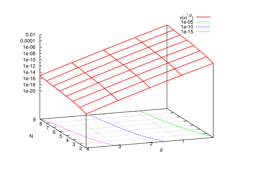
Figure 1:

degree d	N=2	N=3
0	5.2 E-6	3.0 E-5
1	5.4 E-9	3.1 E-8
2	3.7 E-12	2.0 E-11
3	1.9 E-15	1.9 E-14
4	2.2 E-18	3.9 E-15

Table 1: $v(\boldsymbol{\alpha}^{*,d})$

4.2 Empirical study of the optimization step (Step 2)

The stochastic algorithm converges almost surely to the optimal coefficient $\boldsymbol{\alpha}^{*}$. In this part, we empirically study the convergence rate in terms of the number of steps $\Gamma$ and the choice of the sequence $(\rho_{\gamma})$.

4.2.1 A typical evolution of $(\alpha_{\gamma})$

In this subsection, we consider a swap with two payment dates ($N=2$). We consider the truncation set $\Lambda^{(0)}=\{0,1\}$. The objective is to approximate $\boldsymbol{\alpha}^{*}=(\alpha^{0,*}(-1,0),\alpha^{0,*}(-1,1),\alpha^{0,*}(0,1),\alpha^{1,*}(0,1)).$ In Figure 2, the four parameters $\boldsymbol{\alpha}=(\alpha^{0}(-1,0),\alpha^{0}(-1,1),\alpha^{0}(0,1),\alpha^{1}(0,1))$ evolve according to (13) where the sequence $(\rho_{\gamma},\gamma\geq 1)$ is defined by (20) with $v_{1}=10^{7}$, $v_{2}=1$ and $\beta=1$.

As expected, the sequence $(\boldsymbol{\alpha}_{\gamma})$ converges to $\boldsymbol{\alpha}^{*}$. However, the evolution is quite slow although we have empirically chosen the parameters $v_{1}$, $v_{2}$ and $\beta$ in a favorable way.

In Figure 3, we plot (in violet) $v(\alpha^{0}(-1,0),\alpha^{0}(-1,1),\alpha^{0,*}(0,1),\alpha^{1,*}(0,1))$ as a function of $\alpha^{0}(-1,0)$ and $\alpha^{0}(-1,1)$. We also plot in green the path $(v(\boldsymbol{\alpha}_{\gamma}),0\leq\gamma\leq\Gamma)$. The figure shows that after $\Gamma=10000$ steps the hedging error is small though the optimal parameters have not been approximated accurately (notice that the violet surface is flat).

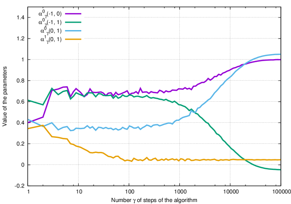
Figure 2: Evolution of the parameters $\alpha^{0}_{\gamma}(-1,0)$, $\alpha^{0}_{\gamma}(-1,1)$, $\alpha^{0}_{\gamma}(0,1)$, $\alpha^{1}_{\gamma}(0,1)$ in terms of $\gamma$.

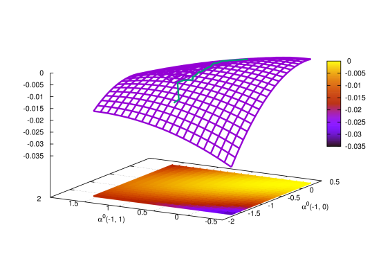
Figure 3: Violet surface: $-v(\centerdot,\centerdot,\alpha^{0,*}(0,1),\alpha^{1,*}(0,1))$. Green curve: evolution of $(\alpha^{0}\gamma(-1,0),\alpha^{0}_{\gamma}(-1,1),-v(\alpha^{0}_{\gamma}(-1,0),\alpha^{0}_{\gamma}(-1,1),\alpha^{0,*}(0,1),\alpha^{1,*}(0,1))$ in terms of $\gamma=1,\cdots,10000$ ($v_{1}=10$, $v_{2}=1$ and $\beta=0.6$).

4.2.2 Sensitivity to the choice of the sequence $(\rho_{\gamma})$

Theorem 4 states the convergence of the optimization method for all sequence $(\rho_{\gamma})$ satisfying (A2). We here study the sensitivity of the results to the parameters $v_{1}$, $v_{2}$, $\beta$ of sequences of type (20) and to the total number of steps $\Gamma$.

Tables 2 and 3 show the expected value function obtained after $\Gamma=10E4$, $10E5$ and $10E6$ steps. The expected value function is estimated by means of a classical Monte Carlo procedure. Table 4 shows the same results with a sequence $\rho_{\gamma}=v_{1}$ which does not satisfy condition (A2).

	1	10	100	1000	10 000	20 000	10E5	10E6
10E4	7.2 E-4	2.6 E-6	1.1 E-6	8.9 E-7	5.1 E-4	8.3 E-4	1.0 E-1	1.3 E-1
10E5	1.4 E-5	9.3 E-7	8.9 E-7	4.7 E-7	2.3 E-8	1.7 E-2	9.1 E+3	9.5 E+5
10E6	3.8 E-6	9.2 E-7	7.7 E-7	1.5 E-7	6.6 E-12	5.4 E-12	1.0 E-5	15.8

Table 2: $v(\boldsymbol{\alpha}_{\Gamma})$ ($v_{2}=1000$, $\mathbf{\beta=0.6}$)

	1	10	100	1000	10 000	13 000	2E4
10E4	8.8 E-3	1.0 E-3	7.8 E-6	9.8 E-7	8.8 E-7	1.7 E-6	9.7 E-7
10E5	6.6 E-3	1.1 E-4	9.3 E-7	9.0 E-7	6.8 E-7	5.5 E-7	4.8 E-7
10E6	4.5 E-3	1.8 E-5	9.3 E-7	8.7 E-7	5.1 E-7	3.6 E-7	2.9 E-7

	1E5	5E5	1E6	2E6	3E6	4E6	5E6
10E4	1.3 E-3	3.3 E-2	7.3 E-1	4.5 E+1	1.1 E-2	6.5 E+2	6.9 E+1
10E5	6.6 E-7	1.2 E-5	4.1 E-4	2.7 E-1	8.1 E-3	1.7 E-2	1.4 E+1
10E6	6.8 E-8	1.1 E-10	5.3 E-12	7.4 E-12	7.0 E-12	2.6 E-5	1.5 E-6

Table 3: $v(\boldsymbol{\alpha}_{\Gamma})$ ($v_{2}=1000$, $\mathbf{\beta=0.9}$)

	1	2	4	6	8	10	12	20
10E4	7.6 E-7	6.9 E-7	2.5 E-7	2.9 E-7	1.4 E-6	1.9 E-7	7.6 E-7	6.1 E-6
10E5	6.9 E-7	6.8 E-7	4.1 E-7	1.3 E-7	2.9 E-7	3.2 E-7	3.9 E-6	3.2 E-4
10E6	3.0 E-8	1.0 E-9	5.1 E-12	4.3 E-12	5.1 E-12	4.2 E-12	5.9 E-12	7.8 E-6

Table 4: $v(\boldsymbol{\alpha}_{\Gamma})$ for a constant sequence $\rho_{\gamma}=v_{1}$

We observe that the efficiency of the algorithm depends on the choice of the parameters $v_{1}$, $v_{2}$, $\beta$ and is really sensitive to it when the total number of steps $\Gamma$ is small.

When $\Gamma$ becomes large (e.g $\Gamma=10E6$), then the algorithm may seem to diverge if $\beta$ is chosen carelessly. In fact, as the sequence $(\rho_{\gamma},\gamma\geq 1)$ satisfies hypothesis (A2) of Theorem 4, the algorithm converges to the optimal parameters but it is far from $\boldsymbol{\alpha}^{*}$ after $10E6$ steps. However, for each value $\beta$, some $v_{1}$ reduces the mean square hedging error to 5 E-12.

5 An empirical study of the bid-ask spread costs impact

We here present numerical results corresponding to two piecewise linear liquidity cost functions $\Psi$:

$$\Psi^{1}_{\lambda}(T,U,\pi) =(1+\lambda\,\text{sign}(\pi))B(T,U)\pi$$ (28)

$$\Psi^{2}_{\lambda,C}(T,U,\pi) =\begin{cases}B(T,U)\pi\mbox{ for }|\pi|\leq C\\ B(T,U)(C+(1+\lambda)(\pi-C)\mbox{ for }\pi>C\\ B(T,U)(-C+(1-\lambda)(\pi+C)\mbox{ for }\pi<-C.\end{cases}$$ (29)

Despite the fact that we know there is no perfect hedging strategy in this context, we suppose the holder receives a null cash at time $t$ (which is the price of the swap in a no liquidity cost market).

We now shortly check the convergence of the algorithm. Given piecewise linear cost functions $\Psi$, it is easy to prove that the terminal wealth $W^{(\boldsymbol{\alpha})}$ is piecewise linear in $\boldsymbol{\alpha}$ (see the proof of proposition 5). Therefore, assumption (A1) of Theorem 4. However, Theorem 4 does not apply to our context since $\Psi^{1}_{\lambda}$ and $\Psi^{2}_{\lambda}$ are piecewise linear and therefore are not continuously differentiable everywhere. Replace $\Psi^{1}_{\lambda}$ and $\Psi^{2}_{\lambda}$ by smooth approximations obtained by convolutions with kernels of the type $1/\sqrt{2\pi\varepsilon}\exp(-x^{2}/(2\varepsilon))$, $\varepsilon$ small. Let $\boldsymbol{\alpha}^{*}_{\varepsilon}$ be the unique optimal parameter corresponding to the new cost functions (existence and uniqueness of $\boldsymbol{\alpha}^{*}_{\varepsilon}$ are provided by Theorem 4). In view of Rockafellar and Wets (1998, Th 7.33) $(\boldsymbol{\alpha}^{*}_{\varepsilon})$ tends to $\boldsymbol{\alpha}^{*}$ when $\varepsilon$ tends to $0$.

The preceding consideration to prove convergence is more theoretical than practical: in practice, the numerical results do not differ when $\varepsilon$ is small or $\varepsilon$ is null.

Finaly, notice that the piecewise linearity in $\boldsymbol{\alpha}$ of $W^{(\boldsymbol{\alpha})}$ implies that conditions in Remark 7 are satisfied, so that Theorem 6 precises the convergence rate.

5.1 Taking liquidity costs into account is really necessary

Consider two different strategies: (i) the strategy corresponding to the optimal parameters $\boldsymbol{\alpha}_{0}$ in the idealistic model without liquidity costs and (ii) the null strategy $\boldsymbol{\delta}_{0}$ defined as

$$\boldsymbol{\delta}_{0}^{\boldsymbol{n}_{(j)}}(j,i)=0,\quad\mbox{ for all }-1\leq j<i\leq N-1\mbox{ and }\boldsymbol{n}_{(j)}\in\Lambda^{(j)}.$$

To satisfy the self-financing assumption (5), at time $T_{j}$ the payoff $P(j)$ of the swap (2) is used to buy zero-coupon bonds with maturity $T_{N}$.

Figure 4 shows $-v(\boldsymbol{\alpha}_{0})$ and $-v(\boldsymbol{\delta}_{0})$ in terms of the parameter $\lambda$ where the cost function $\Psi$ is as in (28). The mean square hedging error dramatically increases when, in the presence of liquidity costs, the trader uses the strategy which is optimal in the no liquidity cost context. When the liquidity cost $\lambda$ is larger than $4\%$, it is even worse to use this strategy than to use the $\boldsymbol{\delta}_{0}$ strategy!

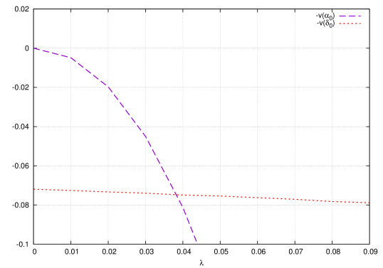
Figure 4: (short dashes) $-v(\boldsymbol{\delta}_{0})$ (long dashes) $-v(\boldsymbol{\alpha}_{0})$ in terms of the liquidity cost $\lambda$

5.2 Probability distribution of the hedging error in the case (28)

In this section, the liquidity cost function $\Psi$ is chosen as in (28).

After $\Gamma$ steps of the stochastic optimization procedure with a sample $\omega$ of the Gaussian vector $((G^{(0)}_{\gamma},\cdots,G^{(N)}_{\gamma}),\gamma=1,\cdots,\Gamma)$, one obtains a random approximation $\boldsymbol{\alpha}_{\Gamma}(\omega)$ of the optimal parameter $\boldsymbol{\alpha}^{*}$.

Figure 5 shows the probability distribution of the random variable $v(\boldsymbol{\alpha}_{\Gamma}(\omega))$ for $\Gamma=10000$ and Table 5 shows its mean and standard deviation for different values of $\lambda$.

$\lambda$	0	0.01	0.02	0.03	0.04	0.05	0.06	0.07	0.08	0.09
Mean	2.5E-32	0.0031	0.012	0.024	0.038	0.049	0.058	0.065	0.11	0.12
Std dev.	6.7E-33	4.2E-5	2.8E-4	1.7E-3	0.016	0.017	0.046	0.081	1.1	1.3

Table 5: Empirical mean and standard deviation of $v(\boldsymbol{\alpha}_{10000})$.

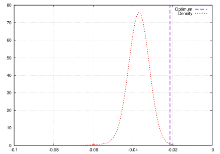
Figure 5: Empirical density of $-v(\boldsymbol{\alpha}_{\Gamma}(\omega))$ ($v_{1}=v_{2}=\beta=1$, $\Gamma=10000$, $\lambda=0.04$). The vertical line corresponds to the $v(\boldsymbol{\alpha}^{*})$.

5.3 Hedging error in the case (29)

In this section, the liquidity cost function $\Psi$ is chosen as in (29).

Figure 6 shows $-v(\boldsymbol{\alpha}_{\Gamma})$ for $\Gamma=0$ (green) and $\Gamma=10E6$ (violet). The initial parameter $\boldsymbol{\alpha}_{0}$ is the optimal one for a market without liquidity cost.

We observe that the main part of the loss is saved thanks to the optimization procedure. In Figure 7, we zoom on the surface resulting from the optimization procedure. Notice that the cost function (28) is equal to the cost function (29) in the particular case $C=0$. So, Figure 7 allows to compare the value functions corresponding to these two cost functions.

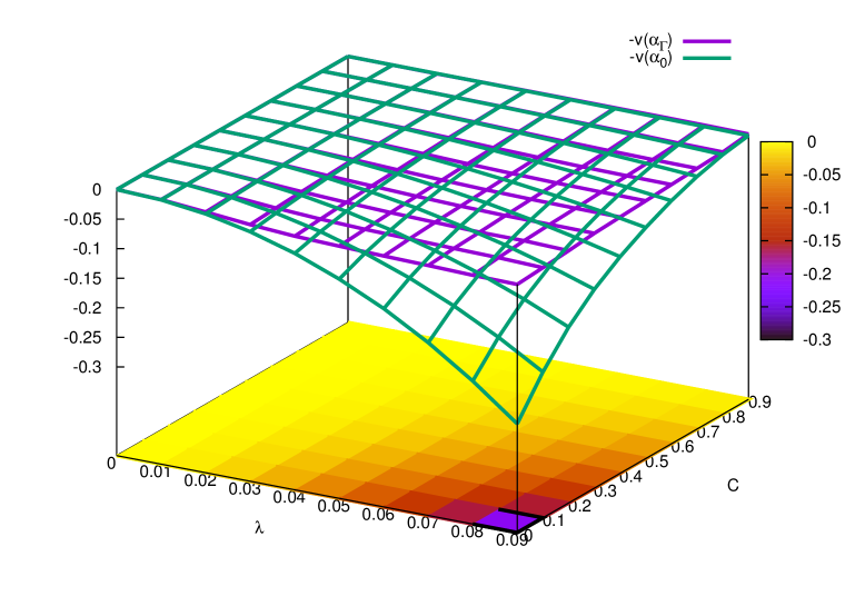
Figure 6: Violet surface: $-v(\boldsymbol{\alpha}_{\Gamma})$ ($\Gamma=10E6$, $v_{1}=v_{2}=100$, $\beta=0.6$) for a liquidity cost function (29) in terms of the value $\lambda$ of the liquidity cost and the size $C$ of the compact. Green surface:$-v(\boldsymbol{\alpha}_{0})$.

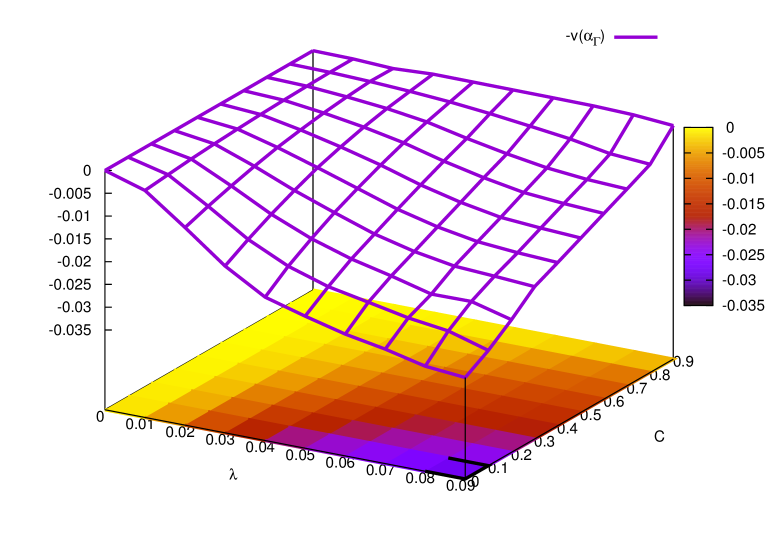
Figure 7: A zoom on the violet surface of Figure 6

5.4 Influence of the initial value $\boldsymbol{\alpha}_{0}$ of the optimization procedure

In Figure 8, we draw two functions of the liquidity cost $\lambda$: $-v(\boldsymbol{\alpha}_{\Gamma})$ and $-v(\boldsymbol{\delta}_{\Gamma})$, where $(\boldsymbol{\alpha}_{\Gamma})$ and $(\boldsymbol{\delta}_{\Gamma})$ are the parameters obtained after $\Gamma$ steps of the optimization procedure but with different initial values $\boldsymbol{\alpha}_{0}$ and $\boldsymbol{\delta}_{0}$ as described in Subsec. 5.1. The performance of the strategies obtained after $\Gamma=10E6$ steps are quite similar. It means that the sensitivity to the arbitrary initial parameter $\boldsymbol{\alpha}_{0}$ is not observable any more after $\Gamma=10E6$ steps.

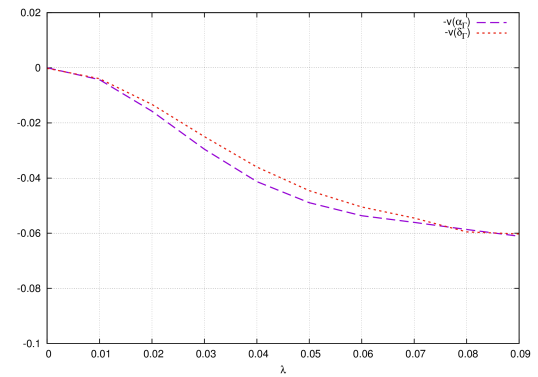
Figure 8: (short dashes) $-v(\boldsymbol{\delta}_{\Gamma})$ (long dashes) $-v(\boldsymbol{\alpha}_{\Gamma})$, in terms of the liquidity cost $\lambda$ ($\Gamma=10E6$, $v_{1}=0.1$, $v_{2}=100$, $\beta=0.6$, $d=3$).

5.5 Reducing the set of admissible strategies

Recall Hypothesis 2. So far, our admissible strategies at time $T_{j}$ depend on all the past and present rates $R_{t},\cdots,R_{T_{j}}$. Thus the number of parameters $\alpha^{\boldsymbol{n}_{(j)}}(j,i)$ to optimize is at least of the order of magnitude of the binomial coefficient $\binom{N}{d}$, where $N$ is the number of dates and the degree of truncation $d$ is defined as in (26). This order of magnitude is a drastically increasing function of $N$. This crucial drawback leads us to try to simplify the complexity of the control problem (6) by reducing the size of the set of the admissible strategies $\Pi$. Observe that the optimal strategy under the perfect liquidity assumption has the property that $\pi^{*}(j,i)$ only depends on $R_{T_{j}}$. This observation suggests to face large numbers of dates by reducing the set of controls to controls depending only on a small number of recent interest rates $R_{T_{j}},R_{T_{j-1}},\cdots,R_{T_{j-q}}$.

Figures 9 and 10 illustrate that the optimal control problem (6) with admissible

strategies defined as in hypothesis 2 may be used as benchmarks to solve control problems. Consider swaps with $N=5$ and $N=10$ dates of payment. In each one of these two cases, we study the effect of choosing $q=0$ (that is at time $T_{j}$, admissible strategies only depend on $R_{T_{j}}$), $q=1$ (admissible strategies depend on $R_{T_{j}}$ and $R_{T_{j-1}}$), $q=2$.

Figure 9 shows the performance of the corresponding strategies obtained after $\Gamma=10E6$ steps of the optimization algorithm for a swap with $N=5$ dates of payments.

Figure 10 shows similar quantities for a swap with $N=10$ dates of payment. We observe that the numerical computation of the optimal strategy is quite unstable when $q$ is too big, which reflects the difficulty to solve a high dimensional optimization problem. Therefore, one necessarily must choose $q$ small in order to get accurate approximations of optimal strategies belonging to reduced sets of admissible strategies.

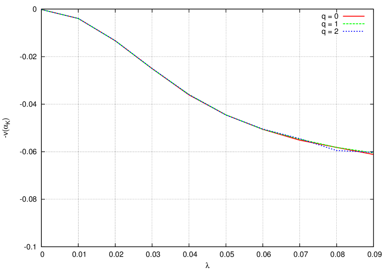
Figure 9: $-v(\boldsymbol{\alpha}_{\Gamma})$ in terms of $\lambda$ for strategies depending only on recent rates $R_{T_{j}},\cdots,R_{T_{j-q}}$ ($q=0,1,2$, $\Gamma=10E6$, $v_{1}=0.1$, $v_{2}=100$, $\beta=0.6$, $d=3$) for a swap with $N=5$ dates of payment.

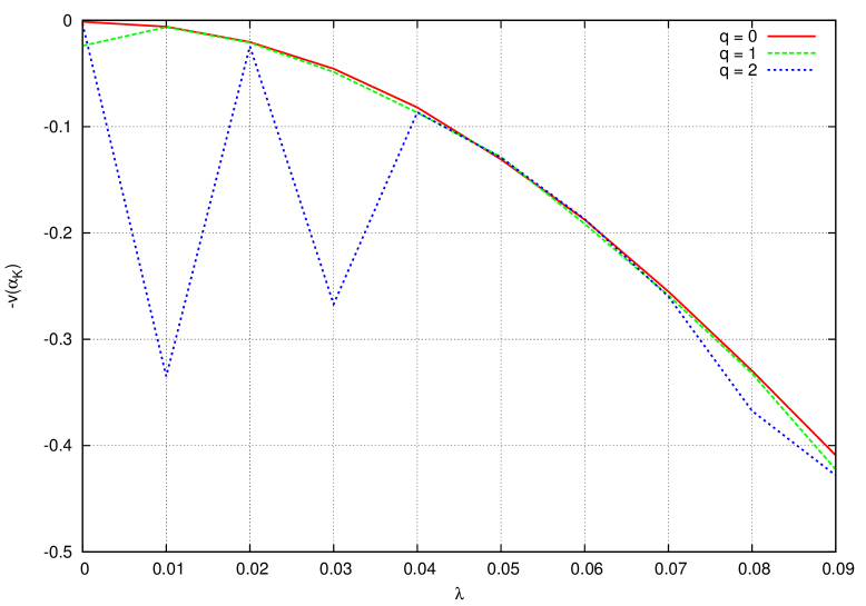
Figure 10: $-v(\boldsymbol{\alpha}_{\Gamma})$ in terms of $\lambda$ for strategies depending only on recent rates $R_{T_{j}},\cdots,R_{T_{j-q}}$ ($q=0,1,2$, $\Gamma=10E6$, $v_{1}=0.1$, $v_{2}=100$, $\beta=0.6$, $d=3$) for a swap with $N=10$ dates of payment.

6 Conclusion

Stochastic control problems generally have no explicit solutions and are difficult to solve numerically. In this paper, we have proposed an efficient algorithm to approximate optimal allocation strategies to hedge interest rate derivatives subject to liquidity costs.

As discussed above, our methodology is constructive and efficient in a Gaussian paradigm. We project the admissible allocation strategies to the space generated by the first Hermite polynomials and use a classical stochastic algorithm to optimally choose the coefficients of the projection in order to optimize an expected function of the terminal hedging error.

We have illustrated this general approach by studying swaps in the presence of liquidity costs. We have discussed the performances of the numerical method in terms of all its algorithmic components.

We emphasize that our methodology can be applied to many control problems, e.g., the computation of indifference prices, when the model under consideration belongs to a Gaussian space.

7 Appendix

Proof of Lemma 9

Proof.

Let us first prove the result for $M=0$, that is $X=\exp\left(\mu+\lambda G\right).$

$$X =\sum_{n=0}^{+\infty}\alpha(n)\dfrac{H_{n}(G)}{\sqrt{n!}}$$

where

$$\alpha(n) =\mathbb{E}\left[X\dfrac{H_{n}(G)}{\sqrt{n!}}\right]=\exp(\mu)\mathbb{E}\left[\exp(\lambda G)\dfrac{H_{n}(G)}{\sqrt{n!}}\right].$$

We then use the identity: $e^{\lambda x-\lambda^{2}/2}=\sum_{j\geqslant 0}\frac{\lambda^{j}}{j!}H_{j}\left(x\right)$ and obtain

$$\alpha(n) =\exp(\mu+\lambda^{2}/2)\mathbb{E}\left[\sum_{j}\dfrac{\lambda^{j}}{j!}H_{j}(G)\dfrac{H_{n}(G)}{\sqrt{n!}}\right].$$

As $(H_{j}(G)/\sqrt{j!},j\geq 0)$ is an orthonormal basis of $L^{2}(G)$ we have

$$\alpha(n)=\exp(\mu+\lambda^{2}/2)\dfrac{\lambda^{n}}{\sqrt{n!}}.$$

Let $X^{d}$ be the projection of $X$ on the subspace generated by the $H_{0},\cdots,H_{d}$ :

$$X^{d} =\sum_{n=0}^{d}\alpha(n)\dfrac{H_{n}(G)}{\sqrt{n!}}=e^{\mu+\lambda^{2}/2}\sum_{n=0}^{d}\dfrac{\lambda^{n}}{\sqrt{n!}}\dfrac{H_{n}(G)}{\sqrt{n!}}$$

$$X-X^{d} =e^{\mu+\lambda^{2}/2}\sum_{n=d+1}^{\infty}\dfrac{\lambda^{n}}{\sqrt{n!}}\dfrac{H_{n}(G)}{\sqrt{n!}}.$$

The truncation error is

$$\|X-X^{d}\|^{2}_{2} =e^{2\mu+\lambda^{2}}\sum_{n=d+1}^{\infty}\dfrac{\lambda^{2n}}{n!}$$

$$\leq e^{2\mu+\lambda^{2}}\dfrac{\lambda^{2(d+1)}}{(d+1)!}\sum_{n=0}^{\infty}\dfrac{\lambda^{2n}}{n!}$$

$$\leq e^{2\mu+2\lambda^{2}}\dfrac{\lambda^{2(d+1)}}{(d+1)!}.$$

The desired result thus holds true for $M=0$. Let $M$ be a positive integer. We have

$$\|X-X^{d}\|^{2}_{2}=e^{2\mu+\lambda_{0}^{2}+\cdots+\lambda_{M}^{2}}\sum_{n_{0}+\cdots+n_{M}>d}\prod_{m=0}^{M}\dfrac{\lambda_{m}^{2n_{m}}}{(n_{m})!}$$

Recall the classical identity

$$\dfrac{\left(a_{0}+\cdots+a_{L}\right)^{N}}{N!}=\sum_{n_{0}+\cdots+n_{L}=N}\prod_{m=0}^{L}\dfrac{a_{m}^{n_{m}}}{(n_{m})!}.$$ (30)

Thus,

$$\sum_{n_{0}+\cdots+n_{M}>d}\prod_{m=0}^{M}\dfrac{\lambda_{m}^{2n_{m}}}{(n_{m})!} =\sum_{N=d+1}^{\infty}\sum_{n_{0}+\cdots+n_{M}=N}\prod_{m=0}^{M}\dfrac{\lambda_{m}^{2n_{m}}}{(n_{m})!}$$

$$=\sum_{N=d+1}^{\infty}\dfrac{\left(\lambda_{0}^{2}+\cdots+\lambda_{M}^{2}\right)^{N}}{N!}$$

$$\leq\dfrac{\left(\lambda_{0}^{2}+\cdots+\lambda_{M}^{2}\right)^{d+1}}{(d+1)!}\exp\left(\lambda_{0}^{2}+\cdots+\lambda_{M}^{2}\right).$$

This ends the proof for all positive $M$. ∎

References

- Babbs and Nowman (1999) Babbs, S. H. and Nowman, K. B. (1999) Kalman Filtering of Generalized Vasicek Term Structure Models, Journal of Financial and Quantitative Analysis, 34(1), pp. 115–130.
- Chen (2002) Chen, H. F. (2002) Stochastic Approximation and its Applications, Nonconvex Optimization and its Applications Vol. 64 (Kluwer Academic Publishers, Dordrecht).
- Chen and Zhu (1986) Chen, H. F. and Zhu, Y. (1986) Stochastic approximation procedures with randomly varying truncations, Sci. Sinica Ser. A, 29(9), pp. 914–926.
- Dai and Singleton (2000) Dai, Q. and Singleton, K. J. (2000) Analysis of Affine Term Structure Models, The Journal of Finance, 55(5), pp. 1943–1978.
- Duflo (1997) Duflo, M. (1997) Random Iterative Models, Applications of Mathematics (New York) Vol. 34 (Springer-Verlag, Berlin).
- Gibson et al. (2010) Gibson, R., Lhabitant, F. S. and Talay, D. (2010) Modeling the Term Structure of Interest Rates: A Review of the Literature, Foundations and Trends in Finance Vol. 5(1-2) (Now Publisher).
- Kushner and Yin (2003) Kushner, H. J. and Yin, G. G. (2003) Stochastic Approximation and Recursive Algorithms and Applications, Second, Applications of Mathematics (New York) Vol. 35 (Springer-Verlag, New York) Stochastic Modelling and Applied Probability.
- Lelong (2008) Lelong, J. (2008) Almost sure convergence for randomly truncated stochastic algorithms under verifiable conditions, Statist. Probab. Lett., 78(16), pp. 2632–2636.
- Lelong (2013) Lelong, J. (2013) Asymptotic normality of randomly truncated stochastic algorithms, ESAIM Probab. Stat., 17, pp. 105–119.
- Malliavin (1995) Malliavin, P. (1995) Integration and Probability, Graduate Texts in Mathematics Vol. 157 (New York: Springer-Verlag).
- Musiela and Rutkowski (2005) Musiela, M. and Rutkowski, M. (2005) Martingale methods in financial modelling, Second, Stochastic Modelling and Applied Probability Vol. 36 (Springer-Verlag, Berlin).
- Robbins and Monro (1951) Robbins, H. and Monro, S. (1951) A stochastic approximation method, Ann. Math. Statistics, 22, pp. 400–407.
- Rockafellar and Wets (1998) Rockafellar, R. T. and Wets, R. J. B. (1998) Variational analysis, Grundlehren der Mathematischen Wissenschaften [Fundamental Principles of Mathematical Sciences] Vol. 317 (Springer-Verlag, Berlin).