Neutron star equations of state with optical potential constraint

Abstract

Nuclear matter and neutron stars are studied in the framework of an extended relativistic mean-field (RMF) model with higher-order derivative and density dependent couplings of nucleons to the meson fields. The derivative couplings lead to an energy dependence of the scalar and vector self-energies of the nucleons. It can be adjusted to be consistent with experimental results for the optical potential in nuclear matter. Several parametrisations, which give identical predictions for the saturation properties of nuclear matter, are presented for different forms of the derivative coupling functions. The stellar structure of spherical, non-rotating stars is calculated for these new equations of state (EoS). A substantial softening of the EoS and a reduction of the maximum mass of neutron stars is found if the optical potential constraint is satisfied.

1 Introduction

The recent observation of two pulsars with approximately two solar masses [1, 2] presents a severe challenge to the theoretical description of cold high-density matter in $\beta$-equilibrium. The equation of state (EoS) has to be sufficiently stiff in order to support such high masses of compact stars. Many models that are solely based on nucleonic (neutrons and protons) and leptonic (electrons and muons) degrees of freedom are able to reproduce maximum neutron star masses above two solar masses if the effective interaction between the nucleons becomes strongly repulsive at high baryon densities. However, additional hadronic particle species can appear at densities above two or three times the nuclear saturation density $n_{\rm sat}\approx 0.16$ fm^-3. In most cases, these additional degrees of freedom lead to a substantial softening of the EoS resulting in a reduced maximum mass of the compact star below the observed values. This feature is well-known for models with hyperons – the so-called ”hyperon puzzle”, see, e.g., [3, 4] and references therein – but was also observed in approaches that take excited states of the nucleons such as $\Delta(1232)$ resonances into account, see, e.g., [5, 6] and references therein. Usually, only specifically designed interactions can avoid the problem of too low maximum masses.

Successful models of the baryonic contribution to the stellar EoS should be scrutinized whether they comply with other experimental constraints, e.g. with respect to the employed interactions. In the center of compact stars very high baryon densities are reached exceeding several times $n_{\rm sat}$ and the corresponding Fermi momenta of the particles are much larger than those at saturation. This is particularly significant for models with only nucleonic degrees of freedom. Hence, not only the density dependence of the effective in-medium interaction between nucleons but also their momentum dependence becomes relevant. For densities near $n_{\rm sat}$ this information is contained in the optical potential of nucleons that can be extracted from the systematics of elastic proton scattering on nuclei, see, e.g., [7, 8]. A saturation of the real part of the optical potential is observed at high kinetic energies approaching $1$ GeV. The momentum dependence of the in-medium interaction is also crucial in simulations of heavy-ion collisions [9].

Typical approaches for the baryonic contribution to the stellar EoS are energy density functionals that originate from nonrelativistic or relativistic mean-field models of nuclear matter. The most prominent cases among the former class are Skyrme energy density functionals, see reference [10] for an overview of different parametrizations. They are derived originally from the zero-range Skyrme interaction with a two-body contribution, which is an expansion up to second order in the particle momenta, and a density dependent three-body contribution, which is included in order to reproduce saturation properties of nuclear matter. Obviously, an extrapolation of the model to high momenta is questionable given the limited form of the momentum dependence. Examples of the latter class, frequently denominated covariant density functionals, can be inferred from relativistic Lagrangian densities. In conventional models, see reference [11] for a wide collection of different parametrizations, a nucleon optical potential in the medium can be derived from the relativistic scalar and vector self-energies, see section 5. It exhibits a linear increase with energy, which is in contradiction with the expectation from experiment. In general, one would expect that the nucleon self-energies itself depend explicitly on the particle momentum or energy as, e.g., in Dirac-Brueckner calculations of nuclear matter [12]. However, this is not realized in standard RMF models.

There are particular extensions of relativistic mean-field (RMF) models that contain nucleon self-energies with an explicit energy or momentum dependence. This dependence cannot be introduced in a relativistic model in a simple parametric form because it affects, e.g., the definition of the conserved currents. In extended systematic approaches new derivative couplings between the nucleon and meson fields are introduced that allow to reproduce the energy dependence of the optical potential as extracted from experiments. One of the earliest RMF models with scalar derivative couplings was presented in reference [13]. A rescaling of the nucleon fields removed the explicit momentum dependence of the self-energies but lead to a considerable softening of the EoS. More general couplings of the mesons to linear derivatives of the nucleon fields were considered in reference [14] with an application to uniform nuclear matter. With appropriately chosen coupling constants a reduction of the optical potential was found as compared to the strong linear energy dependence in conventional RMF models. The model was further extended in reference [15] assuming a density dependence of the couplings. It was successfully applied to the description of finite nuclei. Notable new features were the increase of the effective nucleon masses (usually rather small in order to explain the strong spin-orbit interaction in nuclei) and correspondingly higher level densities close to the Fermi energy in nuclei in better concordance with expectations from experiments. Though, using couplings only linear in the derivatives leads to a quadratic dependence of the optical potential on the kinetic energy with a decrease for energies exceeding $1$ GeV. Couplings to all orders in the derivative of the nucleons were introduced in the so-called nonlinear derivative (NLD) model [16, 17] assuming a particular exponential dependence on the derivatives but no density dependence of the nucleon-meson couplings or self-couplings of the mesons. The general formalism was developed and applied to infinite isospin symmetric and asymmetric nuclear matter with a particular choice of the non-linear derivative terms that lead to an energy dependence of the self-energies. In reference [18] the approach was extended with generalized non-linear derivative couplings of any functional form in the field-theoretical formalism allowing for a momentum or energy dependence. Nonlinear self-couplings of the $\sigma$ meson field were added in order to improve the description of characteristic nuclear matter parameters at saturation. The application of this version of the NLD model to stellar matter yielded a maximum neutron star mass of $2.03~{}M_{\rm sol}$ barely satisfying the observational constraints but the dependence of the result on the model parameters was not explored in detail. The NLD model was also applied to the description of bulk properties of nuclear matter in reference [19]. A softening of the EoS and maximum masses of neutron stars substantially below $2~{}M_{\rm sol}$ were found with different parametrizations assuming an energy dependence of the couplings but nonlinear self-couplings of the mesons or density dependent meson-nucleon couplings were not considered. Properties of finite nuclei were studied in reference [20] after adding meson self-interactions in the Lagrangian. A qualitative description similar to conventional RMF models was achieved but neutron star properties were not examined in this extended model.

In this work we introduce a more flexible extension of the nonlinear derivative model assuming density dependent meson-nucleon couplings in addition. Instead of using derivative operators that generate an explicit momentum dependence of the self-energies, we will use a functional form that leads to an energy dependence. This approach will also be more suitable for a future applications of the DD-NLD approach to nuclei since the relevant equations and their numerical implementation are simplified. Here, the equations of state of symmetric and asymmetric nuclear matter will be calculated for different choices of the derivative coupling operators that lead to a saturation of the optical potential at high energies as derived from experiments. They are compared to the results of a standard RMF model with density dependent couplings that is consistent with essentially all modern constraints for the characteristic nuclear matter parameters at saturation. The parameters of the DD-NLD models are chosen such that these saturation properties are reproduced. The effect of the optical potential constraint on the mass-radius relations of neutron stars will be studied.

The paper is organized as follows: In section 2 the Lagrangian density of the DD-NLD approach is presented. The field equations in mean-field approximation and the energy-momentum tensor will be derived. The relevant equations for the case of infinite nuclear matter will be considered in more detail in section 3. The parametrization of the density dependent couplings and the functional form of the derivative coupling functions is discussed in section 4. Results for the energy dependence of the optical potential, the EoS of nuclear matter and the mass-radius relation are presented in section 5 for various versions of the model. Conclusions are given in section 6. Detailed expression for various densities are collected in A.

2 Lagrangian density and field equations of the DD-NLD model

In most RMF models the effective interaction between nucleons is described by an exchange of mesons. Usually, $\sigma$ and $\omega$ mesons are introduced to consider the attractive and repulsive contributions to the nucleon-nucleon potential, respectively. They are represented by isoscalar Lorentz scalar and Lorentz vector fields $\sigma$ and $\omega_{\mu}$. In order to model the isospin dependence of the interaction, the exchange of $\rho$ mesons is included. It is denoted by the isovector Lorentz vector field $\bm{\rho}_{\mu}$ in the following. The Lagrangian density in the DD-NLD approach

$$\mathcal{L}=\mathcal{L}_{\rm nuc}+\mathcal{L}_{\rm mes}+\mathcal{L}_{\rm int}$$ (1)

contains contributions of the free nucleons $\Psi=(\Psi_{p},\Psi_{n})$ with mass $m$

$$\mathcal{L}_{\rm nuc}=\frac{1}{2}\left(\overline{\Psi}\gamma_{\mu}i\overrightarrow{\partial^{\mu}}\Psi-\overline{\Psi}i\overleftarrow{\partial^{\mu}}\gamma_{\mu}\Psi\right)-m\overline{\Psi}\Psi$$ (2)

in a symmetrized form and of free mesons

$$\mathcal{L}_{\rm mes} = \frac{1}{2}\left(\partial_{\mu}\sigma\partial^{\mu}\sigma-m^{2}_{\sigma}\sigma^{2}-\frac{1}{2}F^{(\omega)}_{\mu\nu}F^{(\omega)\mu\nu}+m^{2}_{\omega}\omega_{\mu}\omega^{\mu}\right.$$

$$\left.-\frac{1}{2}\bm{F}^{(\rho)}_{\mu\nu}\bm{F}^{(\rho)\mu\nu}+m^{2}_{\rho}\bm{\rho}_{\mu}\bm{\rho}^{\mu}\right)$$

with the field tensors

$$F^{(\omega)}_{\mu\nu}=\partial_{\mu}\omega_{\nu}-\partial_{\nu}\omega_{\mu}\quad\mbox{and}\quad\bm{F}^{(\rho)}_{\mu\nu}=\partial_{\mu}\bm{\rho}_{\nu}-\partial_{\nu}\bm{\rho}_{\mu}$$ (4)

of the isoscalar $\omega$ meson and the isovector $\rho$ meson, respectively. The arrows in equation (2) denote the direction of differentiation.

Standard RMF models assume a minimal coupling of the nucleons to the meson fields leading to

$$\mathcal{L}_{\rm int}=\Gamma_{\sigma}\sigma\overline{\Psi}\Psi-\Gamma_{\omega}\omega_{\mu}\overline{\Psi}\gamma^{\mu}\Psi-\Gamma_{\rho}\bm{\rho}_{\mu}\overline{\Psi}\bm{\tau}\gamma^{\mu}\Psi$$ (5)

for the interaction contribution to the total Lagrangian density $\mathcal{L}$ with meson-nucleon couplings $\Gamma_{i}$ ($i=\sigma,\omega,\rho$). We assume that they depend on the vector density $n_{v}$, see equation (25) for the explicit definition. In the derivative coupling model the nucleon field $\Psi$ ($\overline{\Psi}$) is replaced in $\mathcal{L}_{\rm int}$ by $\mathcal{D}_{m}\Psi$ ($\overline{\mathcal{D}_{m}\Psi}$) with operator functions $\mathcal{D}_{m}$, which can be different for the various mesons $m=\sigma,\omega,\rho$. They can be expanded in a series

$$\mathcal{D}_{m}(x)=\sum_{n=0}^{\infty}\frac{d_{n}^{(m)}}{n!}x^{n}$$ (6)

with numerical coefficients $d_{n}^{(m)}$. The argument $x$ contains derivatives $i\partial_{\beta}$ that act on the nucleon field. More specifically we write

$$x=v^{\beta}i\partial_{\beta}-sm$$ (7)

as a hermitian Lorentz scalar operator with an auxiliary Lorentz vector $v^{\beta}=(v_{0},\vec{v})$ and a scalar factor $s$. Hence the interaction contribution in the NLD model is written as

$$\mathcal{L}_{\rm int} = \frac{1}{2}\Gamma_{\sigma}\sigma\left(\overline{\Psi}\overleftarrow{\mathcal{D}}_{\sigma}\Psi+\overline{\Psi}\overrightarrow{\mathcal{D}}_{\sigma}\Psi\right)$$

$$-\frac{1}{2}\Gamma_{\omega}\omega_{\mu}\left(\overline{\Psi}\overleftarrow{\mathcal{D}}_{\omega}\gamma^{\mu}\Psi+\overline{\Psi}\gamma^{\mu}\overrightarrow{\mathcal{D}}_{\omega}\Psi\right)$$

$$-\frac{1}{2}\Gamma_{\rho}\bm{\rho}_{\mu}\left(\overline{\Psi}\overleftarrow{\mathcal{D}}_{\rho}\gamma^{\mu}\bm{\tau}\Psi+\overline{\Psi}\bm{\tau}\gamma^{\mu}\overrightarrow{\mathcal{D}}_{\rho}\Psi\right)$$

in a symmetrized form with respect to the derivative operators $\mathcal{D}_{m}$, i.e.,

$$\overrightarrow{\mathcal{D}}_{m} = \sum^{\infty}_{k=0}C_{k}^{(m)}(v^{\beta}i\overrightarrow{\partial}_{\beta})^{k}$$ (9)

$$\overleftarrow{\mathcal{D}}_{m} = \sum^{\infty}_{k=0}C_{k}^{(m)}(-v^{\beta}i\overleftarrow{\partial}_{\beta})^{k}$$ (10)

with coefficients

$$C_{k}^{(m)}=\sum^{k}_{n=0}\frac{d_{n}^{(m)}}{n!}\binom{n}{k}(-sm)^{n-k}\>.$$ (11)

Obviously, no derivatives appear for the choice $\mathcal{D}_{m}=1$ (corresponding to $d_{n}^{(m)}=\delta_{n0}$) and the standard form (5) is recovered.

When spatially inhomogeneous systems with Coulomb interaction are considered, $\mathcal{L}_{\rm mes}$ and $\mathcal{L}_{\rm int}$ can be complemented with the appropriate contributions. Since only uniform matter is considered in the following, we do not give them here explicitly.

The field equations of nucleons are derived from the generalized Euler-Lagrange equation

$$\frac{\partial\mathcal{L}}{\partial\varphi_{r}}+\sum^{\infty}_{i=1}(-)^{i}\partial_{\alpha_{1},\dots,\alpha_{i}}\frac{\partial\mathcal{L}}{\partial(\partial_{\alpha_{1},\dots,\alpha_{i}}\varphi_{r})}=0$$ (12)

for $\varphi_{r}=\Psi,\overline{\Psi}$. For the meson fields $\varphi_{r}=\sigma,\omega_{\mu},\bm{\rho}_{\mu}$ the standard Euler-Lagrange equation applies, i.e. only the $i=1$ term in equation (12) is relevant since higher-order derivatives of the meson fields do not appear in the Lagrangian density $\mathcal{L}$.

Details can found in references [16, 18]. The Dirac equation

$$\left[\gamma_{\mu}\left(i\partial^{\mu}-\Sigma^{\mu}\right)-\left(m-\Sigma\right)\right]\Psi=0$$ (13)

for the nucleons looks formally the same as in standard RMF approaches but the scalar ($\Sigma$) and vector ($\Sigma^{\mu}$) self-energy operators now contain the derivative operators $\mathcal{D}_{m}$. They are given by

$$\ \Sigma=\Gamma_{\sigma}\sigma\overrightarrow{\mathcal{D}}_{\sigma}$$ (14)

and

$$\Sigma^{\mu}=\Gamma_{\omega}\omega^{\mu}\overrightarrow{\mathcal{D}}_{\omega}+\Gamma_{\rho}\bm{\tau}\cdot\bm{\rho}^{\mu}\overrightarrow{\mathcal{D}}_{\rho}+\Sigma^{\mu}_{R}$$ (15)

with the ’rearrangement’ contribution

$$\Sigma^{\mu}_{R} = \frac{j^{\mu}}{n_{v}}\left[\Gamma_{\omega}^{\prime}\omega^{\nu}\frac{1}{2}\left(\overline{\Psi}\overleftarrow{\mathcal{D}}_{\omega}\gamma_{\nu}\Psi+\overline{\Psi}\gamma_{\nu}\overrightarrow{\mathcal{D}}_{\omega}\Psi\right)\right.$$

$$\left.+\Gamma_{\rho}^{\prime}\bm{\rho}^{\nu}\frac{1}{2}\left(\overline{\Psi}\overleftarrow{\mathcal{D}}_{\rho}\gamma_{\nu}\bm{\tau}\Psi+\overline{\Psi}\gamma_{\nu}\bm{\tau}\overrightarrow{\mathcal{D}}_{\rho}\Psi\right)\right.$$

$$\left.-\Gamma_{\sigma}^{\prime}\sigma\frac{1}{2}\left(\overline{\Psi}\overleftarrow{\mathcal{D}}_{\sigma}\Psi+\overline{\Psi}\overrightarrow{\mathcal{D}}_{\sigma}\Psi\right)\right]$$

containing derivatives

$$\Gamma_{i}^{\prime}=\frac{d\Gamma_{i}}{dn_{v}}$$ (17)

of the coupling functions. In the case of inhomogeneous systems and a non-vanishing three-vector component $\vec{v}$ of the auxiliary vector $v^{\beta}$, additional contributions in (14) and (15) will appear. In the present application of the DD-NLD model, however, we do not consider this case. The field equations of the mesons are found as

$$\partial_{\mu}\partial^{\mu}\sigma+m^{2}_{\sigma}\sigma = \frac{1}{2}\Gamma_{\sigma}\left(\overline{\Psi}\overleftarrow{\mathcal{D}}_{\sigma}\Psi+\overline{\Psi}\overrightarrow{\mathcal{D}}_{\sigma}\Psi\right)$$ (18)

$$\partial_{\mu}F^{(\omega)\mu\nu}+m^{2}_{\omega}\omega^{\nu} = \frac{1}{2}\Gamma_{\omega}\left(\overline{\Psi}\overleftarrow{\mathcal{D}}_{\omega}\gamma^{\nu}\Psi+\overline{\Psi}\gamma^{\nu}\overrightarrow{\mathcal{D}}_{\omega}\Psi\right)$$ (19)

$$\partial_{\mu}\bm{F}^{(\rho)\mu\nu}+m^{2}_{\rho}\bm{\rho}^{\nu} = \frac{1}{2}\Gamma_{\rho}\left(\overline{\Psi}\overleftarrow{\mathcal{D}}_{\rho}\gamma^{\nu}\bm{\tau}\Psi+\overline{\Psi}\bm{\tau}\gamma^{\nu}\overrightarrow{\mathcal{D}}_{\rho}\Psi\right)$$ (20)

with source terms containing derivative operators.

The conserved baryon current in the DD-NLD model is given by

$$J^{\mu}=\sum_{i=p,n}\langle\overline{\Psi}_{i}N^{\mu}\Psi_{i}\rangle$$ (21)

with the norm operator

$$N^{\mu}=\gamma^{\mu}+\Gamma_{\sigma}\sigma\left(\partial^{\mu}_{p}\mathcal{D}_{\sigma}\right)-\Gamma_{\omega}\omega_{\alpha}\gamma^{\alpha}\left(\partial^{\mu}_{p}\mathcal{D}_{\omega}\right)-\Gamma_{\rho}\bm{\rho}_{\alpha}\gamma^{\alpha}\bm{\tau}\left(\partial^{\mu}_{p}\mathcal{D}_{\rho}\right)$$ (22)

where $\partial^{\mu}_{p}\mathcal{D}_{m}$ is the derivative of $\mathcal{D}_{m}$ operator with respect to the momentum $p_{\mu}=i\partial_{\mu}$, i.e.

$$\partial^{\mu}_{p}\mathcal{D}_{m}=v^{\mu}\sum^{\infty}_{k=1}kC_{k}^{(m)}(v^{\beta}i\partial_{\beta})^{k-1}\>,$$ (23)

and $\langle\dots\rangle$ denotes the summation over all occupied states. The current (21) is not identical to the vector current

$$J_{v}^{\mu}=\sum_{i=p,n}\langle\overline{\Psi}_{i}\gamma^{\mu}\Psi_{i}\rangle\>,$$ (24)

which is used to define the vector density

$$n_{v}=\sqrt{J_{v}^{\mu}J_{v\mu}}$$ (25)

appearing as the argument of the coupling functions $\Gamma_{i}$. The energy-momentum tensor assumes the form

$$T^{\mu\nu}=\sum_{i=p,n}\langle\overline{\Psi}_{i}N^{\mu}p^{\nu}\Psi_{i}\rangle-g^{\mu\nu}\langle\mathcal{L}\rangle\>.$$ (26)

Then the energy density $\varepsilon$ and pressure $p$ are found from $\varepsilon=T^{00}$ and $p=\sum_{i=1}^{3}T^{ii}/3$, respectively.

3 DD-NLD model for nuclear matter

In the case of stationary nuclear matter, the equations simplify considerably since the system is homogeneous and the meson fields, which are treated as classical fields, are constant in space and time. Positive-energy solutions of the Dirac equation (13) are plane waves $\Psi_{i}=u_{i}\exp\left(-ip_{i}^{\mu}x_{\mu}\right)$ for protons and neutrons with Dirac spinors $u_{i}$, which are normalized according to

$$\overline{\Psi}_{i}N^{0}\Psi_{i}=\bar{u}_{i}N^{0}u_{i}=1$$ (27)

with the time component of the norm operator (22). They depend on the effective mass

$$m_{i}^{\ast}=m_{i}-\Sigma_{i}$$ (28)

and effective momentum

$$p_{i}^{\ast\mu}=p_{i}^{\mu}-\Sigma_{i}^{\mu}$$ (29)

related by the dispersion relation

$$p_{i}^{\ast\mu}p_{i\mu}^{\ast}=\left(m_{i}^{\ast}\right)^{2}\>.$$ (30)

The derivative $i\partial^{\beta}$ in the $\mathcal{D}_{m}$ operators can be replaced by the corresponding four-momentum $p_{i}^{\beta}=(E_{i},\vec{p}_{i})$ resulting in a simple function $D_{m}$ depending on the energy $E_{i}$ and the momentum $\vec{p}_{i}$ of the nucleon.

Using the identity

$$N^{\mu}\Psi_{i}=\left[\gamma^{\mu}+\partial_{p}^{\mu}\Sigma_{i}-\gamma_{\alpha}\partial_{p}^{\mu}\left(\Sigma_{i}^{\alpha}-\Sigma_{R}^{\alpha}\right)\right]\Psi_{i}$$ (31)

the conserved current and the energy-momentum tensor can be written as

$$J^{\mu}=\sum_{i=p,n}\kappa_{i}\int\frac{d^{3}p}{(2\pi)^{3}}\>\frac{\Pi^{\mu}_{i}}{\Pi^{0}_{i}}$$ (32)

and

$$T^{\mu\nu}=\sum_{i=p,n}\kappa_{i}\int\frac{d^{3}p}{(2\pi)^{3}}\>\frac{\Pi^{\mu}_{i}p^{\nu}}{\Pi^{0}_{i}}-g^{\mu\nu}\langle\mathcal{L}\rangle\>,$$ (33)

respectively, with the four-momentum

$$\Pi^{\mu}_{i}=p^{\ast\mu}_{i}+m^{\ast}_{i}\left(\partial^{\mu}_{p}\Sigma_{i}\right)-p^{\ast}_{i\beta}\left[\partial^{\mu}_{p}\left(\Sigma^{\beta}_{i}-\Sigma^{\beta}_{R}\right)\right]$$ (34)

and spin degeneracy factors $\kappa_{i}=2$. The integration runs over all momenta $p$ with modulus lower than the Fermi momenta $p_{Fi}$ in the no-sea approximation. They are defined through the individual nucleon densities

$$n_{i}=\frac{\kappa_{i}}{6\pi^{2}}p_{Fi}^{3}\>.$$ (35)

Without the preference for a particular direction in infinite nuclear matter, the spatial components of the Lorentz vector meson fields vanish and the auxiliary vector in equation (7) is set to $v^{\beta}=\delta_{\beta 0}$ such that the $D_{m}$ functions only depend on the nucleon energy $E_{i}$. Without isospin changing processes, only the third component of the isovector $\rho$ field has to be considered in the field equations for the mesons. Using the abbreviations $\omega=\omega^{0}$ and $\rho=\bm{\rho}^{0}_{3}$ the meson fields are immediately obtained from

$$\sigma = \frac{\Gamma_{\sigma}}{m_{\sigma}^{2}}n_{\sigma}=\frac{\Gamma_{\sigma}}{m_{\sigma}^{2}}\sum_{i=p,n}\langle\overline{\Psi}_{i}D_{\sigma}\Psi_{i}\rangle$$ (36)

$$\omega = \frac{\Gamma_{\omega}}{m_{\omega}^{2}}n_{\omega}=\frac{\Gamma_{\omega}}{m_{\omega}^{2}}\sum_{i=p,n}\langle\overline{\Psi}_{i}\gamma^{0}D_{\omega}\Psi_{i}\rangle$$ (37)

$$\rho = \frac{\Gamma_{\rho}}{m_{\rho}^{2}}n_{\rho}=\frac{\Gamma_{\rho}}{m_{\rho}^{2}}\sum_{i=p,n}\langle\overline{\Psi}_{i}\gamma^{0}\tau_{3}D_{\rho}\Psi_{i}\rangle$$ (38)

with source densities $n_{\sigma}$, $n_{\omega}$, and $n_{\rho}$. The self-energies simplify to

$$\Sigma_{i} = \Gamma_{\sigma}\sigma D_{\sigma}$$ (39)

$$\Sigma_{i}^{0} = \Gamma_{\omega}\omega D_{\omega}+\Gamma_{\rho}\tau_{3,i}\rho D_{\rho}+\Sigma^{0}_{R}$$ (40)

$$\vec{\Sigma}_{i} = 0$$ (41)

with $\tau_{3,i}=1$ ($-1$) for protons (neutrons) and the ’rearrangement’ contribution

$$\Sigma^{0}_{R}=\Gamma_{\omega}^{\prime}\omega n_{\omega}+\Gamma_{\rho}^{\prime}\rho n_{\rho}-\Gamma_{\sigma}^{\prime}\sigma n_{\sigma}$$ (42)

is independent of the nucleon energy. The dispersion relation reads

$$E_{i}=\sqrt{p^{2}+\left(m_{i}-S_{i}\right)^{2}}+V_{i}$$ (43)

if we introduce the energy-dependent scalar potentials $S_{i}(E)=\Sigma_{i}$ and vector potentials $V_{i}(E)=\Sigma_{i}^{0}$. Explicit expressions for the various densities and thermodynamic quantities of the DD-NLD model are given in A.

4 Parametrization of the DD-NLD model

For the application of the DD-NLD model to nuclear matter the parameters need to be specified. Besides the usual parameters of a RMF model with density dependent couplings the form of the $D_{m}$ functions has to be given. We assume identical functions for all mesons, i.e. $D=D_{\sigma}=D_{\omega}=D_{\rho}$, and consider three functional dependencies:

• a constant $D=1$, which corresponds to a usual RMF model with density dependent couplings,

• a Lorentzian form $D=1/(1+x^{2})$,

• an exponential dependence $D=\exp\left(-x\right)$

with $x=(E_{i}-m_{i})/\Lambda$ because we set $v^{\beta}=\delta_{\beta 0}$ and $s=1$ in equation (7). The parameter $\Lambda$ regulates the strength of the energy dependence. For the proton and neutron masses the experimental values of $m_{p}=938.272046$ MeV/c² and $m_{n}=939.565379$ MeV/c², respectively, are used. The meson masses are set to $m_{\sigma}=550$ MeV/c², $m_{\omega}=783$ MeV/c², and $m_{\rho}=763$ MeV/c². The density dependence of the meson nucleon couplings has the same form as introduced in reference [21]. We assume a dependence on the vector density $n_{v}$ as defined in equation (25), which is not identical to the zero-component of the conserved baryon current (21). See A for explicit expressions. This choice simplifies the rearrangement terms considerably.

For the isoscalar mesons $m=\sigma,\omega$ the coupling is written as

$$\Gamma_{m}(n_{v})=\Gamma_{m}(n_{\rm ref})f_{m}(x)$$ (44)

with functions

$$f_{m}(x)=a_{m}\frac{1+b_{m}(x+d_{m})^{2}}{1+c_{m}(x+d_{m})^{2}}$$ (45)

that depend on the argument $x=n_{v}/n_{\rm ref}$ and contain coefficients $a_{m}$, $b_{m}$, $c_{m}$, and $d_{m}$. For the $\rho$-meson coupling we set

$$\Gamma_{\rho}(n_{v})=\Gamma_{\rho}(n_{\rm ref})\exp\left[-a_{\rho}\left(x-1\right)\right]\>.$$ (46)

In order to reduce the number of independent parameters we demand that the conditions $f_{\sigma}(1)=f_{\omega}(1)=1$ and $f_{\sigma}^{\prime\prime}(0)=f_{\omega}^{\prime\prime}(0)=0$ hold. Hence, there are only two independent coefficients in the functions $f_{m}$ for each of the isoscalar mesons. The overall magnitude of the couplings is given by the couplings $\Gamma_{m}(n_{\rm ref})$ at a reference density $n_{\rm ref}$. We require that the characteristic saturation properties for the three choices of the $D$ function are identical and close to current values extracted from experiments. In particular, we set the saturation density to $n_{\rm sat}=0.15$ fm^-3, the binding energy per nucleon at saturation to $B=16$ MeV, the compressibility to $K=240$ MeV, the symmetry energy to $J=32$ MeV and the symmetry energy slope coefficient to $L=60$ MeV. Furthermore, we set the effective nucleon mass at saturation to $m_{\rm eff}=0.5625~{}m_{\rm nuc}$ (related to the strength of the spin-orbit potential in nuclei) and fix the ratios $f_{\omega}^{\prime}(1)/f_{\omega}(1)=-0.15$ and $f_{\omega}^{\prime\prime}(1)/f_{\omega}^{\prime}(1)=-1.0$ in order to determine the coefficients in the functions $f_{m}$ uniquely. These values are close to those of the parametrization DD2 [22] that was fitted to properties of nuclei and predicts a neutron star maximum mass of $2.4~{}M_{\rm sol}$.

Table 1: Parameters of the meson coupling functions for three choices of the $D$ functions and different values of cut-off parameter $\Lambda$.

meson	parameter	D1	D2		D3
	$\Lambda$ [MeV]	$-$	$400$	$500$	$600$	$700$
$\sigma$	$\Gamma_{\sigma}(n_{\rm ref})$	10.72913	10.93466	10.86315	9.74679	9.89158
	$a_{\sigma}$	1.36402	1.35816	1.36015	1.38410	1.38064
	$b_{\sigma}$	0.53404	0.51914	0.52433	0.61515	0.60127
	$c_{\sigma}$	0.86714	0.83989	0.84931	1.00615	0.98211
	$d_{\sigma}$	0.62000	0.62998	0.62648	0.57558	0.58258
$\omega$	$\Gamma_{\omega}(n_{\rm ref})$	13.29858	13.56462	13.47215	12.0503	12.23457
	$a_{\omega}$	1.3822	1.3822	1.3822	1.3822	1.3822
	$b_{\omega}$	0.42253	0.42253	0.42253	0.42253	0.42253
	$c_{\omega}$	0.71932	0.71932	0.71932	0.71932	0.71932
	$d_{\omega}$	0.60473	0.68073	0.68073	0.68073	0.68073
$\rho$	$\Gamma_{\rho}(n_{\rm ref})$	3.59367	3.67852	3.64957	3.18819	3.25233
	$a_{\rho}$	0.48762	0.48954	0.48872	0.34777	0.36279
	$n_{\rm ref}$ [fm-3]	0.15000	0.14618	0.147485	0.16515	0.16268

Explicit values of the model parameters are given in table 1 with two choices of the cut-off parameter $\Lambda$ for the cases of Lorentzian and exponential functions $D$. Note that the coefficients of the function $f_{\omega}$ are identical for all five parametrizations due to the constraints. The reference density $n_{\rm ref}$ is not necessarily identical to the saturation density $n_{\rm sat}$ because in the case of explicit derivative couplings the vector density $n_{v}$ is different from the conserved baryon density $n_{B}=J^{0}=n_{p}+n_{n}$.

5 Results

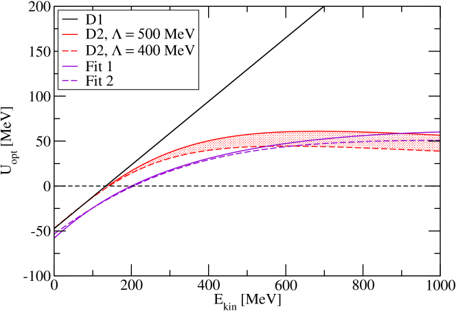
Figure 1: The optical potential $U_{\rm opt}$ as a function of the kinetic energy $E_{\rm kin}=E-m_{\rm nuc}$ of a nucleon in symmetric nuclear matter at saturation density in RMF models with parametrizations D1 and D2 compared to two fits from Dirac phenomenology. See text for details.

The nonlinear derivative couplings are introduced in the RMF model in order to improve the energy dependence of the optical potential $U_{\rm opt}$. The elastic proton scattering on nuclei of different mass number $A$ can be well described in Dirac phenomenology with scalar ($S$) and vector ($V$) potentials, which smoothly vary with $A$ and the energy of the projectile [7, 8]. From these global fits the optical potential in symmetric nuclear matter at saturation density is obtained as a function of the kinetic energy $E_{\rm kin}=E-m_{\rm nuc}$ in the limit $A\to\infty$. There are different definitions of the nonrelativistic optical potential when it is derived from relativistic scalar and vector self-energies. Here we use the form

$$U_{\rm opt}(E)=\frac{E}{m_{\rm nuc}}V-S+\frac{S^{2}-V^{2}}{2m_{\rm nuc}}$$ (47)

with $S=\Sigma_{p}$ and $V=\Sigma_{p}^{0}$ as in references [14, 15, 16, 17, 18]. In conventional RMF models without derivative couplings, the scalar and vector potentials are constant in energy and the optical potential (47) is just a linear function in energy. This is clearly seen in figures 1 and 2 as a full black line for the calculation with the parametrization D1. In contrast, the optical potentials derived from the scalar and vector potentials in Dirac phenomenology from two different fits [7] are much smaller at high energies and exhibit a saturation for $E_{\rm kin}$ approaching $1$ GeV. At low energies, the optical potentials from experiment behave more similar as that of the theoretical model concerning the absolute strength and the energy dependence. In figure 1 (2) the result for the DD-NLD parametrization D2 (D3) is depicted for two values of the cut-off parameter $\Lambda$. Here, a reasonable description of the experimental optical potential is achieved due to the energy dependence of the nucleon self-energies. The difference between parametrizations D2 and D3 is not very significant. The dependence of $U_{\rm opt}$ on $\Lambda$ is stronger for D2. The deflection of the DD-NLD curve for that of the standard RMF model D1 appears at lower kinetic energies for the D3 parametrization as compared to the D2 case. In the DD-NLD model, the optical potential can be calculated easily for other baryon densities and arbitrary neutron-proton asymmetries. Because there are no experimental data available for these general cases, we refrain from presenting the results here. But see reference [14] for the systematics with density in the linear derivative coupling model.

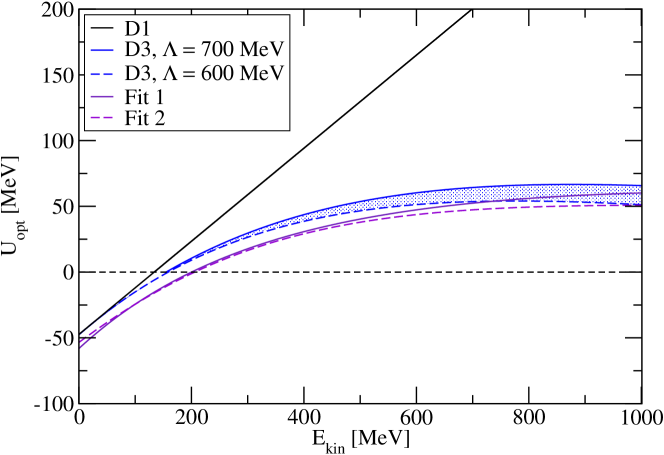
Figure 2: The optical potential $U_{\rm opt}$ as a function of the kinetic energy $E_{\rm kin}$ of a nucleon in symmetric nuclear matter at saturation density in RMF models with parametrizations D1 and D3 compared to two fits from Dirac phenomenology. See text for details.

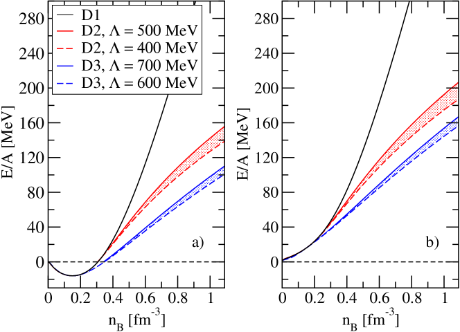
Figure 3: Energy per nucleon $E/A$ as a function of the baryon density $n_{B}$ for symmetric nuclear matter (a) and pure neutron matter (b). Results are given for three different choices of the $D$ function and different values of the cut-off parameter $\Lambda$.

The reduction of the optical potential at high kinetic energies, which originates from the energy dependence of the self-energies, is also reflected in the equation of state. In figure 3 the energy per nucleon $E/A$ (without the rest mass contribution) is depicted as a function of the baryon density $n_{B}$ in symmetric nuclear matter (left panel) and neutron matter (right panel). In both cases, a substantial softening of the EoS is found as compared to the standard RMF calculation with parametrisation D1. The effect is stronger for an exponential energy dependence of the self-energies (D3) than for the case of a Lorentzian dependence (D2). By construction, all EoS are identical at the saturation density $n_{\rm sat}$.

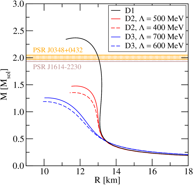
Figure 4: Mass-radius relation of neutron stars for different choices of the $D$ functions and cut-off parameters $\Lambda$ in the DD-NLD model. The two shaded bands refer to astrophysical mass measurements of the pulsars PSR $J1614-2230$ [1] and PSR $J0348+0432$ [2].

The DD-NLD model can be used to predict the properties of neutron stars. Here, the EoS of stellar matter is required. It is obtained by adding the contribution of electrons to the energy density and pressure of the baryons. The conditions of charge neutrality and $\beta$ equilibrium fix the lepton density and proton-neutron asymmetry uniquely. Since the present model calculations treat only homogeneous matter, a suitable EoS for the crust of neutron stars has to be added at low densities. We use the standard Baym-Pethick-Sutherland (BPS) crust EoS [23]. The mass-radius relation of neutron stars is found finally by solving the Tolman-Oppenheimer-Volkoff equations [24, 25]. It is shown for the five models of this work in figure 4 together with the masses of the two most massive pulsars observed so far. The model without an energy dependence (black full line) can explain without any difficulties the large neutron star masses from astrophysical observations [1, 2] because the EoS is rather stiff at high densities. In contrast, for the EoS of neutron star matter in the DD-NLD models that are consistent with the optical potential constraint, a serious reduction of the maximum neutron star mass is seen. These models have even problems to reach typical masses of about $1.4~{}M_{\rm sol}$ of ordinary neutron stars. Deviations from the predictions of the standard model D1 start to appear already at masses below $0.7~{}M_{\rm sol}$. There is also an effect on the neutron star radius, which is found to be smaller in the D2 and in the D3 model. Explicit values for the maximum mass as well as the radius and central density at this extreme conditions are given in table 2. For the DD-NLD models D2 and, in particular, D3 the central densities is a star of maximum mass are considerably higher than those of the standard RMF model without an energy dependence of the couplings.

It is worthwhile to compare our results for the mass-radius relation of neutron stars with those of previous versions of the NLD model. In the approach of reference [18] it was possible to reach a maximum neutron star mass of about $2~{}M_{\rm sol}$ with their choice of parameters. In contrast, the results of reference [19] using different functional forms of the couplings indicate a reduction of the maximum mass below the observed values in line with our calculations. All three versions of the NLD model are adjusted to similar values of the nuclear matter parameters at saturation, such as saturation density, binding energy, compressibility or symmetry energy consistent with experimental constraints. Nevertheless, the predictions for matter properties at supra-saturation densities are rather different due to the various choices in the models to represent the effective in-medium interaction. In our paper, an explicit density dependence of the couplings is considered whereas in [18] nonlinear self-couplings of the meson fields were assumened. In the approach of [19] to nuclear matter neither meson self-couplings nor a density dependence of the couplings were used. A reasonable description of nuclear matter near saturation does not determine the high-density behaviour of the EoS uniquely, in particular due to the additional freedom with the explicit momentum/energy dependence in the NLD approach as compared to standard RMF models. Of course, the maximum mass constraint could be used directly in the determination of the model parameters. But also additional constraints at high densities, e.g. from heavy-ion collisions, might help to reduce the uncertainties in the extrapolation from low to high densities in the future.

Table 2: Maximum mass, corresponding radius and central density of neutrons stars in the DD-NLD models with different parametrizations.

model	$M_{\rm max}$ [$M_{\rm sol}$]	$R(M_{\rm max})$ [km]	$n_{\rm central}(M_{\rm max})$ [fm-3]
D1	2.37	11.57	0.88
D2, $\Lambda=500$ MeV	1.48	11.75	0.95
D2, $\Lambda=400$ MeV	1.36	11.63	0.97
D3, $\Lambda=700$ MeV	1.26	10.13	1.41
D3, $\Lambda=600$ MeV	1.19	9.99	1.46

6 Conclusions

There are several aspects that have to be taken into account in constraining models of dense matter for the application to neutron stars. In phenomenological models, the characteristic saturation properties of nuclear matter and the density dependence of the effective interaction are usually addressed. However, less attention is paid to its energy or momentum dependence.

Introducing non-linear derivative couplings into RMF models, it is possible to generate an energy dependence of the nucleon self-energies such that the optical potential in nuclear matter, which is extracted in Dirac phenomenology from elastic proton-nucleus scattering experiments, can be well described up to energies of $1$ GeV. Considering density-dependent nucleon-meson couplings at the same time, a very flexible model is obtained. Its parameters can be fitted to the usual nuclear matter constraints even for different functional forms of the energy dependent couplings.

In the current version of the DD-NLD model, the energy dependence of the self-energies causes a softening of the EoS at high densities, both for symmetric nuclear matter and pure neutron matter. This effect is independent of the appearance of additional degrees of freedom, such as hyperons or deltas. As a result, it becomes more difficult to obtain very massive neutron stars consistent with the observational constraints. In the present work, the density dependence of the $\omega$ meson coupling was kept fixed in the parametrizations and only a few choices for the energy dependence were tested. Only constraints near the nuclear saturation density were used to determine the model parameters. There remains substantial freedom in the model to be explored in order to find a suitable parametrization that is consistent with the optical potential and maximum neutron mass constraint. Nevertheless, the results of the our study indicate that the optical potential constraint has to be taken seriously into account in the development of realistic phenomenological models for dense matter.

RMF models with self-energies that explicitly depend on the nucleon momentum or energy can be applied to the simulation of heavy-ion collisions using relativistic transport approaches. Here the equation of state can be tested at supra-saturation densities. It is well known that an energy/momentum dependence of the effective in-medium interaction is mandatory for a proper description and analysis of experimental data. Such an approach can help to constrain the parameters of the present model at densities that are not accessible in the description of finite nuclei.

In our work, an explicit energy dependence of the nucleon-meson couplings was favored. It allows to apply the DD-NLD approach to the description of nuclei without major difficulties. Such an additional investigation of the model will permit a better control on the parameters. In particular, the interplay between the choice of the functional form of the energy dependence, the cutoff parameters and the density dependence of the couplings can be studied with its impact for the prediction of maximum neutron star masses. With a larger number of observables as constraints it can be expected that firmer conclusions can be drawn on the compatibility of nuclear matter and finite nuclei descriptions in the DD-NLD model. Work in this direction is in progress.

Appendix A Densities and thermodynamic quantities in the DD-NLD model

The proton and neutron densities (35) in the DD-NLD model are easily calculated through a momentum integration of the relevant integral. For other quantities, however, it is more convenient to introduce an energy integration by substitution because the scalar ($S_{i}$) and vector ($V_{i}$) potentials are explicit functions of the energy $E_{i}$ of the nucleon $i$. With the dispersion relation (43) we obtain

$$p=\sqrt{\left[E_{i}-V_{i}(E_{i})\right]^{2}-\left[m_{i}-S_{i}(E_{i})\right]^{2}}$$ (48)

and the derivative

$$\frac{dp}{dE_{i}}=\frac{1}{p}\left[\left(E_{i}-V_{i}\right)\left(1-\frac{dV_{i}}{dE_{i}}\right)+\left(m_{i}-S_{i}\right)\frac{dS_{i}}{dE_{i}}\right]=\frac{\Pi^{0}_{i}}{p}$$ (49)

with

$$\frac{dV_{i}}{dE_{i}}=\left(\Gamma_{\omega}\omega+\Gamma_{\rho}\tau_{3,i}\rho\right)\frac{dD}{dE_{i}}$$ (50)

and

$$\frac{dS_{i}}{dE_{i}}=\Gamma_{\sigma}\sigma\frac{dD}{dE_{i}}\>.$$ (51)

Introducing the scalar source densities

$$n_{i}^{(sD)} = \kappa_{i}\int_{0}^{p_{Fi}}\frac{d^{3}p}{(2\pi)^{3}}\>\frac{m_{i}^{\ast}}{\Pi_{i}^{0}}D(E_{i})$$

$$= \frac{\kappa_{i}}{2\pi^{2}}\int_{E_{i}^{(\rm min)}}^{E_{i}^{(\rm max)}}dE_{i}\>p(E_{i})\left[m_{i}-S_{i}(E_{i})\right]D(E_{i})$$

and vector source densities

$$n_{i}^{(vD)} = \kappa_{i}\int_{0}^{p_{Fi}}\frac{d^{3}p}{(2\pi)^{3}}\>\frac{E_{i}^{\ast}}{\Pi_{i}^{0}}D(E_{i})$$

$$= \frac{\kappa_{i}}{2\pi^{2}}\int_{E_{i}^{(\rm min)}}^{E_{i}^{(\rm max)}}dE_{i}\>p(E_{i})\left[E-V_{i}(E_{i})\right]D(E_{i})\>,$$

the total source densities

$$n_{\sigma} = n_{p}^{(sD)}+n_{n}^{(sD)}$$ (54)

$$n_{\omega} = n_{p}^{(vD)}+n_{n}^{(vD)}$$ (55)

$$n_{\rho} = n_{p}^{(vD)}-n_{n}^{(vD)}$$ (56)

in the field equations (36), (37), and (38) are found. The lower and upper boundaries of the integrals are determined by solving the equations

$$E_{i}^{(\rm min)}=\left|m_{i}-S_{i}(E_{i}^{(\rm min)})\right|+V_{i}(E_{i}^{(\rm min)})$$ (57)

and

$$E_{i}^{(\rm max)}=\sqrt{p_{Fi}^{2}+\left[m_{i}-S_{i}(E_{i}^{(\rm max)})\right]^{2}}+V_{i}(E_{i}^{(\rm max)})\>,$$ (58)

respectively, with the Fermi momenta $p_{Fi}$ from equation (35). The argument of the coupling functions $n_{v}=n_{p}^{(v)}+n_{n}^{(v)}$ can be obtained from

$$n_{i}^{(v)} = \kappa_{i}\int_{0}^{p_{Fi}}\frac{d^{3}p}{(2\pi)^{3}}\>\frac{E_{i}^{\ast}}{\Pi_{i}^{0}}$$

$$= \frac{\kappa_{i}}{2\pi^{2}}\int_{E_{i}^{(\rm min)}}^{E_{i}^{(\rm max)}}dE_{i}\>p(E_{i})\left[E_{i}-V_{i}(E_{i})\right]\>.$$

The energy density assumes the form

$$\varepsilon = \sum_{i=p,n}\kappa_{i}\int_{0}^{p_{Fi}}\frac{d^{3}p}{(2\pi)^{3}}\>E_{i}-\langle\mathcal{L}\rangle$$

$$= \frac{\kappa_{i}}{2\pi^{2}}\int_{E_{i}^{(\rm min)}}^{E_{i}^{(\rm max)}}dE_{i}\>p(E_{i})\Pi_{i}^{0}(E_{i})E_{i}-\langle\mathcal{L}\rangle$$

and the pressure is given by

$$p = \frac{1}{3}\sum_{i=p,n}\kappa_{i}\int_{0}^{p_{Fi}}\frac{d^{3}p}{(2\pi)^{3}}\>\frac{p^{2}}{\Pi_{i}^{0}}+\langle\mathcal{L}\rangle$$

$$= \sum_{i=p,n}\frac{\kappa_{i}}{6\pi^{2}}\int_{E_{i}^{(\rm min)}}^{E_{i}^{(\rm max)}}dE_{i}\>\left[p(E_{i})\right]^{3}+\langle\mathcal{L}\rangle$$

with

$$\langle\mathcal{L}\rangle=\frac{1}{2}\left(\Gamma_{\omega}\omega n_{\omega}+\Gamma_{\rho}\rho n_{\rho}-\Gamma_{\sigma}\sigma n_{\sigma}\right)+\left(\Gamma_{\omega}^{\prime}\omega n_{\omega}+\Gamma_{\rho}^{\prime}\rho n_{\rho}-\Gamma_{\sigma}^{\prime}\sigma n_{\sigma}\right)n_{v}\>.$$ (62)

Using a partial integration and equation (49), the thermodynamic identity

$$\varepsilon+p = \sum_{i=p,n}\frac{\kappa_{i}}{(2\pi)^{3}}\left.\frac{p^{3}}{3}E_{i}\right|_{0}^{p_{Fi}}$$

$$+\sum_{i=p,n}\frac{\kappa_{i}}{(2\pi)^{3}}\left\{-\frac{1}{3}\int_{0}^{p_{Fi}}d^{3}p\>p\frac{dE_{i}}{dp}+\frac{1}{3}\sum_{i=p,n}\kappa_{i}\int_{0}^{p_{Fi}}d^{3}p\>\frac{p^{2}}{\Pi_{i}^{0}}\right\}$$

$$= \sum_{i=p,n}\mu_{i}n_{i}$$

with the chemical potential $\mu_{i}=E_{i}(p_{Fi})$ is easily confirmed.

References

References

- [1] P. Demorest, T. Pennucci, S. Ransom, M. Roberts, J. Hessels, Shapiro Delay Measurement of A Two Solar Mass Neutron Star, Nature 467 (2010) 1081–1083. arXiv:1010.5788, doi:10.1038/nature09466.
- [2] J. Antoniadis, P. C. Freire, N. Wex, T. M. Tauris, R. S. Lynch, et al., A Massive Pulsar in a Compact Relativistic Binary, Science 340 (2013) 6131. arXiv:1304.6875, doi:10.1126/science.1233232.
- [3] D. Lonardoni, A. Lovato, S. Gandolfi, F. Pederiva, The hyperon puzzle: new hints from Quantum Monte Carlo calculationsarXiv:1407.4448.
- [4] M. Fortin, J. Zdunik, P. Haensel, M. Bejger, Neutron stars with hyperon cores: stellar radii and EOS near nuclear densityarXiv:1408.3052.
- [5] A. Drago, A. Lavagno, G. Pagliara, D. Pigato, Early appearance of Δ isobars in neutron stars, Phys.Rev. C90 (6) (2014) 065809. arXiv:1407.2843, doi:10.1103/PhysRevC.90.065809.
- [6] B.-J. Cai, F. J. Fattoyev, B.-A. Li, W. G. Newton, Critical Density and Impact of Resonance Formation in Neutron StarsarXiv:1501.01680.
- [7] S. Hama, B. Clark, E. Cooper, H. Sherif, R. Mercer, Global Dirac optical potentials for elastic proton scattering from heavy nuclei, Phys.Rev. C41 (1990) 2737–2755. doi:10.1103/PhysRevC.41.2737.
- [8] E. Cooper, S. Hama, B. Clark, R. Mercer, Global Dirac phenomenology for proton nucleus elastic scattering, Phys.Rev. C47 (1993) 297–311. doi:10.1103/PhysRevC.47.297.
- [9] J.-M. Zhang, S. Das Gupta, C. Gale, Momentum dependent nuclear mean fields and collective flow in heavy ion collisions, Phys.Rev. C50 (1994) 1617–1625. arXiv:nucl-th/9405006, doi:10.1103/PhysRevC.50.1617.
- [10] M. Dutra, O. Lourenco, J. Sa Martins, A. Delfino, J. Stone, et al., Skyrme Interaction and Nuclear Matter Constraints, Phys.Rev. C85 (2012) 035201. arXiv:1202.3902, doi:10.1103/PhysRevC.85.035201.
- [11] M. Dutra, O. Lourenço, S. Avancini, B. Carlson, A. Delfino, et al., Relativistic Mean-Field Hadronic Models under Nuclear Matter Constraints, Phys.Rev. C90 (5) (2014) 055203. arXiv:1405.3633, doi:10.1103/PhysRevC.90.055203.
- [12] C. Fuchs, The Relativistic Dirac-Brueckner approach to nuclear matter, Lect.Notes Phys. 641 (2004) 119–146. arXiv:nucl-th/0309003.
- [13] J. Zimanyi, S. Moszkowski, Nuclear Equation of state with derivative scalar coupling, Phys.Rev. C42 (1990) 1416–1421. doi:10.1103/PhysRevC.42.1416.
- [14] S. Typel, T. von Chossy, H. Wolter, Relativistic mean field model with generalized derivative nucleon meson couplings, Phys.Rev. C67 (2003) 034002. arXiv:nucl-th/0210090, doi:10.1103/PhysRevC.67.034002.
- [15] S. Typel, Relativistic model for nuclear matter and atomic nuclei with momentum-dependent self-energies, Phys.Rev. C71 (2005) 064301. arXiv:nucl-th/0501056, doi:10.1103/PhysRevC.71.064301.
- [16] T. Gaitanos, M. Kaskulov, U. Mosel, Non-Linear derivative interactions in relativistic hadrodynamics, Nucl.Phys. A828 (2009) 9–28. arXiv:0904.1130, doi:10.1016/j.nuclphysa.2009.06.019.
- [17] T. Gaitanos, M. Kaskulov, Energy Dependent Isospin Asymmetry in Mean-Field Dynamics, Nucl.Phys. A878 (2012) 49–66. arXiv:1109.4837, doi:10.1016/j.nuclphysa.2012.01.013.
- [18] T. Gaitanos, M. M. Kaskulov, Momentum dependent mean-field dynamics of compressed nuclear matter and neutron stars, Nucl.Phys. A899 (2013) 133–169. arXiv:1206.4821, doi:10.1016/j.nuclphysa.2013.01.002.
- [19] Y. Chen, Relativistic mean field model for nuclear matter with non-linear derivative couplings, Eur.Phys.J. A48 (2012) 132. doi:10.1140/epja/i2012-12132-4.
- [20] Y. Chen, Relativistic mean-field model with nonlinear derivative couplings for nuclear matter and nuclei, Phys.Rev. C89 (6) (2014) 064306. doi:10.1103/PhysRevC.89.064306.
- [21] S. Typel, H. Wolter, Relativistic mean field calculations with density dependent meson nucleon coupling, Nucl.Phys. A656 (1999) 331–364. doi:10.1016/S0375-9474(99)00310-3.
- [22] S. Typel, G. Röpke, T. Klähn, D. Blaschke, H. Wolter, Composition and thermodynamics of nuclear matter with light clusters, Phys.Rev. C81 (2010) 015803. arXiv:0908.2344, doi:10.1103/PhysRevC.81.015803.
- [23] G. Baym, C. Pethick, P. Sutherland, The Ground state of matter at high densities: Equation of state and stellar models, Astrophys.J. 170 (1971) 299–317. doi:10.1086/151216.
- [24] J. Oppenheimer, G. Volkoff, On Massive neutron cores, Phys.Rev. 55 (1939) 374–381. doi:10.1103/PhysRev.55.374.
- [25] R. C. Tolman, Static solutions of Einstein’s field equations for spheres of fluid, Phys.Rev. 55 (1939) 364–373. doi:10.1103/PhysRev.55.364.