On $q$-non-extensive statistics with non-Tsallisian entropy

Abstract

We combine an axiomatics of Rényi with the $q$–deformed version of Khinchin axioms to obtain a measure of information (i.e., entropy) which accounts both for systems with embedded self-similarity and non-extensivity. We show that the entropy thus obtained is uniquely solved in terms of a one-parameter family of information measures. The ensuing maximal-entropy distribution is phrased in terms of a special function known as the Lambert W–function. We analyze the corresponding “high” and “low-temperature” asymptotics and reveal a non-trivial structure of the parameter space.

1 Introduction

In his 1948 paper [1] Shannon formulated the theory of data compression. The paper established a fundamental limit to lossless data compression and showed that this limit coincides with the information measure presently known as Shannon’s entropy ${\mathcal{H}}$. In words, it is possible to compress the source, in a lossless manner, with compression rate close to ${\mathcal{H}}$, it is mathematically impossible to do better than ${\mathcal{H}}$. However, many modern communication processes, including signals, images and coding/decoding systems, often operate in complex environments dominated by conditions that do not match the basic tenets of Shannon’s communication theory. For instance, buffer memory (or storage capacity) of a transmitting channel is often finite, coding can have a non–trivial cost function, codes might have variable-length codes, sources and channels may exhibit memory or losses, etc. Information theory offers various generalized (non–Shannonian) measures of information to deal with such cases. Among the most frequently used one can mention, e.g., Havrda–Charvát measure [2], Sharma–Mittal measure [3], Rényi’s measure [4] or Kapur’s measures [5]. Information entropies get even more complex by considering communication systems with quantum channels [6, 7]. There exists even attempts to generalize Shannon’s measure of information in the direction where no use of the concept of probability is needed hence demonstrating that information is more primitive notion than probability [8].

In mid 1950 Jaynes [9] proposed the Maximum Entropy Principle (MaxEnt) as a general inference procedure that, among others, bears a direct relevance to statistical mechanics and thermodynamics. The conceptual frame of Jaynes’s MaxEnt is formed by Shannon’s communication theory with Shannon’s information measure as an inference functional. The central rôle of Shannon’s entropy as a tool for inductive inference (i.e., inference where new information is given in terms of expected values) was further demonstrated in works of Faddeyev [10], Shore and Johnson [11], Wallis [12], Topsøe [13] and others. In Jaynes’s procedure the laws of statistical mechanics can be viewed as inferences based entirely on prior information that is given in the form of expected values of energy, energy and number of particles, energy and volume, energy and angular momentum, etc., thus re-deriving the familiar canonical ensemble, grand-canonical ensemble, pressure ensemble, rotational ensemble, etc., respectively [14]. Remarkable feature of this procedure is that it entirely dispenses with such traditional hypotheses as ergodicity or metric transitivity. Following Jaynes, one should view the MaxEnt distribution (or maximizer) as a distribution that is maximally noncommittal with regard to missing information and that agrees with all what is known about prior information, but expresses maximum uncertainty with respect to all other matters [9]. By identifying the statistical sample space with the set of all (coarse-grained) microstates the corresponding maximizer yields the Shannon entropy that corresponds to the Gibbs entropy of statistical physics.

Surprisingly, despite the aforementioned connection between information theory and physics and despite related advancements in non-Shannonian information theory, tendencies aiming at similar extensions of the Gibbs’s entropy paradigm started to penetrate into statistical physics only in the last two decades. This happened when evidence accumulated showing that there are indeed many situations of practical interest requiring more “exotic” statistics which do not conform with Gibbsian exponential maximizers. Percolation, protein folding, critical phenomena, cosmic rays, turbulence, granular matter or stock market returns might provide examples.

In attacking the problem of generalization of Gibbs’s entropy the information theoretic route to equilibrium statistical physics provides a very useful conceptual guide. The natural strategy that fits this framework would be then to revisit the axiomatic rules governing Shannon’s information measure and potential extensions translate into language of statistical physics. In fact, the usual axiomatics of Khinchin [15] is prone to several “plausible” generalizations. Among those, the additivity of independent mean information is a natural axiom to attack. Along those lines, two fundamentally distinct generalization schemes have been pursued in the literature; one redefining the statistical mean and another generalizing the additivity rule.

The first mentioned generalization was realized by Rényi by employing the most general means still compatible with Kolmogorov axioms of probability theory. These, so called, quasi-linear means were independently studied by Kolmogorov [16] and Nagumo [17]. It was shown that the generalization based on quasi-linear means unambiguously leads to information measures known as Rényi entropies [4, 18]. Although, the status of Rényi entropies (RE’s) in statistical physics is still debated, they nevertheless provide an immensely important analyzing tool in classical statistical systems with a non-standard scaling behavior (e.g., fractals, multifractals, etc.) [19, 20].

On the other hand, the second approach generalizes the additivity prescription but keeps the usual linear mean. Currently popular generalization is the $q$-additivity prescription and related $q$-calculus [21, 22]. The corresponding axiomatics [23] provides the entropy known as Tsallis–Havrda–Charvát’s (THC) entropy. As the classical additivity of independent information is destroyed in this case, a new more exotic physical mechanisms must be sought to comply with THC predictions. Recent theoretical advances in systems with long-range interactions [26], in generalized (and specifically $q$-generalised) central limit theorems [27], in theory of asymptotic scaling [28], etc., indicate that the typical playground for THC entropy should be in cases where two statistically independent systems have non-vanishing long-range/time correlations or where the notion of statistical independence is an ill-defined concept. Examples include, long-range Ising models, gravitational systems, statistical systems with quantum non-locality, etc.

It is clear that an appropriate combination of the above generalizations could provide a new conceptual paradigm suitable for a statistical description of systems possessing both self-similarity and non-locality. Such systems are quite pertinent with examples spanning from the early universe cosmological phase transitions to currently much studied quantum phase transitions (frustrated spin systems, Fermi liquids, etc.). In passing we should mention that there exists a number of works trying to compare both Rényi and THC entropies from both the theoretical and observational point of view (see, e.g, Refs. [29, 30]). Nevertheless, the merger of both entropic paradigms has not been studied yet. It is aim of this paper to pursue this line of reasonings and explore the resulting implications. In order to set a stage for our considerations we review in the following section some axiomatic essentials for both Shannon, Rényi and THC entropies that will be needed in the main body of the paper. In Section 3 we then formulate a new axiomatics which aims at bridging the Rényi and THC entropies. It is found that such axiomatics allows for only one one-parametric family of solutions. Basic properties of the new entropy that we denote as ${\mathcal{D}}_{q}$ are discussed. A simplification that ${\mathcal{D}}_{q}$ undergoes in multifractal systems is particularly emphasized. The corresponding MaxEnt distributions are calculated in Section 4. We utilize both linear and non–linear moment constraints (applied to the energy) to achieve this goal. In both aforementioned cases the distributions are expressible through the Lambert W–function. Since the analytic structure of MaxEnt distributions is too complex we confine our analysis to the corresponding “high” and “low-temperature” asymptotics and discuss the ensuing non-trivial structure of the parameter space. In Section 5 we discuss the concavity and Schur-concavity of ${\mathcal{D}}_{q}$. Section 6 is devoted to conclusions. The paper is substituted with three appendices which clarify some finer mathematical points.

2 Brief review of entropy axiomatics

The information measure, or simply entropy, is supposed to represent the measure or degree of uncertainty or expectation in conveyed information which is going to be removed by the recipient. As a rule in information theory the exact value of entropy depends only on the information source — more specifically, on the statistical nature of the source. Generally speaking, the higher is the information measure the higher is the ignorance about the system (source) and thus more information will be uncovered after the message is received (or an actual measurement is performed). As often happens, this simple scenario is not frequently tenable as various restrictive factors are present in realistic situations; finite buffer capacity, global patterns in messages, topologically non–trivial sample spaces, etc.. One may even entertain various information theoretic implications related with the quantum probability calculus or quantum communication channels. Thus, as we go to somewhat more elaborate and realistic models, the entropy prescriptions get more complicated and realistic!

To see why a new generalization of the entropy is desirable let us briefly dwell into 3 most common entropy protagonist, namely Shannon’s, Rényi’s and THC entropy.

2.1 Shannon’s entropy — Khinchin axioms

The best known and widely used information measure is Shannon’s entropy. For the completeness sake we now briefly recapitulate the Khinchin axiomatics as this will prove important in what follows. It consist of four axioms [15]:

1. For a given integer $n$ and given ${\mathcal{P}}=\{p_{1},p_{2},\ldots,p_{n}\}$ ($p_{k}\geq 0,\sum_{k}^{n}p_{k}=1$), ${\mathcal{H}}({\mathcal{P}})$ is a continuous with respect to all its arguments.

2. For a given integer $n$, ${\mathcal{H}}(p_{1},p_{2},\ldots,p_{n})$ takes its largest value for $p_{k}=1/n$ ($k=1,2,\ldots,n$).

3. For a given $q\in{\mathbb{R}}$; ${\mathcal{H}}(A\cup B)={\mathcal{H}}(A)+{\mathcal{H}}(B|A)$ with ${\mathcal{H}}(B|A)=\sum_{k}p_{k}\ {\mathcal{H}}(B|A=A_{k})$, and distribution ${\mathcal{P}}$ corresponds to the experiment $A$.

4. ${\mathcal{H}}(p_{1},p_{2},\ldots,p_{n},0)={\mathcal{H}}(p_{1},p_{2},\ldots,p_{n})$, i.e., adding an event of probability zero (impossible event) we do not gain any new information.

The corresponding information measure, Shannon’s entropy, then reads (up to the normalization constant

$${\mathcal{H}}({\mathcal{P}})=-\sum_{k=1}^{n}p_{k}\ln p_{k}\,.$$ (1)

In passing we should stress two important points. Firstly, 3rd axiom (known as separability or strong additivity axiom) indicates that Shannon’s entropy of two independent experiments (sources) is additive. Secondly, there is an intimate connection between the Boltzmann–Gibbs entropy and Shannon’s entropy. In fact, thermodynamics can be viewed as a specific application of Shannon’s information theory: the thermodynamic entropy may be interpreted (when rescaled to “bit” units) as the amount of Shannon information needed to define the detailed microscopic state of the system, which remains “uncommunicated” by a description that is solely in terms of thermodynamic state variables.

2.2 Rény’s entropy: entropy of multifractal systems

As already mentioned, RE represents a step further towards more realistic situations encountered in information theory. Among a myriad of information measures, RE’s distinguish themselves by firm operational characterizations. These were established by Arikan [31] for the theory of guessing, by Jelinek [32] for the buffer overflow problem in lossless source coding, by Cambell [33] for the lossless variable–length coding problem with an exponential cost constraint, etc. Recently, an interesting operational characterization of RE was provided by Csiszár [34] in terms of block coding and hypotheses testing. In the latter case the Rényi parameter $q$ was directly related to so–called $\beta$-cutoff rates [34].

Apart from information theory RE’s have proved to be an indispensable tool also in numerous branches of physics. Typical examples are provided by chaotic dynamical systems and multifractal statistical systems (see e.g., [35] and citations therein). Fully developed turbulence, earthquake analysis and generalized dimensions of strange attractors provide examples.

RE of order $q$ ($q>0$) of a discrete distribution ${\mathcal{P}}=\{p_{1},\ldots,p_{n}\}$ are defined as

$${\mathcal{I}}_{q}({\mathcal{P}})=\frac{1}{(1-q)}\ln\left(\sum_{k=1}^{n}(p_{k})^{q}\right)\,.$$ (2)

In his original work, Rényi [4, 18] introduced a one-parameter family of information measures (2) which he based on axiomatic considerations. In the course of time these axioms have been sharpened by Darótzy [36] and others [37]. Most recently it was shown that RE can be uniquely derived from the following set of axioms [35]:

1. For a given integer $n$ and given ${\mathcal{P}}=\{p_{1},p_{2},\ldots,p_{n}\}$ ($p_{k}\geq 0,\sum_{k}^{n}p_{k}=1$), ${\mathcal{I}}({\mathcal{P}})$ is a continuous with respect to all its arguments.

2. For a given integer $n$, ${\mathcal{I}}(p_{1},p_{2},\ldots,p_{n})$ takes its largest value for $p_{k}=1/n$ ($k=1,2,\ldots,n$).

3. For a given $q\in{{\mathbb{R}}}$; ${\mathcal{I}}(A\cup B)={\mathcal{I}}(A)+{\mathcal{I}}(B|A)$ with ${\mathcal{I}}(B|A)=\mbox{{{g}}}^{-1}\left(\sum_{k}\varrho_{k}(q)\mbox{{{g}}}({\mathcal{I}}(B|A=A_{k}))\right)$, and $\varrho_{k}(q)=p_{k}^{q}/\sum_{k}p_{k}^{q}$  (distribution ${\mathcal{P}}$ corresponds to the experiment $A$). Here g is invertible and positive in $[0,\infty)$.

4. ${\mathcal{I}}(p_{1},p_{2},\ldots,p_{n},0)={\mathcal{I}}(p_{1},p_{2},\ldots,p_{n})$.

Former axioms markedly differ from those utilized in [4, 18, 36, 37]. Particularly distinctive is the presence of the escort (or zooming) distribution $\varrho(q)$ in the 3rd axiom. Distribution $\varrho(q)$ was originally introduced by Rényi [4] to define the entropy associated with the joint distribution. Quite independently was $\varrho(q)$ introduced by Beck and Schlögl [39] in the context of non-linear dynamics.

We briefly remind some elementary properties of ${\mathcal{I}}_{q}$: it is symmetric in all arguments, for ${q}\leq 1$ is ${\mathcal{I}}_{q}$ a concave function and ${\mathcal{H}}({\mathcal{P}})\ \leq\ {\mathcal{I}}_{q}({\mathcal{P}})$, while for ${q}\geq 1$ it is neither concave nor convex and ${\mathcal{I}}_{q}({\mathcal{P}})\ \leq\ {\mathcal{H}}({\mathcal{P}})$. On the other hand, RE of any order are Schur-concave functions [38]. In fact, every function $f({\mathcal{P}})$ which is Schur concave can represent a reasonable measure of information, since it is maximized by a uniform probability distribution, while minimum is provided with concentrated distributions ${\mathcal{P}}=\{p_{i}=1,p_{j\neq i}=0\}$. Some further properties can be found, e.g., in Refs. [4, 18, 35].

Note particularly that RE of two independent experiments (sources) is additive. In fact, it was proved in Ref. [4] that RE is the most general information measure compatible with additivity of independent information and Kolmogorov axioms of probability theory.

2.3 THC entropy: entropy of long distance correlated systems

THC entropy was originally introduced in 1967 by Havrda and Charvát in the context of information theory of computerized systems [2] and together with the $\alpha$-norm entropy measure [40] it belongs to class of pseudo-additive entropies. In contrast with Rényi’s or Shannon’s entropy THC entropy does not have (as yet) an operational characterization. Havrda–Charvát structural entropy, though quite well known among information theorists, had remained largely unknown in physics community. It took more than two decades till Tsallis in his pioneering work [41] on generalized (or non-extensive) statistics rediscovered this entropy. Since then THC entropy has been employed in many physical systems. In this connection one may particularly mention, Hamiltonian systems with long-range interactions, granular systems, complex networks, stock market returns, etc.. For recent review see, e.g., Ref. [42].

In the case of a discrete distribution ${\mathcal{P}}=\{p_{1},\ldots,p_{n}\}$ the THC entropy takes the form:

$${\mathcal{S}}_{q}({\mathcal{P}})=\frac{1}{(1-q)}\left[\sum_{k=1}^{n}(p_{k})^{q}-1\right]\,,\;\;\;\;q>0\,.$$ (3)

Various axiomatic treatments of THC entropy were proposed in the literature. For our purpose the most convenient set of axioms is the following [23]:

1. For a given integer $n$ and given ${\mathcal{P}}=\{p_{1},p_{2},\ldots,p_{n}\}$ ($p_{k}\geq 0,\sum_{k}^{n}p_{k}=1$), ${\mathcal{S}}({\mathcal{P}})$ is a continuous with respect to all its arguments.

2. For a given integer $n$, ${\mathcal{S}}(p_{1},p_{2},\ldots,p_{n})$ takes its largest value for $p_{k}=1/n$ ($k=1,2,\ldots,n$).

3. For a given $q\in{\mathbb{R}}$; ${\mathcal{S}}(A\cup B)={\mathcal{S}}(A)+{\mathcal{S}}(B|A)+(1-q){\mathcal{S}}(A){\mathcal{S}}(B|A)$ with
   $\mbox{\hskip 71.13188pt}{\mathcal{S}}(B|A)=\sum_{k}\varrho_{k}(q)\ {\mathcal{S}}(B|A=A_{k})$,
   and $\varrho_{k}(q)=p_{k}^{q}/\sum_{k}p_{k}^{q}$  (distribution ${\mathcal{P}}$ corresponds to the experiment $A$).

4. ${\mathcal{S}}(p_{1},p_{2},\ldots,p_{n},0)={\mathcal{S}}(p_{1},p_{2},\ldots,p_{n})$.

As we said before, one keeps here the linear mean but generalizes the additivity law. In fact, the additivity law in axiom 3 is nothing but the Jackson sum known from the $q$-calculus [43]; there one defines the Jackson basic number $[X]_{\{q\}}$ of quantity $X$ as

$$[X]_{\{q\}}=(q^{X}-1)/(q-1)\ \Rightarrow\ [X+Y]_{\{q\}}=[X]_{\{q\}}+[Y]_{\{q\}}+(q-1)[X]_{\{q\}}[Y]_{\{q\}}\,.$$ (4)

The connection with axiom 3 is then established when $q\rightarrow(2-q)$. Nice feature of the $q$-calculus is that it formalizes many mathematical manipulations. For instance, using the $q$-logarithm

$$\ln_{\{q\}}x\ =\ -\ln_{\{2-q\}}\left(\frac{1}{x}\right)\ =\ \frac{1}{1-q}\ (x^{1-q}-1)\,,$$ (5)

THC entropy can be concisely written as the $q$-deformed Shannon’s entropy, i.e.,

$${\mathcal{S}}_{q}({\mathcal{P}})\ =\ -\sum_{k=1}^{n}p_{k}\ln_{\{2-q\}}p_{k}\ =\ -\sum_{k=1}^{n}p_{k}^{q}\ln_{\{q\}}p_{k}\ =\ \sum_{k=1}^{n}p_{k}\ln_{\{q\}}\left(\frac{1}{p_{k}}\right)\,.$$ (6)

Some elementary properties of ${\mathcal{S}}_{q}$ are positivity, concavity (and Schur concavity) for all values of $q$ and indeed non-extensivity. There hold also inequalities between all three entropies, namely:

$${\mathcal{H}}({\mathcal{P}})\ \leq\ {\mathcal{I}}_{q}({\mathcal{P}})\ \leq\ {\mathcal{S}}_{q}({\mathcal{P}})\,,$$ (7)

for $0<q\leq 1$, and

$${\mathcal{S}}_{q}({\mathcal{P}})\ \leq\ {\mathcal{I}}_{q}({\mathcal{P}})\ \leq\ {\mathcal{H}}({\mathcal{P}})\,,$$ (8)

for $q\ \geq\ 1$. For a monograph that cover this subject in more depth the reader is referred to Ref. [44].

3 J-A axioms and solutions

It would be conceptually desirable to have a unifying axiomatic framework in which both properties of Rényi and THC entropies are both represented. In Ref. [56] one of us proposed the following natural synthesis of the previous two axiomatics:

1. For a given integer $n$ and given ${\mathcal{P}}=\{p_{1},p_{2},\ldots,p_{n}\}$ ($p_{k}\geq 0,\sum_{k}^{n}p_{k}=1$), ${\mathcal{D}}({\mathcal{P}})$ is a continuous with respect to all its arguments.

2. For a given integer $n$, ${\mathcal{D}}(p_{1},p_{2},\ldots,p_{n})$ takes its largest value for $p_{k}=1/n$ ($k=1,2,\ldots,n$).

3. For a given $q\in{\mathbb{R}}$; ${\mathcal{D}}(A\cup B)={\mathcal{D}}(A)+{\mathcal{D}}(B|A)+(1-q){\mathcal{D}}(A){\mathcal{D}}(B|A)$ with
   $\mbox{\hskip 14.22636pt}{\mathcal{D}}(B|A)=f^{-1}\left(\sum_{k}\varrho_{k}(q)\ f\left({\mathcal{D}}(B|A=A_{k})\right)\right)$,
   and $\varrho_{k}(q)=p_{k}^{q}/\sum_{k}p_{k}^{q}$  (distribution ${\mathcal{P}}$ corresponds to the experiment $A$). Function $f$ is invertible and positive in $[0,\infty)$.

4. ${\mathcal{D}}(p_{1},p_{2},\ldots,p_{n},0)={\mathcal{D}}(p_{1},p_{2},\ldots,p_{n})$.

Note particularly that due to the non-linear nature of the non-additivity condition there is no need to select a normalization condition for ${\mathcal{D}}_{q}$. In Ref. [56] it was shown that above axioms allow for only one class of solutions, leading to an entirely new family of physically conceivable entropy functions. For reader’s convenience are the basic steps of the proof sketched in A. In particular, the resulting hybrid entropy has the following form:

$${\mathcal{D}}_{q}(A)\ =\ \frac{1}{1-q}\ \left(e^{-(1-q)^{2}d{\mathcal{I}}_{q}/dq}\sum_{k=1}^{n}(p_{k})^{q}-1\right)\ =\ \ln_{\{q\}}e^{-\langle\ln{\mathcal{P}}\rangle_{q}}\,.$$ (9)

Let us further remark that axiom 4 restricts the possible values of $q$ to $q\geq 0$. This is because ${\mathcal{D}}_{q}$ would otherwise tend to infinity if some of $p_{k}$ would tend to zero. The latter would be counter-intuitive, because without changing the probability distribution we would gain an infinite information. Value $q=0$ must be also ruled out on the basis of axiom 2, because ${\mathcal{D}}_{0}$ would yield an expression not dependent on the probability distribution ${\mathcal{P}}$ but only on the number of outcomes (or events) — i.e., ${\mathcal{D}}_{0}$ would be a system (source) insensitive. In addition, by further analysis in A, supported by the concept of Schur-concavity in Section 5 we show that ${\mathcal{D}}_{q}$ is well-defined only for $q\geq\frac{1}{2}$. In particular, for $q<\frac{1}{2}$ the entropy ${\mathcal{D}}_{q}$ has a local minimum at ${\mathcal{P}}=\{1/n,\dots,1/n\}$ (rather than maximum) and therefore it does not fulfill axiom 2. Some basic properties of the hybrid entropy ${\mathcal{D}}_{q}$ are presented in B.

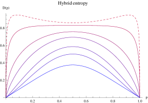
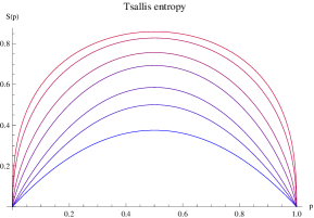
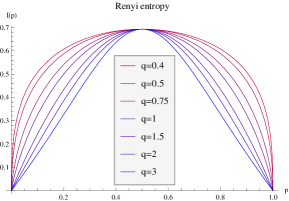
Figure 1: Comparison of entropies for several values of $q$ for two-event systems ($\mathcal{P}=\{p,1-p\}$). The dashed curve represents the hybrid entropy ${\mathcal{D}}_{{}_{0.4}}$ which violates the maximality axiom.

Before studying further implications of the formula (9), there are two immediate consequences which warrant special mention. The first is that, from the condition $d{\mathcal{I}}_{q}/dq\leq 0$ (see Section 2.2) we have

$${\mathcal{D}}_{q}(A)=\left\{\begin{array}[]{ll}\geq\ {\mathcal{S}}_{q}(A)&\mbox{if $q\leq 1$}\\ \leq\ {\mathcal{S}}_{q}(A)&\mbox{if $q\geq 1$}\end{array}\right.\,,$$ (12)

where equality holds, if and only if, $q=1$ or $d{\mathcal{I}}_{q}/dq=0$. These mean that either ${\mathcal{D}}_{q}(A)$ and ${\mathcal{S}}_{q}(A)$ jointly coincide with Shannon’s entropy or that ${\mathcal{P}}$ is uniform or $\{1,0,\ldots,0\}$. Hence, combining this with inequalities between THC, Rényi end Shannon entropy, we obtain

$$0\ \leq\ {\mathcal{H}}({\mathcal{P}})\ \leq\ {\mathcal{I}}_{q}({\mathcal{P}})\ \leq\ {\mathcal{S}}_{q}({\mathcal{P}})\ \leq\ {\mathcal{D}}_{q}({\mathcal{P}})\ \leq\ \ln_{\{q\}}n\,\,\,\,\,\,\,\,\,\mbox{for}\,\,\frac{1}{2}\leq q\leq 1\,,$$

$$0\ \leq\ {\mathcal{D}}_{q}({\mathcal{P}})\ \leq\ {\mathcal{S}}_{q}({\mathcal{P}})\ \leq\ {\mathcal{I}}_{q}({\mathcal{P}})\ \leq\ {\mathcal{H}}({\mathcal{P}})\ \leq\ \ln n\,\,\,\,\,\,\,\,\,\,\,\,\mbox{for}\,\,q\ \geq\ 1\,.$$ (13)

The result (13) implies that by investigating the information measure ${\mathcal{D}}_{q}$ with $q<1$ we receive more information than restricting our investigation just to entropies ${\mathcal{I}}_{q}$ or ${\mathcal{S}}_{q}$. On the other hand, when $q>1$ then both ${\mathcal{I}}_{q}$ and ${\mathcal{S}}_{q}$ are more informative than ${\mathcal{D}}_{q}$. The first set of inequalities is also valid for $q<\frac{1}{2}$, but the last relation to $\ln_{\{q\}}n$ is not true for the hybrid entropy. The practical illustration of the above inequalities can be seen in Fig. 1 for simple distribution ${\mathcal{P}}=\{p,1-p\}$.

In practical cases one usually requires more than one $q$ to gain more complete information about the system. In fact, when entropies ${\mathcal{I}}_{q}$ or ${\mathcal{S}}_{q}$ are used, it is necessary to know them for all $q$ in order to obtain a full information on a given statistical system [35]. For ensuing applications in strange attractors the reader may consult Ref. [46], for reconstruction theorems see, e.g., Refs. [4, 35].

The second comment to be made concerns the fact that when the statistical system in question is a multifractal then relations (97)-(101) assert that

$$(1-q)^{2}\frac{d{\mathcal{I}}_{q}}{dq}\ =\ (a-f(a))\ln\varepsilon\ =\ \ln\left(\sum_{k}^{N(a)}\!p_{k}(\varepsilon)\right)\,,$$ (14)

where summation runs only over support boxes of size $\varepsilon$ with the scaling exponent $a$. Alternatively, we could have started with the first relation in Eq. (89) and use the multifractal canonical relations (see Ref. [35]) in which case the result would have been again (14). So for the coarse-grained multifractal with the mesh size $\varepsilon$ the corresponding entropy ${\mathcal{D}}_{q}$ reads

$${\mathcal{D}}_{q}(A)\ =\ \frac{1}{(1-q)}\left(\frac{\sum_{k=1}^{n}(p_{k}(\varepsilon))^{q}}{\sum_{k}^{N(a)}\!\!p_{k}(\varepsilon)}-1\right)\,.$$ (15)

Now, the passage from multifractals to single–dimensional statistical systems is done by assuming that the $a$-interval is infinitesimally narrow and that PDF is smooth [35, 47]. In such a case Cvitanovic’s condition [47] holds, namely both $a$ and $f(a)$ collapse to $a=f(a)\equiv D$ and $q=f^{\prime}(a)=1$. So, for example, for a statistical system with a smooth PDF and the support space ${\mathbb{R}}^{d}$ the relation (15) implies that the entropy ${\mathcal{D}}_{q}$ coincides with Shannon’s ${\mathcal{H}}$. In this connection it is important to stress that the similarity of (15) with THC entropy is only apparent. In order to have THC entropy one needs to have $N(a)=n$, i.e., the entire probability measure must be accumulated around the unifractal with the scaling exponent $a$. According to the Billingsley (or curdling) theorem [48, 49] this is possible only when $a=f(a)=D$, i.e., only when ${\mathcal{D}}_{q}={\mathcal{H}}$. As a byproduct of Eq. (13) we may notice that for single-dimensional systems with smooth PDF’s ${\mathcal{S}}_{q}$ and ${\mathcal{I}}_{q}$ must approach Shannon’s entropy [35]. We remark that this may help to understand why Shannon’s entropy plays such a predominant rôle in physics of single-dimensional sets.

In what follows, we examine the class of distributions that represent maximizers for ${\mathcal{D}}_{q}(A)$ subject to constraint imposed by the average value of energy.

4 MaxEnt distribution

According to information theory, the MaxEnt principle yields distributions which reflect least bias and maximum uncertainty about information not provided to a recipient (i.e., observer). Important feature of the usual Gibbsian MaxEnt formalism is that the maximal value of entropy is a concave function of the values of the prescribed constraints (moments), and maximizing probabilities are all grater than zero [50]. The first is important for thermodynamical stability and the second for mathematical consistency. In this section we will see that both mentioned features hold true also in the case of the ${\mathcal{D}}_{q}$ entropy.

Let us first address the issue of maximizers for ${\mathcal{D}}_{q}$. To this end we shall seek the conditional extremum of ${\mathcal{D}}_{q}$ subject to the constraints imposed by the averaged value of energy $E$ (or generally any random quantity representing the constant of the motion) in the form

$$\langle E\rangle_{r}\ =\ \sum_{k}\varrho_{k}(r)E_{k}\,.$$ (16)

For the future convenience we initially keep $r$ not necessary coincident with $q$. Taking into account the normalization condition for $p_{i}$ we ought to extremize the functional

$$L_{q,r}({\mathcal{P}})\ =\ {\mathcal{D}}_{q}({\mathcal{P}})-\Omega\ \frac{\sum_{k}(p_{k})^{r}E_{k}}{\sum_{k}(p_{k})^{r}}-\Phi\sum_{k}p_{k}\,,$$ (17)

with $\Omega$ and $\Phi$ being the Lagrange multipliers. Setting the derivatives of $L_{q,r}({\mathcal{P}})$ with respect to $p_{1},p_{2}\ldots,$ etc., to zero, we obtain

$$\frac{\partial L_{q,r}({\mathcal{P}})}{\partial p_{i}}\ = \ e^{(q-1)\sum_{k}\varrho_{k}(q)\ln p_{k}}\left[q(\langle\ln{\mathcal{P}}\rangle_{q}-\ln p_{i})-1\right]\frac{(p_{i})^{q-1}}{\sum_{k}(p_{k})^{q}}$$ (18)

$$- r\Omega\left(E_{i}-\langle E\rangle_{r}\right)\frac{(p_{i})^{r-1}}{\sum_{k}(p_{k})^{r}}-\Phi\ =\ 0\,,\;\;\;\;\;i=1,2,\ldots,n\,.$$

Note that when both $q$ and $r$ approach $1$, (18) reduces to the usual condition for Shannon’s maximizer. This, in turn, ensures that in the $(q,r)\rightarrow(1,1)$ limit the maximizer of (17) is Gibbs’s canonical-ensemble distribution. Let us now concentrate on the two most relevant situations, namely when $r=q$ and $r=1$.

4.1 The $r=q$ case

When we decide to use $r=q$ (i.e., when the non-linear moment constraints are implemented via escort distribution) it follows from (18) that

$$\Phi(p_{i})^{1-q}\sum_{k}(p_{k})^{q}\ =\ e^{(q-1)\langle\ln{\mathcal{P}}\rangle_{q}}\left[q\left(\langle\ln{\mathcal{P}}\rangle_{q}-\ln p_{i}\right)-1\right]-q\Omega(E_{i}-\langle E\rangle_{q})\,.$$ (19)

Multiplying both sides of (19) by $\varrho_{i}(q)$, summing over $i$ and taking the normalization condition $\sum_{k}p_{k}=1$ we obtain

$$\Phi=-e^{(q-1)\langle\ln{\mathcal{P}}\rangle_{q}}\;\;\Rightarrow\;\;\frac{\ln(-\Phi)}{q-1}\ =\ \langle\ln{\mathcal{P}}\rangle_{q}\,\;\;\Rightarrow\;\;{\mathcal{D}}_{q}({\mathcal{P}})|_{\mbox{\footnotesize{max}}}\ =\ \frac{1}{q-1}\ (\Phi+1)\,.$$ (20)

Plugging result (20) back into (19) we obtain after some algebra

$$\sum_{k}(p_{k})^{q}\ =\ (p_{i})^{q-1}\left[q\ln p_{i}+\left(1-\frac{q\ln(-\Phi)}{q-1}-\frac{q\Omega}{\Phi}\ (E_{i}-\langle E\rangle_{q})\right)\right]\,,$$ (21)

which must be true for any index $i$. On the substitution

$${\mathcal{E}}_{i}\ =\ 1-\frac{q\ln(-\Phi)}{q-1}-\frac{q\Omega}{\Phi}\ (E_{i}-\langle E\rangle_{q})\,,$$ (22)

this leads to the equation

$$\kappa(p_{i})^{1-q}\ =\ q\ln p_{i}\ +\ {\mathcal{E}}_{i}\,.$$ (23)

Here we have denoted $\sum_{k}(p_{k})^{q}\equiv\kappa$. Equation (23) has the solution

$$p_{i}\ =\ \left[\frac{q}{\kappa(q-1)}\ W\left(\frac{\kappa(q-1)}{q}\ e^{(q-1){\mathcal{E}}_{i}/q}\right)\right]^{1/(1-q)}\ =\ \exp\left\{\frac{W\left(\frac{\kappa(q-1)}{q}\ e^{(q-1){\mathcal{E}}_{i}/q}\right)}{(q-1)}-{\mathcal{E}}_{i}/q\right\}\,,$$ (24)

with $W(x)$ being the Lambert–W function [51].

A couple of comments are now in order. First, $p_{i}$’s as prescribed by (24) are positive for any value of $q>0$. This is a straightforward consequence of the following two identities [51]:

$$W(x)\ =\ \sum_{n=1}^{\infty}\frac{(-1)^{n-1}n^{n-2}}{(n-1)!}\ x^{n}\,,$$ (25)

$$W(x)\ =\ x\ e^{-W(x)}\,.$$ (26)

Indeed, Eq. (25) ensures that for $x<0$ also $W(x)<0$ and hence $W(x)/x>0$. Thus for $0<q<1$ the positivity of $p_{i}$’s is a simple consequence of the first part of (24). Positivity for $q\geq 1$ follows directly from the relation (26) and the second part of (24).

Second, as $q\rightarrow 1$ the entropy ${\mathcal{D}}_{q}\rightarrow{\mathcal{H}}$ and we expect that $p_{i}$’s defined by (24) should approach the Gibbs canonical-ensemble distribution in this limit. To see that this is indeed the case, let us note that

$$\left.\Phi\right|_{q=1}\ =\ -1\,,\;\;\;\left.{\mathcal{E}}_{i}\right|_{q=1}\ =\ 1+{\mathcal{H}}+\Omega(E_{i}-\langle E\rangle)\,,\;\;\;\mbox{and}\;\;\;\left.\kappa\right|_{q=1}\ =\ 1\,.$$ (27)

Then

$$\left.p_{i}\right|_{q=1}\ =\ e^{1-[1+{\mathcal{H}}+\Omega(E_{i}-\langle E\rangle)]}\ =\ e^{\Omega F-\Omega E_{i}}\ =\ e^{-\Omega E_{i}}/Z\,,$$ (28)

(here $F$ is the Helmholtz free energy) which after identification $\left.\Omega\right|_{q=1}=\beta$ leads to the desired result. Note also that (24) is invariant under uniform translation of the energy spectrum, i.e., the corresponding $p_{i}$ is independent of the choice of the energy origin.

Third, there are situations, when Eq. (23) has no solution, or it gives solution for $p_{i}\not\in[0,1]$. To see this, we may notice that when $q>1$, the left-hand side of (23) is greater than $\kappa$, from which follows that ${\mathcal{E}}_{i}\geq\kappa$ for all $i$’s. For $q<1$ the left-hand side of (23) acquires values from $[0,\kappa]$ which (after using the fact that $q<1<\kappa$) leads again to the condition ${\mathcal{E}}_{i}\geq\kappa$. In both cases are therefore ${\mathcal{E}}_{i}$ positive. Thus, for energies, for which $\Delta_{q}E_{i}=E_{i}-\langle E\rangle_{q}$ is too negative, Eq. (23) has no solution, and the corresponding occupation probability is zero. Contrary to MaxEnt distributions of other commonly used entropies, there exist energy levels here, for which MaxEnt distributions of ${\mathcal{D}}_{q}$ have zero occupation probabilities. This might provide a natural conceptual playground for statistical systems with energy gaps (e.g., disordered systems, carbon nanotubes) or for system with various super-selection rules (e.g., first-quantized relativistic systems).

Finally, there does not seem to by any simple method for a unique determination of $\Phi$ and $\Omega$ from the constraint conditions. In fact, only asymptotic situations for large and vanishingly small $\Omega$ can be successfully resolved (this will be relegated to Sections 4.1.2 and 4.1.3). There exists, however, systems of a practical interest — namely multifractal systems, where we can give to relations (24) a very satisfactory physical interpretation, without resolving $\langle E\rangle_{q}$ in terms of $\Phi$ and $\Omega$.

4.1.1 Multifractal case

In case when a statistical system under investigation fits the multifractal paradigm, we can cast Eq. (23) in the form

$$\varepsilon^{\tau(q)+a_{i}(1-q)}\ \sim\ 1\ +\ q\left[a_{i}-\langle a\rangle_{q}(\varepsilon)\right]\left(1+\frac{\Omega}{\Phi}\right)\ln\varepsilon\,,$$ (29)

where $\tau$ and $a_{i}$ are correlation exponent and Lipshitz–Hölder exponent, respectively. Note that the $q$-mean $\langle a\rangle_{q}(\varepsilon)$ at the coarse-grained scale $\varepsilon$ is proportional to the $q$-mean of log-PDF, namely

$$\langle\ln{\mathcal{P}}\rangle_{q}\ =\ {\sum_{k}\varrho_{k}(q)\ln p_{k}}\ \sim\ {\sum_{k}\varrho_{k}(q)a_{k}\ln\varepsilon}\ =\ \langle a\rangle_{q}(\varepsilon)\ln\varepsilon\,.$$ (30)

So, in particular, $\Phi=-\varepsilon^{(q-1)\langle a\rangle_{q}}$ as can be directly deduced from Eq. (20).

Equation (29) has several important implications. Firstly, we remind the reader that in the long-wave limit (i.e., when $\varepsilon\rightarrow 0$), one can use analogy with ordinary statistical thermodynamics and interpret $\langle a\rangle_{q}$ as the most likely value of “energy” of a system immersed in a heat bath with the effective inverse temperature $\beta=q$ (see, e.g., Ref. [35]). This is a version of the Billingsley (or curdling) theorem [48, 49, 68], which states that the Hausdorff dimension of the set on which the escort probability $\varrho_{k}(q)$ is concentrated is $f(\langle a\rangle_{q})=q\langle a\rangle_{q}-\tau(q)$. In addition, the relative probability of the complement set approaches zero when $\varepsilon\rightarrow 0$. This in turn means that for each $q$ there exists one scaling exponent, namely $a_{i}=\langle a\rangle_{q}$ which dominates, e.g., the partition function $\kappa$, whereas $p_{i}$’s with other Lipshitz–Hölder exponents have only marginal contribution.

Note that the aforesaid indeed mimics the situation occurring in equilibrium statistical physics. There, in the canonical formalism one works with (usually infinite) ensemble of identical systems with all possible energy configurations. But only the configurations with $E_{i}\sim\langle E\rangle_{\beta}$ dominate partition function in the thermodynamic limit. Choice of temperature $T=1/\beta$ then prescribes the contributing energy configurations.

Secondly, for small $\varepsilon$ we have

$$\tau(q)+a_{i}(1-q)\ \sim\ \ln\left\{1\ +\ q\left[a_{i}-\langle a\rangle_{q}(\varepsilon)\right]\left(1+\frac{\Omega}{\Phi}\right)\ln\varepsilon\right\}/\ln\varepsilon\,.$$ (31)

The right-hand side is non-trivial only when

$$\left|q\left(1+\frac{\Omega}{\Phi}\right)\right|\ <\ \frac{1}{\sqrt{-\ln\varepsilon}}\,.$$ (32)

[note that $|a_{i}-\langle a\rangle_{q}|\sim 1/\sqrt{-\ln\varepsilon}$, see Appendix  C]. In such a case Eq. (31) can be recast in the form

$$\tau(q)+a_{i}(1-q)\ \sim\ q\left(1+\frac{\Omega}{\Phi}\right)\left[a_{i}-\langle a\rangle_{q}(\varepsilon)\right]\,,$$ (33)

implying that $\Omega/|\Phi|=(2q-1)/q$. With the help of (32) this means that $q\in[1-1/\sqrt{-\ln\varepsilon},1+1/\sqrt{-\ln\varepsilon}]$. Bearing this in mind we cab write the single-cell probability $p_{i}\sim\varepsilon^{a_{i}}$ as

$$p_{i}\ \sim\ \left[1+(1-q)(a_{i}-\langle a\rangle_{q})\ln\varepsilon\right]^{1/(1-q)}\,.$$ (34)

In multifractals it is more customary to consider the total probability of a phenomenon with a scaling exponent $a_{i}$, i.e., $P_{i}(a)\sim\varepsilon^{-f(a_{i})+a_{i}}$. To this end we can first utilize a simple quadratic expansion

$$f(a_{i})-f(\langle a\rangle_{q})\ =\ q(a_{i}-\langle a\rangle_{q})\ +\ \frac{1}{2}f^{\prime\prime}(\langle a\rangle_{q})(a_{i}-\langle a\rangle_{q})^{2}\ +\ \cdots\ =\ q(a_{i}-\langle a\rangle_{q})\ +\ \frac{1}{2}\frac{(a_{i}-\langle a\rangle_{q})^{2}}{(\Delta a)^{2}\ln\varepsilon}\ +\ \cdots\,.$$ (35)

In the last equality we have employed Eqs. (102)–(103). Note also that the higher-order terms in the expansion (35) are of the order $\mathcal{O}((-\ln\varepsilon)^{-3/2})$. From (29) and (35) we then get

$$P_{i}^{(1-q)}(a)\ \propto\ 1+\ q\left[a_{i}-\langle a\rangle_{q}\right]\left(1+\frac{\Omega}{\Phi}\right)\ln\varepsilon-(1-q)q\left[a_{i}-\langle a\rangle_{q}\right]\ln\varepsilon-(1-q)\frac{1}{2}\frac{(a_{i}-\langle a\rangle_{q})^{2}}{(\Delta a)^{2}}\,.$$ (36)

Since for values $a_{i}$ close to $\langle a\rangle_{q}$ the distribution $P_{i}$ must acquire (due to curdling theorem) a non-trivial value in the limit $\varepsilon\rightarrow 0$, the logarithmic divergences in (36) must cancel each other, yielding the simple condition $\Omega\ =\ q|\Phi|$ . With this we can finally write

$$P_{i}\ \propto\ \left[1\ -\ (1-q)\frac{(a_{i}-\langle a\rangle_{q})^{2}}{2(\Delta a)^{2}}\right]^{1/(1-q)}\,.$$ (37)

This distribution is encountered in a number of multifractal systems. A paradigmatic example can be found in a statistical description of the intermittent evolution of fully-developed turbulence. In such a case $P_{i}(a)$ describes the distribution of singularity exponents of the velocity gradient [61]. In addition, the parameter $q$ satisfies the scaling relation

$$1/(1-q)\ =\ 1/a_{-}\ -\ 1/a_{+}\,,$$ (38)

where $a_{\pm}$ are defined by $f(a_{\pm})=0$. Such a scaling is a manifestation of the mixing property. In Ref. [61] it was further shown that the $q$ variance $(\Delta a)^{2}$ can be related to the phenomenologically important intermittency exponent $\mu$.

4.1.2 “High-temperature” expansion

Let us now make an important remark concerning the asymptotic behavior of $p_{i}$ in regard to $\Omega$. If we assume that the Lagrange multiplier $\Omega\ll 1$ then from (26) the following expansion holds

$$W\!\left(-\frac{\kappa(q-1)}{\Phi q}\ \exp\left(\frac{q-1}{q}\right)\ \exp\left(-(q-1)\frac{\Omega}{\Phi}\Delta_{q}E_{i}\right)\right)\ \approx\ W\!\left(x\right)\left[1\ -\ (1-q)\Omega^{*}\Delta_{q}E_{i}\right]\,,$$ (39)

with

$$\Delta_{q}E_{i}\ =\ E_{i}-\langle E\rangle_{q}\,,\;\;\;\;\;\Omega^{*}\ =\ -\frac{\Omega}{\Phi(W(x)+1)}\,,\;\;\;\;\;x\ =\ -\frac{\kappa(q-1)}{\Phi q}\exp\left(\frac{q-1}{q}\right)\,.$$ (40)

Hence, if we use the relation (24) we can write

$$p_{i}\ =\ \frac{\left[1\ -\ (1-q)\Omega^{*}\Delta_{q}E_{i}\right]^{1/(1-q)}}{\sum_{k}\left[1\ -\ (1-q)\Omega^{*}\Delta_{q}E_{k}\ \ \right]^{1/(q-1)}}\ =\ Z^{-1}\left[1\ -\ (1-q)\Omega^{*}\Delta_{q}E_{i}\right]^{1/(1-q)}\;,$$ (41)

with

$$Z=\sum_{k}\left[1\ -\ (1-q)\Omega^{*}\Delta_{q}E_{k}\ \right]^{1/(1-q)}=\left[\frac{q}{\kappa(q-1)}W(x)\right]^{1/(q-1)}\,.$$ (42)

The distribution (41) agrees with the so called 3rd version of thermostatics introduced by Tsallis et al. [52]. It might by also formally identified with the maximizer for Rényi’s entropy [58]. Clearly, $\Omega^{*}$ is not a Lagrange multiplier, but $\Omega^{*}$ passes to $\beta$ at $q\rightarrow 1$ (in fact, $\Phi\rightarrow-1$, $\Omega\rightarrow\beta$ and $W(x)\rightarrow 0$ at $q\rightarrow 1$). Note also that when $\Omega=0$ (i.e., no energy constraint) then $p_{i}=1/n$ which reconfirms the fact that ${\mathcal{D}}_{q}$ attains its largest value for the uniform distribution.

4.1.3 “Low-temperature” expansion

From the physical standpoint it is the asymptotic behavior at $\Omega\gg 1$ (or more precisely at $\Omega|(q-1)/\Phi|\gg 1$), i.e., “low-temperature” expansion, that is most intriguing. This is because the branching properties of the Lambert–W function at negative argument values make the structure of ${\mathcal{P}}$ rather non-trivial. We thus split our task into four distinct cases:

$$a_{1})\;\;(q-1)>0\;\;\;\; \;\;\;\;\Delta_{q}E<0\,,$$ and

$$a_{2})\;\;(q-1)>0\;\;\;\; \;\;\;\;\Delta_{q}E\geq 0\,,$$ and

$$b_{1})\;\;(q-1)<0\;\;\;\; \;\;\;\;\Delta_{q}E<0\,,$$ and

$$b_{2})\;\;(q-1)<0\;\;\;\; \;\;\;\;\Delta_{q}E\geq 0\,.$$ and

Cases $a_{1})$ and $a_{2})$ are much simpler to start with as the argument of $W$ is positive. $W$ is then a real and single valued function which belongs to the principal branch of $W_{0}$, see Fig.2.

Figure 2: Two real branches of the Lambert–W function. Solid line: $W_{0}(x)\equiv W(x)$ defined for $-1/e\leq x<+\infty$ (so far considered). Dashed line: $W_{-1}(x)$ defined for $-1/e\leq x<0$. The two branches meet at point $(-1/e,-1)$.

When $\Delta_{q}E<0$ then $a_{1})$ implies the asymptotic expansion

$$W\left(z\right)\ \approx\ z\;\;\;\;\Rightarrow\;\;\;\;p_{i}\ =\ \left(\frac{1}{|\Phi|}\right)^{1/(1-q)}\!e^{-1/q}\exp\left(-\frac{\Omega}{|\Phi|}\Delta_{q}E_{i}\right)\ \equiv\ Z_{1}^{-1}\exp\left(-\frac{\Omega}{|\Phi|}\Delta_{q}E_{i}\right)\,,$$ (43)

with

$$Z_{1}\ =\ \left(\frac{1}{|\Phi|}\right)^{1/(q-1)}\!e^{1/q}\,.$$ (44)

Note that in this case $p_{i}$ is of a Boltzmann type ($\langle E\rangle_{q}$ can be canceled against the same term in $Z_{1}$).

On the other hand, $a_{2})$ situation implies the asymptotic expansion [51]

$$W(z)\ \approx\ \ln(z)-\ln(\ln(z))\;\;\;\Rightarrow\;\;\;p_{i}\ =\ Z_{2}^{-1}\left[1-(1-q)\Omega^{*}\Delta_{q}E_{i}\right]^{1/(1-q)}\,,$$ (45)

with

$$Z_{2}\ =\ \left[\frac{q}{\kappa(q-1)}\ln\!\left(\frac{\kappa(q-1)}{|\Phi|q}\exp\left(\frac{q-1}{q}\right)\right)\right]^{1/(q-1)}\;\;;\;\;\Omega^{*}\ =\ \frac{\Omega}{|\Phi|}\left[\ln\!\left(\frac{\kappa(q-1)}{|\Phi|q}\exp\left(\frac{q-1}{q}\right)\right)\right]^{-1}\,.$$ (46)

Although the distribution (45) formally agrees with Tsallis et al. distribution it cannot be identified with it as $\Omega^{*}$ does not tend to $\beta$ in $q\rightarrow 1$ limit. In fact, the limit $q\rightarrow 1$ is prohibited in this case as it violates the “low-temperature” condition $\Omega|(q-1)/\Phi|\gg 1$. Note particularly that our MaxEnt distribution represents in the “low-temperature” regime a heavy tailed distribution with Boltzmannian outset. When $\Omega$ and $q>1$ are fixed one may find $\kappa$ and $\Phi$ from the normalization condition

$$Z_{1}^{-1}\!\!\sum_{k;\Delta_{q}E_{k}<0}\exp\left(-\frac{\Omega}{|\Phi|}\Delta_{q}E_{k}\right)\ +\ Z_{2}^{-1}\!\!\sum_{k;\Delta_{q}E_{k}\geq 0}\left[1-(1-q)\Omega^{*}\Delta_{q}E_{k}\right]^{1/(1-q)}\ =\ 1\,,$$ (47)

and sewing condition at $\Delta_{q}E=0$. However, because the “low-temperature” approximation does not allow to probe regions with small $\Delta_{q}E$ one must numerically optimize the sewing by interpolating the forbidden parts of $\Delta_{q}E$ axis. Example of such a numerical optimization is presented in Fig. 3

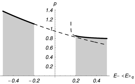
Figure 3: A plot of the “low–temperature” MaxEnt distribution (43)–(45). The parameters of the plot are chosen in the following way: $\kappa=0.01$, $\Phi=-0.68$, $q=30$ and $\Omega=0.5$. The distribution is normalized to $1$ on the interval ${\Delta}_{q}E\in[-0.5,0.5]$.

Cases $b_{1})$ and $b_{2})$ are technically more involved, because $q<1$ causes that the argument of $W(\cdots)$ is negative. In case $b_{1})$ we obtain for low temperatures that

$$\frac{\kappa(q-1)}{q}\exp\left(-(q-1)\frac{\Omega}{\Phi}\Delta_{q}E_{i}\right)\ \rightarrow\ -\infty\,.$$ (48)

Nevertheless, the complex Lambert–W function has a branch cut in the interval $\left[-\infty,-{1}/{e}\right]$, so the real-valued Lambert–W function is defined only for $x>-{1}/{e}$ and Eq. (26) has no real solution. This situation corresponds previous discussions about existence of solution of Eq. (23).

In case $b_{2})$ there exist two solutions of Eq. (26), i.e. $W_{0}(z)$ and $W_{-1}(z)$ (see Fig. 2). In case of the principal branch $W_{0}(z)$, the Lambert W–function can be approximated as $W(z)\approx z$, and the solution corresponds to the case $a_{1})$. In case of the principal branch $W_{-1}(z)$, the asymptotic expansion for $z\rightarrow 0^{-}$ is

$$W_{-1}(z)\ \!\approx\ \!\ln(-z)-\ln(-\ln(-z))$$ (49)

so the resulting probability is similar to the case $a_{2})$, only with

$$\Omega^{*}\ =\ \frac{\Omega}{|\Phi|}\left[\ln\left(\frac{\kappa(1-q)}{|\Phi|q}\exp\left(\frac{q-1}{q}\right)\right)\right]^{-1}\,.$$ (50)

We should stress that for all cases it is necessary to check the validity of the asymptotic expansion and its applicability to the MaxEnt distribution. In some cases can the expansion violate the condition $p_{i}\leq 1$ and then it is not possible to use such approximations.

4.2 The $r=1$ case

When $r=1$ is chosen (i.e., when the constraints are implemented via the usual linear averaging) then Eq.(18) implies

$$\Phi\ =\ e^{(q-1){\langle\ln{\mathcal{P}}\rangle_{q}}}\left[q\left({\langle\ln{\mathcal{P}}\rangle_{q}}-\ln p_{i}\right)-1\right]\,\frac{(p_{i})^{q-1}}{\sum_{k}(p_{k})^{q}}\ -\ \Omega(E_{i}-\langle E\rangle)\,.$$ (51)

Multiplying by $p_{i}$ and summing over $i$ we obtain the constraint

$$\Phi\ =\ -e^{(q-1)\langle\ln{\mathcal{P}}\rangle_{q}}\,\,\Rightarrow\,\,\frac{\ln(-\Phi)}{q-1}\ =\ \langle\ln{\mathcal{P}}\rangle_{q}\,.$$ (52)

Upon insertion of (52) into (51) we get a transcendental equation for $p_{i}$, which reads

$$\kappa p_{i}^{1-q}\ =\ \frac{\Phi}{\Phi+\Omega(E_{i}-\langle E\rangle)}\left[q\ln p_{i}-\frac{q\ln(-\Phi)}{q-1}+1\right]\,.$$ (53)

The solution can be again written in terms of the Lambert W–function, namely

$$p_{i}\ = \ \left[\frac{q\Phi}{(q-1)\kappa(\Phi+\Omega\Delta E_{i})}\;\;W\!\left(-\frac{\kappa(q-1)}{{\Phi}q}\ \exp\left(\frac{q-1}{q}\right)\ \left(1+\frac{\Omega}{\Phi}\Delta E_{i}\right)\right)\right]^{1/(1-q)}$$ (54)

$$= \ \frac{1}{(-\Phi)^{1/(1-q)}e^{1/q}}\ \exp\left\{\frac{1}{(q-1)}\ W\!\left(-\frac{\kappa(q-1)}{{\Phi}q}\ \exp\left(\frac{q-1}{q}\right)\ \left(1+\frac{\Omega}{\Phi}\Delta E_{i}\right)\right)\right\}\,.$$

Relations (25) nad (26) again ensure that all $p_{i}$’s are positive. In addition, it is easy to check that in the limit case $q\rightarrow 1$, the formula (54) approaches the classical Gibbsian maximizer. Indeed, if we utilize the identities:

$$\kappa|_{q=1}\ =\ 1,\;\Phi|_{q=1}\ =\ -1,\;\left[(-\Phi)^{1/(1-q)}\right]|_{q=1}\ =\ e^{-{\mathcal{H}}},\;\;\mbox{and}\;\;\Omega|_{q=1}\ =\ \beta\,,$$ (55)

then

$$p_{i}|_{q=1}\ =\ e^{-{\mathcal{H}}\ +\ \beta(\langle E\rangle-E_{i})}\ =\ e^{\beta F-\beta E_{i}}\ =\ e^{-\beta E_{i}}/Z\,.$$ (56)

Similarly as Eq.(28) also the relation (55) represents an important consistency check of our procedure.

4.2.1 Multifractal case

By following the same strategy as in the case $r=q$, we plug the multifractal scaling relations for $p_{i}\sim\varepsilon^{a_{i}}$ to Eq. (52) and use the fact that the role of $E_{i}$ is taken over by $-a_{i}\ln\varepsilon$. After a short calculation we arrive at

$$\varepsilon^{\tau(q)+a_{i}(1-q)}\left[1-\frac{\Omega}{\Phi}\left(a_{i}-\langle a\rangle_{1}\right)\ln\varepsilon\right]\ \sim\ 1\ +\ q\left(a_{i}-\langle a\rangle_{q}\right)\ln\varepsilon\,,$$ (57)

which in the small-$\varepsilon$ limit yields

$$\tau(q)+a_{i}(1-q)\ +\ \ln\left[1-\frac{\Omega}{\Phi}\left(a_{i}-\langle a\rangle_{1}\right)\ln\varepsilon\right]/\ln\varepsilon\ \sim\ \ln\left[1+q\left(a_{i}-\langle a\rangle_{q}\right)\ln\varepsilon\right]/\ln\varepsilon\ \sim\ 0\,.$$ (58)

The last relation follows from the fact that for $q\geq 1/2$ (cf. A) the expression goes to zero in the small $\varepsilon$ limit. Note that Eq. (58) implies a nontrivial behavior only for

$${\Omega}/{|\Phi|}\ <\ {1}/{\sqrt{-\ln\varepsilon}}\,.$$ (59)

This then gives that

$$\tau(q)+a_{i}(1-q)\ \sim\ \frac{\Omega}{\Phi}(a_{i}-\langle a\rangle_{1})\,,$$ (60)

and hence $\Omega/|\Phi|=q-1$. Latter shows in particular that $q\in[1,1+1/\sqrt{-\ln\varepsilon}]$. Rather than dealing with the single-cell probability $p_{i}$ we can again address the (more relevant) total probability $P_{i}(a)\sim\varepsilon^{a_{i}-f(a_{i})}$. By using the fact that (cf. Eq. (60))

$$\tau(q)+[a_{i}-f(a_{i})](1-q)+\frac{\Omega}{|\Phi|}(a_{i}-\langle a\rangle_{1})+f(a_{i})(1-q)\ \sim\ 0,$$ (61)

and the expansion

$$f(a_{i})-f(\langle a\rangle_{1})\ =\ (a_{i}-\langle a\rangle_{1})\ +\ \frac{1}{2}f^{\prime\prime}(\langle a\rangle_{1})\left(a_{i}-\langle a\rangle_{1}\right)^{2}\ +\ \cdots\ =\ \left(a_{i}-\langle a\rangle_{1}\right)\ +\ \frac{1}{2}\frac{(a_{i}-\langle a\rangle_{1})^{2}}{(\Delta a)^{2}\ln\varepsilon}\ +\ \cdots\,.$$ (62)

[in the second equality we have used again the curdling theorem (see C)], we obtain

$$P_{i}(a)\ \sim\ \left[1\ -\ \frac{(1-q)}{2}\frac{\left(a_{i}-\langle a\rangle_{1}\right)^{2}}{(\Delta a)^{2}}\right]^{1/(1-q)}.$$ (63)

This prescription naturally appears in the context of multiplicative cascades with the coarse-grained scaling $\varepsilon=2^{-k}$ ($k\geqq 1$). Again, the natural application would be in a fully-developed turbulence. The proximity of $q$ to one makes the previous distribution suitable for discussions concerning the dynamics on the measure theoretic support, i.e., a set whose Hausdorff–Besicovich dimension is $a(1)=f(a(1))$. In particular, it can be shown [59] that the measure theoretic support describe the set on which the probability is concentrated.

4.2.2 “High-temperature” expansion

Similarly as in the $r=q$ case we can find the “high-temperature” expansion by assuming that $\Omega\ll 1$. In such a case we have

$$\frac{\Phi}{(\Phi+\Omega\Delta E_{i})}\;W\!\left(-\frac{\kappa(q-1)}{{\Phi}q}\ \exp\left(\frac{q-1}{q}\right)\ \left(1+\frac{\Omega}{\Phi}\Delta E_{i}\right)\right)\ \approx\ W(x)\left[1-(1-q)\Omega^{*}\Delta E_{i}\right]\,.$$ (64)

Here

$$\Omega^{*}=-\frac{q}{q-1}\frac{\Omega W(x)}{\Phi(W(x)+1)}\,,\;\;\;\;\;x\ =\ -\frac{\kappa(q-1)}{\Phi q}\exp\left(\frac{q-1}{q}\right)\,.$$ (65)

Through (54) this implies that

$$p_{i}\ =\ Z^{-1}\left[1\ -\ (1-q)\Omega^{*}\Delta E_{i}\right]^{1/(1-q)}\;,$$ (66)

with

$$Z=\sum_{k}\left[1\ -\ (1-q)\Omega^{*}\Delta E_{k}\ \right]^{1/(1-q)}=\left[\frac{q}{\kappa(q-1)}W(x)\right]^{1/(q-1)}\,.$$ (67)

Relation (66) coincides with the Tsallis-type distribution that is historically known as Bashkirov’s 1st version of thermostatistics [58].

Note in passing that by using the identity $\lim_{q\rightarrow 1}W(x)/(q-1)=1$, we obtain that the factor $\Omega^{*}$ approaches the inverse temperature $\beta$ in the limit $q\rightarrow 1$ as it should.

4.2.3 “Low-temperature” expansion

We now wish to consider the “low-temperature” expansion — i.e., $\Omega\gg 1$. Similarly as in the $r=q$ case, we divide the situation into four sub-cases:

$$a_{1})\;\;(q-1)>0\;\;\;\; \;\;\;\;\Delta E<0\,,$$ and

$$a_{2})\;\;(q-1)>0\;\;\;\; \;\;\;\;\Delta E\geq 0\,,$$ and

$$b_{1})\;\;(q-1)<0\;\;\;\; \;\;\;\;\Delta E<0\,,$$ and

$$b_{2})\;\;(q-1)<0\;\;\;\; \;\;\;\;\Delta E\geq 0\,.$$ and

Unlike case $r=q$, the sub-cases group into two qualitatively distinct classes:

1. cases $a_{2})$ and $b_{1})$ lead to the asymptotic expansion $W(z)\propto\ln(z)-\ln(\ln(z))$, because $-\frac{k(q-1)\Delta E_{i}}{\Phi^{2}q}>0$.

2. cases $a_{1})$ and $b_{2})$ lead to the situation, when the Lambert W–function is not defined, which corresponds to the fact that Eq. (53) has no solution.

So in particular, we see that in cases when our hybrid entropy cannot be consistently used over the whole temperature range. It can be at best used as an effective entropy in higher-temperature regimes. This might be particularly pertinent in the high-energy particle phenomenology where the host of phase transitions is happening under conditions that are far from thermal equilibrium (e.g., chiral phase transition in QCD and ensuing quark-gluon plasma formation). In the first case, i.e., when the asymptotic expansion exists, the probability distribution can be written in the form

$$p_{i}\ =\ \left\{\frac{\frac{\kappa(q-1)}{q}\left(1+\Omega\Delta E_{i}\right)}{\ln\left[-\frac{\kappa(q-1)}{q\phi}\exp\left(\frac{q-1}{q}\right)\right]+\ln\left[1+\Omega\Delta E_{i}\right]}\right\}^{{1}/(q-1)}\,.$$ (68)

Contrary to $r=q$, the resulting distribution has functionally different form from both the Boltzmann distribution and Tsallis distribution, even in the generalized form, i.e. with the self-referential temperature. For large temperatures, the second term in the denominator is negligible and the distribution becomes similar to power-like behavior. We shall again note that it is necessary to check consistency of asymptotic expansions.

5 Concavity and Schur-concavity of ${\mathcal{D}}_{q}$

In this section we discuss the concavity properties of ${\mathcal{D}}_{q}$. When referring to concavity issue of entropies, one has to distinguish between two types of concavity. In thermodynamics, the important issue is to show whether or not the thermodynamical entropy is a concave function of extensive variables. This means to show that ${\mathcal{D}}_{q}|_{\mbox{\footnotesize{max}}}$ is a concave function under the constraints as in the case of Gibbsian MaxEnt. Note that in contrast to the information-theoretic entropy ${\mathcal{D}}_{q}$, ${\mathcal{D}}_{q}|_{\mbox{\footnotesize{max}}}$ is the system entropy, i.e., it depends on the actual system state variables.

In the information theory, the significance of concavity lies in the fact that it automatically ensures the validity of the maximality axiom. In case of ${\mathcal{D}}_{q}$, it suffices to explore the concavity issue only for $e^{-\langle\ln\mathcal{P}\rangle_{q}}$ because $\ln_{\{q\}}$ is concave and non-decreasing function for all $q>0$,

$$\frac{\partial^{2}}{\partial p_{i}^{2}}\left(e^{-\langle\ln\mathcal{P}\rangle_{q}}\right)\ =\ e^{-\langle\ln\mathcal{P}\rangle_{q}}\left[\left(\frac{\partial\langle\ln\mathcal{P}\rangle_{q}}{\partial p_{i}}\right)^{2}-\frac{\partial^{2}\langle\ln\mathcal{P}\rangle_{q}}{\partial p_{i}^{2}}\right].$$ (69)

It can be shown that the bracket is always negative for $q\in[\frac{1}{2},1]$. Contrary, for $q>1$ we have that $\frac{\partial^{2}\langle\ln\mathcal{P}\rangle_{q}}{\partial p_{i}^{2}}\left|{}_{p_{i}\rightarrow 0}\right.=-\infty$, while the first term remains bounded and therefore the function cannot be concave for all $p_{i}$’s.

However, concavity is only a sufficient condition that ensures the maximality axiom. As known, e.g., from the case of Rényi entropy, there are examples of non-concave entropies which still have well defined global maximum at $\mathcal{P}=\{1/n,\ldots,1/n\}$. In fact, there exist weaker concepts that ensure validity of the maximality axiom. Among these the most prominently is the notion of Schur-concavity [70]. The overview of applications of Schur-concavity can be found in Refs. [71, 72]. This concept is based on the idea of majorization. We say that a probability distribution $\mathcal{P}=\{p_{1},\dots,p_{n}\}$ is majorized by distribution $\mathcal{Q}=\{q_{1},\dots,q_{n}\}$ if for ordered probability vectors $p_{(1)}\geq p_{(2)}\geq\dots$, resp. $q_{(1)}\geq q_{(2)}\geq\dots$ hold $\sum_{k=1}^{j}p_{(k)}\leq\sum_{k=1}^{j}q_{(k)}$, where $j=1,\dots,{n-1}$ (for $j=n$ is the inequality fulfilled automatically from normalization). We denote $\mathcal{P}\prec\mathcal{Q}$. We say that the function $F$ is Schur-concave if for $\mathcal{P}\prec\mathcal{Q}$ is $F(\mathcal{P})\geq F(\mathcal{Q})$. The Schur-concavity automatically preserves the maximality axiom, because the uniform distribution is majorized by every other distribution. Shi et al. have shown [73] that special subclass of functions called Gini means (defined e.g. in Ref. [74]) that can be expressed in the form

$$G(q;x,y)=\exp\left(\frac{x^{q}\ln x+y^{q}\ln y}{x^{q}+y^{q}}\right)\,,$$ (70)

is for $(x,y)\in\mathds{R}^{2}_{+}$ Schur-convex function of $(x,y)$ when $2q\geq 1$ (this is a consequence of [73, Theorem 1] for $r=s$). It is then easy to shown that $\mathcal{D}_{q}$ is Schur-concave function for $q\geq\frac{1}{2}$. As a consequence, for $q\geq\frac{1}{2}$, $\mathcal{D}_{q}$ fulfills the maximality axiom. Moreover, Ref. [73] discussed the case $q\in(0,\frac{1}{2}$ and concluded that one cannot say anything about Schur-convexity or Schur-concavity of ${\mathcal{D}}_{q}$ on this interval. For illustration, in Fig. 1 we compare three types of entropies, i.e., $\mathcal{D}_{q}$, $\mathcal{S}_{q}$ and $\mathcal{I}_{q}$ for various values of $q$ on distribution ${\mathcal{P}}=\{p,1-p\}$, and we observe that $\mathcal{D}_{0.4}$ is neither Schur-convex nor Schur-concave, which is caused by the fact that maximum is not in $\mathcal{P}=\left\{1/n,\dots,1/n\right\}$.

6 Conclusions and outlooks

We have presented a plausible generalization of the information entropy concept. Our approach is based on an axiomatic merger of two currently widely used information measures: Rényi’s and Tsallis–Havrda–Charvát’s. Such a merger is natural from the mathematical point of view as both above measures have an axiomatic underpinning with a very similar axiomatics. From the physics viewpoint the above merger is interesting because it combines two entropies with analogous MaxEnt distributions but with very different scope of applicability in physics.

We have shown that the maximizers for ${\mathcal{D}}_{q}$ subject to constant averaged energy are represented in terms of the Lambert W–function. The Lambert W–function is a special function that appears in numerous exactly solvable statistical systems. Tonks gas [53], Richards growth model and Lotka–Volterra models [54] may serve as examples. The Lambert W–function was recently also used in quantum statistics [55] and statistics of weak long-range repulsive potentials [53]. This usage nicely bolsters our suggestion that a typical playground for ${\mathcal{D}}_{q}$ could be in statistical systems with both self-similarity and non-locality. In addition, as a byproduct, we have obtained during our analysis some new mathematical properties of the Lambert W–function.

Due to complicated analytical structure of the MaxEnt distribution we have resorted in our discussion to the “low” and “high temperature” asymptotic regimes. We have shown that under certain parameter conditions these have the heavy tailed behavior that is identical with Tsallisian maximizers. The fact that this is true only asymptotically might be at first sight a bit surprising, as there exists perception that both THC and Rényi’s entropies have the same maximizer and hence the merger entropy should again posses the same MaxEnt distribution. This anticipation is clearly erroneous. Indeed, both Rényi entropy and THC maximizers have the same functional form but their respective“temperature” parameters $\beta^{*}$ are entirely different functions of $q$, and in the case of THC entropy $\beta^{*}$ is even self-referential (i.e., it depends on the distribution itself) [58].

In summary, we have shown that there exists a well defined sense in which one can combine Rényi and THC entropic paradigms. We have found the associated one-parametric class of entropy measures, namely (9) and the ensuing MaxEnt distributions (24). It can be rightly objected that apart from the axiomatic side more is needed to consider ${\mathcal{D}}_{q}$ as a legitimate object of statistical physics. In this connection one should, however, stress that the presented entropy has a number of desirable attributes; like THC entropy it is a one-parametric class of entropies satisfying the non-extensive $q$-additivity, it goes over into ${\mathcal{H}}({\mathcal{P}})$ in the $q\rightarrow 1$ limit, it complies with thermodynamic stability, continuity, symmetry, expansivity, decisivity, Schur concavity, etc. On that basis it appears that both ${\mathcal{D}}_{q}$ and THC entropies have an equal right to serve as a generalization of statistical thermodynamics.

7 Acknowledgements

We acknowledge very helpful discussions with P.T. Landsberg, P. Haramoës and H. Lavička which have helped us to understand better the ideas discussed in this paper. The work was supported by the Grant Agency of the CTU in Prague, grant No. SGS13/217/OHK4/3T/14 and the GAČR, grant No. GA14-07983S.

Appendix A Derivation of ${\mathcal{D}}_{q}$ from J-A axioms

In this appendix we show the basic steps in the derivation of functional form of hybrid entropy ${\mathcal{D}}_{q}$.

Let us first denote ${\mathcal{D}}(1/n,1/n,\ldots,1/n)={\mathcal{L}}(n)$. Axioms $2$ and $5$ then imply that ${\mathcal{L}}(n)={\mathcal{D}}(1/n,\ldots,1/n,0)\ \leq\ {\mathcal{D}}(1/{n+1},\ldots,1/{n+1})={\mathcal{L}}(n+1)$. Consequently ${\mathcal{L}}$ is a non-decreasing function of $n$. To determine the explicit form of ${\mathcal{L}}(n)$ we will assume that $A^{(1)},\ldots,A^{(m)}$ are independent experiments each with $r$ equally probable outcomes, so

$${\mathcal{D}}(A^{(k)})={\mathcal{D}}(1/r,\ldots,1/r)={\mathcal{L}}(r)\,,\;\;\;\;(1\leq k\leq m)\,.$$ (71)

Repeated application of axiom $3$ then leads to

$${\mathcal{D}}(A^{(1)}\cup A^{(2)}\cup\ldots\cup A^{(m)})={\mathcal{L}}(r^{m}) = \sum_{k=1}^{m}{}^{m}C_{k}\ (1-q)^{k-1}{\mathcal{D}}^{k}(A^{(k)})$$ (72)

$$= \frac{1}{(1-q)}\left[\left(1+(1-q){\mathcal{L}}(r)\right)^{m}-1\right]\,,$$

where ${}^{m}C_{k}$ is the binomial coefficient. By assuming that (72) can be extended from $m\in{\mathbb{N}}_{+}$ to ${\mathbb{R}}_{+}$ we can take partial derivative of both sides of (72) with respect to $m$ and by setting $m=1$ we obtain the differential equation

$$\frac{(1-q)\ d{\mathcal{L}}}{(1+(1-q)\ {\mathcal{L}})\left[\ln\left(1+(1-q)\ {\mathcal{L}}\right)\right]}\ =\ \frac{dr}{r\ln r}\,.$$ (73)

The general solution of (73) has the form

$${\mathcal{L}}(r)\ \equiv\ {\mathcal{L}}_{q}(r)\ =\ \frac{1}{1-q}\left(r^{c(q)}-1\right)\,.$$ (74)

The integration constant $c(q)$ will be determined shortly. Right now we just note that because at $q=1$ Eq.(72) boils down to ${\mathcal{L}}(r^{m})=m{\mathcal{L}}(r)$ we must have $c(1)=0$. In addition, the monotonicity of ${\mathcal{L}}(r)$ ensures that $c(q)/(1-q)\geq 0$. To proceed further let us consider the experiment with outcomes $A=(A_{1},A_{2},\ldots,A_{n})$ and the distribution ${\mathcal{P}}=\{p_{1},p_{2},\ldots,p_{n}\}$. Assume moreover that $p_{k}\,(1\leq k\leq n)$ are rational numbers, i.e.,

$$p_{k}=\frac{g_{k}}{g}\,,\;\;\;\;\sum_{k=1}^{n}g_{k}=g\,,\;\;\;\;g_{k}\in\mathbb{Z}^{+}\,.$$ (75)

Let have, in addition, an experiment $B=(B_{1},B_{2},\ldots,B_{g})$ with associated distribution ${\mathcal{Q}}=\{q_{1},q_{2},\ldots,q_{g}\}$. We split $(B_{1},B_{2},\ldots,B_{g})$ into $n$ groups containing $g_{1},g_{2},\ldots,g_{n}$ outcomes respectively. Consider now a particular situation in which whenever event $A_{i}$ in $A$ happens then in $B$ all $g_{k}$ events of $k$-th group occur with the equal probability $1/g_{k}$ and all the other events in $B$ have probability zero. Hence

$${\mathcal{D}}(B|A=A_{k})={\mathcal{D}}(1/g_{k},\ldots,1/g_{k})={\mathcal{L}}_{q}(g_{k})\,,$$ (76)

and so axiom $3$ implies that

$${\mathcal{D}}(B|A)=f^{-1}\left(\sum_{k=1}^{n}\varrho_{k}(q)f({\mathcal{L}}_{q}(g_{k}))\right)\,.$$ (77)

On the other hand, in the stated system the entropy ${\mathcal{D}}(A\cup B)$ can be easily evaluated. Realizing that the joint probability distribution corresponding to $A\cup B$ is

$${\mathcal{R}}\ =\ \left\{r_{kl}\ =\ p_{k}q_{l|k}\right\}\ =\ \{\underbrace{\frac{p_{1}}{g_{1}},\ldots,\frac{p_{1}}{g_{1}},}_{g_{1}\times}\underbrace{\frac{p_{2}}{g_{2}},\ldots,\frac{p_{2}}{g_{2}},}_{g_{2}\times}\ldots,\underbrace{\frac{p_{n}}{g_{n}},\ldots,\frac{p_{n}}{g_{n}}}_{g_{n}\times}\}\ =\ \left\{1/g,\ldots,1/g\right\}\,,$$ (78)

we obtain that ${\mathcal{D}}(A\cup B)={\mathcal{L}}_{q}(g)$. Applying axiom 3 together with (74) we get

$${\mathcal{D}}(A)\left(1+(1-q)f^{-1}\left(\sum_{k}\varrho_{k}(q)f({\mathcal{L}}_{q}(p_{k})[1+(1-q){\mathcal{L}}_{q}(g)]+{\mathcal{L}}_{q}(g))\right)\right)$$

$$\mbox{\hskip 56.9055pt}=\ {\mathcal{L}}_{q}(g)-f^{-1}\left(\sum_{k}\varrho_{k}(q)f({\mathcal{L}}_{q}(p_{k})[1+(1-q){\mathcal{L}}_{q}(g)]+{\mathcal{L}}_{q}(g))\right)\,.$$ (79)

Define $f_{(a,y)}(x)=f(-ax+y)\,\Rightarrow\ f^{-1}(x)-y=-af^{-1}_{(a,y)}(x)\;$ then

$${\mathcal{D}}(A)=\frac{f^{-1}_{(a,{\mathcal{L}}(g))}\left(\sum_{k}\varrho_{k}(q)f_{(a,{\mathcal{L}}_{q}(g))}(-{\mathcal{L}}(p_{k}))\right)}{1-(1-q)f^{-1}_{(a,{\mathcal{L}}(g))}\left(\sum_{k}\varrho_{k}(q)f_{(a,{\mathcal{L}}_{q}(g))}(-{\mathcal{L}}(p_{k}))\right)},$$ (80)

with $a=[1+(1-q){\mathcal{L}}_{q}(g)]$.

To proceed further, let us formally put $p_{k}=1/r$. Eq. (74) then indicates that it is ${\mathcal{L}}_{q}(1/p_{k})$ and not $-{\mathcal{L}}_{q}(p_{k})$ which represents the elementary information of order $q$ affiliated with $p_{k}$ (cf. with Eq. (5)). It is thus convenient to reformulate (80) directly in terms of ${\mathcal{L}}_{q}(1/p_{k})$. This can be done via relation

$${\mathcal{L}}_{q}(p_{k})=-\frac{{\mathcal{L}}_{q}(1/p_{k})}{1+(1-q){\mathcal{L}}_{q}(1/p_{k})}\,.$$ (81)

If we now write

$${\textsl{g}}(x)=f_{(a,{\mathcal{L}}(g))}\left(\frac{x}{1+(1-q)x}\right)\,,$$ (82)

we easily obtain from (80) that

$${\mathcal{D}}(A)={\textsl{g}}^{-1}\left(\sum_{k}\varrho_{k}(q){\textsl{g}}({\mathcal{L}}_{q}\left(1/p_{k}\right))\right)\,.$$ (83)

Moreover, if we set in the second part of axiom 3, $B=A$ then ${\mathcal{D}}(A)$ is given as

$${\mathcal{D}}(A)=f^{-1}\left(\sum_{k}\varrho_{k}(q)f({\mathcal{L}}_{q}\left(1/p_{k}\right))\right)\,.$$ (84)

Using the fact that two quasi-linear means with the same ${\mathcal{P}}$ are identical iff their respective Kolmogorov–Nagumo functions are linearly related [4], we may write

$${\textsl{g}}(x)=f\left(\frac{-x+y}{1+(1-q)x}\right)=\theta_{q}(y)f(x)\ +\ \vartheta_{q}(y)\,.$$ (85)

Here $y={\mathcal{L}}_{q}(g)$. In order to solve (85) we define $\varphi(x)=f(x)-f(0)$. With this notation Eq. (85) turns into

$$\varphi\left(\frac{-x+y}{1+(1-q)x}\right)=\theta_{q}(y)\varphi(x)\ +\ \varphi(y)\,,\;\;\;\;\;\varphi(0)=0\,.$$ (86)

By setting $x=y$ we obtain that $\theta_{q}(y)=-1$, and hence

$$\varphi(x+y+(1-q)xy)\ =\ \varphi(x)+\varphi(y)\,.$$ (87)

According to axiom 1 we may now extend (87) to real valued $x$ and $y$. Eq.(87) is Pixeder’s functional equation which can be solved by the standard method of iterations [45]. In [69] we have shown that (87) has only one non-trivial class of solutions, namely

$$\varphi(x)=\frac{1}{\alpha}\ln\left[1+(1-q)x\right]\,.$$ (88)

$\alpha$ is here a free parameter. By inserting this solution back to (84) we obtain

$${\mathcal{D}}_{q}(A) = \frac{1}{1-q}\ \left(e^{-c(q)\sum_{k}\varrho_{k}(q)\ln p_{k}}-1\right)=\frac{1}{1-q}\left(\prod_{k}(p_{k})^{-c(q)\varrho_{k}(q)}-1\right)\,.$$ (89)

Note that the constant $\alpha$ got canceled. We have also denoted the explicit order of the entropy ${\mathcal{D}}$ with the subscript $q$. It remains to determine $c(q)$. Utilizing the conditional entropy constructed from (89) and using axiom $3$, we obtain $c(q)=1-q$. In result we can recast (89) into more expedient form. By utilizing

$$\langle\ln{\mathcal{P}}\rangle_{q}\ =\ (1-q)\frac{\mathrm{d}{\mathcal{I}}_{q}({\mathcal{P}})}{\mathrm{d}{q}}-{\mathcal{I}}_{q}({\mathcal{P}})\,.$$ (90)

the following results holds

$${\mathcal{D}}_{q}(A)\ =\ \frac{1}{1-q}\ \left(e^{-(1-q)^{2}d{\mathcal{I}}_{q}/dq}\sum_{k=1}^{n}(p_{k})^{q}-1\right)\,.$$ (91)

Restrictions on $q$ from the maximality axiom

In the foregoing proof we have used the axiom 2 to show that $\mathcal{L}(n+1)\geq\mathcal{L}(n)$, which in turn yielded $\mathcal{L}(n)=\ln_{\{q\}}(n)$, cf. Eq. (74). We have not, however, checked whether the global maximum is really at $\mathcal{P}=\{1/n,\dots,1/n\}$. In situation when the entropy is a (Schur-)concave function on the probability space, we obtain the maximality directly. This is the case, e.g., for both Rényi and THC entropy. Unfortunately, a (Schur-)concavity of $\mathcal{D}_{q}$ is ensured only for certain values of $q$ (as discussed in Section 5). Here we illustrate the fact that $\mathcal{D}_{q}$ can have maxima in other points than $\mathcal{P}=\{1/n,\dots,1/n\}$. To this end we note from (9) that because $\ln_{\{q\}}(x)$ is a monotonous function for $x>0$ and since $e^{-x}$ is a positive monotonous function on $\mathds{R}$, we can consider only $\langle\ln\mathcal{P}\rangle_{q}$. For simplicity’s sake, we present the analysis only for probability distribution of two events, i.e., $\mathcal{P}=\{p,1-p\}$. The analysis for more outcomes is similar, the only difference is that one has to employ the Lagrange multipliers to account for the fact that the probability vector is confined on a simplex.

Stationary points of $\langle\ln\mathcal{P}\rangle_{q}$ are solutions of the equation

$$\mbox{}\frac{\mathrm{d}}{\mathrm{d}p}\left(\frac{p^{q}\ln p+(1-p)^{q}\ln(1-p)}{p^{q}+(1-p)^{q}}\right) = \frac{1}{Z(q)^{2}}\left[p^{2q-1}-(1-p)^{2q-1}+p^{q-1}(1-p)^{q}-p^{q}(1-p)^{q-1}\right.$$ (92)

$$\left.-qp^{q}(1-p)^{q-1}\ln\left(\frac{1-p}{p}\right)+qp^{q-1}(1-p)^{q}\ln\left(\frac{p}{1-p}\right)\right]\ =\ 0\,.$$

The factor ${Z(q)^{2}}={[p^{q}+(1-p)^{q}]^{2}}$ is positive and can be thus omitted from the further analysis. After the substitution $y={p}/{(1-p)}$ the previous equation reduces to

$$y^{2q-1}-y^{q}(1-q\ln y)+y^{q-1}(1+q\ln y)-1\ =\ 0\,,$$ (93)

or alternatively to

$$\Psi_{q}(y)\ \equiv\ q\ln y-\frac{1-y^{q-1}+y^{q}-y^{2q-1}}{y^{q}+y^{q-1}}\ =\ 0\,.$$ (94)

The interesting property of $\Psi_{q}(y)$ is that $\Psi_{q}\left(\frac{1}{y}\right)=-\Psi_{q}(y)$ and $\Psi_{1}(y)=\ln y$.

The equation $\Psi_{q}(y)=0$ has for $q\geq\frac{1}{2}$ only one solution, which is $y=1$, or equivalently $x=\frac{1}{2}$. However, for $q<\frac{1}{2}$, there occur two more solutions, related by the reciprocity relation. As a consequence, from the nature of $\langle\ln\mathcal{P}\rangle_{q}$ one can deduce, that the point $x=\frac{1}{2}$ corresponds to the local minimum, while other two points represent global maxima. Eventually, the second axiom is violated for $q<\frac{1}{2}$ and $\mathcal{D}_{q}$ is therefore well defined only for $q\geq\frac{1}{2}$.

Appendix B Basic properties of ${\mathcal{D}}_{q}$ entropy

In this appendix, we list some basic properties of the hybrid entropy ${\mathcal{D}}_{q}$.

Let us start with features that ${\mathcal{D}}_{q}$ shares with both Rényi’s and THC entropies. These are

(a) ${\mathcal{D}}_{q}({\mathcal{P}}=\{1,0,\ldots,0\})=0$

(b) ${\mathcal{D}}_{q}({\mathcal{P}})\geq 0$

(c) ${\mathcal{D}}_{1}={\mathcal{I}}_{1}={\mathcal{S}}_{1}={\mathcal{H}}$

(d) ${\mathcal{D}}_{q}$ involves a single free parameter - $q$

(e) ${\mathcal{D}}_{q}$ is symmetric, i.e., ${\mathcal{D}}_{q}(p_{1},\ldots,p_{n})={\mathcal{D}}_{q}(p_{k(1)},\ldots,p_{k(n)})$

(f) ${\mathcal{D}}_{q}$ is bounded

On the other hand, among features inherited from Rényi’s entropy we can find that

(g) ${\mathcal{D}}_{q}(A)=f^{-1}\left(\sum_{k}\varrho_{k}(q)f({\mathcal{D}}_{q}(A_{k}))\right)$

(h) For single-dimensional statistical systems with continuous PDF ${\mathcal{D}}_{q}(A)$ reduces to ${\mathcal{H}}$

(i) ${\mathcal{D}}_{q}$ is a strictly decreasing function of $q$, i.e., $d{\mathcal{D}}_{q}/dq\leq 0$, for any $q>0$

Result (i) follows from the fact that ${\mathcal{D}}_{q}$ is a monotonically decreasing function of $A_{q}\equiv\sum_{k}\varrho_{k}(q)\ln p_{k}$ (see Eq.(89)) and that $A_{q}$ is a monotonically increasing function of $q$, indeed

$$\frac{dA_{q}}{dq}\ =\ \langle(\ln({\mathcal{P}}))^{2}\rangle_{q}-\langle\ln({\mathcal{P}})\rangle_{q}^{2}\ \geq\ 0\,.$$ (95)

Here $\langle\ldots\rangle_{q}$ is defined with respect to the distribution $\varrho_{k}(q)$. The last relation in (95) is Jensen’s inequality. Note that $d{\mathcal{D}}_{q}/dq=0$ happens only for the degenerate case ${\mathcal{P}}=\{1,\ldots,0\}$ (and ensuing permutations).
here Finally, properties taken over from THC entropy include

(j) $\max_{{\mathcal{P}}}{\mathcal{D}}_{q}({\mathcal{P}})={\mathcal{D}}_{q}({\mathcal{P}}=\{1/n,\ldots,1/n\})=\ln_{\{q\}}n$         (for $q>1/2$)

(k) ${\mathcal{D}}_{q}$ is $q$ non–extensive, i.e., ${\mathcal{D}}(A\cup B)={\mathcal{D}}(A)+{\mathcal{D}}(B|A)+(1-q){\mathcal{D}}(A){\mathcal{D}}(B|A)$

Appendix C Some essentials of the multifractal formalism

We present here some essentials of the fractal and multiftactal calculus that are employed in the main body of the text.

Fractals are sets with a generally non–integer dimension exhibiting property of self–similarity. The key characteristic of fractals is a fractal dimension which is defined as follows: Consider a set $M$ embedded in a $d$–dimensional space. Let us cover the set with a mesh of $d$–dimensional cubes of size $\varepsilon^{d}$ and let $N_{\varepsilon}(M)$ is a number of the cubes needed for the covering. The fractal dimension of $M$ is then defined as [48, 59]

$$D=-\lim_{\varepsilon\rightarrow 0}\frac{\ln N_{\varepsilon}(M)}{\ln\varepsilon}\,.$$ (96)

The dimension defined in (96) is also known as box-counting dimension. In most cases of interest the latter coincides with the Hausdorff–Besicovich dimension used by Mandelbrot [48].

Multifractals, on the other hand, are related to the study of a distribution of physical or other quantities on a generic support (be it or not fractal) and thus provide a move from the geometry of sets as such to geometric properties of distributions. Let us suppose that over some support (usually a subset of a metric space) is distributed a probability of a certain phenomenon. If we pave the support with a grid of spacing $\varepsilon$ and denote the integrated probability in the $i$th box as $p_{i}$, then the scaling exponent $a_{i}$ is defined [48, 59]

$$p_{i}(\varepsilon)\sim{\varepsilon}^{a_{i}}\,.$$ (97)

The exponent $a_{i}$ is called singularity or Lipshitz–Hölder exponent. Counting boxes $N(a)$ where $p_{i}$ has $a_{i}\in(a,a+da)$, the singularity spectrum $f(a)$ is defined as [48, 59]

$$N(a)\sim{\varepsilon}^{-f(a)}\,.$$ (98)

Thus a multifractal is the ensemble of intertwined (uni)fractals each with its own fractal dimension $f(a_{i})$. It is further convenient to define a “partition function” [48]

$$Z(q)=\sum_{i}(p_{i}(\varepsilon))^{q}=\int da^{\prime}\rho(a^{\prime}){\varepsilon}^{-f(a^{\prime})}{\varepsilon}^{qa^{\prime}}\,,$$ (99)

($\rho(a)$ is a proportionality function having its origin in relations (97) and (98)). In the small $\varepsilon$ limit the method of steepest descent yields the scaling

$$Z(q)\sim{\varepsilon}^{\tau(q)}\,,$$ (100)

with

$$\tau(q)=\min_{a}[qa-f(a)],\,\,f^{\prime}(a)=q\,\,\,\mbox{and}\,\,\,\tau^{\prime}(q)=a(q)\,.$$ (101)

These are precisely Legendre transform relations. Scaling exponent $\tau$ is often called the correlation exponent. Legendre transform (101) ensures that pairs $f(a),a$ and $\tau(q),q$, are conjugates comprising the same mathematical content.

It is an important consequence of (99) that the relative fluctuations of the Lipshitz–Hölder exponent $a$ around its mean value $\langle a\rangle_{q}$ are very small in the $\varepsilon\rightarrow 0$ limit. This is because

$$\partial^{2}(\ln Z(q))\partial q^{2}\ =\ \left[\langle a^{2}\rangle_{q}\ -\ \langle a\rangle_{q}^{2}\right](\ln\varepsilon)^{2}\ \equiv\ (\Delta a)^{2}(\ln\varepsilon)^{2}\,,$$ (102)

$$\partial^{2}(\tau\ln\varepsilon)\partial q^{2}\ =\ \left({da}/{dq}\right)\ln\varepsilon\ =\ \left[{1}/{f^{\prime\prime}(a)}\right]\ln\varepsilon\,.$$ (103)

Since both left-hand sides in (102) and (103) are identical, we can infer from a finiteness of $f^{\prime\prime}(a)$ that the standard deviation of $a$ is of order $1/\sqrt{-\ln\varepsilon}$. So for small $\varepsilon$ the $a$-fluctuations become negligible and almost all $a$ equal to $\langle q\rangle_{q}$. Note also that because the variance $(\Delta a)^{2}>0$ and $\ln\varepsilon<0$, we have that $f^{\prime\prime}(a)<0$, i.e., the $f(a)$ function is concave.

The fact that for a given $q$ the total probability of a phenomenon with a scaling exponent $a_{i}$ is concentrated around the value $a_{i}\sim\langle a\rangle_{q}$ is known as the curdling theorem [48] (or Billingsley theorem [49]) and it represents a particular example of the so-called measure concentration phenomenon [60].

Multifractal formalism has direct applications in the turbulent flow of fluids [61], percolation [62], diffusion–limited aggregation (DLA) systems [63], DNA sequences [64], finance [65, 67], string theory [66], etc.. In chaotic dynamical systems all ${\mathcal{I}}_{q}$ are necessary to describe uniquely, e.g., strange attractors [46]. More generally, one may argue [35] that when the outcome space is discrete then all ${\mathcal{I}}_{q}$ (or ${\mathcal{S}}_{q}$) with $q\in[1,\infty)$ but are needed to reconstruct the underlying distribution, while when the outcome space is $d$-dimensional subset of ${\mathbb{R}}^{d}$ then all ${\mathcal{I}}_{q}$ (or ${\mathcal{S}}_{q}$), $q\in(0,\infty)$, are required to pinpoint uniquely the underlying PDF. The latter can be viewed as the information–theoretic variants of Hausforff’s moment problem of mathematical statistics.

The connection of Rényi entropies with multifractals is established via relation (99). Note particularly that when $\varepsilon$ is finite then ${\mathcal{I}}_{q}$ plays the rôle of the Helmholtz free energy. Closer analysis of the related implications can be found, e.g., in Refs. [35, 68].

References

- [1] C.E. Shannon A mathematical theory of communication, Bell Syst. Tech. J. 27, (1948), 379; 623.
- [2] J.H. Havrda and F. Charvat, Kybernatika 3 (1967) 30.
- [3] B.D. Sharma and D.P. Mittal, J. Math. Sci. 10 (1975) 28.
- [4] A. Rényi, Selected Papers of Alfred Rényi, Vol.2 (Akadémia Kiado, Budapest, 1976).
- [5] J.N.Kapur, The Mathematics Seminar 4 (1967) 78; Ind. Jour. Pure and App. Maths. 17 (1986) 429.
- [6] M. Müller-Lennert, F. Dupuis, O. Szehr, S. Fehr and M. Tomamichel, J. Math. Phys. 54 (2013) 122203.
- [7] P.J. Coles and M. Piani, Phys. Rev. A 89 (2014) 022112.
- [8] K. Urbanik, Rep. Math. Phys. 4 (1973) 289.
- [9] E.T. Jaynes, Phys. Rev. 106 (1957) 171; 108(1957) 620.
- [10] D.K Faddeyev, Uspekhi Mat. Nauk, 11 (1956) 227 .
- [11] J.E. Shore and R.W. Johnson, IEEE Trans. Inform. Theory 26(1980) 26.
- [12] in, E.T. Jaynes, Probability Theory, The Logic of Science (Cambrideg Un. Press, Cambridge, 2003).
- [13] F. Topsøe, Kybernetika 15 (1979) 8; IEEE Trans. Inform. Theory 48 (2002) 2368.
- [14] E.T. Jaynes, Revs. Modern. Phys. 27 (1955) 189.
- [15] A.I. Khinchin, Mathematical Foundations of Information Theory (Dover Publications, Inc., New York, 1957).
- [16] A. Kolmogorov, Atti della R. Accademia Nazionale dei Lincei 12 (1930) 388.
- [17] M. Nagumo, Japanese Jour. Math. 7 (1930) 71.
- [18] A. Rényi, Probability Theory (North-Holland, Amsterdam, 1970).
- [19] T.C. Halsey, M.H. Jensen, L.P. Kadanoff, I. Procaccia and B.I. Shraiman, Phys. Rev. A 33 (1986) 1141; M.H. Jensen, L.P. Kadanoff, A. Libchaber, I. Procaccia and J. Stavans, Phys. Rev. Lett. 55 (1985) 2798; K. Tomita, H. Hata, T. Horita, H. Mori and T. Morita, Prog. Theor. Phys. 80 (1988) 963; H.G.E. Hentschel and I. Procaccia, Physica D 8 (1983) 435.
- [20] D. Harte, Multifractals, Theory and Applications (Chapman & Hall/CRC London,2001).
- [21] V.G. Drinfeld, Quantum Groups, in: A. Gleason, ed., Proc. Intern. Congr. Math. (Berkeley, 1986) p. 798.
- [22] M. Jimbo, Lett. Math. Phys. 10 (1985) 63.
- [23] S. Abe, Phys. Let. A 271 (2000) 74.
- [24] G. Kaniadakis, Phys. Rev. E 66 (2002) 056125; G. Kaniadakis, M. Lissia and A.M. Scarfone, [cond-mat/0409683].
- [25] J. Naudts, Physica A 340 (2004) 32.
- [26] T. Dauxois, S. Ruffo, E. Arimondo and M. Wilkens, eds. Dynamics and Thermodynamics of Systems with Long range Interactions, Lecture Notes in Physics, vol.602 (Springer, Berlin, 2002).
- [27] H. Suyari, IEEE Trans. Inform. Theory 50 (2004) 1783.
- [28] R. Hanel and S. Thurner, Entropy 15, (2013) 5324.
- [29] J.-F. Bercher, Entropies and entropic criteria, in: Regularization and Bayesian Methods for Inverse Problems in Signal and Image Processing J.-F. Giovannelli and J. Idier eds. (Wiley, New York, 2015), pp 267.
- [30] Christiane F. L. Lima et al, A Comparative Study of Use of Shannon, R nyi and Tsallis Entropy for Attribute Selecting in Network Intrusion Detection, In Proceedings 13th International Conference, Natal, Brazil, August 29-31, 2012.
- [31] E. Arikan, IEEE Trans. Inform. Theory 42(1996) 99.
- [32] F. Jelinek, Probabilistic Information Theory (McGraw-Hill, New York, 1968).
- [33] L.L. Cambell, Inform. Contr., 8 (1965) 423.
- [34] I. Csiszár, IEEE Trans. Inform. Theory 41 (1995) 26.
- [35] P. Jizba and T. Arimitsu, Annals of Phys. (NY) 312 (2004) 17.
- [36] Z. Daróczy, Acta Mathematica Academiae Scientiarium Hungaricae 15 (1964) 203.
- [37] see e.g., S. Guias, Information Theory with Applications. (McGraw-Hill, New York, 1977) .
- [38] Z. Puchała, Ł. Rudnicki and K. Życzkowski, J. Phys. A: Math. Theor. 46 (2013) 272002.
- [39] C. Beck and F. Schlögl, Thermodynamics of Chaotic systems: An Introduction (Cambridge Un. Press., Cambridge, 1997).
- [40] S. Arimito, Inform. Contr. 45 (1980) 136.
- [41] C. Tsallis, J. Stat Phys. 52 (1988) 479; Braz. J. Phys. 29 (1999) 1.
- [42] C. Tsallis, Introduction to Nonextensive Statistical Mechanics; Approaching a Complex World (Springer, New York, 2009).
- [43] F.H. Jackson, Q. J. Pure Appl. Math. 41 (1910) 193; Am. J. Math. 32 (1910) 305; V.G. Drinfeld, Quantum Groups, in: A. Gleason,Bill ed., Proc. Intern. Congr. Math. (Berkeley, 1986), p. 798; M. Jimbo, Lett. Math. Phys. 10 (1985) 63.
- [44] see e.g., S. Abe and Y. Okamoto (Eds.), Nonextensive Statistical Mechanics and Its Applications (Springer-Verlag, New York, 2001) and monographs in http://tsallis.cat.cbpf.br/biblio.htm .
- [45] J. Aczél, Lectures on Functional Equations and their Applications (Academic Press, New York, 1966).
- [46] H.G.E. Hentschel and I. Procaccia, Physica D 8 (1983) 435.
- [47] P. Cvitanovic, Classical and Quantum Chaos, http://www.nbi.dk/ChaosBook .
- [48] B.B. Mandelbrot, Fractal–Form, Chance and Dimension (Freeman, San francisco, 1977).
- [49] P. Billingsley, Ergodic Theory and Information, (Willey, New York, 1965).
- [50] H.B. Callen, Thermodynamics and an introduction to thermostatistics (Wiley, New York, 1985).
- [51] R.M. Corless, G.H. Gonnet, D.E. Hare, D.J. Jeffrey and D.E. Knuth, Adv. Comput. Math. 5 (1996) 329.
- [52] C. Tsallis, R.S. Mendes and A.R. Plastino, Physica A 261 (1998) 534.
- [53] J.-M. Caillol, J. Phys. A: Math. Gen. 36 (2003) 10431.
- [54] K.M. Briggs, W-ology, or, some exactly solvable growth models, unpublished notes; 1998 February 16; Department of Plant Sciences, University of Cambridge, http://www-epidem.plantsci.cam.ac.uk//W-ology.html).
- [55] S.R. Valluri, M. Gil, D.J. Jeffrey, and S. Basu, J. Math. Phys. 50 (2009) 102103.
- [56] P. Jizba and T. Arimitsu, Physica A 340 (2004) 110.
- [57] T.D. Frank and A. Daffertshofer, Physica A 285 (2000) 351.
- [58] A.G. Bashkirov and A.D. Sukhanov, JETP 95 (2002) 440; A.G. Bashkirov, Physica A 340 (2004) 153.
- [59] J. Feder, Fractals (Plenum Press, New York, 1988).
- [60] P. Jizba and T. Arimitsu, Phys. Rev. E 69 (2004) 026128.
- [61] U. Frisch and G. Parisi, in Turbulence and Predictibility in Geophysical Fluid Dynamics and Climate Dynamics (editors M. Ghil, R Benzi and G. Parisi, North–Holland, New York, 1985); T. Arimitsu and N. Arimitsu, Physica A 295 (2001) 177; T. Arimitsu and N. Arimitsu, J. Phys. A: Math. Gen. 33 (2000) L235 [corrigendum: 34 (2001) 673]; T. Arimitsu and N. Arimitsu, Physica A 305 (2002) 218; T. Arimitsu and N. Arimitsu, J. Phys.: Condens. Matter 14 (2002) 2237; T. Arimitsu and N. Arimitsu,“Analysis of Accelerations in Turbulence based on Generalized Statistics” (2002), [cond–mat/0203240].
- [62] A. Aharony, in Time–Dependent Effects in Disordered Materials (editors R. Pynn and T. Riste, Plenum Press, New York, 1987).
- [63] C. Amitrano, A. Coniglio and F. di Liberto, Phys. Rev. Lett. 57 (1986) 1016.
- [64] Zu-Guo Yu, Vo Anh, Ka-Sing Lau, Phys. Rev. E 64 (2001) 031903.
- [65] V.V. Anh, Q.M. Tieng and Y.K. Tse, Intl. Trans. in Op. Res. 7 (2000) 349.
- [66] M. Mineev-Weinstein, P.B. Wiegmann and A. Zabrodin, Phys. Rev. Lett. 84 (2000) 5106.
- [67] P. Jizba and J. Korbel, Physica A 413 (2014) 438.
- [68] P. Jizba, Information theory and generalized statistics, in: H.–T. Elze, ed., Decoherence and Entropy in Complex Systems, Lecture Notes in Physics, Vol. 633 (Springer-Verlag, Berlin 2003), p.362.
- [69] G.H. Hardy, J.E. Littlewood and G. Pólya, Inequalities (Cambridge University Press, Cambridge, 1952).
- [70] W. Shu-hong, Z. Tian-yu, X. Bo-yan Communications in Computer and Information Science 243 (2011) 626.
- [71] A. W. Marshal and I. Olkin, Mathematics and Science and Engineering 143 (1979).
- [72] A. W. Roberts and D. E. Varberg, Pure and Applied Mathematics 57 (1973) 12.
- [73] Huan-Nan Shi, Yong-Ming Jiang and Wei-Dong Jiang, Computers and Mathematics with Applications 57 (2009) 266.
- [74] P. S. Bullen, D. S. Mitrinovi and P. M. Vasi , Means and Their Inequalities (Springer, Netherlands, 1988).