Hardness of Virtual Network Embedding with Replica Selection

Abstract

Efficient embedding virtual clusters in physical network is a challenging problem. In this paper we consider a scenario where physical network has a structure of a balanced tree. This assumption is justified by many real-world implementations of datacenters.

We consider an extension to virtual cluster embedding by introducing replication among data chunks. In many real-world applications, data is stored in distributed and redundant way. This assumption introduces additional hardness in deciding what replica to process.

By reduction from classical NP-complete problem of Boolean Satisfiability, we show limits of optimality of embedding. Our result holds even in trees of edge height bounded by three. Also, we show that limiting replication factor to two replicas per chunk type does not make the problem simpler.

1 Introduction

Server virtualization has revamped the server business over the last years, and has radically changed the way we think about resource allocation: today, almost arbitrary computational resources can be allocated on demand. Moreover, the virtualization trend now started to spill over to the network: batch-processing applications such as MapReduce often generate significant network traffic (namely during the so-called shuffle phase) [18], and in order to avoid interference in the underlying physical network and in order to provide a predictable application performance, it is important to provide performance isolation and bandwidth guarantees for the virtual network connecting the virtual machines. [10]

Prominent example of large-scale framework that is used in datacenters is MapReduce. In such applications often network usage becomes the limiting factor for application performance. Sharing single link among multiple node-node communications requires reserving certain amount of network traffic to avoid slowing the transfer down. In order to model MapReduce execution, bandwidth has to be reserved for transfer of chunks to nodes and for node-node interconnection. Resulting virtual network to be embedded consists of clique and single links incoming to its vertices. Described abstraction is called virtual cluster [3, 16].

Our Contributions.We show that minimizing network footprint is NP-hard in presence of multiple replicas of the same chunk type. Moreover, we show that NP-hard problems already arise in small-diameter networks (as they are widely used today [1]), and even if the number of replicas is bounded by two.

2 Model

To get started, and before introducing our formal model and its constituting parts in detail, we will discuss the practical motivation.

2.1 Background and Practical Motivation

Our model is motivated by batch-processing applications such as MapReduce. Such applications use multiple virtual machines to process data, initially often redundantly stored in a distributed file system implemented by multiple servers. [6] The standard datacenter topologies today are (multi-rooted) fat-tree resp. Clos topologies [1, 8], hierarchical networks recursively made of sub-trees at each level; servers are located at the tree leaves. Given the amount of multiplexing over the mesh of links and the availability of multi-path routing protocol, e.g. ECMP, the redundant links can be considered as a single aggregate link for bandwidth reservations [3, 16].

During execution, batch-processing applications typically cycle through different phases, most prominently, a mapping phase and a reducing phase; between the two phases, a shuffling operation is performed, a phase where the results from the mappers are communicated to the reducers. Since the shuffling phase can constitute a non-negligible part of the overall runtime [4], and since concurrent network transmissions can introduce interference and performance unpredictability [18], it is important to provide explicit minimal bandwidth guarantees [10]. In particular, we model the virtual network connecting the virtual machines as a virtual cluster [3, 10, 16]; however, we extend this model with a notion of data-locality. In particular, we distinguish between the bandwidth needed between assigned chunk and virtual machine ($b_{1}$) and the bandwidth needed between two virtual machines ($b_{2}$); in practice, for applications with a large ’’mapping ratio‘‘ where the mapping phase already reduces the data size significantly, it may hold that $b_{2}\ll b_{1}$.

2.2 Fundamental Parts

Let us now introduce our model more formally. It consists of three fundamental parts: (1) the substrate network (the servers and the connecting physical network), (2) the to be processed input (the data chunks), and (3) the virtual network (the virtual machines and the logical network connecting the machines to each other as well as to the chunks).

The Substrate Network. The substrate network (also known as the host graph) represents the physical resources: a set $S$ of $n_{S}=|S|$ servers interconnected by a network consisting of a set $R$ of routers (or switches) and a set $E$ of (symmetric) links; we will often refer to the elements in $S\cup R$ as the vertices. We will assume that the inter-connecting network forms an (arbitrary, not necessarily balanced or regular) tree, where the servers are located at the tree leaves. Each server $s\in S$ can host zero or one virtual machine. Each link $e\in E$ has a certain bandwidth capacity $\emph{cap}(e)$.

The Input Data. The to be processed data constitutes the input to the batch-processing application. The data is stored in a distributed manner; this spatial distribution is given and not subject to optimization. The input data consists of $\tau$ different chunk types $\{c_{1},\ldots,c_{\tau}\}$, where each chunk type $c_{i}$ can have $r_{i}\geq 1$ instances (or replicas) $\{c_{i}^{(1)},\ldots,c_{i}^{(r_{i})}\}$, stored at different servers. It is sufficient to process one replica, and we will sometimes refer to this replica as the active (or selected) replica.

The input data is stored redundantly, and the algorithm has the freedom to choose a replica for each chunk type, and assign it to a virtual machine (i.e., node).

The Virtual Network. The virtual network consists of a set $V$ of $n_{V}=|V|$ virtual machines, henceforth often simply called nodes. Each node $v\in V$ can be placed (or, synonymously, embedded) on a server; this placement can be subject to optimization.

Please note that number of nodes might exceed the number of chunk types. Excessive machines (or idle) do not process chunks, but participate in shuffle and reduce phase of Map-Reduce. Excessive machines do not have matched chunks, therefore their transportation cost is zero. Every machine, idle or not – incline communication cost to other machines.

We will denote the server $s$ hosting node $v$ by $\pi(v)=s$. Since these nodes process the input data, they need to be assigned and connected to the chunks. Concretely, for each chunk type $c_{i}$, exactly one replica $c_{i}^{(j)}$ must be processed by exactly one node $v$; which replica $c_{i}^{(k)}$ is chosen is subject to optimization, and we will denote by $\mu$ the assignment of nodes to chunks.

In order to ensure a predictable application performance, both the connection to the chunks as well as the interconnection between the nodes may have to ensure certain minimal bandwidth guarantees; we will refer to the first type of virtual network as the (chunk) access network, and to the second type of virtual network as the (node) inter-connect; the latter is modeled as a complete network (a clique). Concretely, we assume that an active chunk is connected to its node at a minimal (guaranteed) bandwidth $b_{1}$, and a node is connected to any other node at minimal (guaranteed) bandwidth $b_{2}$.

We allow the number of chunk types to be smaller than the number of nodes. The ’’idle‘‘ nodes however do participate in the inter-connect communication (in practical terms: in the shuffle phase and the reducing phase).

2.3 Optimization Objective

Our goal is to develop algorithms which minimize the resource footprint: the guaranteed bandwidth allocation (or synonymously: reservation) on all links of the given embedding; note that only the resource allocation at the links but not at the servers depends on the replica selection or embedding. Thus, we on the one hand aim to embed the nodes in a locality-aware manner, close to the input data (the chunks), but at the same time also aim to embed the nodes as close as possible to each other.

Formally, let $\emph{dist}(v,c)$ denote the distance (in the underlying physical network $T$) between a node $v$ and its assigned (active) chunk replica $c$, and let $\emph{dist}(v_{1},v_{2})$ denote the distance between the two nodes $v_{1}$ and $v_{2}$. We define the footprint $\textsc{F}(v)$ of a node $v$ as follows:

$$\textsc{F}(v)=\underbrace{\sum_{c\in\mu(v)}b_{1}\cdot\emph{dist}(v,c)}_{\text{transportation}}+\underbrace{\frac{1}{2}\cdot\sum_{v^{\prime}\in V\setminus\{v\}}b_{2}\cdot\emph{dist}(v,v^{\prime})}_{\text{inter-connect}},$$

where $\mu(v)$ is the set of chunks assigned to $v$. Our goal is to minimize the overall footprint $\textsc{F}=\sum_{v\in V}\textsc{F}(v)$.

2.4 Decision problem

In order to perform a reduction from NP-complete problem, we need to transform our optimization problem to decision problem. To do so, we define EMB as a set containing pair $\{k,I\}$, iff. $I$ is an instance of virtual cluster embedding problem that has feasible (bandwidth-respecting) solution of cost $\leq k$.

3 Hardness of problem with multiple replicas allowed

We prove that EMB is NP-hard by reduction from the Boolean Satisfiability Problem (Sat). Since Sat is a decision problem, we introduce a cost threshold $Th$ to transform EMB into a decision problem too.

Let‘s first recall that the Sat problem asks whether a positive valuation exists for a formula $\Psi$ with $\alpha$ clauses and $\beta$ variables. In the following, we will only focus on Sat instances of at least four variables; this Sat variant is still NP-hard.

Construction. Given any formula $\Psi$ in Conjunctive Normal Form (CNF) with $\alpha$ clauses and $\beta\geq 4$ variables, we produce a EMB instance as follows: First, we construct a substrate tree $T_{\Psi}$, consisting of a root and separate gadgets for each variable of $\Psi$, each of which is a child of the root. The gadget of variable $\nu$ consists of $\emph{root}(\nu)$ and its two children: $positive(\nu)$ and $negative(\nu)$. Child $positive(\nu)$ has $\alpha$ many children labeled $\nu_{1},\nu_{2},\ldots,\nu_{\alpha}$, and child $negative(\nu)$ has $\alpha$ many children labeled $\neg\nu_{1},\neg\nu_{2},\dots,\neg\nu_{\alpha}$. Every gadget has the same structure: the same height and the same number of leaves. This construction is illustrated in Table 1.

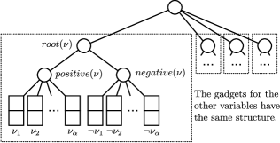
Figure 1: The construction of the variable gadget for $\nu$. If $\nu$ appears in the first clause, a chunk $c_{1}$, will be located at $\nu_{1}$. If $\neg\nu$ satisfies the last clause, $\neg\nu_{\alpha}$ will host $c_{\alpha}$.

For all variables $\nu$, we set the bandwidth on the link, connecting $root(\nu)$ to the root of the substrate tree, to $\alpha\cdot(\alpha\cdot\beta-\alpha)$. The bandwidth on the other edges is not limited.

We set the number of nodes to $n_{V}=\alpha\cdot\beta$. Moreover, we define the inter-connect communication cost to be $1$, and the access cost to be a sufficiently large constant $W$, such that nodes must always be collocated with chunks ($W=Th+1$ is sufficient).

We set the number of chunk types to be equal to the number of clauses, $\tau=\alpha$. To finish our construction, we place data chunks at leaves, as follows: for the $i$-th clause we construct as many replicas of chunk $c_{i}$ as there are literals in the clause. For each literal $\ell$ (of the form $\nu$ or $\neg\nu$) that satisfies clause $i$, we place a replica of chunk $c_{i}$ in the leaf labeled $\ell_{i}$.

Note, that in this construction some nodes will be idle. No chunks will be assigned to these nodes, but they will nevertheless participate in the node interconnect.

We set the threshold $Th$ to: $Th=\beta\cdot({\alpha\choose 2}\cdot 2+\alpha\cdot(\alpha\cdot\beta-\alpha))$.

Proof of correctness of construction. We now show that our construction indeed decides Sat. We set the capacities such that in every gadget, at most $\alpha$ nodes can be mapped, where $\alpha$ is the number of clauses of $\Psi$ . We can apply the Bandwidth Lemma (Lemma 6) as follows: We interpret $a_{i}$ as the number of nodes that are embedded in the $i$-th gadget, $\alpha$ as the number of clauses, and $\beta$ as the number of variables. The LHS of the inequality of Lemma 6 is a formula for the communication cost of nodes inside the $i$-th gadget to nodes outside the gadget. The RHS of the inequality is the bandwidth constraint for the gadget. This implies that any feasible solution must embed exactly $\alpha$ nodes in every gadget. Recall that in our Sat instance, we have at least four variables.

Theorem 1.

The problem EMB is NP-hard.

Proof.

We will prove that formula $\Psi$ is satisfiable iff EMB has a solution of cost $\leq Th$.

($\Rightarrow$) Let us take any valuation $Val$ that satisfies $\Psi$. We will construct a solution to EMB using $Val$ in the following way. For each variable $\nu$ in $\Psi$, we embed $\alpha$ many nodes at the leaves of the gadget of $\nu$. We need to choose $\alpha$ out of $2\cdot\alpha$ leaves to embed nodes. If $Val(\nu)=1$, we embed nodes at the leaves of $positive(\nu)$, else we embed all nodes at leaves $negative(\nu)$. The solution constructed this way has cost exactly $Th$, because the nodes are evenly split among gadgets, and nodes are not distributed across $positive(\nu)$ and $negative(\nu)$ subtrees.

We calculate the chunk-node matching $\mu$ by assigning every chunk to the node which is collocated with the first chunk replica. This solution is feasible because every clause of $\Psi$ was satisfied and chunks correspond to clauses.

Now we will show that this solution has cost $Th$. Due to the Bandwidth Lemma (Lemma 6), we only have to consider the communication cost. We sum inner-gadget communication and communication among gadgets to get exactly $Th$.

($\Leftarrow$) Let us take any solution to EMB constructed based on $\Psi$ of cost $\leq Th$. We will construct a positive valuation $Val$ by considering the nodes in the solution to EMB.

We make the following observations. In every solution of cost $\leq Th$, every gadget has exactly $\alpha$ many nodes at its leaves. This is due to the Bandwidth Lemma (Lemma 6). Also, inside every gadget either all nodes are in the $positive(\nu)$ subtree of variable $\nu$, or in the $negative(\nu)$ subtree. This is true because the cost of a solution where at least one gadget has nodes distributed across subtrees is always greater than $Th$.

Now we can construct our valuation $Val$, as follows (for each variable $\nu$ in $\Psi$): If $v_{1}$ hosts a node then $Val(\nu)=1$, otherwise $Val(\nu)=0$.

The valuation $Val$ satisfies all clauses, and hence $\Psi$, as the solution to EMB covers all chunks. To see this, consider the leaf which hosts a node which is assigned to any given chunk (i.e., the leaf handling any given clause chunk); it is a witness that the corresponding clause is satisfied.

∎

We conclude by observing that our construction leverages the fact that the number of nodes may exceed the number of chunk types, e.g., for a clause $(x\vee y\vee z)$ in $\Psi$, both $x$ and $y$ being true implies the mapping of nodes on vertices labeled $x_{1}$ and $y_{1}$, and which contain the same chunk $c_{1}$.

3.1 Hardness of problem with two replicas of each type

We can see that proof from previous section can be carried from 3SAT. This way we need only three replicas of each chunk type. 2SAT is not NP-hard, not allowing to carry previous construction for two replicas of each type. In this section we will show how to modify the construction to show NP-hardness of problem constrained to have at most two replicas of each type.

Our results so far indicate that dealing with replication can be challenging. However, all our hardness proofs concerned scenarios with three replicas, which raises the question whether the problems are solvable in polynomial time with a replication factor of $2$. (Similarly to, say, the 2-Sat problem which is tractable in contrast to 3-Sat.)

In the following, we show that this is not the case: the problem remains NP-hard, at least in the capacitated network.

The proof is by reduction from 3-Sat. Given a formula $\Psi$ in conjunctive normal form, consisting of $\alpha$ clauses and $\beta$ variables, we construct a problem instance and substrate tree $T_{\Psi}$ using two types of gadgets: gadgets for variables and gadgets for clauses. Nota bene: unlike in the previous proof we will create three chunk types instead of just one, for every clause.

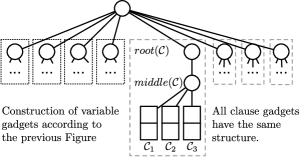
Figure 2: Structure of clause gadgets.

Construction. We build upon the construction for variable gadgets introduced (see also Figure 1).

1. Tree Construction: In addition to the variable gadgets known from the previous construction, we introduce clause gadgets. The clause gadget for a clause $\mathcal{C}$ (illustrated in Figure 2) has two inner vertices: root$(\mathcal{C})$, middle$(\mathcal{C})$ and three leaves $\mathcal{C}_{1},\mathcal{C}_{2}$ and $\mathcal{C}_{3}$ . We connect leaves to the middle vertex, and the middle vertex to root$(c)$. We attach the gadget to the tree by linking directly the global root to root$(\mathcal{C})$. We construct our tree out of $\beta$ variable gadgets and $\alpha$ clause gadgets.

2. Chunk Distribution: For each clause $\mathcal{C}$, we generate $3$ chunks types with $2$ replicas each. Each server in the clause gadget of $\mathcal{C}$ holds a replica of a different chunk type. The remaining replicas of chunk types, are placed in the variable gadgets of the variables which satisfy the clause, similarly to the previous proof. Thus, in total, $6\cdot\alpha$ variable chunks are distributed in the substrate network. We will consider a setting where $\alpha\cdot\beta+2\alpha$ nodes need to be mapped. Our intention is that in every variable gadget, there will be $\alpha$ nodes, and in every clause gadgets there will be two nodes.

3. Bandwidth Constraints: The available bandwidth of the top edge of the gadget of each variable $\nu$ is set to $\emph{cap}(\nu)=\alpha(\alpha(\beta-1)+2\cdot\alpha)$. This value, results from $\alpha$ nodes in the gadget for $\nu$, which each have to communicate to $\alpha\cdot(\beta-1)$ nodes in other variable gadgets and $2\cdot\alpha$ nodes in clause gadgets. The available bandwidth for the top edge of each clause gadget is set to $\emph{cap}(\alpha)=2(\alpha\cdot\beta+2(\alpha-1))$. This value allows both of the $2$ nodes in a clause gadget, to communicate to the $\alpha\cdot\beta$ nodes in variable gadgets and the the other $2(\alpha-1)$ nodes in clause gadgets.

4. Additional Properties: We set the threshold in a similar fashion as in previous proofs. That is, the threshold depends on the intra-clause communication cost ($2$ hops), and the inter-clause communication cost ($6$ hops). We set the number of nodes to be placed to $\alpha\cdot\beta+2\cdot\alpha$. We set the hosting capacity of each server to $1$, and set $b_{1}=Th+1$ to disallow remote chunk access. We set $b_{2}=1$.

Proof of correctness. We first prove the following helper lemma.

Lemma 2.

Every valid solution to EMB(2) with cost at most $Th$ has the property that there are exactly $\alpha$ nodes in each of the $\beta$ variable gadgets and exactly two nodes in each of the $\alpha$ clause gadgets.

Correctness follows from the extended bandwidth lemma (Lemma 7).

Theorem 3.

EMB(2) is NP-hard.

Proof.

We show that EMB(2) has a solution of cost $\leq Th$ if and only if $\Psi\in\textsc{3-Sat}$ is satisfiable.

($\Rightarrow$) If we have a positive valuation of $\Psi$, we fill variable gadgets with nodes like in the proofs before. Then we place $2$ nodes in each of the $\alpha$ clause gadgets as follows: Given a clause $\mathcal{C}=\ell_{1}\lor\ell_{2}\lor\ell_{3}$, we pick an arbitrary literal which satisfies the clause. Subsequently we place nodes at the leaf nodes in the clause gadget, which correspond to the other two literals. This strategy ensures that all chunks can be assigned to collocated nodes, as the only chunk type, which cannot be assigned to a collocated node in the clause gadget, has a node collocated with its second replica in the variable gadget.

We will then assign chunks to nodes in the following way: For chunk type we assign the replica in the variable gadgets to a collocated node. If this node does not exist, we assign the replica in the clause gadgets, to its collocated node.

Thus, we have produced a feasible solution of cost $Th$. ($\Leftarrow$) Let us take any solution $SOL$ to EMB(2) of cost $\leq Th$. Similar to the proof of Theorem 1 and Lemma 6 all nodes which are placed in a variable gadgets, will be located in either the positive or the negative subtree. Then we can compute a positive valuation by setting each variable $\nu$ as follows:

$Val(\nu)=\begin{cases}1&\mbox{iff there is a node at the first leaf}\\ &\mbox{on positive side of $\nu$ gadget in $SOL$}\\ 0&\mbox{otherwise}\end{cases}$

The theorem now follows from the following two additional lemmas.

Lemma 4.

For every clause there exists a node in a variable gadget that processes one of three chunks that correspond to that clause.

Proof.

Each of the three chunks that correspond to each clause, is assigned a collocated node. At least one of those three nodes is not idle in a variable gadget; otherwise, those two nodes in the clause gadgets would not suffice in satisfying all chunk types. ∎

Observe that it might happen that in $SOL$, two nodes in clause variables are idle, and three nodes in variable gadgets are processing those $3$ chunk types. In this case, arbitrary nodes can be taken for the rest of the proof.

Lemma 5.

$Val$ satisfies $\Psi$.

Proof.

Let us consider the matching $M$ of $SOL$, and let us consider an arbitrary clause of $\Psi$ as well as its three chunk types: Due to bandwidth constraints, at most two of the chunks types, can be processed by nodes in the clause gadgets. We identify any chunk type, which is not assigned to a replica in the clause gadgets. The processed replica of that chunk type was located in a variable gadget. Depending on whether the replica was located in the positive or the negative subtree, we set the value of the according variable to $1$ (positive subtree) or $0$ (negative subtree). ∎

∎

4 The Bandwidth Lemmas

Lemma 6 (Bandwidth Lemma).

Let $\alpha$ and $\beta>4$ be two arbitrary positive integers. Let $a_{1},a_{2},\ldots,a_{\beta}$ be a sequence of $\beta$ integers which adds up to $\alpha\cdot\beta$. Also, for each $i$ we have $a_{i}\leq 2\cdot\alpha$. Then it holds that if

$$\forall_{i}:~{}~{}a_{i}\cdot(\alpha\cdot\beta-a_{i})\leq\alpha\cdot(\alpha\cdot\beta-\alpha),$$

then for each $i$: $a_{i}=\alpha$.

Proof.

By contradiction. Let us assume that there exists an index $k$ such that $a_{k}\neq\alpha$. Then we can distinguish between two cases: either $a_{k}<\alpha$ or $a_{k}>\alpha$.

Case $a_{k}<\alpha$: If there exists a $k$ with $a_{k}<\alpha$, due to the fact that the sequence adds up to $\alpha\cdot\beta$, there must also exist a $k^{\prime}$ such that $a_{k^{\prime}}<\alpha$ (by a simple pigeon hole principle). Thus, this case can also be reduced to the second case (Case $a_{k}>\alpha$) proved next.

Case $a_{k}>\alpha$: Since it also holds that $a_{k}<2\alpha$, $a_{k}$ must be of the form $\alpha+x$ for $x\in[1,\ldots,\alpha]$. Let us consider the (bandwidth) inequality:

$$(\alpha+x)\cdot(\alpha\cdot\beta-\alpha-x)\leq\alpha\cdot(\alpha\cdot\beta-x)$$

This can be transformed to:

$$0\leq x(x-(\alpha\cdot(\beta-2)))$$

The equation holds for $x\leq 0$ or $x\geq\alpha\cdot(\beta-2)$, and no positive $x\leq\alpha$ can satisfy this inequality for $\beta>4$. Contradiction. ∎

Lemma 7 (Extended Bandwidth Lemma).

Let $\alpha$ and $\beta>4$ be two arbitrary positive integers. Let $a_{1},a_{2},\ldots,a_{\alpha}$ and $b_{1},b_{2},\ldots,b_{\beta}$ be two sequences of integers (numbers of nodes in clause and in variable gadgets). The sum of all elements in $a$ and $b$ adds up to $\alpha\cdot\beta+\alpha\cdot 2$ (number of nodes). Also we have $a_{i}\leq 2\cdot\alpha$ (variable gadget node hosting capacity – equal to number of leaves), and $b_{i}\leq 3$ (clause gadget node hosting capacity). If uplink of variable gadget does not exceed bandwidth constraints

$$\forall_{i\leq\beta}:~{}~{}b_{i}\cdot(\alpha\cdot\beta+2\cdot\alpha-b_{i})\leq\alpha\cdot(\alpha\cdot\beta-\alpha+2\cdot\alpha),$$

and uplink of clause gadget does not exceed bandwidth constraints

$$\forall_{i\leq\alpha}:~{}~{}a_{i}\cdot(\alpha\cdot\beta+2\cdot\alpha-a_{i})\leq 2\cdot(\alpha\cdot\beta-2\cdot\alpha-2),$$

then for each $i\leq\beta$: $b_{i}=\alpha$ and for each $i\leq\alpha$: $a_{i}=2$ (we have expected number of nodes in variable and clause gadgets).

We can prove the extended bandwidth lemma by pidgeon hole principle. However, easier way exists. We sum available bandwidth on all uplinks of clause gadgets to $C$ and bandwidth an uplinks of variable gadgets to $V$. The only way that we can distribute nodes between clause and variable gadgets is to have $2\cdot\alpha$ in total in clause gadgets and $\alpha\cdot\beta$ in variable gadgets. To conclude, we apply bandwidth lemma 6 to clause gadgets and separatly to variable gadgets.

5 Related Work

There has recently been much interest in programming models and distributed system architectures for the processing and analysis of big data (e.g. [2, 6, 17]). The model studied in this paper is motivated by MapReduce [6] like batch-processing applications, also known from the popular open-source implementation Apache Hadoop. These applications generate large amounts of network traffic [4, 10, 18], and over the last years, several systems have been proposed which provide a provable network performance, also in shared cloud environments, by supporting relative [11, 12, 15] or, as in the case of our paper, absolute [3, 9, 13, 14, 16] bandwidth reservations between the virtual machines.

The most popular virtual network abstraction for batch-processing applications today is the virtual cluster, introduced in the Oktopus paper [3], and later studied by many others [10, 16]. Several heuristics have been developed to compute ’’good‘‘ embeddings of virtual clusters: embeddings with small footprints (minimal bandwidth reservation costs) [3, 10, 16]. The virtual network embedding problem has also been studied for more general graph abstractions (e.g., motivated by wide-area networks). [5, 7]

6 Summary and Conclusion

We shown that several embedding problems are NP-hard already in three-level trees—a practically relevant result given today‘s datacenter topologies [1])—and even if the the number of replicas is bounded by two.

References

- [1] M. Al-Fares, A. Loukissas, and A. Vahdat. A scalable, commodity data center network architecture. In Proc. ACM SIGCOMM, pages 63–74, 2008.
- [2] I. Alagiannis, R. Borovica, M. Branco, S. Idreos, and A. Ailamaki. Nodb: Efficient query execution on raw data files. In Proc. ACM SIGMOD, pages 241–252, 2012.
- [3] H. Ballani, P. Costa, T. Karagiannis, and A. Rowstron. Towards predictable datacenter networks. In Proc. ACM SIGCOMM, 2011.
- [4] M. Chowdhury, M. Zaharia, J. Ma, M. I. Jordan, and I. Stoica. Managing Data Transfers in Computer Clusters with Orchestra. In Proc. ACM SIGCOMM, 2011.
- [5] N. M. K. Chowdhury and R. Boutaba. A survey of network virtualization. Comput. Netw., 54(5):862–876, 2010.
- [6] J. Dean and S. Ghemawat. Mapreduce: Simplified data processing on large clusters. In Proc. USENIX OSDI, pages 137–150, 2004.
- [7] A. Fischer, J. Botero, M. Beck, H. DeMeer, and X. Hesselbach. Virtual network embedding: A survey. 2013.
- [8] A. Greenberg, J. R. Hamilton, N. Jain, S. Kandula, C. Kim, P. Lahiri, D. A. Maltz, P. Patel, and S. Sengupta. VL2: a scalable and flexible data center network. In Proc. ACM SIGCOMM, 2009.
- [9] C. Guo, G. Lu, H. J. Wang, S. Yang, C. Kong, P. Sun, W. Wu, and Y. Zhang. SecondNet: A data center network virtualization architecture with bandwidth guarantees. In Proc. 6th CoNEXT, 2010.
- [10] J. C. Mogul and L. Popa. What we talk about when we talk about cloud network performance. ACM SIGCOMM Computer Communication Review (CCR), 2012.
- [11] L. Popa, A. Krishnamurthy, S. Ratnasamy, and I. Stoica. Faircloud: Sharing the network in cloud computing. In Proc. HotNets-X, 2011.
- [12] L. Popa, P. Yalagandula, S. Banerjee, J. C. Mogul, Y. Turner, and J. R. Santos. Elasticswitch: Practical work-conserving bandwidth guarantees for cloud computing. In Proc. ACM SIGCOMM, pages 351–362, 2013.
- [13] B. Raghavan, K. Vishwanath, S. Ramabhadran, K. Yocum, and A. C. Snoeren. Cloud control with distributed rate limiting. In Proc. SIGCOMM, pages 337–348, 2007.
- [14] H. Rodrigues, J. R. Santos, Y. Turner, P. Soares, and D. Guedes. Gatekeeper: Supporting bandwidth guarantees for multi-tenant datacenter networks. In Proc. 3rd Conference on I/O Virtualization (WIOV), 2011.
- [15] A. Shieh, S. Kandula, A. Greenberg, and C. Kim. Seawall: Performance isolation for cloud datacenter networks. In Proc. USENIX HotCloud, 2010.
- [16] D. Xie, N. Ding, Y. C. Hu, and R. Kompella. The only constant is change: incorporating time-varying network reservations in data centers. ACM SIGCOMM Computer Communication Review (CCR), 2012.
- [17] R. S. Xin, J. Rosen, M. Zaharia, M. J. Franklin, S. Shenker, and I. Stoica. Shark: Sql and rich analytics at scale. In Proce. ACM SIGMOD, pages 13–24, 2013.
- [18] Measuring EC2 system performance. http://goo.gl/V5zhEd.