Decay bounds for functions of matrices with banded or Kronecker structure

Abstract

We present decay bounds for a broad class of Hermitian matrix functions where the matrix argument is banded or a Kronecker sum of banded matrices. Besides being significantly tighter than previous estimates, the new bounds closely capture the actual (non-monotonic) decay behavior of the entries of functions of matrices with Kronecker sum structure. We also discuss extensions to more general sparse matrices.

1 Introduction

The decay behavior of the entries of functions of banded and sparse matrices has attracted considerable interest over the years. It has been known for some time that if $A$ is a banded Hermitian matrix and $f$ is a smooth function with no singularities in a neighborhood of the spectrum of $A$, then the entries in $f(A)$ usually exhibit rapid decay in magnitude away from the main diagonal. The decay rates are typically exponential, with even faster decay in the case of entire functions.

The interest for the decay behavior of matrix functions stems largely from its importance for a number of applications including numerical analysis [6, 12, 15, 16, 21, 39, 45], harmonic analysis [2, 25, 32], quantum chemistry [5, 10, 36, 41], signal processing [34, 42], quantum information theory [13, 14, 22], multivariate statistics [1], queueing models [9], control of large-scale dynamical systems [28], quantum dynamics [24], random matrix theory [40], and others. The first case to be analyzed in detail was that of $f(A)=A^{-1}$, see [16, 17, 21, 33]. In these papers one can find exponential decay bounds for the entries of the inverse of banded matrices. A related, but quite distinct line of research concerned the study of inverse-closed matrix algebras, where the decay behavior in the entries of a (usually infinite) matrix $A$ is “inherited” by the entries of $A^{-1}$. Here we mention [32], where it was observed that a similar decay behavior occurs for the entries of $f(A)=A^{-1/2}$, as well as [2, 3, 25, 26, 34], among others.

The study of the decay behavior for general analytic functions of banded matrices, including the important case of the matrix exponential, was initiated in [6, 31] and continued for possibly non-normal matrices and general sparsity patterns in [7]; further contributions in these directions include [4, 15, 37, 41]. Collectively, these papers have largely elucidated the question of when one can expect exponential decay in the entries of $f(A)$, in terms of conditions that the function $f$ and the matrix $A$ must satisfy. Some of these papers also address the important problem of when the rate of decay is asymptotically independent of the dimension $n$ of the problem, a condition that allows, at least in principle, for the approximation of $f(A)$ with a computational cost scaling linearly in $n$ (see, e.g., [5, 7, 10]).

A limitation of these papers is that they provide decay bounds for the entries of $f(A)$ that are often pessimistic and may not capture the correct, non-monotonic decay behavior actually observed in many situations of practical interest. A first step to address this issue was taken in [11], where new bounds for the inverses of matrices that are Kronecker sums of banded matrices (a kind of structure of considerable importance in the numerical solution of PDE problems) were obtained; see also [39] for an early such analysis for a special class of matrices, and [37] for functions of multiband matrices.

In this paper we build on the work in [11] to investigate the decay behavior in (Hermitian) matrix functions where the matrix is a Kronecker sum of banded matrices. We also present new bounds for functions of banded (more generally, sparse) Hermitian matrices. For certain broad classes of analytic functions that frequently arise in applications (including as special cases the resolvent, the inverse square root, and the exponential) we obtain improved decay bounds that capture much more closely the actual decay behavior of the matrix entries than previously published bounds. A significant difference with previous work in this area is that our bounds are expressed in integral form, and in order to apply the bounds to specific matrix functions it may be necessary to evaluate these integrals numerically.

The paper is organized as follows. In section 2 we provide basic definitions and material from linear algebra and analysis utilized in the rest of the paper. In section 3 we briefly recall earlier work on decay bounds for matrix functions. New decay results for functions of banded matrices are given in section 4. Generalizations to more general sparse matrices are briefly discussed in section 5. Functions of matrices with Kronecker sum structure are treated in section 6. Conclusive remarks are given in section 7.

2 Preliminaries

In this section we give some basic definitions and background information on the types of matrices and functions considered in the paper.

2.1 Banded matrices and Kronecker sums

We begin by recalling two standard definitions.

Definition 1.

We say that a matrix $M\in{\mathbb{C}}^{n\times n}$ is $\beta$-banded if its entries $M_{ij}$ satisfy $M_{ij}=0$ for $|i-j|>\beta$.

Definition 2.

Let $M_{1},M_{2}\in{\mathbb{C}}^{n\times n}$. We say that a matrix ${\cal A}\in{\mathbb{C}}^{n^{2}\times n^{2}}$ is the Kronecker sum of $M_{1}$ and $M_{2}$ if

$${\cal A}=M_{1}\oplus M_{2}:=M_{1}\otimes I+I\otimes M_{2}\,,$$ (1)

where $I$ denotes the $n\times n$ identity matrix.

In this paper we will be especially concerned with the case $M_{1}=M_{2}=M$, where $M$ is $\beta$-banded and Hermitian positive definite (HPD). In this case $\cal A$ is also HPD.

The definition of Kronecker sum can easily be extended to three or more matrices. For instance, we can define

$${\cal A}=M_{1}\oplus M_{2}\oplus M_{3}:=M_{1}\otimes I\otimes I+I\otimes M_{2}\otimes I+I\otimes I\otimes M_{3}.$$

The Kronecker sum of two matrices is well-behaved under matrix exponentiation. Indeed, the following relation holds (see, e.g., [29, Theorem 10.9]):

$$\exp(M_{1}\oplus M_{2})=\exp(M_{1})\otimes\exp(M_{2}).$$ (2)

Similarly, the following matrix trigonometric identities hold for the matrix sine and cosine [29, Theorem 12.2]:

$$\sin(M_{1}\oplus M_{2})=\sin(M_{1})\otimes\cos(M_{2})+\cos(M_{1})\otimes\sin(M_{2})$$ (3)

and

$$\cos(M_{1}\oplus M_{2})=\cos(M_{1})\otimes\cos(M_{2})-\sin(M_{1})\otimes\sin(M_{2}).$$ (4)

As we will see, identity (2) will be useful in extending decay results for functions of banded matrices to functions of matrices with Kronecker sum structure.

2.2 Classes of functions defined by integral transforms

We will be concerned with analytic functions of matrices. It is well known that if $f$ is a function analytic in a domain $\Omega\subseteq{\mathbb{C}}$ containing the spectrum of a matrix $A\in{\mathbb{C}}^{n\times n}$, then

$$f(A)=\frac{1}{2\pi i}\int_{\Gamma}f(z)(zI-A)^{-1}{\rm d}z\,,$$ (5)

where $i=\sqrt{-1}$ is the imaginary unit and $\Gamma$ is any simple closed curve surrounding the eigenvalues of $A$ and entirely contained in $\Omega$, oriented counterclockwise.

Our main results concern certain analytic functions that can be represented as integral transforms of measures, in particular, strictly completely monotonic functions (associated with the Laplace–Stieltjes transform) and Markov functions (associated with the Cauchy–Stieltjes transform). Here we briefly review some basic properties of these functions and the relationship between the two classes. We begin with the following definition (see [44]).

Definition 3.

Let $f$ be defined in the interval $(a,b)$ where $-\infty\leq a<b\leq+\infty$. Then, $f$ is said to be completely monotonic in $(a,b)$ if

$$(-1)^{k}f^{(k)}(x)\geq 0\quad{\rm for\ all}\quad a<x<b\quad{\rm and\ all}\quad k=0,1,2,\ldots$$

Moreover, $f$ is said to be strictly completely monotonic in $(a,b)$ if

$$(-1)^{k}f^{(k)}(x)>0\quad{\rm for\ all}\quad a<x<b\quad{\rm and\ all}\quad k=0,1,2,\ldots$$

Here $f^{(k)}$ denotes the $k$th derivative of $f$, with $f^{(0)}\equiv f$. It is shown in [44] that if $f$ is completely monotonic in $(a,b)$, it can be extended to an analytic function in the open disk $|z-b|<b-a$ when $b$ is finite. When $b=+\infty$, $f$ is analytic in $\Re(z)>a$. Therefore, for each $y\in(a,b)$ we have that $f$ is analytic in the open disk $|z-y|<R(y)$, where $R(y)$ denotes the radius of convergence of the power series expansion of $f$ about the point $z=y$. Clearly, $R(y)\geq y-a$ for $y\in(a,b)$.

In [8] Bernstein proved that a function $f$ is completely monotonic in $(0,\infty)$ if and only if $f$ is the Laplace–Stieltjes transform of $\alpha(\tau)$;

$$f(x)=\int_{0}^{\infty}{\rm e}^{-\tau x}{\rm d}\alpha(\tau),$$ (6)

where $\alpha(\tau)$ is nondecreasing and the integral in (6) converges for all $x>0$. Moreover, under the same assumptions $f$ can be extended to an analytic function on the positive half-plane $\Re(z)>0$. A refinement of this result (see [20]) states that $f$ is strictly completely monotonic in $(0,\infty)$ if it is completely monotonic there and moreover the function $\alpha(\tau)$ has at least one positive point of increase, that is, there exists a $\tau_{0}>0$ such that $\alpha(\tau_{0}+\delta)>\alpha(\tau_{0})$ for any $\delta>0$.

Prominent examples of strictly completely monotonic functions include (see [43]):

1. $f_{1}(x)=1/x=\int_{0}^{\infty}{\rm e}^{-x\tau}d\alpha_{1}(\tau)$ for $x>0$, where $\alpha_{1}(\tau)=\tau$ for $\tau\geq 0$.

2. $f_{2}(x)={\rm e}^{-x}=\int_{0}^{\infty}{\rm e}^{-x\tau}d\alpha_{2}(\tau)$ for $x>0$, where $\alpha_{2}(\tau)=0$ for $0\leq\tau<1$ and $\alpha_{2}(\tau)=1$ for $\tau\geq 1$.

3. $f_{3}(x)=(1-{\rm e}^{-x})/x=\int_{0}^{\infty}{\rm e}^{-x\tau}d\alpha_{3}(\tau)$ for $x>0$, where $\alpha_{3}(\tau)=\tau$ for $0\leq\tau\leq 1$, and $\alpha_{3}(\tau)=1$ for $\tau\geq 1$.

Other examples include the functions $x^{-\sigma}$ (for any $\sigma>0$), $\log(1+1/x)$ and $\exp(1/x)$, all strictly completely monotonic on $(0,\infty)$. Also, products and positive linear combinations of strictly completely monotonic functions are strictly completely monotonic, as one can readily check.

A closely related class of functions is given by the Cauchy–Stieltjes (or Markov-type) functions, which can be written as

$$f(z)=\int_{\Gamma}\frac{{\rm d}\gamma(\omega)}{z-\omega},\quad z\in{\mathbb{C}}\setminus\Gamma\,,$$ (7)

where $\gamma$ is a (complex) measure supported on a closed set $\Gamma\subset{\mathbb{C}}$ and the integral is absolutely convergent. In this paper we are especially interested in the special case $\Gamma=(-\infty,0]$ so that

$$f(x)=\int_{-\infty}^{0}\frac{{\rm d}\gamma(\omega)}{x-\omega},\quad x\in{\mathbb{C}}\setminus(-\infty,0]\,,$$

where $\gamma$ is now a (possibly signed) real measure. The following functions, which occur in various applications (see, e.g., [27] and references therein), fall into this class:

$$z^{-\frac{1}{2}}=\int_{-\infty}^{0}\frac{1}{z-\omega}\frac{1}{\pi\sqrt{-\omega}}{\rm d}\omega,$$

$$\frac{{\rm e}^{-t\sqrt{z}}-1}{z}=\int_{-\infty}^{0}\frac{1}{z-\omega}\frac{\sin(t\sqrt{-\omega})}{-\pi\omega}{\rm d}\omega,$$

$$\frac{\log(1+z)}{z}=\int_{-\infty}^{-1}\frac{1}{z-\omega}\frac{1}{(-\omega)}{\rm d}\omega.$$

The two classes of functions just introduced overlap. Indeed, it is easy to see (e.g., [38]) that functions of the form

$$f(x)=\int_{0}^{\infty}\frac{{\rm d}\mu(s)}{x+\omega},$$

with $\mu$ a positive measure, are strictly completely monotonic on $(0,\infty)$; but every such function can also be written in the form

$$f(x)=\int_{-\infty}^{0}\frac{{\rm d}\gamma(\omega)}{x-\omega},\quad\gamma(\omega)=-\mu(-\omega),$$

and therefore it is a Cauchy–Stieltjes function. We note that $f(x)=\exp(-x)$ is an example of a function that is strictly completely monotonic but not a Cauchy–Stieltjes function.

In the rest of the paper, the term Laplace–Stieltjes function will be used to denote a function that is strictly completely monotonic on $(0,\infty)$.

3 Previous work

In this section we briefly review some previous decay results from the literature.

Given a $n\times n$ Hermitian positive definite $\beta$-banded matrix $M$, it was shown in [17] that

$$|(M^{-1})_{ij}|\leq Cq^{\frac{|i-j|}{\beta}}$$ (8)

for all $i,j=1,\ldots,n$, where $q=(\sqrt{\kappa}-1)/(\sqrt{\kappa}+1)$, $\kappa$ is the spectral condition number of $M$, $C=\max\{1/\lambda_{\rm min}(M),\hat{C}\}$, and $\hat{C}=(1+\sqrt{\kappa})^{2}/(2\lambda_{\max}(M))$. In this bound the diagonal elements of $M$ are assumed not to be greater than one, which can always be satisfied by dividing $M$ by its largest diagonal entry, after which the bound (8) will have to be multiplied by its reciprocal. The bound is known to be sharp, in the sense that it is attained for a certain tridiagonal Toeplitz matrix. We mention that (8) is also valid for infinite and bi-infinite matrices as long as they have finite condition number, i.e., both $M$ and $M^{-1}$ are bounded. Using the identity $M^{-1}=(M^{*}M)^{-1}M^{*}$, simple decay bounds were also obtained in [17] for non-Hermitian matrices.

Similarly, if $M$ is $\beta$-banded and Hermitian and $f$ is analytic on a region of the complex plane containing the spectrum $\sigma(M)$ of $M$, then there exist positive constants $C$ and $q<1$ such that

$$|(f(M))_{ij}|\leq Cq^{\frac{|i-j|}{\beta}},$$ (9)

where $C$ and $q$ can be expressed in terms of the parameter of a certain ellipse surrounding $\sigma(M)$ and of the maximum modulus of $f$ on this ellipse; see [6]. The bound (9), in general, is not sharp; in fact, since there are infinitely many ellipses containing $\sigma(M)$ in their interior and such that $f$ is analytic inside the ellipse and continuous on it, one should think of (9) as a parametric family of bounds rather than a single bound. By tuning the parameter of the ellipse one can obtain different bounds, usually involving a trade-off between the values of $C$ and $q$. This result was extended in [7] to the case where $M$ is a sparse matrix with a general sparsity pattern, using the graph distance instead of the distance from the main diagonal; see also [13, 32] and section 5 below. Similar bounds for analytic functions of non-Hermitian matrices can be found in [4, 7].

Practically all of the above results consist of exponential decay bounds on the magnitude of the entries of $f(M)$. However, for entire functions the actual decay is typically superexponential, rather than exponential. Such bounds have been obtained by Iserles for the exponential of a tridiagonal matrix in [31]. This paper also presents superexponential decay bounds for the exponential of banded matrices, but the bounds only apply at sufficiently large distances from the main diagonal. None of these bounds require $M$ to be Hermitian. Superexponential decay bounds for the exponential of certain infinite tridiagonal skew-Hermitian matrices arising in quantum mechanical computations have been recently obtained in [41].

4 Decay estimates for functions of a banded matrix

In this section we present new decay bounds for functions of matrices $f(M)$ where $M$ is a banded, Hermitian and positive definite. First, we make use of an important result from [30] to obtain decay bounds for the entries of the exponential of a banded, Hermitian, positive semidefinite matrix $M$. This result will then be used to obtain bounds or estimates on the entries of $f(M)$, where $f$ is strictly completely monotonic. In a similar manner, we will obtain bounds or estimates on the entries of $f(M)$ where $f$ is a Markov function by making use of the classical bounds of Demko et al. [17] for the entries of the inverses of banded positive definite matrices.

In section 6 we will use these results to obtain bounds for matrix functions $f({\cal A})$, where $\cal A$ is a Kronecker sum of banded matrices and $f$ belongs to one of the two above-mentioned classes of functions.

4.1 The exponential of a banded Hermitian matrix

We first recall (with a slightly different notation) an important result due to Hochbruck and Lubich [30]. Here the $m$ columns of $V_{m}\in{\mathbb{C}}^{n\times n}$ form an orthonormal basis for the Krylov subspace $K_{m}(M,v)={\rm span}\{v,Mv,\ldots,M^{m-1}v\}$ with $\|v\|=1$, and $H_{m}=V_{m}^{*}MV_{m}$.

Theorem 4.

Let $M$ be a Hermitian positive semidefinite matrix with eigenvalues in the interval $[0,4\rho]$. Then the error in the Arnoldi approximation of $\exp(\tau M)v$ with $\|v\|=1$, namely $\varepsilon_{m}:=\|\exp(-\tau M)v-V_{m}\exp(-\tau H_{m})e_{1}\|$, is bounded in the following ways:

1. $\varepsilon_{m}\leq 10\exp(-m^{2}/(5\rho\tau))$, for $\rho\tau\geq 1$ and $\sqrt{4\rho\tau}\leq m\leq 2\rho\tau$

2. $\varepsilon_{m}\leq 10(\rho\tau)^{-1}\exp(-\rho\tau)\left(\frac{{\rm e}\rho\tau}{m}\right)^{m}$ for $m\geq 2\rho\tau$.

With this result we can establish bounds for the entries of the exponential of a banded Hermitian matrix.

Theorem 5.

Let $M$ be as in Theorem 4. Assume in addition that $M$ is $\beta$-banded. Then, with the notation of Theorem 4 and for $k\neq t$:

1. For $\rho\tau\geq 1$ and $\sqrt{4\rho\tau}\leq|k-t|/\beta\leq 2\rho\tau$,

   $$|(\exp(-\tau M))_{kt}|\leq 10\exp\left(-\frac{(|k-t|/\beta)^{2}}{5\rho\tau}\right);$$

2. For $|k-t|/\beta\geq 2\rho\tau$,

   $$|(\exp(-\tau M))_{kt}|\leq 10\frac{\exp(-\rho\tau)}{\rho\tau}\left(\frac{{\rm e}\rho\tau}{\frac{|k-t|}{\beta}}\right)^{\frac{|k-t|}{\beta}}.$$

Proof.

We first note that an element of the Krylov subspace $K_{m}(M,v)$ is a polynomial in $M$ times a vector, so that $V_{m}\exp(-\tau H_{m})e_{1}=p_{m-1}(\tau M)v$ for some polynomial $p_{m-1}$ of degree at most $m-1$. Because $M$ is Hermitian and $\beta$-banded, the matrix $p_{m-1}(\tau M)$ is at most $(m-1)\beta$-banded.

Let now $k,t$ with $k\neq t$ be fixed, and write $|k-t|=(m-1)\beta+s$ for some $m\geq 1$ and $s=1,\ldots,\beta$; in particular, we see that $(p_{m-1}(\tau M))_{kt}=0$, moreover $|k-t|/\beta\leq m$. Consider first case ii). If $m\geq 2\rho\tau$, for $v=e_{t}$ we obtain

$$|(\exp(-\tau M))_{kt}| = |(\exp(-\tau M))_{kt}-(p_{m-1}(\tau M))_{kt}|$$

$$= |e_{k}^{T}(\exp(-\tau M)e_{t}-p_{m-1}(\tau M)e_{t})|$$

$$\leq \|\exp(-\tau M)e_{t}-p_{m-1}(\tau M)e_{t}\|$$

$$\leq 10(\rho\tau)^{-1}\exp(-\rho\tau)\left(\frac{e\rho\tau\beta}{|k-t|}\right)^{\frac{|k-t|}{\beta}},$$

where in the last inequality Theorem 4 was used for $m|k-t|/\beta\geq 2\rho\tau$. An analogous result is obtained for $m$ in the finite interval, so as to verify i). ∎

As remarked in [30], the restriction to positive semidefinite $M$ leads to no loss of generality, since a shift from $M$ to $M+\delta I$ entails a change by a factor ${\rm e}^{\tau\delta}$ in the quantities of interest.

We also notice that in addition to Theorem 4 other asymptotic bounds exist for estimating the error in the exponential function with Krylov subspace approximation; see, e.g., [18, 19]. An advantage of Theorem 4 is that it provides explicit upper bounds, which can then be easily used for our purposes.

Example 6.

Figure 1 shows the behavior of the bound in Theorem 5 for two typical matrices. The plot on the left refers to the tridiagonal matrix $M={\rm tridiag}(-1,4,-1)$ ($\beta=1$) of size $n=200$, with $\tau=4$, so that $\tau\rho\approx 3.9995$. The $t$th column with $t=127$ is reported, and only the values above $10^{-60}$ are shown. The plot on the right refers to the pentadiagonal matrix $M={\rm pentadiag}(-0.5,-1,4,-1,-0.5)$ ($\beta=2$) of size $n=200$, with $\tau=4$, so that $\tau\rho\approx 4.4989$. The same column $t=127$ is shown. Note the superexponential decay behavior. In both cases, the estimate seems to be rather sharp.

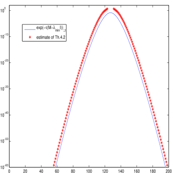
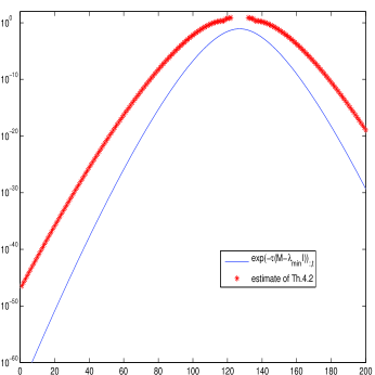
Fig. 1: Example 6. Bounds for $|\exp(-\tau(M-\lambda_{\min}I))|_{:,t}$, $t=127$, using Theorem 5. $M$ of size $n=200$ and $\tau=4$. Left: $M={\rm tridiag}(-1,4,-1)$. Right: $M={\rm pentadiag}(-0.5,-1,4,-1,-0.5)$. Logarithmic scale.

4.2 Bounds for Laplace–Stieltjes functions

By exploiting the connection between the exponential function and Laplace–Stieltjes functions, we can apply Theorem 5 to obtain bounds or estimates for the entries of Laplace–Stieltjes matrix functions.

Theorem 7.

Let $M=M^{*}$ be $\beta$-banded and positive definite, and let $\widehat{M}=M-\lambda_{\min}I$, with the spectrum of $\widehat{M}$ contained in $[0,4\rho]$. Assume $f$ is a Laplace–Stieltjes function, so that it can be written in the form $f(x)=\int_{0}^{\infty}{\rm e}^{-x\tau}{\rm d}\alpha(\tau)$. Then, with the notation and assumptions of Theorem 5 and for $|k-t|/\beta\geq 2$:

$$|f(M)|_{k,t} \leq \int_{0}^{\infty}\exp(-\lambda_{\min}\tau)|(\exp(-\tau\widehat{M}))_{k,t}|{\rm d}\alpha(\tau)$$

$$\leq 10\int_{0}^{\frac{|k-t|}{2\rho\beta}}\exp(-\lambda_{\min}\tau)\frac{\exp(-\rho\tau)}{\rho\tau}\left(\frac{{\rm e}\rho\tau}{\frac{|k-t|}{\beta}}\right)^{\frac{|k-t|}{\beta}}{\rm d}\alpha(\tau)$$

$$\quad+10\int_{\frac{|k-t|}{2\rho\beta}}^{\frac{|k-t|^{2}}{4\rho\beta^{2}}}\exp(-\lambda_{\min}\tau)\exp\left(-\frac{(|k-t|/\beta)^{2}}{5\rho\tau}\right){\rm d}\alpha(\tau)$$

$$+\int_{\frac{|k-t|^{2}}{4\rho\beta^{2}}}^{\infty}\exp(-\lambda_{\min}\tau)(\exp(-\tau\widehat{M}))_{k,t}{\rm d}\alpha(\tau)=I+II+III.$$

In general, these integrals may have to be evaluated numerically. We observe that in the above bound, the last term (III) does not significantly contribute provided that $|k-t|$ is sufficiently large while $\rho$ and $\beta$ are not too large.

As an illustration, consider the function $f(x)=1/\sqrt{x}$. For this function we have $\alpha(\tau)=\frac{1}{\sqrt{\tau}}\Gamma(-\frac{1}{2}+1)=\sqrt{\pi/\tau}$ with $\tau\in(0,\infty)$. We have

$$I+II = 10\sqrt{\pi}\int_{0}^{\frac{|k-t|}{2\rho\beta}}\frac{\exp(-\lambda_{\min}\tau)}{\tau\sqrt{\tau}}\frac{\exp(-\rho\tau)}{\rho\tau}\left(\frac{{\rm e}\rho\tau}{\frac{|k-t|}{\beta}}\right)^{\frac{|k-t|}{\beta}}{\rm d}\tau$$

$$+10\sqrt{\pi}\int_{\frac{|k-t|}{2\rho\beta}}^{\frac{|k-t|^{2}}{4\rho\beta^{2}}}\frac{\exp(-\lambda_{\min}\tau)}{\tau\sqrt{\tau}}\exp\left(-\frac{(|k-t|/\beta)^{2}}{5\rho\tau}\right){\rm d}\tau,$$

while

$$III\leq\sqrt{\pi}\int_{\frac{|k-t|^{2}}{4\rho\beta^{2}}}^{\infty}\frac{\exp(-\lambda_{\min}\tau)}{\tau\sqrt{\tau}}{\rm d}\tau.$$

Figure 2 shows two typical bounds for the entries of $M^{-\frac{1}{2}}$ for the same matrices $M$ considered in Example 6. The integrals $I$ and $II$ and the one appearing in the upper bound for $III$ have been evaluated accurately using the built-in Matlab function quad. Note that the decay is now exponential. In both cases, the decay is satisfactorily captured.

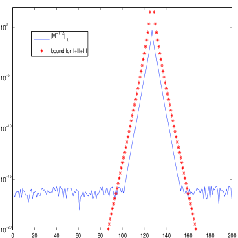
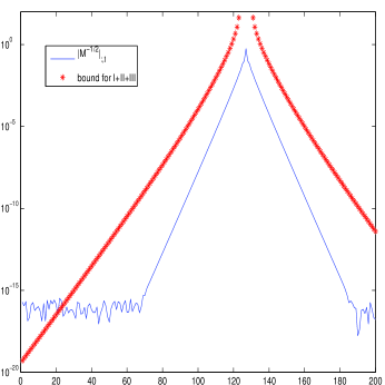
Fig. 2: Estimates for $|M^{-1/2}|_{:,t}$, $t=127$, using I+II and the upper bound for III. Size $n=200$, Log-scale. Left: $M={\rm tridiag}(-1,4,-1)$. Right: $M={\rm pentadiag}(-0.5,-1,4,-1,-0.5)$.

As yet another example, consider the entire function $f(x)=(1-\exp(-x))/x$ for $x\in[0,1]$, which is a Laplace–Stieltjes function with ${\rm d}\alpha(\tau)={\rm d}\tau$ (see section 2.2). Starting from (7) we can determine new terms $I,II$, and estimate $III$ as it was done for the inverse square root. Due to the small interval size, the first term $I$ accounts for the whole bound for most choices of $k,t$. For the same two matrices used above, the actual (superexponential) decay and its approximation are reported in Figure 3.

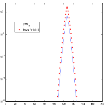
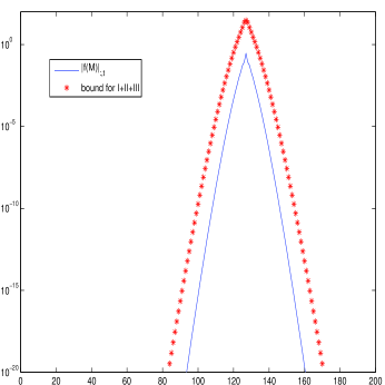
Fig. 3: Estimates for $|M^{-1}(I-\exp(-M))|_{:,t}$, $t=127$, using I+II and the upper bound for III. size $n=200$, Log-scale. Left: $M={\rm tridiag}(-1,4,-1)$. Right: $M={\rm pentadiag}(-0.5,-1,4,-1,-0.5)$.

We remark that for the validity of Theorem 7, we cannot relax the assumption that $M$ be positive definite. This makes sense since we are considering functions of $M$ that are defined on $(0,\infty)$. If $M$ is not positive definite but $f$ happens to be defined on a larger interval containing the spectrum of $M$, for instance on all of ${\mathbb{R}}$, it may still be possible, in some cases, to obtain bounds for $f(M)$ from the corresponding bounds on $f(M+\delta I)$ where the shifted matrix $M+\delta I$ is positive definite.

Remark 8.

We observe that if $f(M+i\zeta I)$ is well defined for $\zeta\in{\mathbb{R}}$, then the estimate (7) also holds for $|f(M+i\zeta I)|_{k,t}$, since $|\exp(i\zeta)|=1$.

4.3 Bounds for Cauchy–Stieltjes functions

Bounds for the entries of $f(M)$, where $f$ is a Cauchy–Stieltjes function and $M=M^{*}$ is positive definite, can be obtained in a similar manner, with the bound (8) of Demko et al. [17] replacing the bounds on $\exp(-\tau M)$ from Theorem 5.

For a given $\omega\in\Gamma=(\infty,0)$, let $\kappa=\kappa(\omega)=(\lambda_{\max}-\omega)/(\lambda_{\min}-\omega)$, $q=q(\omega)=(\sqrt{\kappa}-1)/(\sqrt{\kappa}+1)$, $C=C(-\omega)=\max\{1/(\lambda_{\min}-\omega),C_{0}\}$, with $C_{0}=C_{0}(-\omega)=(1+\sqrt{\kappa})^{1/2}/(2(\lambda_{\max}-\omega))$. We immediately obtain the following result.

Theorem 9.

Let $M=M^{*}$ be positive definite and let $f$ be a Cauchy–Stieltjes function. Then for all $k$ and $t$ we have

$$|f(M)_{kt}|\leq\int_{-\infty}^{0}C(\omega)q(\omega)^{\frac{|k-t|}{\beta}}{\rm d}\omega.$$ (11)

For specific functions we can be more explicit, and provide more insightful upper bounds by evaluating or bounding the integral on the right-hand side of (11). As an example, let us consider again $f(x)=x^{-\frac{1}{2}}$, which happens to be both a Laplace–Stieltjes and a Cauchy–Stieltjes function. In this case we find the bound

$$|M_{kt}^{-\frac{1}{2}}|\leq\frac{2}{\pi}(C(0)+C_{2})\left(\frac{\sqrt{\lambda_{\max}}-\sqrt{\lambda_{\min}}}{\sqrt{\lambda_{\max}}+\sqrt{\lambda_{\min}}}\right)^{\frac{|k-t|}{\beta}},$$ (12)

where $C_{2}=\max\left\{1,(1+\frac{1}{2}\sqrt{\kappa(0)})^{\frac{1}{2}}\right\}$. Indeed, for the given function and upon substituting $\tau=-\omega$, (11) becomes

$$|M_{kt}^{-\frac{1}{2}}| \leq \frac{1}{\pi}\int_{0}^{\infty}C(\tau)\left(\frac{\sqrt{\lambda_{\max}+\tau}-\sqrt{\lambda_{\min}+\tau}}{\sqrt{\lambda_{\max}+\tau}+\sqrt{\lambda_{\min}+\tau}}\right)^{\frac{|k-t|}{\beta}}\frac{1}{\sqrt{\tau}}{\rm d}\tau$$ (13)

$$\leq \frac{1}{\pi}\left(\frac{\sqrt{\lambda_{\max}}-\sqrt{\lambda_{\min}}}{\sqrt{\lambda_{\max}}+\sqrt{\lambda_{\min}}}\right)^{\frac{|k-t|}{\beta}}\int_{0}^{\infty}C(\tau)\frac{1}{\sqrt{\tau}}{\rm d}\tau.$$ (14)

Let $\phi(\tau)$ be the integrand function. We split the integral as $\int_{0}^{\infty}\phi(\tau){\rm d}\tau=\int_{0}^{1}\phi(\tau){\rm d}\tau+\int_{1}^{\infty}\phi(\tau){\rm d}\tau$. For the first integral, we observe that $C(\tau)\leq C(0)$, so that

$$\int_{0}^{1}C(\tau)\frac{1}{\sqrt{\tau}}{\rm d}\tau\leq C(0)\int_{0}^{1}\frac{1}{\sqrt{\tau}}{\rm d}\tau=2C(0).$$

For the second integral, we observe that $C(\tau)\leq C_{2}\frac{1}{\tau}$ where $C_{2}=\max\{1,(1+\sqrt{\kappa(0)})^{1/2}/2\}$, so that

$$\int_{1}^{\infty}C(\tau)\frac{1}{\sqrt{\tau}}{\rm d}\tau\leq C_{2}\int_{1}^{\infty}\frac{1}{\tau\sqrt{\tau}}{\rm d}\tau=2C_{2}.$$

Collecting all results the final upper bound (12) follows.

We note that for this particular matrix function, using the approach just presented results in much more explicit bounds than those obtained earlier using the Laplace–Stieltjes representation, which required the numerical evaluation of three integrals. Also, since the bound (8) is known to be sharp (see [17]), it is to be expected that the bounds (12) will be generally better than those obtained in the previous section. Figure 4 shows the accuracy of the bounds in (12) for the same matrices as in Figure 2, where the Laplace–Stieltjes bounds were used. For both matrices, the quality of the Cauchy–Stieltjes bound is clearly superior.

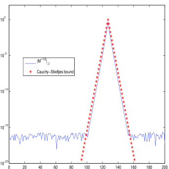
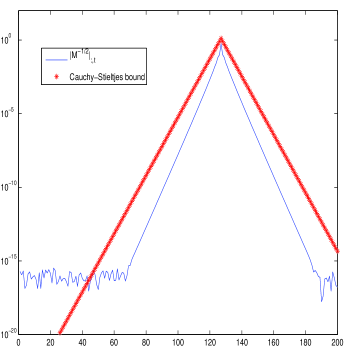
Fig. 4: Estimates for $|M^{-1/2}|_{:,t}$, $t=127$, using (12), size $n=200$, Log-scale. Left: $M={\rm tridiag}(-1,4,-1)$. Right: $M={\rm pentadiag}(-0.5,-1,4,-1,-0.5)$.

We conclude this section with a discussion on decay bounds for functions of $M-i\zeta I$, where $\zeta\in{\mathbb{R}}$. These estimates may be useful when the integral is over a complex curve. We first recall a result of Freund for $(M-i\zeta I)^{-1}$. To this end, we let again $\lambda_{\min},\lambda_{\max}$ be the extreme eigenvalues of $M$ (assumed to be HPD), and we let $\lambda_{1}=\lambda_{\min}-i\zeta$, $\lambda_{2}=\lambda_{\max}-i\zeta$.

Proposition 10.

Assume $M$ is Hermitian positive definite and $\beta$-banded. Let $R>1$ be defined as $R=\alpha+\sqrt{\alpha^{2}-1}$, with $\alpha=(|\lambda_{1}|+|\lambda_{2}|)/|\lambda_{2}-\lambda_{1}|$. Then for $k\neq t$,

$$|(M-i\zeta I)^{-1}|_{tk}\leq C(\zeta)\left(\frac{1}{R}\right)^{\frac{|t-k|}{\beta}}\,\,{\rm with}\,\,C(\zeta)=\frac{2R}{|\lambda_{1}-\lambda_{2}|}\frac{4R^{2}}{(R^{2}-1)^{2}}.$$

With this bound, we can modify (11) so as to handle more general matrices as follows. Once again, we let $\lambda_{\min},\lambda_{\max}$ be the extreme eigenvalues of $M$, and now we let $\lambda_{1}=\lambda_{\min}-i\zeta-\omega$, $\lambda_{2}=\lambda_{\max}-i\zeta-\omega$; $\alpha$ and $R$ are defined accordingly.

$$|f(M-i\zeta I)|_{kt}\leq\int_{-\infty}^{0}C\left(\frac{1}{R}\right)^{\frac{|k-t|}{\beta}}{\rm d}\gamma(\omega),\quad k\neq t.\quad$$ (15)

Since $R=R(\zeta,\omega)$ is defined in terms of spectral information of the shifted matrix $M-i\zeta I-\omega I$, we also obtain $C=C(\zeta,\omega)=\frac{2R(\zeta,\omega)}{|\lambda_{\max}-\lambda_{\min}|}\frac{4R(\zeta,\omega)^{2}}{(R(\zeta,\omega)^{2}-1)^{2}}$.

5 Extensions to more general sparse matrices

Although all our main results so far have been stated for matrices that are banded, it is possible to extend the previous bounds to functions of matrices with general sparsity patterns.

Following the approach in [14] and [7], let $G=(V,E)$ be the undirected graph describing the nonzero pattern of $M$. Here $V$ is a set of $n$ vertices (one for each row/column of $M$) and $E$ is a set of edges. The set $E\subseteq V\times V$ is defined as follows: there is an edge $(i,j)\in E$ if and only if $M_{ij}\neq 0$ (equivalently, $M_{ji}\neq 0$ since $M=M^{*}$). Given any two nodes $i$ and $j$ in $V$, a path of length $k$ between $i$ and $j$ is a sequence of nodes $i_{0}=i,i_{1},i_{2},\ldots,i_{k-1},i_{k}=j$ such that $(i_{\ell},i_{\ell+1})\in E$ for all $\ell=0,1,\ldots,k-1$ and $i_{\ell}\neq i_{m}$ for $\ell\neq m$. If $G$ is connected (equivalently, if $M$ is irreducible, which we will assume to be the case), then there exists a path between any two nodes $i,j\in V$. The geodesic distance $d(i,j)$ between two nodes $i,j\in G$ is then the length of the shortest path joining $i$ and $j$. With this distance, $(G,d)$ is a metric space.

We can then extend every one of the bounds seen so far for banded $M$ to a general sparse matrix $M=M^{*}$ simply by systematically replacing the quantity $\frac{|k-t|}{\beta}$ by the geodesic distance $d(k,t)$. Hence, the decay in the entries of $f(M)$ is to be understood in terms of distance from the nonzero pattern of $M$, rather than away from the main diagonal. We refer again to [7] for details. We note that this extension easily carries over to the bounds presented in the following section.

Finally, we observe that all the results in this paper apply to the case where $M$ is an infinite matrix with bounded spectrum, provided that $f$ has no singularities on an open neighborhood of the spectral interval $[\lambda_{\min},\lambda_{\max}]$. This implies that our bounds apply to all the $n\times n$ principal submatrices (“finite sections”) of such matrices, and that the bounds are uniform in $n$ as $n\to\infty$.

6 Estimates for functions of Kronecker sums of matrices

The decay pattern for matrices with Kronecker structure has a rich structure. In addition to a decay away from the diagonal, which depends on the matrix bandwidth, a “local” decay can be observed within the bandwidth; see Figure 5. This particular pattern was described for $f(x)=x^{-1}$ in [11]; here we largely expand on the class of functions for which the phenomenon can be described.

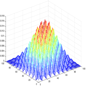
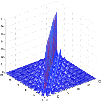
Fig. 5: Three-dimensional decay plots for $[f({\cal A})]_{ij}$ where $\cal A$ is the 5-point finite difference discretization of the negative Laplacian on the unit square on a $10\times 10$ uniform grid with zero Dirichlet boundary conditions. Left: $f({\cal A})=\exp(-5{\cal A})$. Right: $f({\cal A})={\cal A}^{-1/2}$.

Some matrix functions enjoy properties that make their application to Kronecker sums of matrices particularly simple. This is the case for instance of the exponential and certain trigonometric functions like $\sin(x)$ and $\cos(x)$. For these, bounds for their entries can be directly obtained from the estimates of the previous sections.

6.1 The exponential function

Recall the relation (2), which implies that

$$\exp(-\tau{\cal A})=\exp(-\tau M)\otimes\exp(-\tau M),\quad\tau\in{\mathbb{R}}$$ (16)

when ${\cal A}=M\otimes I+I\otimes M$. Here and in the following, a lexicographic ordering of the entries will be used, so that each row or column index $k$ of ${\cal A}$ corresponds to the pair $k=(k_{1},k_{2})$ in the two-dimensional Cartesian grid. Furthermore, for any fixed values of $\tau,\rho,\beta>0$, define

$$\Phi(i,j):=\left\{\begin{array}[]{ll}10\exp\left(-\frac{(|i-j|/\beta)^{2}}{5\rho\tau}\right),&\textnormal{for}\quad\sqrt{4\rho\tau}\leq\frac{|i-j|}{\beta}\leq 2\rho\tau,\\ 10\frac{\exp(-\rho\tau)}{\rho\tau}\left(\frac{{\rm e}\rho\tau}{\frac{|i-j|}{\beta}}\right)^{\frac{|i-j|}{\beta}},&\textnormal{for}\quad\frac{|i-j|}{\beta}\geq 2\rho\tau.\end{array}\right.$$ (17)

Note that $\Phi(i,j)$ is only defined for $|i-j|>\sqrt{4\rho\tau}\beta$. With these notations, the following bounds can be obtained.

Theorem 11.

Let $M$ be Hermitian and positive semidefinite with bandwidth $\beta$ and spectrum contained in $[0,4\rho]$, and let ${\cal A}=I\otimes M+M\otimes I$. Then

$$(\exp(-\tau{\cal A}))_{kt}=(\exp(-\tau M))_{k_{1}t_{1}}(\exp(-\tau M))_{k_{2}t_{2}}.$$

Therefore, for $\tau>0$

$$|(\exp(-\tau{\cal A}))_{kt}|\leq\Phi(k_{1},t_{1})\Phi(k_{2},t_{2})$$

for all $t=(t_{1},t_{2})$ and $k=(k_{1},k_{2})$ with $\min\{|t_{1}-k_{1}|,|t_{2}-k_{2}|\}\geq\sqrt{4\rho\tau}\beta$.

Proof.

Using (2) we obtain

$$e_{k}^{T}\exp(-{\tau\cal A})e_{t}=e_{k}^{T}\exp(-\tau M)\otimes\exp(-\tau M)e_{t}.$$

Let $E_{t_{1}t_{2}}$ be the $n\times n$ matrix such that $e_{t}={\rm vec}(E_{t_{1}t_{2}})\in{\mathbb{R}}^{n^{2}}$, and in particular $E_{t_{1}t_{2}}=e_{t_{1}}e_{t_{2}}^{T}$, with $e_{t_{1}},e_{t_{2}}\in{\mathbb{R}}^{n}$. Then

$$e_{k}^{T}\exp(-\tau M)\otimes\exp(-\tau M)e_{t} = e_{k}^{T}{\rm vec}(\exp(-\tau M)E_{t_{1}t_{2}}\exp(-\tau M)^{*})$$

$$= e_{k}^{T}{\rm vec}(\exp(-\tau M)e_{t_{1}}e_{t_{2}}^{T}\exp(-\tau M)^{*})$$

$$= e_{k}^{T}\begin{bmatrix}\exp(-\tau M)e_{t_{1}}(e_{t_{2}}^{T}\exp(-\tau M)^{*})e_{1}\\ \exp(-\tau M)e_{t_{1}}(e_{t_{2}}^{T}\exp(-\tau M)^{*})e_{2}\\ \vdots\\ \exp(-\tau M)e_{t_{1}}(e_{t_{2}}^{T}\exp(-\tau M)^{*})e_{n}\end{bmatrix}$$

$$= e_{k_{1}}^{T}\exp(-\tau M)e_{t_{1}}(e_{t_{2}}^{T}\exp(-\tau M)^{*})e_{k_{2}}),$$

which proves the first relation for $M$ Hermitian. For the bound, it is sufficient to use (17) to obtain the desired conclusion. ∎

The result can be easily generalized to a broader class of matrices.

Corollary 12.

Let ${\cal A}=I\otimes M_{1}+M_{2}\otimes I$ with $M_{1}$ and $M_{2}$ having bandwidth $\beta_{1}$ and $\beta_{2}$, respectively. Also, let the spectrum of $M_{1}$ be contained in the interval $[0,4\rho_{1}]$ and that of $M_{2}$ in the interval $[0,4\rho_{2}]$, with $\rho_{1},\rho_{2}>0$. Then for $t=(t_{1},t_{2})$ and $k=(k_{1},k_{2})$, with $|t_{\ell}-k_{\ell}|\geq\sqrt{4\rho_{\ell}\tau}\beta_{\ell}$, $\ell=1,2$,

$$(\exp(-\tau{\cal A}))_{kt}=(\exp(-\tau M_{1}))_{k_{1}t_{1}}(\exp(-\tau M_{2}))_{t_{2}k_{2}}.$$

Therefore,

$$|(\exp(-\tau{\cal A}))_{kt}|\leq\Phi_{1}(k_{1},t_{1})\Phi_{2}(k_{2},t_{2})$$

where $\Phi_{k}(i,j)$ is defined as $\Phi(i,j)$ in (17) with $\rho_{\ell}$, $\beta_{\ell}$ replacing $\rho$, $\beta$.

Generalization to the case of Kronecker sums of more than two matrices is relatively straightforward. Consider for example the case of three summands. A lexicographic order of the entries is again used, so that each row or column index $k$ of ${\cal A}=M\otimes I\otimes I+I\otimes M\otimes I+I\otimes I\otimes M$ corresponds to a triplet $k=(k_{1},k_{2},k_{3})$ in the three-dimensional Cartesian grid.

Corollary 13.

Let $M$ be $\beta$-banded, Hermitian and with spectrum contained in $[0,4\rho]$, and let ${\cal A}=M\otimes I\otimes I+I\otimes M\otimes I+I\otimes I\otimes M$ and $k=(k_{1},k_{2},k_{3})$ and $t=(t_{1},t_{2},t_{3})$. Then

$$(\exp(-\tau{\cal A}))_{kt}=(\exp(-\tau M))_{k_{1},t_{1}}(\exp(-\tau M))_{t_{2},k_{2}}(\exp(-\tau M))_{t_{3},k_{3}},$$

from which it follows

$$|(\exp(-\tau{\cal A}))_{kt}|\leq\Phi(k_{1},t_{1})\Phi(k_{2},t_{2})\Phi(k_{3},t_{3}),$$

for all $(k_{1},t_{1}),(k_{2},t_{2}),(k_{3},t_{3})$ with $\min\{|k_{1}-t_{1}|,|k_{2}-t_{2}|,|k_{3}-t_{3}|\}>\sqrt{4\tau\rho}\beta$.

Proof.

We write ${\cal A}=M\otimes(I\otimes I)+I\otimes(M\otimes I+I\otimes M)$, so that

$$\exp(-\tau{\cal A}) = \exp(-\tau M)\otimes\exp(-\tau M\otimes I+I\otimes(-\tau M))$$

$$= \exp(-\tau M)\otimes\exp(-\tau M)\otimes\exp(-\tau M).$$

Therefore, using $i=(t_{1},t_{2})$,

$$(\exp(-\tau{\cal A}))_{kt} = e_{k}^{T}{\rm vec}\left((\exp(-\tau M)\otimes\exp(-\tau M))e_{i}e_{t_{3}}^{T}\exp(-\tau M)\right)$$

$$= e_{k}^{T}{\rm vec}\left({\rm vec}(\exp(-\tau M)e_{t_{1}}e_{t_{2}}^{T}\exp(-\tau M))e_{t_{3}}^{T}\exp(-\tau M)\right)$$

$$= e_{k}^{T}{\rm vec}\left(\begin{bmatrix}\exp(-\tau M)e_{t_{1}}(e_{t_{2}}^{T}\exp(-\tau M)e_{1})\\ \exp(-\tau M)e_{t_{1}}(e_{t_{2}}^{T}\exp(-\tau M)e_{2})\\ \vdots\\ \exp(-\tau M)e_{t_{1}}(e_{t_{2}}^{T}\exp(-\tau M)e_{n})\end{bmatrix}\right)e_{t_{3}}^{T}\exp(-\tau M)$$

$$= (e_{k_{1}}^{T}\exp(-\tau M)e_{t_{1}})\,(e_{t_{2}}^{T}\exp(-\tau M)e_{k_{2}})\,(e_{t_{3}}^{T}\exp(-\tau M)e_{k_{3}}).$$

The rest follows as in the proof of Theorem 11. ∎

Remark 14.

Using (3), one can obtain similar bounds for $\cos({\cal A})$ and $\sin({\cal A})$, where ${\cal A}=M_{1}\otimes I+I\otimes M_{2}$ with $M_{1}$, $M_{2}$ banded.

6.2 Laplace–Stieltjes functions

If $f$ is a Laplace–Stieltjes function, then $f({\cal A})$ is well-defined and exploiting the relation (2) we can write

$$f({\cal A})=\int_{0}^{\infty}\exp(-\tau{\cal A}){\rm d}\alpha(\tau)=\int_{0}^{\infty}\exp(-\tau M)\otimes\exp(-\tau M){\rm d}\alpha(\tau).$$

Thus, using $k=(k_{1},k_{2})$ and $t=(t_{1},t_{2})$,

$$(f({\cal A}))_{kt} = \int_{0}^{\infty}e_{k}^{T}\exp(-\tau M)\otimes\exp(-\tau M)e_{t}{\rm d}\alpha(\tau)$$

$$= \int_{0}^{\infty}(\exp(-\tau M))_{k_{1}t_{1}}(\exp(-\tau M))_{t_{2}k_{2}}{\rm d}\alpha(\tau).$$

With the notation of Theorem 7, we have

$$|f({\cal A})|_{kt}\leq\int_{0}^{\infty}\exp(-2\lambda_{\min}\tau)|\exp(-\tau\widehat{M})|_{k_{1}t_{1}}|\exp(-\tau\widehat{M})|_{k_{2}t_{2}}{\rm d}\alpha(\tau).$$ (18)

In this form, the bound (18), of course, is not particularly useful. Explicit bounds can be obtained, for specific examples of Laplace–Stieltjes functions, by evaluating or bounding the integral on the right-hand side of (18).

For instance, using once again the inverse square root, so that $\alpha(\tau)=\sqrt{\pi/\tau}$, we obtain

$$|{\cal A}^{-\frac{1}{2}}|_{kt} \leq \sqrt{\pi}\int_{0}^{\infty}\frac{1}{\sqrt{\tau^{3}}}\exp(-2\lambda_{\min}\tau)|\exp(-\tau\widehat{M})|_{k_{1}t_{1}}|\exp(-\tau\widehat{M})|_{k_{2}t_{2}}{\rm d}\tau$$

$$\leq \sqrt{\pi}\left(\int_{0}^{\infty}\left(\frac{1}{\tau^{3/4}}\exp(-\lambda_{\min}\tau)|\exp(-\tau\widehat{M})|_{k_{1}t_{1}}\right)^{2}{\rm d}\tau\right)^{\frac{1}{2}}\cdot$$

$$\qquad\left(\int_{0}^{\infty}\left(\frac{1}{\tau^{3/4}}\exp(-\lambda_{\min}\tau)|\exp(-\tau\widehat{M})|_{k_{2}t_{2}}\right)^{2}{\rm d}\tau\right)^{\frac{1}{2}}.$$

The two integrals can then be bounded as done in Theorem 7. For the other example we have considered earlier, namely the function $f(x)=(1-\exp(-x))/x$, the bound is the same except that $\sqrt{\pi}/\sqrt{\tau^{3}}$ is replaced by one, and the integration interval reduces to $[0,1]$; see also Example 15 next.

Example 15.

We consider again the function $f(x)=(1-\exp(-x))/x$, and the two choices of matrix $M$ in Example 6; for each of them we build $\cal A$ as the Kronecker sum ${\cal A}=M\otimes I+I\otimes M$. The entries of the $t$th column with $t=94$, that is $(t_{1},t_{2})=(14,5)$ are shown in Figure 6, together with the bound obtained above. The oscillating pattern is well captured in both cases, with a particularly good accuracy also in terms of magnitude in the tridiagonal case. The lack of approximation near the diagonal reflects the condition $|k_{i}-t_{i}|/\beta\geq 2$, $i=1,2$.

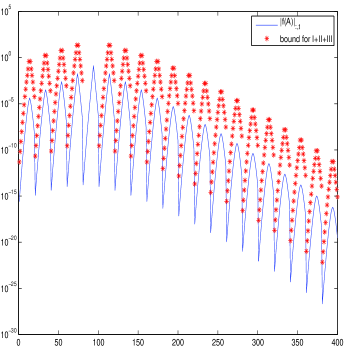
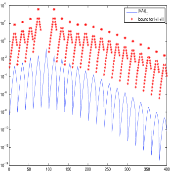
Fig. 6: Example 15. True decay and estimates for $|f(A)|_{:,t}$, $t=94$, $A=M\otimes I+I\otimes M$ of size $n=400$. Left: $M={\rm tridiag}(-1,4,-1)$. Right: $M={\rm pentadiag}(-0.5,-1,4,-1,-0.5)$.

Remark 16.

These results can be easily extended to the case where ${\cal A}=M_{1}\otimes I+I\otimes M_{2}$ with $M_{1}$, $M_{2}$ both Hermitian positive definite and having bandwidths $\beta_{1}$, $\beta_{2}$. It can also be generalized to the case where ${\cal A}$ is the Kronecker sum of three or more banded matrices.

6.3 Cauchy–Stieltjes functions

If $f$ is a Cauchy–Stieltjes function and $\cal A$ has no eigenvalues on the closed set $\Gamma\subset{\mathbb{C}}$, then

$$f({\cal A})=\int_{\Gamma}({\cal A}-\omega I)^{-1}{\rm d}\gamma(\omega),$$

so that

$$e_{k}^{T}f({\cal A})e_{t}=\int_{\Gamma}e_{k}^{T}({\cal A}-\omega I)^{-1}e_{t}{\rm d}\gamma(\omega).$$

We can write ${\cal A}-\omega I=M\otimes I+I\otimes(M-\omega I)$. Each column $t$ of the matrix inverse, $x_{t}:=(\omega I-{\cal A})^{-1}e_{t}$, may be viewed as the matrix solution $X_{t}=X_{t}(\omega)\in{\mathbb{C}}^{n\times n}$ to the following Sylvester matrix equation:

$$MX_{t}+X_{t}(M-\omega I)=E_{t},\qquad x_{t}={\rm vec}(X_{t}),\quad e_{t}={\rm vec}(E_{t}),$$

where the only nonzero element of $E_{t}$ is in position $(t_{1},t_{2})$; here the same lexicographic order of the previous sections is used to identify $t$ with $(t_{1},t_{2})$.

From now on, we assume that $\Gamma=(-\infty,0]$. We observe that the Sylvester equation has a unique solution, since no eigenvalue of $M$ can be an eigenvalue of $\omega I-M$ for $\omega\leq 0$ (recall that $M$ is Hermitian positive definite).

Following Lancaster ([35, p.556]), the solution matrix $X_{t}$ can be written as

$$X_{t}=-\int_{0}^{\infty}\exp(-\tau M)E_{t}\exp(-\tau(M-\omega I)){\rm d}\tau.$$

For $k=(k_{1},k_{2})$ and $t=(t_{1},t_{2})$ this gives

$$e_{k}^{T}(\omega I-{\cal A})^{-1}e_{t} = e_{k_{1}}^{T}X_{t}e_{k_{2}}$$ (20)

$$= -\int_{0}^{\infty}e_{k_{1}}^{T}\exp(-\tau M)e_{t_{1}}e_{t_{2}}^{T}\exp(-\tau(M-\omega I))e_{k_{2}}{\rm d}\tau.$$

Therefore, in terms of the original matrix function component,

$$e_{k}^{T}f({\cal A})e_{t}=-\int_{-\infty}^{0}\int_{0}^{\infty}e_{k_{1}}^{T}\exp(-\tau M)e_{t_{1}}e_{t_{2}}^{T}\exp(-\tau(M-\omega I))e_{k_{2}}{\rm d}\tau{\rm d}\gamma(\omega).$$

We can thus bound each entry as

$$|e_{k}^{T}f({\cal A})e_{t}|\leq\int_{0}^{\infty}\left(|\exp(-\tau M)|_{k_{1}t_{1}}|\exp(-\tau M)|_{k_{2}t_{2}}\int_{-\infty}^{0}\exp(\tau\omega){\rm d}\gamma(\omega)\right){\rm d}\tau.$$

It is thus apparent that $|e_{k}^{T}f({\cal A})e_{t}|$ can be bounded in a way analogous to the case of Laplace–Stieltjes functions, once the term $\int_{-\infty}^{0}\exp(\tau\omega){\rm d}\gamma(\omega)$ is completely determined. In particular, for $f(x)=x^{-1/2}$, we obtain

$$\int_{-\infty}^{0}\exp(\tau\omega){\rm d}\gamma(\omega) = \frac{1}{\pi}\int_{-\infty}^{0}\exp(\tau\omega)\frac{1}{\sqrt{-\omega}}{\rm d}\omega$$

$$= \frac{2}{\pi}\int_{0}^{\infty}\exp(-\tau\eta^{2})\frac{1}{\eta}{\rm d}\eta$$

$$= \frac{2}{\pi}\frac{\sqrt{\pi}}{2\sqrt{\tau}}=\frac{1}{\sqrt{\pi}}f(\tau).$$

Therefore,

$$\!\!|{\cal A}^{-\frac{1}{2}}|_{kt}\leq\frac{1}{\sqrt{\pi}}\!\!\left(\int_{0}^{\infty}\!\!\!|\exp(-\tau M)|_{k_{1}t_{1}}^{2}f(\tau)d\tau)\!\right)^{\frac{1}{2}}\!\!\left(\int_{0}^{\infty}\!\!\!|\exp(-\tau M)|_{k_{2}t_{2}}^{2}f(\tau)d\tau)\!\right)^{\frac{1}{2}}.$$ (21)

Using once again the bounds in Theorem 5 a final integral upper bound can be obtained, in the same spirit as for Laplace–Stieltjes functions.

We explicitly mention that the solution matrix $X_{t}$ could be alternatively written in terms of the resolvent $(M-\zeta iI)^{-1}$, with $\zeta\in{\mathbb{R}}$ [35]. This would allow us to obtain an integral upper bound for $|e_{k}^{T}f({\cal A})e_{t}|$ by means of Proposition 10 and of (15). We omit the quite technical computations, however the final results are qualitatively similar to those obtained above.

Example 17.

In Figure 7 we report the actual decay and our estimate following (21) for the inverse square root, again using the two matrices of our previous examples. We observe that having used estimates for the exponential to handle the Kronecker form, the approximations are slightly less sharp than previously seen for Cauchy–Stieltjes functions. Nonetheless, the qualitative behavior is captured in both instances.

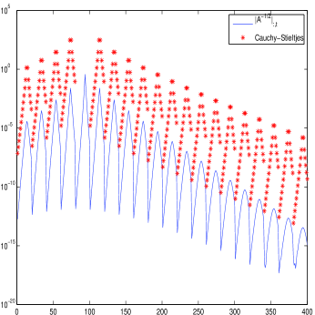
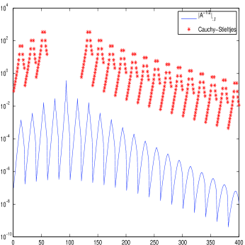
Fig. 7: Example 17. True decay and estimates for $|A^{-\frac{1}{2}}|_{:,t}$, $t=94$, $A=M\otimes I+I\otimes M$ of size $n=400$. Left: $M={\rm tridiag}(-1,4,-1)$. Right: $M={\rm pentadiag}(-0.5,-1,4,-1,-0.5)$.

Remark 18.

As before, the estimate for $(f({\cal A}))_{k,t}$ can be generalized to the sum ${\cal A}=M_{1}\otimes I+I\otimes M_{2}$, with both $M_{1},M_{2}$ Hermitian and positive definite matrices.

Remark 19.

Using the previous remark, the estimate for the matrix function entries can be generalized to matrices that are sums of several Kronecker products. For instance, if

$${\cal A}=M\otimes I\otimes I+I\otimes M\otimes I+I\otimes I\otimes M,$$

then we can write

$${\cal A}=M\otimes(I\otimes I)+I\otimes(M\otimes I+I\otimes M)=:M\otimes I+I\otimes M_{2},$$

so that, following the same lines as in (20) we get

$$e_{k}^{T}f({\cal A})e_{t} = \int_{\Gamma}e_{k}^{T}({\cal A}-\omega I)^{-1}e_{t}{\rm d}\gamma(\omega)$$

$$= -\int_{\Gamma}\int_{0}^{\infty}e_{k_{1}}^{T}\exp(-\tau M)^{-1}e_{t_{1}}e_{t_{2}}^{T}\exp(-\tau(M_{2}-\omega I))e_{k_{2}}{\rm d}\tau{\rm d}\gamma(\omega).$$

Since $M_{2}=M\otimes I+I\otimes M$, we then obtain $e_{t_{2}}^{T}\exp(-\tau M_{2})e_{k_{2}}=e_{t_{2}}^{T}\exp(-\tau M)\otimes\exp(-\tau M)e_{k_{2}}$. Splitting $t_{2},k_{2}$ in their one-dimensional indices, the available bounds can be employed to obtain a final integral estimate.

7 Conclusions

In this paper we have obtained new decay bounds for the entries of certain analytic functions of banded and sparse matrices, and used these results to obtain bounds for functions of matrices that are Kronecker sums of banded (or sparse) matrices. The results apply to strictly completely monotonic functions and to Markov functions, which include a wide variety of functions arising in mathematical physics, numerical analysis, network science, and so forth.

The new bounds are in many cases considerably sharper than previously published bounds and they are able to capture the oscillatory, non-monotonic decay behavior observed in the entries of $f({\cal A})$ when $\cal A$ is a Kronecker sum. Also, the bounds capture the superexponential decay behavior observed in the case of entire functions.

A major difference with previous decay results is that the new bounds are given in integral form, therefore their use requires some work on the part of the user. If desired, these quantities can be further bounded for specific function choices. In practice, the integrals can be evaluated numerically to obtain explicit bounds on the quantities of interest.

Although in this paper we have focused mostly on the Hermitian case, extensions to functions of more general matrices may be possible, as long as good estimates on the entries of the matrix exponential and resolvent are available. We leave the development of this idea for possible future work.

References

- [1] E. Aune, D. P. Simpson, and J. Eidsvik, Parameter estimation in high dimensional Gaussian distributions, Stat. Comput., 24 (2014), pp. 247–263.
- [2] A. G. Baskakov, Wiener’s theorem and the asymptotic estimates of the elements of inverse matrices, Funct. Anal. Appl., 24 (1990), pp. 222–224.
- [3] A. G. Baskakov, Estimates for the entries of inverse matrices and the spectral analysis of linear operators, Izvestiya: Mathematics, 61 (1997), pp. 1113–1135.
- [4] M. Benzi and P. Boito, Decay properties for functions of matrices over -algebras, Linear Algebra Appl., 456 (2014), pp. 174–198.
- [5] M. Benzi, P. Boito and N. Razouk, Decay properties of spectral projectors with applications to electronic structure, SIAM Rev., 55 (2013), pp. 3–64.
- [6] M. Benzi and G. H. Golub, Bounds for the entries of matrix functions with applications to preconditioning, BIT Numer. Math., 39 (1999), pp. 417–438.
- [7] M. Benzi and N. Razouk, Decay bounds and algorithms for approximating functions of sparse matrices, Electr. Trans. Numer. Anal., 28 (2007), pp. 16–39.
- [8] S. Bernstein, Sur les fonctions absolument monotones, Acta Math., 52 (1929), pp. 1–66.
- [9] D. A. Bini, G. Latouche, and B. Meini, Numerical Methods for Structured Markov Chains, Oxford University Press, Oxford, UK, 2005.
- [10] D. R. Bowler and T. Miyazaki, methods in electronic structure calculations, Rep. Progr. Phys., 75:036503, 2012.
- [11] C. Canuto, V. Simoncini, and M. Verani, On the decay of the inverse of matrices that are sum of Kronecker products, Linear Algebra Appl., 452 (2014), pp. 21–39.
- [12] C. Canuto, V. Simoncini, and M. Verani, Contraction and optimality properties of an adaptive Legendre–Galerkin method: the multi-dimensional case, J. Sci. Comput., DOI:10.1007/s109150014-9912-3, July 2014.
- [13] M. Cramer and J. Eisert, Correlations, spectral gap and entanglement in harmonic quantum systems on generic lattices, New J. Phys., 8 (2006), 71.
- [14] M. Cramer, J. Eisert, M. B. Plenio and J. Dreissig, Entanglement-area law for general bosonic harmonic lattice systems, Phys. Rev. A, 73 (2006), 012309.
- [15] N. Del Buono, L. Lopez and R. Peluso, Computation of the exponential of large sparse skew-symmetric matrices, SIAM J. Sci. Comput., 27 (2005), pp. 278–293.
- [16] S. Demko, Inverses of band matrices and local convergence of spline projections, SIAM J. Numer. Anal., 14 (1977), pp. 616–619.
- [17] S. Demko, W. F. Moss, and P. W. Smith, Decay rates for inverses of band matrices, Math. Comp., 43 (1984), pp. 491–499.
- [18] V. Druskin and L. Knizhnerman, Krylov subspace approximation of eigenpairs and matrix functions in exact and computer arithmetic, Numer. Linear Algebra Appl., 2(3), (1995), pp. 205–217.
- [19] V. Druskin and L. Knizhnerman, Two polynomial methods of calculating functions of symmetric matrices, U.S.S.R. Comput. Math. Math. Phys., 29, (1989), pp. 112–121 (Pergamon Press, translation from Russian).
- [20] J. Dubordieu, Sur un théorème de M. Bernstein relatif à la transformation de Laplace–Stieltjes, Compositio Math., 7 (1940), pp. 96–111.
- [21] V. Eijkhout and B. Polman, Decay rates of inverses of banded -matrices that are near to Toeplitz matrices, Linear Algebra Appl., 109 (1988), pp. 247–277.
- [22] J. Eisert, M. Cramer and M. B. Plenio, Colloquium: Area laws for the entanglement entropy, Rev. Modern Phys., 82 (2010), pp. 277–306.
- [23] R. Freund, On polynomial approximations to with complex and some applications to certain non-Hermitian matrices, Approx. Theory Appl., 5 (1989), pp. 15–31.
- [24] P.-L. Giscard, K. Lui, S. J. Thwaite, and D. Jaksch, An Exact Formulation of the Time-Ordered Exponential Using Path-Sums, arXiv:1410.6637v1 [math-ph], 24 October 2014.
- [25] K. Gröchenig and A. Klotz, Noncommutative approximation: inverse-closed subalgebras and off-diagonal decay of matrices, Constr. Approx., 32 (2010), pp. 429–466.
- [26] K. Gröchenig and M. Leinert, Symmetry and inverse-closedness of matrix algebras and functional calculus for infinite matrices, Trans. Amer. Math. Soc., 358 (2006), pp. 2695–2711.
- [27] S. Güttel and L. Knizhnerman, A black-box rational Arnoldi variant for Cauchy–Stieltjes matrix functions, BIT Numer. Math., 53 (2013), pp. 595–616.
- [28] A. Haber and M. Verhaegen, Sparse Solution of the Lyapunov Equation for Large-Scale Interconnected Systems, arXiv:1408:3898 [math.OC], 18 August 2014.
- [29] N. J. Higham, Matrix Functions – Theory and Applications, SIAM, Philadelphia, USA, 2008.
- [30] M. Hochbruck and J. J. Lubich, On Krylov subspace approximations to the matrix exponential operator, SIAM J. Numer. Anal., 34 (1997), pp. 1911–1925.
- [31] A. Iserles, How large is the exponential of a banded matrix?, New Zealand J. Math., 29 (2000), pp. 177–192.
- [32] S. Jaffard, Propriétés des matrices “bien localisées” près de leur diagonale et quelques applications, Ann. Inst. Henri Poincarè, 7 (1990), pp. 461–476.
- [33] D. Kershaw, Inequalities on the elements of the inverse of a certain tri-diagonal matrix, Math. Comp., 24 (1970), pp. 155–158.
- [34] I. Kryshtal, T. Strohmer and T. Wertz, Localization of matrix factorizations, Found. Comput. Math., DOI 10.1007/s10208-014-9196-x
- [35] P. Lancaster, Explicit solutions of linear matrix equations, SIAM Rev., 12 (1970), pp. 544–566.
- [36] L. Lin, Localized Spectrum Slicing, arXiv:1411.6152v1 [math.NA] 22 November 2014.
- [37] N. Mastronardi, M. K. Ng, and E. E. Tyrtyshnikov, Decay in functions of multi-band matrices, SIAM J. Matrix Anal. Appl., 31 (2010), pp. 2721–2737.
- [38] N. Merkle, Completely monotone functions — a digest, arXiv:1211.0900v1 [math.CA] 2 November 2012.
- [39] G. Meurant, A review of the inverse of symmetric tridiagonal and block tridiagonal matrices, SIAM J. Matrix Anal. Appl., 13 (1992), pp. 707–728.
- [40] L. Molinari, Identities and exponential bounds for transfer matrices, J. Phys. A: Math. and Theor., 46 (2013), 254004.
- [41] M. Shao, On the finite section method for computing exponentials of doubly-infinite skew-Hermitian matrices, Linear Algebra Appl., 451 (2014), pp. 65–96.
- [42] T. Strohmer, Four short stories about Toeplitz matrix calculations, Linear Algebra Appl.,343-344 (2002), pp. 321–344.
- [43] R. S. Varga, Nonnegatively posed problems and completely monotonic functions, Lin. Algebra Appl., 1 (1968), pp. 329–347.
- [44] D. V. Widder, The Laplace Transform, Princeton University Press, 1946.
- [45] Q. Ye, Error bounds for the Lanczos method for approximating matrix exponentials, SIAM J. Numer. Anal., 51 (2013), pp. 68–87.