ALMA Multi-line Observations of the IR-bright Merger VV 114

Abstract

We present ALMA cycle 0 observations of the molecular gas and dust in the IR-bright mid-stage merger VV 114 obtained at 160 – 800 pc resolution. The main aim of this study is to investigate the distribution and kinematics of the cold/warm gas and to quantify the spatial variation of the excitation conditions across the two merging disks. The data contain 10 molecular lines, including the first detection of extranuclear CH₃OH emission in interacting galaxies, as well as continuum emission. We map the ¹²CO (3–2)/¹²CO (1–0) and the ¹²CO (1–0)/¹³CO (1–0) line ratio at 800 pc resolution (in the units of K km s^-1), and find that these ratios vary from 0.2 – 0.8 and 5 – 50, respectively. Conversely, the 200 pc resolution HCN (4–3)/HCO⁺ (4–3) line ratio shows low values ($<$ 0.5) at a filament across the disks except for the unresolved eastern nucleus which is three times higher (1.34 $\pm$ 0.09). We conclude from our observations and a radiative transfer analysis that the molecular gas in the VV 114 system consists of five components with different physical and chemical conditions; i.e., 1) dust-enshrouded nuclear starbursts and/or AGN, 2) wide-spread star forming dense gas, 3) merger-induced shocked gas, 4) quiescent tenuous gas arms without star formation, 5) H₂ gas mass of (3.8 $\pm$ 0.7) $\times$ 10⁷ M_⊙ (assuming a conversion factor of $\alpha_{\rm{CO}}$ = $0.8~{}\rm{M}_{\odot}~{}\rm{(K~{}km~{}s^{-1}~{}pc^{2})^{-1}}$) at the tip of the southern tidal arm, as a potential site of tidal dwarf galaxy formation.

1. INTRODUCTION

Galaxy interactions and mergers play important roles in triggering star formation and/or fueling the nuclear activity in the merging host galaxies (Hopkins et al., 2006). Recent high resolution simulations of major mergers show that large scale tidal forces as well as small scale turbulence and stellar feedback can significantly influence the distribution of gas, forming massive clumps of dense gas with $M_{\rm{H_{2}}}$ = 10⁶ – 10⁸ M_⊙ (e.g., Teyssier et al., 2010; Hopkins et al., 2013). These simulations also predict that the star formation not only increases as the galaxies first collide, but it also persists at a higher rate throughout the merger process, peaking at the final coalescence.

(Ultra-)Luminous Infrared Galaxies (U/LIRGs; Soifer et al., 1987) at low redshifts are almost exclusively strongly interacting and merging systems (Kartaltepe et al., 2010), often found at the mid to final stages of the merger. The elevated level of infrared luminosity originates from the reprocessed emission from the dust particles surrounding the starburst or the Active Galactic Nuclei (AGNs), both of which are likely triggered by the tidal interaction. The highest gas surface densities ($\Sigma_{\rm{H_{2}}}$ = 5.4 $\times$ 10⁴ – 1.4 $\times$ 10⁵ M_⊙ pc^-2) and consequently the highest star formation activities ($\Sigma_{\rm{SFR}}$ = $\sim$ 1000 M_⊙ yr^-1 kpc^-2) are usually found near the compact nuclear region (e.g., Arp220, NGC 6240; Downes & Solomon, 1998; Engel et al., 2010; Wilson et al., 2014). Dense molecular gas ($n$ $\sim$ 10⁵ – 10⁷ cm^-3) in U/LIRGs directly shows nuclear gas distribution and kinematics (e.g., Iono et al., 2004; Sakamoto et al., 2014). They are often surrounded by diffuse gas ($n$ $\sim$ 10² – 10³ cm^-3) that may or may not be directly associated with star formation activities.

It has been demonstrated that the HCN (4–3) and HCO⁺ (4–3) emission lines, whose critical densities are 8.5 $\times$ 10⁶ and 1.8 $\times$ 10⁶ cm^-3, respectively, can be used as tracers of the dense gas (e.g., Iono et al., 2013; Garcia-Burillo et al., 2014; Imanishi & Nakanishi, 2014). On the other hand, CO (1–0) and ¹³CO (1–0) line emission, whose critical densities are 4.1 $\times$ 10² and 1.5 $\times$ 10³ cm^-3, respectively, have been used extensively for tracing the global gas distribution and kinematics in merging U/LIRGs (e.g., Yun et al., 1994; Iono et al., 2004; Ueda et al., 2014). In addition, the ratio of these lines (e.g. ¹²CO/¹³CO and HCN/HCO⁺) have been used to investigate the properties of the ISM (Casoli et al., 1992; Aalto et al., 1997) or to search for buried AGNs (e.g., Imanishi et al., 2007; Imanishi & Nakanishi, 2014). Limitations in sensitivity and angular resolution have been the major obstacles in understanding the detailed distribution and kinematics of both dense and diffuse gas, and investigating the spatial variation of the line ratios and the physical condition of gas.

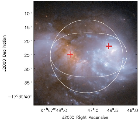
Figure 1.— The HST/ACS image of VV 114 (Evans, 2008). There is a dust lane from north to south in front of the eastern galaxy. The red crosses show the positions of the nuclei defined by the peak positions of the Ks-band observation (Tateuchi et al., 2012). The white ellipse shows a field of view of 3-point mosaic observation with band 7, while the white circle shows a field of view of 7-point mosaic observation with band 7 (see §2).

In this paper, we present Atacama Large Millimeter/submillimeter Array (ALMA) cycle 0 observations of the IR-bright merging galaxy VV 114. VV 114 is one of the best samples for studying the gas response during the critical stage when the two gas disks merge (Iono et al., 2005; Wilson et al., 2008). The target molecular lines include ¹²CO (1–0), ¹³CO (1–0), ¹²CO (3–2), HCN (4–3) and HCO⁺ (4–3), and we also present the maps of CH₃OH (2_k–1_k), CS (2–1), CN (1_1/2–0_1/2), CN (1_3/2–0_1/2), and CS (7–6) lines which were observed simultaneously within the same band. The main aim of this study is to investigate the distribution and kinematics of the diffuse and dense molecular gas and to quantify the spatial variation of the excitation conditions across the two merging disks.

VV 114 is a gas-rich ($M_{\rm{H_{2}}}$ = 5.1 $\times$ 10¹⁰ M_⊙; Yun et al., 1994) nearby (D = 82 Mpc; 1$\farcs$0 = 400 pc) interacting system (Figure 1) with high-infrared luminosity ($L_{\rm{IR}}$ = 4.7 $\times$ 10¹¹ $L_{\odot}$; Armus et al., 2009). The projected nuclear separation between the two optical galaxies (VV 114E and VV 114W) is about 6 kpc. Frayer et al. (1999) found a large amount of dust ($M_{\rm{dust}}$ = 1.2 $\times$ 10⁸ M_⊙) distributed across the system with a dust temperature of 20 – 25 K. About half of the warmer dust traced in the mid-IR (MIR) is associated with the eastern galaxy, where both compact (nuclear region) and extended emission is found (Le Floc’h et al., 2002). Rich et al. (2011) found a bimodal distribution of velocity dispersions of several atomic forbidden lines and emission line ratios indicative of composite activity explained by a combination of wide-spread shocks and star formation. The wide-spread star formation is also revealed by Pa$\alpha$ observation using ANIR camera mounted on miniTAO (Tateuchi et al., 2012, see also Appendix A.1). Iono et al. (2013) (hereafter paper I) identified a highly obscured AGN and compact starburst clumps using sub-arcsecond resolution ALMA cycle 0 observations of HCN (4–3) and HCO⁺ (4–3) emission.

This paper is organized as follows. We describe our observations and data reduction in §2, and results in §3. In §4 and §5, we provide molecular line ratios and physical parameters, such as the gas/dust mass, the gas temperature, and the gas density. In §6, we present the properties of “dense” gas (§6.1), the comparison between molecular gas and star formation (§6.2), the discussions of the CO isotope enhancement (§6.3), the gas-to-dust mass ratio (§6.4), the fractional abundances of CS, CH₃OH, and CN relative to H₂ (§6.5), and a potential tidal dwarf galaxy formations at the tip of the tidal arms of VV 114 (§6.6). We summarize and conclude this paper in §7. Throughout this paper, we adopt H₀ = 73 km s^-1 Mpc^-1, $\Omega_{\rm{M}}$ = 0.27, and $\Omega_{\rm{\Delta}}$ = 0.73.

2. OBSERVATIONS AND DATA REDUCTION

Observations toward VV 114 were carried out as an ALMA cycle 0 program (ID = 2011.0.00467.S; PI = D. Iono) using fourteen – twenty 12 m antennas. The band 3 and band 7 receivers were tuned to the ¹²CO (1–0), ¹³ CO (1–0), ¹²CO (3–2), HCN (4–3), and HCO⁺ (4–3) line emissions in the upper side band (see Table 1). The ¹²CO (1–0) data were obtained on November 6, 2011 and May 4, 2012 in the compact and extended configurations, respectively. The ¹³CO (1–0) data were obtained on May 27 and July 2, 2012 in the compact configuration. The ¹²CO (3–2) emission was observed on November 5, 2011 in the compact configuration (7-point mosaic). The HCN (4–3) and HCO⁺ (4–3) data were obtained on July 1, 2, and 3, 2012 in the extended configuration (3-point mosaic), simultaneously. Each spectral window had a bandwidth of 1.875 GHz with 3840 channels, and two spectral windows were set to each sideband to achieve a total frequency coverage of $\sim$ 7.5 GHz in these observations. The spectral resolution was 0.488 MHz per channel. J1924-292, J0132-169, Uranus (Neptune for band 3 observations) were used for bandpass, phase, and flux calibrations. Detailed observational parameters are shown in Table 1.

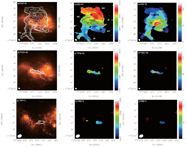
Figure 2.— (a) ¹²CO (1–0) integrated intensity image overlaid on the HST/ACS/F435W image of VV 114. The contours are 0.2, 0.4, 0.8, 1.6, 3.2, 6.4, 12.8, 25.6, and 33.0 Jy km s^-1. The dashed green box shows an imaging field of other lines and continuum of this work except for the CO and ¹³CO lines. (b) ¹²CO (1–0) velocity field image. The velocity field image in color scale ranges from 5600 km s^-1 to 6200 km s^-1. The dashed black lines represent tidal arms of VV 114. The dashed red line tracks the filamentary structure detected in images of other lines and dust continuum, and the dashed circle shows the overlap region. (c) ¹²CO (1–0) velocity dispersion image. The velocity dispersion image in color scale ranges from 0 km s^-1 to 120 km s^-1. (d) The same as (a) but for ¹³CO (1–0). The contours are 0.02, 0.04, 0.08, 0.16, 0.32, and 0.64 Jy km s^-1. (e/f) The same as (b/c), respectively, but for ¹³CO (1–0). (g) The same as (a) but for CS (2–1). The contours are 0.04, 0.08, 0.16, and 0.28 Jy km s^-1. (h/i) The same as (b/c), respectively, but for CS (2–1). The beam size of each line is shown in the bottom-left of the images (Table 2). The red crosses show the positions of the nuclei defined by the peak positions of the Ks-band observation (Tateuchi et al., 2012).

We used the delivered calibrated data and mapping was accomplished using the clean task in CASA (McMullin et al., 2007). We made the data cubes with a velocity width of 5 km s^-1 for the ¹²CO line and 30 km s^-1 for the other lines. All maps in this paper, except for ¹²CO (3–2), are reconstructed with a Briggs weighting (robust = 0.5; Briggs & Cornwell, 1992) and analyzed with MIRIAD and AIPS. The ¹²CO (3–2) images are created with uniform weighting (see §3.2). The synthesized beam size of the ¹²CO (1–0), ¹³CO (1–0), ¹²CO (3–2), and HCN (4–3) were 1$\farcs$97 $\times$ 1$\farcs$35 (P.A. = 82.3 deg.), 1$\farcs$77 $\times$ 1$\farcs$20 (P.A. = 85.8 deg.), 1$\farcs$64 $\times$ 1$\farcs$17 (P.A. = 112.6 deg.), and 0$\farcs$46 $\times$ 0$\farcs$38 (P.A. = 51.5 deg.), respectively. We also detected CN (1_3/2–0_1/2), CN (1_1/2–0_1/2), CS (2–1), CH₃OH (2_k-1_k), and CS (7–6) line emission for the first time in VV 114. The properties of these molecular lines are summarized in Table 2. All images which we constructed are corrected for primary beam attenuation. The on-source times of band 3 and band 7 were about 40 minutes and 80 minutes, and the rms noise levels of the channel maps with 30 km s^-1 resolution are 1.0 mJy beam^-1 and 0.8 mJy beam^-1, respectively. Furthermore, we made continuum maps at each observing frequency by adding the line-free channels. The rms level of the continuum images were 0.05 mJy beam^-1, 0.11 mJy beam^-1, and 0.07 mJy beam^-1 for band 3, band 7 in the compact configuration, and band 7 in the extended configuration, respectively. The continuum emission was subtracted in the $uv$-plane before making the line images. Throughout this paper, the pixel scales of the band 3 and the band 7 images are set to 0$\farcs$3/pixel and 0$\farcs$08/pixel, respectively, and only the statistical error is considered unless mentioned otherwise. The systematic error on the absolute flux is estimated to be $\sim$ 5% and $\sim$ 10% for both sidebands in band 3 and band 7, respectively.

In the following sections, we estimate the missing flux of each molecular line for which the single dish data are available in literature. Although the effect of missing flux becomes critical when we evaluate the global gas properties and the corresponding line ratios, the effect is negligible when we discuss structures that are smaller than the “maximum recoverable scale” (MRS) of each configuration of ALMA. This is estimated from the minimum baseline lengths of the assigned antenna configurations and the observed frequencies. The MRS of our observations are $\sim$ 8″ and $\sim$ 7″ in band 3 and band 7, respectively (Table 1). Therefore the missing flux effect in this paper is negligible, since we derive physical parameters (e.g., molecular gas mass) only for structures smaller than $\sim$ 2″.

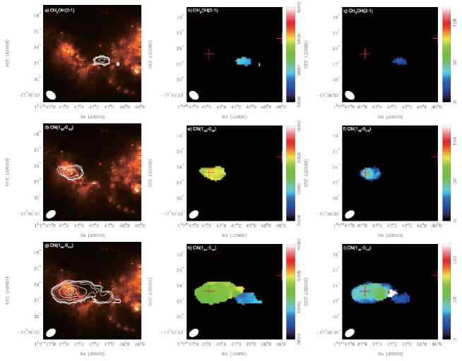
Figure 3.— The same as Figure 2 but for (a, b, and c) CH₃OH (2_k–1_k), (d, e, and f) CN (1_1/2–0_1/2), and (g, h, and i) CN (1_3/2–0_1/2). (a) The contours are 0.02, 0.04, 0.08, 0.16, and 0.32 Jy km s^-1 (d) The contours are 0.04, 0.08, 0.16, 0.32, and 0.50 Jy km s^-1. (g) The contours are 0.04, 0.08, 0.16, 0.32, 0.64, 1.00, and 1.20 Jy km s^-1.

3. RESULTS

Molecular line and continuum images are shown in Figures 2, 3, 4, 5, and 6. The channel maps and the spectra of all line emissions are shown in Appendix A.2 and A.3.

3.1. Line Emissions in Band 3

3.1.1 ¹²CO (1–0)

The integrated intensity, velocity field, and velocity dispersion maps of VV 114 are shown in Figures 2a, 2b, and 2c, respectively. The total ¹²CO (1–0) integrated intensity of VV 114 is 594.6 $\pm$ 1.6 Jy km s^-1, which is 1.3 times larger than that detected using the NRAO 12 m telescope (461 Jy km s^-1; Sanders et al., 1991). This is because the pointing center for the NRAO 12 m observation was 25$\farcs$0 southwest of the CO centroid identified from the ALMA map (NRAO 12 m: 01h07m45.7s, -17d30m36.5s; CO centroid: 01h07m47.2s, -17d30m25.8s). At the adopted distance of VV 114 (86 Mpc), the 1$\farcs$97 $\times$ 1$\farcs$35 beam of the ¹²CO (1–0) observation gives us a resolution of 790 pc $\times$ 540 pc. The two crosses shown in all images represent the peaks obtained from the miniTAO/ANIR $K$s-band observation, and we regard them as the progenitor’s nuclei.

The integrated ¹²CO (1–0) intensity map of VV 114 (Figure 2a) shows that the diffuse/cold gas forms two arm-like structures and a filamentary structure located at the center of the image. The global gas distribution is consistent with the previous ¹²CO (1–0) observations (Yun et al., 1994). The southeastern (SE) arm clearly follows the tidal arm seen in the HST/ACS image (Figure 1; Evans, 2008), while the northwestern (NW) arm has no counterpart in any other wavelengths. The region from the center of VV 114 to the eastern nucleus shows a strong concentration of molecular gas ($\simeq$ 5$\farcs$5 west of the eastern nucleus), and we refer to this region as the “overlap” region with a molecular “filament” (see Figure 2).

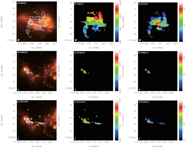
Figure 4.— The same as Figure 2 but for (a, b, and c) ¹²CO (3–2), (d, e, and f) HCN (4–3), and (g, h, and i) HCO⁺ (4–3). (a) The contours are 2, 4, 8, 16, 32, 64, 128, and 170 Jy km s^-1 (d) The contours are 0.04, 0.08, 0.16, 0.32, 0.64, 1.28, and 1.80 Jy km s^-1. (g) The contours are 0.04, 0.08, 0.16, 0.32, 0.64, 1.28, and 2.40 Jy km s^-1.

The ¹²CO (1–0) velocity field map of VV 114 (Figure 2b) shows a significantly broad velocity range across the galaxy disks ($\simeq$ 600 km s^-1). The SE arm has a blue-shifted velocity from 5650 km s^-1 to 5920 km s^-1, while the NW arm has a red-shifted velocity from 5950 km s^-1 to 6160 km s^-1. One possibility for the larger velocity width in the SE arm may be a highly inclined tidal arm. Two other arm-like features are also detected in the ¹²CO (1–0) observations. One arm is located $\simeq$ 4$\farcs$0 northeast of the eastern nucleus and shows an arc around the eastern nucleus in the velocity range of 5810 km s^-1 to 6180 km s^-1. The other arm is located $\simeq$ 10$\farcs$0 west of the SE arm and has a strong peak ($\simeq$ 262.5 $\pm$ 1.0 Jy km s^-1) in the velocity range of 5610 km s^-1 to 5900 km s^-1.

The overlap region has the highest velocity dispersion ($\simeq$ 110 km s^-1) (Figure 2c). The NW arm has an average velocity dispersion of $\simeq$ 30 km s^-1, while the SE arm has $\simeq$ 40 km s^-1. These values are significantly higher than the dispersions seen in Giant Molecular Clouds (GMCs) in the LMC (2 – 14 km s^-1; Minamidani et al., 2008; Fujii et al., 2014) and slightly higher than that in Giant Molecular Associations (GMAs) in the Antennae galaxy (6 – 36 km s^-1; Ueda et al., 2012). We suggest that the main contribution to the ¹²CO (1–0) velocity dispersion is inter cloud turbulent medium along the tidal arm, and/or shocked region induced by the tidal interaction, rather than the velocity dispersion of the GMCs/GMAs.

3.1.2 ¹³CO (1–0)

The integrated intensity, velocity field, and velocity dispersion maps of ¹³CO (1–0) are shown in Figures 2d, 2e, and 2f, respectively. The integrated ¹³CO (1–0) intensity map of VV 114 (Figure 2d) shows a filamentary structure across the galaxy disks, which is consistent with the region where the ¹²CO (1–0) filament is detected. The total ¹³CO (1–0) integrated intensity is 5.9 $\pm 0.4$ Jy km s^-1. The strongest peak is located $\simeq$ 4$\farcs$2 southwest of the eastern nucleus. The ¹³CO (1–0) velocity field map of VV 114 (Figure 2e) shows a narrower velocity range (5670 – 6000 km s^-1) than that of the ¹²CO (1–0) emission (5600 – 6200 km s^-1). This suggests that the ¹³CO (1–0) emission mainly comes from two components, the eastern galaxy and the blue-shifted component of the overlap region. The ¹³CO (1–0) velocity dispersion map of VV 114 (Figure 2f) shows a high velocity dispersion component ($\sim$ 100 km s^-1) between the eastern nucleus and the overlap region. This significant velocity dispersion may be caused by a superposition of clouds (see the double-peak spectrum at R39 shown in Appendix A.3).

3.1.3 CS (2–1) and CH₃OH (2_k–1_k)

The CS (2–1) and CH₃OH (2_k–1_k) lines are only detected at the overlap region (Figures 2g, 2h, 2i, 3a, 3b, and 3c). This is the first detection of the CH₃OH (2_k–1_k) emission in a merger-induced overlap region. We observed the blended set of 2₁ – 1₁ ($\nu_{\rm{rest}}$ = 96.756 GHz, $E_{\rm{up}}/k$ = 28.0 K), 2₀ – 1₀ E ($\nu_{\rm{rest}}$ = 96.745 GHz, $E_{\rm{up}}/k$ = 20.1 K), 2₀ – 1₀ A⁺ ($\nu_{\rm{rest}}$ = 96.741 GHz, $E_{\rm{up}}/k$ = 7.0 K), and 2_-1 – 1_-1 E ($\nu_{\rm{rest}}$ = 96.739 GHz, $E_{\rm{up}}/k$ = 12.5 K), thermal transitions of CH₃OH (hereafter designated the 2_k – 1_k transition). The distribution of these molecular lines is clearly different from the other dense gas tracers detected in the current program. The peaks of CS (2–1) and CH₃OH (2_k–1_k) are coincident with one of the peaks of ¹³CO (1–0) to within 0$\farcs$5. The total CS (2–1) and CH₃OH (2_k–1_k) integrated intensities are 0.4 $\pm$ 0.1 Jy km s^-1 and 0.5 $\pm$ 0.1 Jy km s^-1, respectively. The signal to noise is too low to resolve the velocity structure.

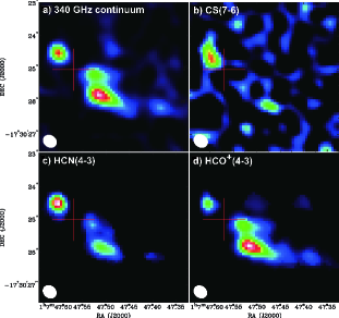
Figure 5.— (a) 340 GHz continuum flux image of VV 114E. The flux in color scale ranges from 0 mJy beam^-1 to 3.4 mJy beam^-1. (b) CS (7–6) integrated intensity image of VV 114E. The flux in color scale ranges from 0 Jy km s^-1 to 0.45 Jy km s^-1. (c) HCN (4–3) integrated intensity image of VV 114E. The flux in color scale ranges from 0 Jy km s^-1 to 2.0 Jy km s^-1. (d) HCO⁺ (4–3) integrated intensity image of VV 114E. The flux in color scale ranges from 0 Jy km s^-1 to 2.8 Jy km s^-1. The beam size of each line and continuum is shown in the bottom-left of the images (Table 2). The red cross shows the position of the eastern nucleus defined by the peak position of the Ks-band observation (Tateuchi et al., 2012).

3.1.4 CN (1_3/2–0_1/2) and CN (1_1/2–0_1/2)

Two radical CN rotational transitions N = 1 – 0 (J = 3/2 – 1/2 and 1/2 – 1/2) are detected at the eastern nucleus. The $J$ = 3/2 – 1/2 transition is extended toward the overlap region (Figures 3d, 3e, 3f, 3g, 3h, and 3i). We can not resolve their multiplet because of the coarse frequency resolution (11.5 MHz $\simeq$ 30 km s^-1). Because the critical density of CN is high ($\sim$ 10⁶ cm^-3), the CN emission mainly comes from denser gas regions than regions traced by ¹²CO (1–0). The J = 3/2 – 1/2 transition shows a similar distribution to the ¹³CO (1–0) emission, but it is less extended over the overlap region. The total CN (1_1/2–0_1/2) and CN (1_3/2–0_1/2) integrated intensities are 2.0 $\pm$ 0.1 Jy km s^-1 and 5.4 $\pm$ 0.3 Jy km s^-1, respectively. The highest velocity dispersion in the CN (1_3/2–0_1/2) image is also detected between the eastern nucleus and the overlap region, and this is likely caused by a superposition of clouds similar to the case of the ¹³CO (1–0) image (see Appendix  A.3).

3.2. Line Emission in Band 7

3.2.1 ¹²CO (3–2)

The ¹²CO (3–2) emission maps are presented in Figure 4. The estimated missing flux in our ALMA observation is 21 $\pm$ 1 % (James Clerk Maxwell Telescope (JCMT): 2956 $\pm$ 133 $\rm{Jy~{}km~{}s^{-1}}$ and ALMA: 2343.7 $\pm$ 4.7 $\rm{Jy~{}km~{}s^{-1}}$; Wilson et al., 2008; Saito et al., 2013). Although our ¹²CO (3–2) observation recovers more flux than the Submillimeter Array (SMA) observation (1530 $\pm$ 16 $\rm{Jy~{}km~{}s^{-1}}$; the missing flux = 48 $\pm$ 15 %; Wilson et al., 2008), there are significant negative sidelobes at the north and south of the image which is likely the cause of missing flux. We made the CLEANed image with a uniform uv weighting to minimized the sidelobe level (Thompson et al., 2001).

The ¹²CO (3–2) integrated intensity map of VV 114 (Figure 4a) shows two arm-like structures and a filamentary structure similar to the ¹²CO (1–0) image, and the strongest peak is at $\simeq$ 5$\farcs$5 west of the eastern nucleus. The global gas distribution is consistent with the previous ¹²CO (3–2) observations (Iono et al., 2004; Wilson et al., 2008). The ¹²CO (3–2) velocity field map of VV 114 (Figure 4b) also shows significant broad velocity range across the galaxy disks ($\simeq$ 600 km s^-1), similar to the ¹²CO (1–0) velocity field map. The SE arm has a blue-shifted velocity from 5650 km s^-1 to 5920 km s^-1, while the NW arm has a red-shifted velocity from 5950 km s^-1 to 6160 km s^-1. Other two arm-like features are also detected. One located $\simeq$ 4$\farcs$0 northeast of the eastern nucleus shows an arc around the eastern nucleus and has red-shifted velocities from 5810 km s^-1 to 6180 km s^-1. This arm coincides with the NE arm detected in the ¹²CO (1–0). The other one located at $\simeq$ 10$\farcs$0 west of the SE arm has a strong peak ($\simeq$ 262.5 $\pm$ 0.9  Jy km s^-1) and blue-shifted velocities from 5610 km s^-1 to 5900 km s^-1. This arm also coincide with the SW arm detected in the ¹²CO (1–0). From the ¹²CO (3–2) velocity dispersion map of VV 114 (Figure 4c), we find that the overlap region has the highest velocity dispersion ($\simeq$ 110 km s^-1). The velocity dispersion of the NW arm is $\simeq$ 30 km s^-1, while the SE arm is $\simeq$ 60 km s^-1.

Figure 6.— (a) The 110 GHz continuum flux image overlaid on the HST/ACS/F435W image of VV 114. The contours are 0.10, 0.20, 0.40, 0.80, and 1.60 mJy beam^-1. The red crosses show the positions of the nuclei defined by the peak positions of the Ks-band observation (Tateuchi et al., 2012). (b) The low resolution 340 GHz continuum flux image overlaid on the HST/ACS/F435W image of VV 114. The contours are 0.22, 0.44, 0.88, 1.76, 3.52, and 7.04 mJy beam^-1. A strong point source at the eastern edge of the image is a distant star-forming galaxy, ALMA J010748.3 – 173028 (see Tamura et al., 2014). (c) The high resolution 340 GHz continuum flux image overlaid on the HST/ACS/F435W image of VV 114. The contours are 0.14, 0.28, 0.56, 1.12, and 2.24 mJy beam^-1. The red cross shows the position of the eastern nucleus defined by the peak position of the Ks-band observation (Tateuchi et al., 2012). The beam size of each continuum is shown in the bottom-left of the images (Table 2).

3.2.2 HCN (4–3) and HCO⁺ (4–3)

The HCN (4–3) and HCO⁺ (4–3) images are shown in Figures 4d, 4e, 4f, 4g, 4h, and 4i. While the HCN (4–3) emission is only seen near the eastern nucleus of VV 114 and is resolved into four peaks, the HCO⁺ (4–3) emission is more extended and has at least 10 peaks in the integrated intensity map. The total integrated intensities of HCO⁺ (4–3) and HCN (4–3) are 15.3 $\pm$ 0.4 Jy km  s^-1 and 4.4 $\pm$ 0.2 Jy km s^-1, respectively. The higher HCO⁺ (4–3) flux observed with the SMA (17 $\pm$ 2 mJy, Wilson et al., 2008) using a 2$\farcs$8 $\times$ 2$\farcs$0 beam is likely attributed to missing flux by the ALMA observation. A compact component in the eastern nucleus is unresolved with the current resolution, and the upper limit to the size is 200 pc. The HCN (4–3) emission is not detected in the overlap region, where both the high ¹²CO (1–0) velocity dispersion and the significant CH₃OH (2_k–1_k) and HCO⁺ (4–3) detection suggest the presence of shocked gas (Krips et al., 2008). We concluded in paper I from their source size, line widths, and the relative strengths of HCN (4–3) and HCO⁺ (4–3) that the unresolved eastern nucleus harbors an obscured AGN, and the dense clumps in the western galaxy are related to extended starbursts.

3.2.3 CS (7–6)

The CS (7–6) emission has the highest critical density ($n_{\rm{cr}}$ $\simeq$ 10⁷ cm^-3) of all of the lines detected in our observations. The CS (7–6) emission is marginally (S/N $\sim$ 4) detected at the eastern nucleus (Figure 5), and the total flux is 0.5 $\pm$ 0.1 Jy km s^-1.

3.3. Continuum Emission

The continuum image at 110 GHz shows a filamentary structure similar to the molecular line image (Figure 6a). We construct low resolution (1$\farcs$33 $\times$ 1$\farcs$12) and high resolution (0$\farcs$45 $\times$ 0$\farcs$38) images of the 340 GHz continuum (Figures 6b, and 6c) using the combined data (compact + extended) and the extended configuration data, respectively. We find that the filamentary structure and the unresolved eastern nucleus are both present in dust continuum. The total flux of the 110 GHz and the low resolution 340 GHz continuum emission are 10.3 $\pm$ 0.2 mJy and 38.6 $\pm$ 0.3 mJy, respectively. The estimated missing flux relative to the JCMT 340 GHz observation (Wilson et al., 2008) is 75 $\pm$ 4 % (SMA: 79 $\pm$ 7 %). The difference in the recovered flux between ¹²CO (3–2) and 340 GHz continuum emission may be caused by the difference in the distribution. The 110 GHz and 340 GHz continuum emission is detected at the eastern nucleus (S/N $\sim$ 50 and 70) and the filamentary structure (S/N $\sim$ 8 and 24) identified in the ¹³CO (1–0) image, both with high significance.

4. Spatially resolved line ratios

We assign 39 “R” boxes (2$\farcs$0 $\times$ 2$\farcs$0; R1 – R39; see Figure 7) for the band 3 and ¹²CO (3–2) data and 15 smaller “S” boxes (1$\farcs$2 $\times$ 1$\farcs$2; S0 – S14; see Figure 8) for the rest of the data to estimate the physical parameters, such as the molecular gas mass ($M_{\rm{H_{2}}}$), dense gas mass ($M_{\rm{dense}}$), dust mass ($M_{\rm{dust}}$), star formation rate (SFR), kinetic temperature ($T_{\rm{kin}}$), gas density ($n_{\rm{H_{2}}}$), gas column density ($N(\rm{H_{2}})$), and molecular abundance relative to H₂ ([$X$]/[H₂]). The positions of the boxes are chosen to cover the CO (3–2) emission (R1 – R39) and the HCO⁺ (4–3) emission (S0 – S14). The sizes of the boxes are chosen such that they are comparable to the beam size. Before deriving the parameters and line ratios at each box, we first matched the $uv$ range between our data set and reconstructed the integrated intensity image of each line. The shortest baseline lengths are set to 13.5 k$\lambda$ and 40.0 k$\lambda$ for the molecular lines in the band 3 and the band 7, respectively, and the images are convolved into the same resolution (2$\farcs$0 $\times$ 1$\farcs$5 with a P.A. of 83 deg, 1$\farcs$2 $\times$ 1$\farcs$0 with a P.A. of 119 deg). For each ratio, the two integrated intensity images were expressed in the units of K km s^-1 before calculating the ratio at locations where both lines are detected above 3 $\sigma$. The derived box-summed spectra are listed in Appendix A.3. We carried out a multi Gaussian fit (one - three components) to reproduce the box-summed spectra, and labeled the components as “a”, “b”, and “c” from the bluest peak (e.g., the bluest peak at R21 is labeled as R21a).

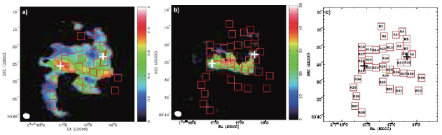
Figure 7.— (a) The $R_{3-2/1-0}$ image. The ratio in color scale ranges from 0 to 1. The white crosses show the positions of the nuclei defined by the peak positions of the Ks-band observation (Tateuchi et al., 2012). (b) The $R_{12/13}$ image. The ratio in color scale ranges from 0 to 40. (c) Locations of 39 boxes (R1 – R39) that are used to calculate the line ratios and physical parameters. For each ratio, the two integrated intensity images were convolved to the same resolution and expressed in units of K km s^-1 before calculating the ratio at locations where both lines are detected above 3 $\sigma$. The black crosses show the positions of the nuclei defined by the peak positions of the Ks-band observation (Tateuchi et al., 2012). The beam size of each line ratio is shown in the bottom-left of the images.

4.1. ¹²CO (3–2)/¹²CO (1–0), $R_{3-2/1-0}$

The ¹²CO (3–2)/¹²CO (1–0) ratio, $R_{3-2/1-0}$, can be used as an indicator of the dense/warm gas content relative to the total molecular gas. The $R_{3-2/1-0}$ of VV 114 varies from 0.2 to 0.8, as shown in Figure 7 (left) and Table 6. This range is larger than the same ratios derived for normal spirals, which is typically 0.15 – 0.5 when observed with a similar linear resolution (Warren et al., 2010). At the edge and the center of the filament, $R_{3-2/1-0}$ is higher (0.53 – 0.69) than the highest peaks of each arm ($\sim$ 0.4). This suggests that the CO emitting gas at the filament have higher excitation conditions than normal spirals, while the conditions of each arm of VV 114 are consistent with arms and nuclei of normal spirals. The $R_{3-2/1-0}$ at the eastern nucleus is 0.76 $\pm$ 0.01. It is suggested that the $R_{3-2/1-0}$ is much higher (3.12 $\pm$ 0.03 in NGC 1068; Tsai et al., 2012) for gas surrounding an AGN, and the low $R_{3-2/1-0}$ in VV 114 may be due to the difference in filling factor (160 $\times$ 140 pc beam averaging for NGC 1068, while 800 pc box averaging for VV 114). It is possible, however, that the nuclear excitation conditions are different from source to source.

4.2. ¹²CO (1–0)/¹³CO (1–0), $R_{12/13}$

In general, the ¹²CO lines has higher optical depths than the ¹³CO (1–0) line. Therefore, the measured ¹²CO (1–0)/¹³CO (1–0) line intensity ratio, $R_{12/13}$, gives a lower limit to the CO/¹³CO abundance ratio (hereafter [CO]/[¹³CO]). We present the $R_{12/13}$ image of VV 114 in Figure 7 (center). The $R_{12/13}$ increases from the arms ($<$ 17) to the filament (15 – 32). Observationally, $R_{12/13}$ increases towards the central region of galaxies (Aalto et al., 1995), where the gas is generally warmer and denser. Aalto et al. (1995) suggest that the moderate optical depth of ¹²CO (1–0) emission and/or the high [CO]/[¹³CO] environment can increase the $R_{12/13}$ in nuclei of U/LIRGs. In order to understand which of the two (optical depths or abundances) is dominant, we calculated and mapped the optical depth of the ¹²CO (1–0) and the ¹³CO (1–0) as shown in Table 14 and Figure 10. We provide an interpretation of these results in §5.2.

4.3. HCN (4–3)/HCO⁺ (4–3), $R_{\rm{HCN/HCO^{+}}}$

In paper I, the HCN (4–3) and HCO⁺ (4–3) maps of VV 114 allowed us to investigate the central region at 200 pc resolution for the first time, and we find that both the HCN (4–3) and HCO⁺ (4–3) in the eastern nucleus are compact ($<$ 200 pc), and broad [290 km s^-1 for HCN (4–3)]. We present the HCN (4–3)/HCO⁺ (4–3), $R_{\rm{HCN/HCO^{+}}}$, image of VV 114 in Figure 8. From the higher $R_{\rm{HCN/HCO^{+}}}$ along with the past X-ray and NIR observations, we suggest the presence of an obscured AGN in the eastern nucleus. We also detect a 3 – 4 kpc long filament of dense gas, which is likely to be tracing the active star formation triggered by the ongoing merger, and this is consistent with the results from the numerical model by Teyssier et al. (2010) who predict that the fragmentation and turbulent motion of dense gas across the merging disk is responsible for forming dense gas clumps with masses of 10⁶ – 10⁸ M_⊙.

We present the $R_{\rm{HCN/HCO^{+}}}$ image in Figure 8. The overlap region does not show significant HCN (4–3) emission, and we provide the 3 $\sigma$ upper limit in Table 7. Three out of the four boxes (i.e., S1 – S3) in the eastern nucleus have low $R_{\rm{HCN/HCO^{+}}}$ ($<$ 0.5) whereas S0 has a high $R_{\rm{HCN/HCO^{+}}}$ (1.34 $\pm$ 0.09). It is suggested that such a high value is only produced around AGN environments (e.g., Kohno et al., 2001; Harada et al., 2013; Iono et al., 2013; Izumi et al., 2013; Imanishi & Nakanishi, 2014).

5. Derivation of physical parameters

In this section, we derive the molecular gas mass (§5.1), and the physical parameters using the radiative transfer code RADEX (§5.2) for each box defined in §4. The column density is derived using the optically thin ¹³CO line under the LTE assumption. We estimate the beam filling factor $\Phi_{\rm{A}}$ and the relative molecular abundance of molecule $X$ (hereafter expressed as [$X$]/[H₂]) (§5.3). Finally, we calculate the dust mass using the 340 GHz continuum emission (§5.4).

5.1. Molecular Gas Mass Derivation

The molecular gas mass M_X is derived by;

$$M_{\rm{X}}=\alpha_{\rm{X}}\>L^{\prime}_{\rm{X}}\>[\rm{M}_{\odot}],$$ (1)

where $\alpha_{\rm{X}}$ is the molecular line luminosity-to-H₂ mass conversion factor and $L\arcmin_{\rm{X}}$ is the velocity integrated flux (Solomon & Vanden Bout, 2005). We use the conversion factor known to be appropriate for U/LIRGs ($\alpha_{\rm{CO}}$ = 0.8 M${}_{\odot}~{}\rm{(K~{}km~{}s^{-1}~{}pc^{2})^{-1}}$; Downes & Solomon, 1998). This is consistent with the value derived by Sliwa et al. (2013) in VV 114 ($\alpha_{\rm{CO}}$ = $0.5^{+0.6}_{-0.3}$ M${}_{\odot}~{}\rm{(K~{}km~{}s^{-1}~{}pc^{2})^{-1}}$). The molecular gas mass derived at the boxes defined in §4 ranges between 0.2 $\times$ 10⁸ $\left(\frac{\alpha_{\rm{CO}}}{0.8}\right)$ and 4.8 $\times$ 10⁸ $\left(\frac{\alpha_{\rm{CO}}}{0.8}\right)$ M_⊙ (Table 10). We also calculate the dense gas mass $M_{\rm{dense}}$ using $\alpha_{\rm{HCN}}$ = 10 M${}_{\odot}~{}\rm{(K~{}km~{}s^{-1}~{}pc^{2})^{-1}}$ (Gao & Solomon, 2004) and the HCN (4–3) luminosity which is converted to the HCN (1–0) luminosity using HCN (4–3)/HCN (1–0) = 0.63 (paper I; Imanishi et al., 2007). The dense gas mass ranges between 1.8 $\times$ 10⁶ $\left(\frac{\alpha_{\rm{HCN}}}{10}\right)$ and 3.8 $\times$ 10⁷ $\left(\frac{\alpha_{\rm{HCN}}}{10}\right)$ M_⊙ (Table 11).

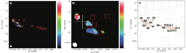
Figure 8.— (a) The $R_{\rm{HCN/HCO^{+}}}$ image. The ratio in color scale ranges from 0 to 1. The white cross shows the position of the eastern nucleus defined by the peak position of the Ks-band observation (Tateuchi et al., 2012). (b) The $R_{\rm{HCN/HCO^{+}}}$ image near the nucleus of VV 114E. The ratio in color scale also ranges from 0 to 1. (c) Locations of 15 boxes (S0 – S14) that are used to calculate the line ratios and physical parameters. For each ratio, the two integrated intensity images were convolved to the same resolution and expressed in units of K km s^-1 before calculating the ratio at locations where both lines are detected above 3 $\sigma$. The black cross shows the position of the eastern nucleus defined by the peak position of the Ks-band observation (Tateuchi et al., 2012). The green open squares are the “R” boxes shown in Figure 7c.

We note that the CO luminosity-to-H₂ mass conversion factor, $\alpha_{\rm{CO}}$, is very uncertain, and varies significantly from source to source (0.4 – 0.8 for LIRGs; Downes & Solomon, 1998; Yao et al., 2003; Papadopoulos et al., 2012; Bolatto et al., 2013). It may be possible that $\alpha_{\rm{CO}}$ varies from region to region within a galaxy. While one would ideally adopt a spatially varying $\alpha_{\rm{CO}}$ for a better quantification of the H₂ mass, such a study is beyond the scope of this present paper. For simplicity, here we adopt a constant $\alpha_{\rm{CO}}$ across all regions in VV 114, bearing in mind that the uncertainties could be as large as a factor of two. The same applies to $\alpha_{\rm{HCN}}$ (Gao & Solomon, 2004).

5.2. Radiative Transfer Analysis using $\rm{RADEX}$

We used the non-LTE radiative transfer code RADEX (van der Tak et al., 2007) and varied the parameters until the residuals between the observed line fluxes and the modeled line fluxes are minimized in a $\chi^{2}$ sense. We assumed a uniform spherical geometry ($dv$ = 1.0 $\rm{km~{}s^{-1}}$), and derived the physical conditions of molecular gas ($T_{\rm{kin}}$, $n_{\rm{H_{2}}}$, and $N(\rm{H}_{2})$). RADEX uses an escape probability approximation to solve the non-LTE excitation assuming that all lines are from the same region. Since the molecular lines in the band 7 have significantly higher critical densities than that in the band 3, we used two sets of molecular lines; (case 1) 2$\farcs$0 box-summed ¹²CO (1–0), ¹³CO (1–0), and ¹²CO (3–2), and (case 2) 1$\farcs$2 box-summed HCN (4–3), HCO⁺ (4–3), ¹²CO (3–2), and ¹²CO (1–0), to solve for the degeneracy of the physical parameters. In case 2, we made the uv and beam-matched HCN (4–3), HCO⁺ (4–3), and ¹²CO (3–2) images (1$\farcs$2 $\times$ 1$\farcs$0 resolution with the P.A. = 119 deg.), and we defined three HCO⁺ (4–3) peaks as E0, E1, and E2 (Figure 9). We also use the $uv$ and beam-matched ¹²CO (1–0) data to constrain the $N(\rm{H}_{2})$, allowing us to vary the [HCN]/[HCO⁺] in case 2. All line parameters, such as the upper state energies and the Einstein coefficients, were taken from the Leiden Atomic and Molecular Database (LAMDA; Schöier et al., 2005). In order to find the set of physical parameters that can reproduce the observed line intensities, we run RADEX by varying $T_{\rm{kin}}$, $n_{\rm{H_{2}}}$, and $N(\rm{H_{2}})$ for case 1, and $T_{\rm{kin}}$, $n_{\rm{H_{2}}}$, and [HCN]/[HCO⁺] for case 2. The adopted $N(\rm{H_{2}})$ are 10^21.2, 10^21.6, and 10^21.5 cm^-2, at E0, E1, and E2, respectively.

We varied the gas kinetic temperature within a range of $T_{\rm{kin}}$ = 5 – 300 K using steps of d$T_{\rm{kin}}$ = 5 K, and a gas density of $n_{\rm{H_{2}}}$ = $10^{2}$ – $10^{5}~{}\rm{cm^{-3}}$ using steps of d$n_{\rm{H_{2}}}$ = $10^{0.1}~{}\rm{cm^{-3}}$. For case 1, we fixed [¹³CO]/[H₂] = 1.4 $\times$ 10^-6 (Davis et al., 2013) and [CO]/[${}^{13}\rm{CO}$] = 70, which are the Galactic values (Wilson & Rood, 1994). In case 2, we changed the parameters, $T_{\rm{kin}}$ = 5 – 400 K using steps of d$T_{\rm{kin}}$ = 5 K, $n_{\rm{H_{2}}}$ = $10^{3}$ – $10^{7}~{}\rm{cm^{-3}}$ using steps of d$n_{\rm{H_{2}}}$ = $10^{0.1}~{}\rm{cm^{-3}}$, and fixed [CO]/[H₂] = 1.0 $\times$ 10^-4 and [HCO⁺]/[H₂] = 1.0 $\times$ 10^-9, which are the standard values observed in Galactic molecular clouds (Blake et al., 1987). We varied [HCN]/[HCO⁺] from 1 – 10, in steps of one. The parameters we used are summarized in Table 9. We list the results that are within the 95 % confidence level with 3-degree of freedom ($\chi^{2}<7.81$) (Tables 12 and 13). Finally, we created velocity-averaged channel maps of $n_{\rm{H_{2}}}$ and the optical depth of the transitions (Figure 10).

We note that the uncertainty of the $N(\rm{H_{2}})$ for case 2 did not strongly affect the results, while that of the [CO]/[${}^{13}\rm{CO}$] for case 1 changed. The effect of varying the [CO]/[${}^{13}\rm{CO}$] will be discussed in §5.2.1. Future multi-transition HCN/HCO⁺/CO/¹³CO imaging will help us to derive these parameters directly.

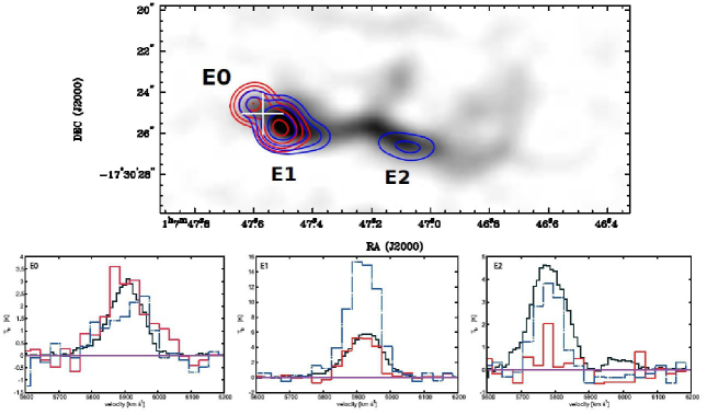
Figure 9.— (top) The $uv$- and beam-matched (grey color) ¹²CO (3–2), (red contour) HCN (4–3), and (blue contour) HCO⁺ (4–3) images. The integrated intensity of the ¹²CO (3–2) in color scale ranges from 0 Jy km s^-1 to 100 Jy km s^-1. The contours are 5, 10, 20, 40, and 50 Jy km s^-1 for HCN (4–3), and 12, 24, 48, and 96 Jy km s^-1 for HCO⁺ (4–3). The white cross shows the position of the eastern nucleus defined by the peak position of the Ks-band observation (Tateuchi et al., 2012). (bottom) 1$\farcs$2 box-summed spectra of (black line) ¹²CO (3–2), (red dashed line) HCN (4–3) $\times$ 10, and (blue dashed line) HCO⁺ (4–3) $\times$ 10 at the each box, labeled E0 – E2. The spectra are taken from the ALMA data cubes after correcting the cubes for the primary beam attenuation and convolving them to 1$\farcs$2 $\times$ 1$\farcs$0 resolution (P.A. = 119 deg.).

5.2.1 Case 1

The (box-averaged) kinetic temperature near the eastern nucleus (R21a) is constrained to within 25 – 90 K (the best fit is 50 K), as shown in Table 12. The $T_{\rm{ex}}$ (58.8 $\pm$ 2.9 K) obtained from the LTE assumption at R21a (see §5.3) is higher than the best-fitted $T_{\rm{kin}}$. In fact, we also find five regions (R10b, R11b, R14, R16, and R25a) that show similarly high excitation temperatures. Four out of five regions are in the central filament. In general, spontaneous emission dominates over collisional excitation in sub-thermally excited conditions, and hence $T_{\rm{ex}}$ should be lower than $T_{\rm{kin}}$. One reason for this discrepancy could be attributed to the incorrect assumption of [CO]/[¹³CO]. By varying this abundance ratio, we find that the temperature reversal (i.e. $T_{\rm{kin}}>T_{\rm{ex}}$) occurs only when [CO]/[¹³CO] $>$ 150. This is consistent with the results obtained by Sliwa et al. (2013) who used RADEX along with their multi CO and ¹³CO line data to find evidence of a cold/dense molecular gas component with extremely high [CO]/[¹³CO] of 229, which is 3 times higher than that of the Galactic value (Wilson & Rood, 1994).

The derived $T_{\rm{kin}}$ at the other regions are generally higher than 100 K. The derived $T_{\rm{ex}}$ in each region are typically 10 – 40 K, which may suggest sub-thermal conditions. The kinetic temperatures derived at the SE and NW arms are estimated to be $<$ 90 K, with higher temperature at the NW arm. The NW arm is also associated with relatively strong Pa$\alpha$ emission and $K$s-band emission, which is consistent with the higher relative temperature due to star-forming activities (Minamidani et al., 2008). However, this is inconsistent with the general understanding that strong tidal shear in tidal arms prevents active star formation to occur (Aalto et al., 2010).

The derived $n_{\rm{H_{2}}}$ in most of the boxes are less than 10^3.0 cm^-3, which is consistent with the critical densities of the low-$J$ CO lines observed here. The highest density of 10^3.4 – 10^5.0 cm^-3 is estimated at R21a, and this is consistent with the location of the eastern nucleus. Since we also observed the strongest HCN (4–3) and HCO⁺ (4–3) emission at R21a at the same line-of-sight velocity (Iono et al., 2013, see also Appendix A.3), it is possible that the main contribution to the CO emission at R21a arises from dense gas (10^3.4 – 10^5.0 cm^-3) near the eastern nucleus, with a minor contribution from the diffuse gas clouds along the same line of sight observed within the same beam. In contrast to the eastern nucleus, the boxes that cover the western galaxy (R1 – R11 and R26 – R29) show moderately dense condition of 10^2.0 – 10^4.0 cm^-3. This extended and moderately dense gas is associated with the disk-like structure seen in optical images (Evans, 2008), and the star formation traced in Pa$\alpha$ emission and UV/X-ray emission (Grimes et al., 2006; Tateuchi et al., 2012). We note that the strongest off-nuclear Pa$\alpha$ peak (R27 in Table 10; SFR = 3.15 $\pm$ 0.05 M_⊙ yr^-1) coincides with relatively low gas density ($\sim$ 10^3.0 cm^-3). The density of the surrounding region labeled R25a is similar (10^3.5 – 10^5.0 cm^-3) and this is comparable to the nucleus of the eastern galaxy. The secondary Pa$\alpha$ peak (R29; SFR = 0.92 $\pm$ 0.05 M_⊙ yr^-1) is not associated with any molecular line emission.

It is usually believed that the ¹²CO (1–0) emission is optically thick ($\tau_{\rm{CO}}\gg 1$), while the ¹³CO (1–0) emission is optically thin ($\tau_{\rm{{}^{13}CO}}\ll 1$) even in luminous mergers (Davis et al., 2013). In most regions, we find that the optical depth of the ¹²CO (1–0) line is $\gg$ 1 (Figure 10). In contrast, the ¹²CO (1–0) opacity at the eastern nucleus and the filament is moderately optically thick ($\tau_{\rm{CO}}$ $\sim$ 1). However, the elevated $R_{12/13}$ at the eastern nucleus (see §4) cannot be explained by the relatively low ¹²CO (1–0) opacity alone (the opacity has to be $\tau_{\rm{CO}}$ $\ll$ 0.1; see also Wilson et al. (2009)). Finally, we find that indeed the ¹³CO (1–0) emission is optically thin ($\tau_{\rm{{}^{13}CO}}\ll 1$) averaged over the whole galaxy, except for the southern dust lane ($\tau_{\rm{{}^{13}CO}}$ = 0.3 – 1.5).

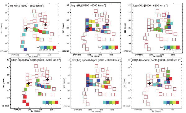
Figure 10.— The channel maps of the box-averaged RADEX modeling based on the ¹²CO (1–0), ¹³CO (1–0), and ¹²CO (3–2). (top) The best fitted values of logarithmic gas density of the ¹²CO (1–0) emission. The value in color scale ranges from 2.0 to 4.0 cm^-3. (bottom) The best fitted values of optical depth of the ¹²CO (1–0) emission. The value in color scale ranges from 0 to 9. The black crosses show the positions of the nuclei defined by the peak positions of the Ks-band observation (Tateuchi et al., 2012). The open squares are regions which we cannot solve the RADEX calculations because of non-detection of the ¹²CO (1–0), ¹³CO (1–0), or ¹²CO (3–2) emission.

From these results, we suggest that the peak of the molecular gas in the central 800 pc of the eastern galaxy is cold ($T_{\rm{kin}}$ = 25 – 90 K), dense ($n_{\rm{H_{2}}}$ = 10^3.4 – 10^5.0 cm^-3), and moderately optically thick ($\tau_{\rm{CO(1-0)}}$ $\sim$ 3), while peaks in the overlap region are warm ($T_{\rm{kin}}$ $>$ 50 K, best-fitted $T_{\rm{kin}}$ is 95 and 175 K at R39a and R39b, respectively), moderately dense ($n_{\rm{H_{2}}}$ = 10^2.3 – 10^4.1 cm^-3), and moderately optically thick ($\tau_{\rm{CO(1-0)}}$ $\sim$ 1). The derived density of the eastern galaxy is slightly higher than the range of values found in U/LIRGs using low-$J$ CO emission with$\sim$ kpc resolution ($n_{\rm{H_{2}}}$ = 10^2.3 – 10^4.3 cm^-3; Downes & Solomon, 1998). In addition, the low opacities predicted from these analyses are consistent with earlier results that investigate the opacities in M82 ($\tau$ = 0.5 – 4.5; Mao et al., 2000) and U/LIRGs ($\tau$ = 3 – 10; Downes & Solomon, 1998), and the central region of NGC 6240 ($\tau$ = 0.2 – 2; Iono et al., 2007). However, the derived temperature of the eastern galaxy is inconsistent with the high values found in nearby starburst galaxies M82, NGC 253, and NGC 6240 (Wild et al., 1992; Jackson et al., 1995; Seaquist & Frayer, 2000; Iono et al., 2007). The disagreement is possibly due to the uncertainties in the [CO]/[¹³CO], or the difference in the observed molecular gas tracers.

5.2.2 Case 2

The values for $T_{\rm{kin}}$, $n_{\rm{H_{2}}}$, and the optical depth of HCN (4–3) and HCO⁺ (4–3) are shown in Table 8. The derived parameters for the unresolved component E0, are $T_{\rm{kin}}$ $>$ 100 K, $n_{\rm{H_{2}}}$ = 10^5.0 – 10^5.4 cm^-3, and [HCN]/[HCO⁺] $>$ 5. The lower limit to the kinetic temperature is higher than those of E1 and E2, mainly due to the unusually high $R_{\rm{HCN/HCO^{+}}}$ and $R_{\rm{HCN/CO}}$. In contrast to E0, the derived parameters near E1 show high H₂ densities ($n_{\rm{H_{2}}}$ = 10^5.6 – 10^5.9 cm^-3). The overlap region (E2), where the star-formation rate (1.70 $\pm$ 0.05 M_⊙ yr^-1) is lower than the eastern nucleus, has densities in the range of $n_{\rm{H_{2}}}$ = 10^5.0 – 10^5.6 cm^-3. Finally, the optical depths for the HCO⁺ (4–3) and HCN (4–3) lines are calculated for each gas clump, yielding $\tau_{\rm{HCN}}$ $\simeq$ 0.7 and $\tau_{\rm{HCO^{+}}}$ $\simeq$ 0.2 for E0, $\tau_{\rm{HCN}}$ $\simeq$ 0.2 and $\tau_{\rm{HCO^{+}}}$ $\simeq$ 0.6 for E1, and $\tau_{\rm{HCN}}$ $\simeq$ 0.4 and $\tau_{\rm{HCO^{+}}}$ $\simeq$ 0.4 for E2.

The higher linear resolution observations of HCN (4–3) and HCO⁺ (4–3) toward NGC 1097 (Izumi et al., 2013) revealed that the gas in the central region of NGC 1097 has $T_{\rm{kin}}$ = 70 – 550 K and $n_{\rm{H_{2}}}$ = 10^4.5 – 10^6.0 cm^-3. Moreover, by comparing to LVG models, Krips et al. (2008) found that HCN and HCO⁺ emission in AGN-dominated sources appears to emerge from regions with lower H₂ densities, higher temperatures, and higher HCN abundance relative to starburst-dominated (SB-dominated) galaxies. Our results obtained toward VV 114 are consistent with these previous results.

5.3. Filling factor and Column Density under LTE

In order to determine the bulk properties of the CO emitting gas, we used an excitation temperature analysis (Davis et al., 2013). The excitation temperature at each box can be calculated from

$$T_{\rm{ex}}=T_{0}\>\left(\ln\left[\left(\frac{T_{\rm{b,CO(1-0)}}}{\Phi_{\rm{A}}T_{0}(1-e^{-\tau_{\rm{CO}}})}+\frac{1}{e^{T_{0}/T_{\rm{bg}}}-1}\right)^{-1}+1\right]\right)^{-1}$$ (2)

where $T_{0}=h\nu/k$ [= 5.53 K for ¹²CO (1–0) emission], $\nu$ is the frequency of the transition, $h$ is the Planck’s constant, $k$ is the Boltzmann’s constant, $T_{\rm{b,CO(1-0)}}$ is the brightness temperature of ¹²CO (1–0) emission in Kelvin, $\tau_{\rm{CO}}$ is the optical depth of the ¹²CO (1–0) emission, and $T_{\rm{bg}}$ is the cosmic microwave background temperature (2.73 K). Using $T_{\rm{kin}}$ estimated from the RADEX calculation (§5.2), we estimate the beam filling factor $\Phi_{\rm{A}}$,

$$\Phi_{\rm{A}}=\frac{T_{\rm{b,CO(1-0)}}}{T_{\rm{kin}}}$$ (3)

The optical depth of the ¹²CO (1–0) emission is also estimated from the RADEX calculation in §5.2. Assuming that the ¹³CO and CO arise from the same molecular cloud, and that the ¹²CO (1–0) is optically thick, we estimate the optical depth of a given molecule using,

$$\tau_{\rm{X}}\simeq\ln\left[\left(1-\frac{T_{\rm{b},X}}{T_{\rm{b,CO(1-0)}}}\right)^{-1}\right]$$ (4)

where $\tau_{\rm{X}}$ is the optical depth of a given transition, and $T_{\rm{b,X}}$ is the observed brightness temperature for transition X. Using $T_{\rm{ex}}$ and $\tau_{\rm{X}}$, we estimate the column density for a given molecule from,

$$N_{\rm{X}}=\frac{3k}{8\pi^{3}\mu^{2}B(J+1)}\frac{\exp\left(\frac{2hJ(J+1)}{kT_{\rm{ex}}}\right)}{\left(1-\exp\left(-\frac{h\nu}{kT_{\rm{ex}}}\right)\right)}$$

$$\times\>\frac{\tau_{\rm{X}}}{1-e^{-\tau_{\rm{X}}}}\frac{1}{J(T_{\rm{ex}})-J(T_{\rm{bg}})}\int T_{\rm{R}}^{*}dV$$ (5)

$$J(T)=\frac{h\nu}{k}\frac{1}{\exp(h\nu/kT)-1}$$ (6)

where $\mu$ is the dipole moment, $B$ is the rotational constant, $J$ is the lower energy level, and $\int T_{\rm{R}}^{*}dV$ is the integrated intensity (Wilson et al., 2009). The derived column densities are listed in Tables 14 and 15.

5.4. Dust Mass and ISM Mass Derivation from 340 GHz continuum

We calculated the dust mass from the 340 GHz (880 $\mu$m) continuum emission (Table 3) using (Wilson et al., 2008),

$$M_{\rm{dust}}=74220\>S_{340}\>D_{\mathrm{L}}^{2}\frac{e^{\frac{17}{T_{d}}}-1}{\kappa_{340}}\>{\rm{M}_{\odot}}$$ (7)

where $S_{340}$ is the 340 GHz flux in Jy and $D_{\rm{L}}$ is the luminosity distance in Mpc. We assumed a dust emissivity, $\kappa_{340}=0.9~{}\rm{cm^{2}~{}g^{-1}}$, and the dust temperature $T_{\rm{d}}$ of 39.4 K (Wilson et al., 2008). The box-summed dust masses ranges between 2.0 $\times$ 10⁴ $\left(\frac{0.9}{\kappa_{340}}\right)$ and 2.8 $\times$ 10⁶ $\left(\frac{0.9}{\kappa_{340}}\right)$ M_⊙ (Table 10). We note that we used the Draine & Lee (1984) dust model for $\kappa_{340}$, because the $\kappa_{340}$ derived from observations has a large error (Henning et al., 1995).

Scoville et al. (2014) suggested that the submillimeter continuum emission traces the total ISM mass ($M_{\rm{ISM}}$), since the long wavelength Rayleigh-Jeans (RJ) tail of thermal dust emission is often optically thin. In order to compare the $M_{\rm{ISM}}$ with the $M_{\rm{H_{2}}}$ (see $5.1) using spatially-resolved data, we calculated the total ISM mass from the 340 GHz continuum emission (Scoville et al., 2014). For $\nu_{\rm{rest}}$ $\lesssim$ 1199 GHz,

$$S_{\rm{\nu_{obs}}}=0.83\frac{M_{\rm{ISM}}}{10^{10}\>\rm{M}_{\odot}}(1+z)^{4.8}\left(\frac{\nu_{\rm{obs}}}{353~{}\rm{GHz}}\right)^{3.8}$$

$$\times\frac{\Gamma_{\rm{RJ}}}{\Gamma_{0}}\left(\frac{\rm{Gpc}}{D_{\rm{L}}}\right)\rm{mJy}$$ (8)

where $S_{\rm{\nu_{obs}}}$ is the observed flux, $M_{\rm{ISM}}$ is the ISM mass, $\nu_{\rm{obs}}$ is the observed frequency, and $\Gamma_{\rm{RJ}}$ and $\Gamma_{0}$ are given by

$$\Gamma_{\rm{RJ}}(T_{d},\nu_{\rm{obs}},z)=\frac{h\nu_{\rm{obs}}(1+z)/kT_{d}}{e^{h\nu_{\rm{obs}}(1+z)/kT_{d}}-1}$$ (9)

$$\Gamma_{0}=\Gamma_{\rm{RJ}}(T_{d},353~{}\rm{GHz},0).$$ (10)

The derived box-summed ISM masses of VV 114 range between 5.2 $\times$ 10⁷ and 7.2 $\times$ 10⁸ M_⊙ (Table 10). This is comparable to the box-summed H₂ masses ($M_{\rm{H_{2}}}$ = (0.2 – 4.7) $\times$ 10⁸ $\left(\frac{\alpha_{\rm{CO}}}{0.8}\right)$ M_⊙). We find that the $M_{\rm{ISM}}$/$M_{\rm{H_{2}}}$ ratio is close to unity (0.5 – 2.0, the average $M_{\rm{ISM}}$/$M_{\rm{H_{2}}}$ = 0.9 $\pm$ 0.1), while the total $M_{\rm{ISM}}$/$M_{\rm{H_{2}}}$ ratio is 0.6 $\pm$ 0.1. This means that the spatially-resolved $M_{\rm{ISM}}$ is a good tracer of the “resolved” H₂ mass. However, the total $M_{\rm{ISM}}$ underestimates the H₂ mass (even using the $\alpha_{\rm{CO}}$ for ULIRGs to derive the $M_{\rm{H_{2}}}$) because the global distribution of the 340 GHz continuum emission is significantly different from that of the CO (1–0) emission (Figures 2 and 6). This difference between the 340 GHz continuum and the CO (1–0) is also seen in recent observations of nearby LIRGs (e.g., Sakamoto et al., 2014).

6. Discussion

6.1. Conditions of “Dense” Gas near the Eastern Nucleus

Our RADEX modeling yields lower molecular gas density near the AGN ($n_{\rm{H_{2}}}$ = 10^5.0 – 10^5.4 cm^-3) compared to the surrounding clumps (10^5.6 – 10^5.9 cm^-3). Similarly high values are obtained near AGNs in other galaxies (Alonso-Herrero et al., 2002; Wilson et al., 2003; Krips et al., 2008). Krips et al. (2008) suggest that the gas densities in AGN host galaxies ($<$ 10^4.5 cm^-3) are lower than starburst host galaxies (10^5.0 – 10^6.5 cm^-3), and a common interpretation relies on a clumpy ISM near star-forming regions (which reduces the filling factor) and a continuous ISM near the AGN. Since our current observations ($\sim$ 200 pc resolution) cover a significantly large area and the beam filling factor may be small ($\Phi_{\rm{A}}$ at E0, E1, and E2 are $\lesssim$ 0.03, 0.04 – 0.06 and 0.01 – 0.04, respectively), higher resolution observations ($<$ 0$\farcs$5) are required to confirm this scenario.

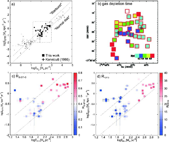
Figure 11.— (a) The Kennicutt-Scimidt law of VV 114 overlaid on other galaxies. Filled squares show regions of VV 114, while crosses show galaxies in the sample of Kennicutt (1998). The dashed line and the dotted line indicate the “starburst” sequence and “normal disk” sequence, respectively (Daddi et al., 2010). (b) Distribution of the box-averaged gas depletion time ($\tau_{\rm{gas}}$ = $\Sigma_{\rm{H_{2}}}/\Sigma_{\rm{SFR}}$). The gas depletion time in color scale ranges from 0 - 1 Gyr. The black crosses show the positions of the nuclei defined by the peak positions of the Ks-band observation (Tateuchi et al., 2012). The open square is a region which we cannot estimate the gas depletion time because of non-detection of the Pa$\alpha$ emission (Tateuchi et al., 2012). (c) The Keniccutt-Schmidt law with the $R_{3-2/1-0}$. The ratio in color scale ranges from 0 to 0.8. (d) The Keniccutt-Schmidt law with the $R_{12/13}$. The ratio in color scale ranges from 0 to 40.

In addition, our modeling shows higher [HCN]/[HCO⁺] near the eastern nucleus ($>$ 5) than that in the surrounding clumps ($<$ 4) and the overlap region (1 - 9). The elevated [HCN]/[HCO⁺] is explained by two mechanisms (Krips et al., 2008). One is far-UV radiation from OB stars in young starbursts (Sternberg & Dalgarno, 1995), and the other is strong X-ray radiation from an AGN (Maloney et al., 1996). Because of different penetrating lengths between far-UV and X-ray emission, photon dominated regions (PDRs) are created at the surface of gas clouds and X-rays penetrate deeply into the circumnuclear disk (CND), forming large X-ray dominated regions. As a consequence of this volume versus surface effect, the X-ray radiation from an AGN may produce higher HCN abundances than the UV radiation of starburst activities (Krips et al., 2008). To some degree, ionization effects from cosmic rays (Wild et al., 1992) such as supernovae or strong shocks are suspected to significantly increase the HCO⁺ abundance while potentially decreasing the HCN abundance, thus yielding lower $R_{\rm{HCN/HCO^{+}}}$ in evolved starbursts than in AGNs. The high [HCN]/[HCO⁺] near the eastern nucleus and low [HCN]/[HCO⁺] and strong/extended 8 GHz continuum detection at the surrounding clumps (Condon et al., 1991) are all consistent with a presence of an AGN in the eastern nucleus, surrounded by star-forming dense clumps.

6.2. Spatially Resolved Kennicutt-Schmidt Law

Observational studies of galaxies at global scales have shown that the surface density of SFR and that of cold gas traced in CO (1–0) obey a power law relation (KS law; Schmidt, 1959; Kennicutt, 1998). ULIRGs are systemically shifted from the normal galaxy population in the $\Sigma_{\rm{SFR}}$ – $\Sigma_{\rm{H_{2}}}$ phase (Komugi et al., 2005; Daddi et al., 2010; Genzel et al., 2010; Leroy et al., 2013). It is suggested that systems lower in IR luminosity (e.g., LIRGs) occupy the region between the “starburst” sequence and the “normal disk” sequence in the KS law. Galaxies in the “starburst” sequence have shorter gas depletion time ($\tau_{\rm{gas}}$ = $\Sigma_{\rm{H_{2}}}$/$\Sigma_{\rm{SFR}}$ $\sim$ 0.1 Gyr) relative to galaxies in the “normal disk” sequence ($\tau_{\rm{gas}}$ $\sim$ 1 Gyr; Daddi et al., 2010; Bournaud et al., 2011). The spatially resolved surface densities of the SFR and the molecular gas mass of VV 114 are shown in Table 10 and Figure 11. The star-forming regions of VV 114 fill the gap between the “normal disk” and “starburst” sequences (Figure 11a). We also show the spatial distribution of $\tau_{\rm{gas}}$ in Figure 11b. The data points close to the “starburst” sequence are located along the eastern nucleus ($<$ 0.2 $\left(\frac{\alpha_{\rm{CO}}}{0.8}\right)$ Gyr) and the overlap region (= 0.2 – 0.4 $\left(\frac{\alpha_{\rm{CO}}}{0.8}\right)$ Gyr), while those near the “normal disk” sequence are located in the NW and SE arms ($>$ 0.8 $\left(\frac{\alpha_{\rm{CO}}}{0.8}\right)$ Gyr). The spatial distribution of $\Sigma_{\rm{SFR}}$ and $\Sigma_{\rm{H_{2}}}$ are consistent with the distributions of previous optical, UV, and X-ray studies (Alonso-Herrero et al., 2002; Le Floc’h et al., 2002; Grimes et al., 2006). Regions with higher $\Sigma_{\rm{SFR}}$ and $\Sigma_{\rm{H_{2}}}$ clearly show higher $R_{3-2/1-0}$ and $R_{12/13}$ (Figures 11c and 11d).

In summary, transition from the “normal disk” to “starburst” sequence may occur when the molecular clouds become excited and dense at the nuclei and the overlap region. Moreover, gas clouds with high $R_{3-2/1-0}$ have high $\Sigma_{\rm{SFR}}$ – $\Sigma_{\rm{H_{2}}}$, and this is consistent with past studies which suggest that the $R_{3-2/1-0}$ correlates with the local H$\alpha$ flux (Minamidani et al., 2008; Fujii et al., 2014). The $R_{12/13}$ also shows a similar trend, and this is also consistent with the past studies ($>$ 20 in central kpc regions of U/LIRGs, 10 – 15 in normal starburst galaxies, and $\sim$ 5 in Galactic GMCs; Aalto et al., 1997): The reason for the elevated $R_{12/13}$ in starburst regions of VV 114 will be discussed in detail in $6.3.

6.3. CO Isotope Ratio Enhancement in the Molecular “Filament”

We suggest from our RADEX modelings that the eastern nucleus and the overlap region have extremely high [CO]/[¹³CO] ($>$ 200), which is at least two times higher than the Galactic value ($\simeq$ 70; Wilson & Rood, 1994). The Pa$\alpha$ peaks roughly coincide with the regions where high [CO]/[¹³CO] are expected, suggesting that the increased [CO]/[¹³CO] is related to the star formation activity. Similarly high values are seen in the overlap region of NGC4038/9 (Wilson et al., 2003) and the Taffy (Zhu et al., 2007). Zhu et al. (2007) suggested that the extreme [CO]/[¹³CO] value in the bridge is explained by three scenarios, 1) selective isotope photodissociation in the diffuse clouds and shocked region, 2) CO enrichment around starburst activities, and/or 3) the destruction and recombination of molecules after shock. We briefly explain each scenario below, but our current data is insufficient for us to identify the exact cause of the high [CO]/[¹³CO] in VV 114.

The first possibility of [CO]/[¹³CO] enhancement is the deficiency in ¹³CO. Sheffer et al. (1992) suggest that selective isotope photodissociation can reduce the ¹³CO abundance in diffuse clouds, because CO is self-shielded to a greater extent. Thus, the ISM surrounding young starbursts and/or shocked regions show elevated [CO]/[¹³CO] (Zhu et al., 2007). The ISM in the nuclei and the overlap region of VV 114 show extremely high [CO]/[¹³CO], presumably due to intense starburst activities and/or large-scale shocks.

The second possibility is that massive stars end their life as supernovae and expel a large amount of ¹²C in the interstellar medium. While the elemental abundances (e.g. C and S) are not directly related to the molecular abundances (e.g., CS; Casoli et al., 1992), once the synthesized elements are dispersed in the interstellar medium, molecules (e.g., CO, CS, and CN; Henkel et al., 2014) form as soon as the temperature and density conditions are favorable. This occurs with a timescale of a few 10⁵ yr (Langer & Graedel, 1989).

For the overlap region, the destruction and recombination of molecules after shocks (see §6.5) are possible mechanisms to enhance the [CO]/[¹³CO] (the third possibility). The recombination timescale of H₂ and CO molecules after shock destruction are shorter than that of ¹³CO, since ionized photons from shocked regions lead to selective isotope photodissociation (Zhu et al., 2003). Shielded regions from the radiation field are needed to form rare ¹³CO (Abundant CO can form self-shielded regions). Moreover, the rare isotope molecules generally need a longer time to form, because collisions between molecules and dust grains are less frequent (Zhu et al., 2007).

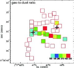
Figure 12.— Distribution of the box-averaged gas-to-dust ratio map. The black crosses show the positions of the nuclei defined by the peak positions of the Ks-band observation (Tateuchi et al., 2012). The open squares are regions which we cannot estimate the gas-to-dust ratio because of non-detection of the 340 GHz continuum emission.

6.4. Gas-to-Dust Ratio, $M_{\rm{H_{2}}}/M_{\rm{dust}}$

The gas-to-dust ratio, $M_{\rm{H_{2}}}$/$M_{\rm{dust}}$, provides an important measure of the relative abundance between gas and metallicity. The average $M_{\rm{H_{2}}}$/$M_{\rm{dust}}$ over the entire galaxy is often derived in single-dish work, and typical $M_{\rm{H_{2}}}$/$M_{\rm{dust}}$ is 200 – 300 for local U/LIRGs (Contini & Contini, 2003; Yao et al., 2003; Seaquist et al., 2004), and 15 – 231 in high-z sources (Solomon & Vanden Bout, 2005). Wilson et al. (2008) found $M_{\rm{H_{2}}}$/$M_{\rm{dust}}$ = 357 $\pm$ 95 from a sample of 13 U/LIRGs, including VV 114, observed at kpc resolution.

We use the gas and dust masses derived in §5.4 to investigate the distribution of $M_{\rm{H_{2}}}$/$M_{\rm{dust}}$ (Figure 12). The smallest value of (128 $\pm$ 16) $\left(\frac{\alpha_{\rm{CO}}}{0.8}\right)\left(\frac{0.9}{\kappa_{340}}\right)$ occurs in the eastern nucleus, which is similar to the Galactic value (100; Hildebrand, 1983), while higher values of (371 $\pm$ 118) $\left(\frac{\alpha_{\rm{CO}}}{0.8}\right)\left(\frac{0.9}{\kappa_{340}}\right)$ and (339 $\pm$ 60) $\left(\frac{\alpha_{\rm{CO}}}{0.8}\right)\left(\frac{0.9}{\kappa_{340}}\right)$ occur in the western nucleus and the overlap region, respectively. The clear differences between the two nuclei may suggest a local gradient in the metallicity. For the overlap region, cold dust associated with diffuse gas clouds cannot avoid the collision. This tends to increase the $M_{\rm{H_{2}}}$/$M_{\rm{dust}}$, because shocks destruct dust particles preferentially (Zhu et al., 2007). On the other hand, the low $M_{\rm{H_{2}}}$/$M_{\rm{dust}}$ in the eastern nucleus may be due to intense starbursts producing dust-rich environments.

6.5. Fractional Abundances of CS, CH₃OH, and CN

Table 15 shows the properties of the detected molecular lines which are not used in the RADEX calculations. Either the dense gas component of VV 114 has extreme variations in excitation among the molecular clumps in the filament (see §6.1), or there is widespread chemical differentiation across the filament. The fractional abundances [$N_{\rm{X}}/N_{\rm{H_{2}}}$] of the different astrochemical species provide evidence of varying chemical influences due to star formation, physical conditions, and dynamics across the galaxy disks. We use the H₂ column densities, derived from the RADEX calculations, which are 10^20.8, 10^21.1, and 10^21.1 cm^-2 at R18 (AGN), R21a (starburst), and R39a (overlap region), respectively. Column densities of each molecules are determined by equation (7) assuming an optically thin emission under LTE. The $T_{\rm{ex}}$ values determined from equation (3) are 38.7 $\pm$ 1.9 K, 58.8 $\pm$ 2.9 K, and 52.6 $\pm$ 2.6 K at R18, R21a, and R39a, respectively. The derived [$N_{\rm{X}}/N_{\rm{H_{2}}}$] are listed in Table 15.

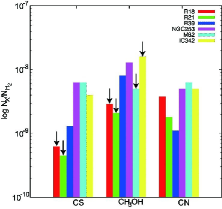
Figure 13.— Logarithmic fractional abundances relative to H₂ ([$X$]/[H₂]) of selected extragalactic sources compared to those of specific regions of VV 114, as presented in Table 15. The red, green, and blue columns show R18, R21a, and R39a, respectively. The pink, light blue, and yellow columns show NGC 253, M 82, and IC 342, respectively. Arrows represent upper limits.

In Figure 13, we show the fractional abundances for CS, CH₃OH, and CN in VV 114, and the same ratios for a sample of nearly galaxies, NGC 253, M82, and IC 342, taken from line surveys available in the literature (Henkel et al., 1988; Mauersberger et al., 1989; Huettemeister et al., 1997; Martín et al., 2006). M82 has a relatively old starburst at its core, with an average stellar population age of $\simeq$ 10 Myr (Konstantopoulos et al., 2009). This creates strong UV fields, therefore the PDR dominates its chemistry (Aladro et al., 2011). Figure 13 shows that R39a has higher CH₃OH abundance than M82, and small CS and CN abundances. A pure PDR similar to M82 may explain the molecular abundances we observe in R18.

The molecular abundances for the overlap region and NGC 253 share similar characteristics. NGC 253 is thought to be in an early stage of starburst evolution, and has young stellar populations in its nucleus ($\simeq$ 6 Myr; Fernández-Ontiveros et al., 2009). The chemistry in the nucleus of NGC 253 is dominated by large-scale shocks (Aladro et al., 2011), and we suggest that the overlap region of VV 114 is also dominated by shocks. The low $R_{\rm{HCN/HCO^{+}}}$ at the overlap region are further evidences for a shock dominated region (Krips et al., 2008).

6.6. Merger-driven Tidal Dwarf Galaxy Formation

Tidal dwarf galaxies (TDGs) are gas-rich irregular galaxies made out of stellar and gaseous material pulled out by tidal forces from the disks of the colliding parent galaxies into the intergalactic medium. They are found at the ends of long tails and host active star-forming regions (Braine et al., 2000). Hibbard et al. (2001) and Gao et al. (2001) found the HI gas mass of 4.1 $\times$ 10⁸ M_⊙ and the molecular gas mass of 4 $\times$ 10⁶ M_⊙ at the edge of the southern tail of NGC 4038/9.

We found an elevated $R_{3-2/1-0}$ (0.36 $\pm$ 0.01), SFR (0.10 $\pm$ 0.05 M_⊙ yr^-1), and $M_{\rm{H_{2}}}$ ($\sim$ 3.8 $\times$ 10⁷ $\left(\frac{\alpha_{\rm{CO}}}{0.8}\right)$ M_⊙) at the edge of the southern tidal arm (R38). The derived SFR and $M_{\rm{H_{2}}}$ of R38 are comparable to those of TDG candidates in other galaxies (Braine et al., 2001). The gas depletion time of (0.40 $\pm$ 0.22) $\left(\frac{\alpha_{\rm{CO}}}{0.8}\right)$ Gyr is shorter than the rest of the gas in the tidal arm ($>$ 0.5 $\left(\frac{\alpha_{\rm{CO}}}{0.8}\right)$ Gyr). According to the RADEX modeling, while the ranges of $T_{\rm{kin}}$ and $n_{\rm{H_{2}}}$ are not confined well, the best fitting values (35 K, 10^2.5 cm^-3) are slightly higher than those in the middle of the tidal arm, R36a and R37a (25 – 30 K, 10^2.0 – 10^2.2 cm^-3). We suggest that R38 is a forming tidal dwarf galaxy at the edge of the tidal arm of VV 114. Future high sensitivity optical and high resolution HI observations will allow us to constrain the star formation and the atomic gas properties of R38.

7. CONCLUSION

We investigate the physical conditions of the molecular gas in the mid-stage merger VV 114. We present high-resolution observations of molecular gas and dust continuum emission in this galaxy using ALMA band 3 and band 7. This study includes the first detection of extranuclear CH₃OH (2–1) emission in interacting galaxies. The results can be summarized as follows:

1. We find that the CO (1–0) and CO (3–2) lines show significantly extended structures (i.e., the northern and southern tidal arms), the central filament across the galaxy disks, and double-peaks in the overlap region, while the ¹³CO (1–0) line is only detected at the central filament. The filament is also identified by the strong CN (1_3/2 – 0_1/2), HCO⁺ (4–3), 110 GHz, and 340 GHz continuum emission.

2. Higher $R_{\rm{3-2/1-0}}$ (0.5 – 0.8) and $R_{\rm{12/13}}$ (20 – 50) are detected at the central filament. These higher ratios indicate that the central filament has highly excited (but not thermalized) molecular ISM, and the eastern nucleus is nearly thermalized when it is observed with a 800 pc beam.

3. The unresolved eastern nucleus has the highest $R_{\rm{HCN/HCO^{+}}}$ (1.34 $\pm$ 0.09), while the dense gas clumps near the eastern nucleus have significantly lower values ($\sim$ 0.5). The broad HCN (4–3) and HCO⁺ (4–3) ($\sim$ 290 km s^-1) emission lines seen in the unresolved eastern nucleus suggests an obscured AGN (see also paper I).

4. Radiative transfer analysis of the CO (1–0), CO (3–2), and ¹³CO (1–0) emission enables us to map physical parameters of the “diffuse” gas of an interacting LIRG with 800 pc scale for the first time. The analysis suggests that “diffuse” gas clouds in the filament have warmer/denser conditions than those in the galaxy disks. This is consistent with predictions from merger simulations. Our analysis also suggest that the [CO]/[¹³CO] is enhanced in the central filament. The extremely high [CO]/[¹³CO] values are more important than the moderately optically thick ¹²CO (1–0) emission to explain the high $R_{12/13}$ in VV 114.

5. Radiative transfer analysis of the HCN (4–3), HCO⁺ (4–3), and ¹²CO (3–2) allow us to compare the dense gas clouds around AGN, starburst activities, and the overlap region. These results show that dense gas clouds around AGN have $n_{\rm{H_{2}}}$ = 10^5.0 – 10^5.4 cm^-3 and $T_{\rm{kin}}$ $>$ 100 K with [HCN]/[HCO⁺] $>$ 5, while gas clumps around starburst activities show $n_{\rm{H_{2}}}$ = 10^5.6 – 10^5.9 cm^-3 and $T_{\rm{kin}}$ = 40 –100 K with [HCN]/[HCO⁺] $<$ 4. In addition, the analysis shows that the overlap region has $n_{\rm{H_{2}}}$ = 10^5.0 – 10^5.6 cm^-3 and $T_{\rm{kin}}$ = 5 – 90 K with [HCN]/[HCO⁺] = 1 – 9.

6. The spatially resolved Kennicutt-Schmidt law in VV 114 clearly connects the “starburst” sequence with the “normal disk” sequence. Most of the data points near the “starburst” sequence are found in the nuclei and the overlap region, whereas the data points near the “normal disk” sequence are found in the tidal arms. We also find the $R_{\rm{3-2/1-0}}$ and $R_{\rm{12/13}}$ are well correlated with the $\Sigma_{\rm{SFR}}$.

7. The $M_{\rm{H_{2}}}$/$M_{\rm{dust}}$ of (128 $\pm$ 16) $\left(\frac{\alpha_{\rm{CO}}}{0.8}\right)\left(\frac{0.9}{\kappa_{340}}\right)$ in the eastern nucleus of VV 114 is comparable to the Galactic value, but it is a factor of two higher than that in the overlap region of (339 $\pm$ 60) $\left(\frac{\alpha_{\rm{CO}}}{0.8}\right)\left(\frac{0.9}{\kappa_{340}}\right)$. Since the 340 GHz emission is spatially correlated with dense gas tracers, the cold dust in VV 114 appears to be closely related to the dense molecular component in the filament. The lowest $M_{\rm{H_{2}}}$/$M_{\rm{dust}}$ in the eastern nucleus may be due to the dusty starburst.

8. Comparing the CS, CN, and CH₃OH emission with other galaxies, we suggest that the overlap region is dominated by large-scale shocks similar to the nucleus of NGC 253. From the abundance analysis and distribution of the line ratios, we postulate that the HCN-rich AGN, the HCO⁺-rich starbursts, and the CH₃OH-rich overlap region are important drivers of the molecular chemistry of VV 114.

9. We find a region with relatively high excitation ($\simeq$ 35 K, $\simeq$ 10^2.5 cm^-3) and star formation (SFR = 0.10 $\pm$ 0.05 M_⊙ yr^-1) at the edge of the southern tail. This region has a shorter $\tau_{\rm{gas}}$ of (0.40 $\pm$ 0.22) $\left(\frac{\alpha_{\rm{CO}}}{0.8}\right)$ Gyr than the rest of the southern tail ($>$ 1.35 $\left(\frac{\alpha_{\rm{CO}}}{0.8}\right)$ Gyr), and we suggest that it is a forming tidal dwarf galaxy.

Table 1Log of ALMA Observations

UT date	Spectral windows			Configuration			$T_{\rm{sys}}$	MRS	Amplitude caibrator	$T_{\rm{obs}}$
	LSB	USB		$N_{\rm{ant}}$	Array	$L_{\rm{baseline}}$
	[GHz]	[GHz]				[m]	[K]	[arcsec.]		[min.]
(1)	(2)	(3)		(4)	(5)	(6)	(7)	(8)	(9)	(10)
2011 Nov 6	101.5, 103.5	114.0, 115.1		16	CMP	18 - 196	065 - 089	18	Uranus	41
2012 May 4	101.5, 103.5	114.0, 115.1		15	EXT	39 - 402	048 - 062	08	Neptune	40
2012 Mar 27	097.5, 099.5	110.2, 111.5		17	EXT	18 - 401	054 - 073	19	Neptune	22
2012 Jul 2	097.5, 099.5	110.2, 111.5		20	EXT	16 - 402	071 - 117	21	Neptune	39
2012 Nov 5	331.1, 333.0	343.5, 345.3		14	CMP	12 - 135	125 - 172	09	Uranus	66
2012 Nov 5	331.1, 333.0	343.5, 345.3		14	CMP	12 - 135	108 - 155	09	Uranus	67
2012 Nov 5	331.1, 333.0	343.5, 345.3		14	CMP	12 - 135	124 - 175	09	Callisto	67
2012 Jun 1	342.0, 344.0	354.5, 356.0		18	EXT	15 - 402	150 - 213	07	Uranus	78
2012 Jun 2	342.0, 344.0	354.5, 356.0		20	EXT	15 - 402	108 - 160	07	Uranus	80
2012 Jun 3	342.0, 344.0	354.5, 356.0		20	EXT	15 - 402	103 - 130	07	Uranus	45

Note. — Column 2 and 3: Central frequencies of the spectral windows (spw). All spw have the frequency coverage of 1.875 GHz. Column 4: Number of available antennas. Column 5: ALMA antenna configuration. CMP is the compact configuration and EXT is the extended configuration. Column 6: Range of projected length of baselines for VV 114. Column 7: DSB system temperature toward VV 114. Column 8: Maximum recoverable scale (MRS) of the configuration. This is defined by $\sim$ 0.6 $\lambda$/(minimum $L_{\rm{baseline}}$). Column 9: Observed calibrators for amplitude correction. Column 10: Total integration time on the galaxy.

Table 2ALMA Observational Properties

Emission	Band	$\nu_{\rm{rest}}$	Beam size	P.A.	$\Delta$V	Noise rms
		[GHz]	[arcsecond]	[deg]	[km s-1]	[mJy beam-1]	[mK]
(1)	(2)	(3)	(4)	(5)	(6)	(7)	(8)
CH3OH (2k–1k)	3	96.74	2.03 $\times$ 1.34	85.7	30	1.0	46
CS (2–1)	3	97.98	2.01 $\times$ 1.37	83.6	30	0.9	40
13CO (1–0)	3	110.20	1.77 $\times$ 1.20	85.8	30	1.0	46
CN (11/2–01/2)	3	113.14	1.97 $\times$ 1.27	$-$85.8	30	1.0	37
CN (13/2–01/2)	3	113.49	1.98 $\times$ 1.29	$-$84.7	30	1.1	39
CO (1–0)	3	115.27	1.97 $\times$ 1.35	82.3	10	2.3	76
CS (7–6)	7	342.88	0.47 $\times$ 0.39	54.2	30	0.7	38
CO (3–2)	7	345.80	1.64 $\times$ 1.17	112.6	10	2.1	11
HCN (4–3)	7	354.51	0.46 $\times$ 0.38	51.5	30	0.8	42
HCO+ (4–3)	7	356.73	0.45 $\times$ 0.37	53.4	30	0.9	50
Continuum	3	110	1.89 $\times$ 1.28	81.8	$\cdots$	0.05	2.1
Continuum	7	340	1.33 $\times$ 1.12	119.6	$\cdots$	0.11	0.8
Continuum	7	340	0.45 $\times$ 0.38	56.2	$\cdots$	0.07	4.3

Note. — Column 1: Identified emission. Column 2: Band which includes the molecular line and continuum emission. Column 3: Rest frequency of the line or mean frequency of the continuum. Column 4: Major and minor axes (FWHM) of the synthesized beam. Column 5: Position angle of the synthesized beam. Column 6: Velocity resolution of our binning images. Column 7 and 8: Noise rms intensity in the data which have velocity resolutions shown in Column 6. The noise in Column 8 is in Rayleigh-Jeans brightness temperature.

Table 3Radio Continuum Flux of VV 114

ID	$S_{8.44}$	$S_{110}$	$S_{340}$
	[mJy]	[mJy]	[mJy]
(1)	(2)	(3)	(4)
R7	0.62 $\pm$ 0.08	$<$ 0.18	0.58 $\pm$ 0.14
R8	0.70 $\pm$ 0.08	$<$ 0.18	$<$ 0.42
R9	0.82 $\pm$ 0.08	0.21 $\pm$ 0.06	$<$ 0.42
R10	0.81 $\pm$ 0.08	0.20 $\pm$ 0.06	$<$ 0.42
R11	0.92 $\pm$ 0.08	$<$ 0.18	$<$ 0.42
R17	0.42 $\pm$ 0.08	$<$ 0.18	$<$ 0.42
R18†	3.37 $\pm$ 0.08	1.48 $\pm$ 0.06	5.17 $\pm$ 0.14
R19	2.40 $\pm$ 0.08	1.03 $\pm$ 0.06	3.03 $\pm$ 0.14
R20	1.14 $\pm$ 0.08	0.54 $\pm$ 0.06	2.41 $\pm$ 0.14
R21††	5.00 $\pm$ 0.08	1.86 $\pm$ 0.06	8.20 $\pm$ 0.14
R22	1.85 $\pm$ 0.08	0.81 $\pm$ 0.06	4.37 $\pm$ 0.14
R23	1.34 $\pm$ 0.08	0.50 $\pm$ 0.06	3.55 $\pm$ 0.14
R24	0.67 $\pm$ 0.08	$<$ 0.18	1.19 $\pm$ 0.14
R25	1.07 $\pm$ 0.08	0.39 $\pm$ 0.06	3.01 $\pm$ 0.14
R26	0.81 $\pm$ 0.08	0.33 $\pm$ 0.06	1.73 $\pm$ 0.14
R27	1.29 $\pm$ 0.08	0.41 $\pm$ 0.06	1.40 $\pm$ 0.14
R28	0.81 $\pm$ 0.08	0.21 $\pm$ 0.06	0.76 $\pm$ 0.14
R29	0.35 $\pm$ 0.08	$<$ 0.18	0.71 $\pm$ 0.14
R30	$<$ 0.24	$<$ 0.18	0.70 $\pm$ 0.14
R39†††	1.18 $\pm$ 0.08	0.21 $\pm$ 0.06	3.35 $\pm$ 0.14

Note. — Column 2: 8.44 GHz continuum flux (Condon et al., 1991). Column 3: 110 GHz continuum flux obtained by ALMA/band 3. Column 4: 340 GHz continuum flux obtained by ALMA/band 7.; We only show the statistical error in this table. The systematic error of absolute flux calibration is estimated to be $\sim$ 5% in band 3 and $\sim$ 10% in band 7. †represents boxes contained the obscured AGN defined by paper I. ††represents boxes contained the nuclear starbursts defined by paper I. †††represents boxes at the overlap region.

Table 4CO (1–0), ¹³CO (1–0), and ¹²CO (3–2) Integrated Intensities

ID	12CO (1–0)	12CO (3–2)	13CO (1–0)	$R_{3-2/1-0}$	$R_{12/13}$
	[Jy km s-1]	[Jy km s-1]	[Jy km s-1]
(1)	(2)	(3)	(4)	(5)	(6)
R1	2.12 $\pm$ 0.06	5.92 $\pm$ 0.08	$\cdots$	0.31 $\pm$ 0.01	$\cdots$
R2	1.41 $\pm$ 0.05	7.47 $\pm$ 0.06	0.29 $\pm$ 0.02	0.59 $\pm$ 0.02	4 $\pm$ 1
R3	3.62 $\pm$ 0.09	5.45 $\pm$ 0.09	$\cdots$	0.17 $\pm$ 0.01	$\cdots$
R4	3.54 $\pm$ 0.08	8.69 $\pm$ 0.10	0.25 $\pm$ 0.04	0.27 $\pm$ 0.01	13 $\pm$ 2
R5	3.46 $\pm$ 0.08	9.16 $\pm$ 0.09	0.40 $\pm$ 0.03	0.29 $\pm$ 0.01	7 $\pm$ 1
R6	3.66 $\pm$ 0.10	10.71 $\pm$ 0.11	$\cdots$	0.33 $\pm$ 0.01	$\cdots$
R7	5.26 $\pm$ 0.10	19.64 $\pm$ 0.12	0.40 $\pm$ 0.03	0.41 $\pm$ 0.01	12 $\pm$ 1
R8	3.71 $\pm$ 0.09	13.44 $\pm$ 0.12	0.38 $\pm$ 0.03	0.40 $\pm$ 0.01	8 $\pm$ 1
R9	9.59 $\pm$ 0.11	33.88 $\pm$ 0.12	0.43 $\pm$ 0.04	0.39 $\pm$ 0.01	20 $\pm$ 2
R10	12.69 $\pm$ 0.11	47.74 $\pm$ 0.12	0.37 $\pm$ 0.05	0.42 $\pm$ 0.01	32 $\pm$ 4
R11	16.26 $\pm$ 0.13	58.93 $\pm$ 0.14	0.49 $\pm$ 0.04	0.40 $\pm$ 0.01	30 $\pm$ 3
R12	4.61 $\pm$ 0.10	13.53 $\pm$ 0.10	$\cdots$	0.33 $\pm$ 0.01	$\cdots$
R13	5.22 $\pm$ 0.10	16.02 $\pm$ 0.11	0.38 $\pm$ 0.05	0.34 $\pm$ 0.01	12 $\pm$ 2
R14	4.70 $\pm$ 0.09	12.22 $\pm$ 0.09	0.35 $\pm$ 0.03	0.29 $\pm$ 0.01	12 $\pm$ 1
R15	5.03 $\pm$ 0.09	10.62 $\pm$ 0.09	0.35 $\pm$ 0.03	0.23 $\pm$ 0.01	13 $\pm$ 1
R16	5.59 $\pm$ 0.09	11.23 $\pm$ 0.08	0.38 $\pm$ 0.02	0.22 $\pm$ 0.01	14 $\pm$ 1
R17	6.44 $\pm$ 0.10	14.33 $\pm$ 0.11	0.38 $\pm$ 0.05	0.25 $\pm$ 0.01	15 $\pm$ 2
R18†	16.54 $\pm$ 0.13	106.39 $\pm$ 0.15	0.60 $\pm$ 0.05	0.71 $\pm$ 0.01	25 $\pm$ 2
R19	11.09 $\pm$ 0.12	54.98 $\pm$ 0.14	0.60 $\pm$ 0.05	0.55 $\pm$ 0.01	17 $\pm$ 2
R20	18.33 $\pm$ 0.13	93.14 $\pm$ 0.14	0.64 $\pm$ 0.06	0.56 $\pm$ 0.01	26 $\pm$ 2
R21††	33.04 $\pm$ 0.15	225.47 $\pm$ 0.16	1.09 $\pm$ 0.07	0.76 $\pm$ 0.01	28 $\pm$ 2
R22	28.67 $\pm$ 0.15	162.41 $\pm$ 0.16	0.90 $\pm$ 0.07	0.63 $\pm$ 0.01	29 $\pm$ 2
R23	33.65 $\pm$ 0.16	177.02 $\pm$ 0.17	0.95 $\pm$ 0.07	0.58 $\pm$ 0.01	32 $\pm$ 2
R24	16.12 $\pm$ 0.14	68.28 $\pm$ 0.15	0.48 $\pm$ 0.07	0.47 $\pm$ 0.01	31 $\pm$ 4
R25	25.23 $\pm$ 0.16	138.20 $\pm$ 0.16	0.86 $\pm$ 0.06	0.61 $\pm$ 0.01	27 $\pm$ 2
R26	20.44 $\pm$ 0.14	97.56 $\pm$ 0.15	0.69 $\pm$ 0.06	0.53 $\pm$ 0.01	27 $\pm$ 3
R27	12.45 $\pm$ 0.12	67.10 $\pm$ 0.13	0.54 $\pm$ 0.06	0.60 $\pm$ 0.01	21 $\pm$ 2
R28	5.78 $\pm$ 0.10	36.14 $\pm$ 0.14	0.35 $\pm$ 0.03	0.69 $\pm$ 0.01	15 $\pm$ 1
R29	$\cdots$	$\cdots$	$\cdots$	$\cdots$	$\cdots$
R30	6.39 $\pm$ 0.12	30.50 $\pm$ 0.12	0.28 $\pm$ 0.03	0.53 $\pm$ 0.01	21 $\pm$ 3
R31	4.93 $\pm$ 0.11	19.03 $\pm$ 0.13	0.30 $\pm$ 0.04	0.43 $\pm$ 0.01	15 $\pm$ 2
R32	2.34 $\pm$ 0.05	7.34 $\pm$ 0.08	0.21 $\pm$ 0.02	0.35 $\pm$ 0.01	10 $\pm$ 1
R33	1.44 $\pm$ 0.05	2.03 $\pm$ 0.05	$\cdots$	0.16 $\pm$ 0.01	$\cdots$
R34	2.81 $\pm$ 0.08	11.65 $\pm$ 0.10	0.32 $\pm$ 0.03	0.46 $\pm$ 0.01	8 $\pm$ 1
R35	5.36 $\pm$ 0.09	9.40 $\pm$ 0.09	0.30 $\pm$ 0.03	0.19 $\pm$ 0.01	16 $\pm$ 2
R36	5.55 $\pm$ 0.12	17.95 $\pm$ 0.14	0.31 $\pm$ 0.02	0.36 $\pm$ 0.01	17 $\pm$ 1
R37	4.84 $\pm$ 0.11	8.65 $\pm$ 0.11	0.31 $\pm$ 0.03	0.20 $\pm$ 0.01	14 $\pm$ 2
R38	2.66 $\pm$ 0.07	8.51 $\pm$ 0.09	0.33 $\pm$ 0.02	0.36 $\pm$ 0.01	7 $\pm$ 1
R39†††	27.54 $\pm$ 0.15	155.31 $\pm$ 0.15	0.97 $\pm$ 0.06	0.63 $\pm$ 0.01	26 $\pm$ 2

Note. — Column 1: These numbers are labeled at the ratio map of Figure 7. Column 2: Integrated ¹²CO (1–0) intensity at an emission region. Column 3: Integrated ¹²CO (3–2) intensity at an emission region. Column 4: Integrated ¹³CO (3–2) intensity at an emission region. Column 5: The ¹²CO (3–2)/CO (1–0) integrated intensity ratio. Column 6: The ¹²CO (1–0)/¹³CO (1–0) integrated intensity ratio.; We only show the statistical error in this table. The systematic error of absolute flux calibration is estimated to be $\sim$ 5% in band 3 and $\sim$ 10% in band 7. †represents boxes contained the obscured AGN defined by paper I. ††represents boxes contained the nuclear starbursts defined by paper I. †††represents boxes at the overlap region.

Table 5HCN (4–3) and HCO⁺ (4–3) Integrated Intensities

ID	HCN (4–3)	HCO+ (4–3)	$R_{\rm{HCN/HCO^{+}}}$
	[Jy km s-1]	[Jy km s-1]
(1)	(2)	(3)	(4)
S0†	1.34 $\pm$ 0.09	0.88$\pm$ 0.10	1.52 $\pm$ 0.20
S1	0.11 $\pm$ 0.03	0.34$\pm$ 0.06	0.34 $\pm$ 0.10
S2	$<$ 0.05	0.12$\pm$ 0.06	$<$ 0.43
S3††	0.49 $\pm$ 0.07	1.05$\pm$ 0.08	0.46 $\pm$ 0.07
S4	0.13 $\pm$ 0.06	0.63$\pm$ 0.08	0.20 $\pm$ 0.09
S5††	0.81 $\pm$ 0.07	2.36$\pm$ 0.09	0.34 $\pm$ 0.03
S6	0.40 $\pm$ 0.07	0.92$\pm$ 0.08	0.43 $\pm$ 0.09
S7	0.19 $\pm$ 0.07	0.42$\pm$ 0.08	0.45 $\pm$ 0.18
S8	0.06 $\pm$ 0.04	0.14$\pm$ 0.06	0.44 $\pm$ 0.31
S9	0.07 $\pm$ 0.05	0.13$\pm$ 0.06	0.54 $\pm$ 0.46
S10	$<$ 0.04	0.28$\pm$ 0.07	$<$ 0.14
S11†††	$<$ 0.05	0.15$\pm$ 0.06	$<$ 0.33
S12†††	$<$ 0.04	0.32$\pm$ 0.07	$<$ 0.12
S13	$<$ 0.04	0.17$\pm$ 0.06	$<$ 0.24
S14	$<$ 0.05	0.19$\pm$ 0.07	$<$ 0.26

Note. — Column 1: These numbers are labeled at the ratio map of Figure 7. Column 2: Integrated HCN (4–3) intensity at an emission region. Column 3: Integrated HCO⁺ (4–3) intensity at an emission region. Column 4: The HCN (4–3)/HCO⁺ (4–3) integrated intensity ratio.; We only show the statistical error in this table. The systematic error of absolute flux calibration is estimated to be $\sim$ 5% in band 3 and $\sim$ 10% in band 7. †represents boxes contained the obscured AGN defined by paper I. ††represents boxes contained the nuclear starbursts defined by paper I. †††represents boxes at the overlap region.

Table 6Peak Brightness Temperature of ¹²CO (1–0), ¹³CO (1–0), and ¹²CO (3–2) Emission

ID	Peak $T_{\rm{b,CO~{}(1-0)}}$	Peak $T_{\rm{b,CO~{}(3-2)}}$	Peak $T_{\rm{b,^{13}CO~{}(1-0)}}$	Peak $R_{3-2/1-0}$	Peak $R_{12/13}$
	[K]	[K]	[K]
(1)	(2)	(3)	(4)	(5)	(6)
R1	0.40 $\pm$ 0.07	0.13 $\pm$ 0.01	$<$ 0.09	0.32 $\pm$ 0.07	$>$ 4
R2	0.69 $\pm$ 0.07	0.25 $\pm$ 0.01	$<$ 0.09	0.37 $\pm$ 0.04	$>$ 8
R3	0.61 $\pm$ 0.07	0.07 $\pm$ 0.01	$<$ 0.09	0.12 $\pm$ 0.02	$>$ 7
R4	0.98 $\pm$ 0.07	0.30 $\pm$ 0.01	$<$ 0.09	0.30 $\pm$ 0.02	$>$ 11
R5	1.19 $\pm$ 0.07	0.42 $\pm$ 0.01	0.06 $\pm$ 0.03	0.35 $\pm$ 0.02	20 $\pm$ 2
R6	0.87 $\pm$ 0.07	0.21 $\pm$ 0.01	$<$ 0.09	0.24 $\pm$ 0.02	$>$ 10
R7a	1.34 $\pm$ 0.07	0.32 $\pm$ 0.01	$<$ 0.09	0.24 $\pm$ 0.01	$>$ 15
R7b	0.45 $\pm$ 0.07	0.36 $\pm$ 0.01	0.06 $\pm$ 0.03	0.79 $\pm$ 0.12	7 $\pm$ 1
R8a	0.21 $\pm$ 0.07	$<$ 0.03	$<$ 0.09	$>$ 0.14	$>$ 2
R8b	0.96 $\pm$ 0.07	0.24 $\pm$ 0.01	0.08 $\pm$ 0.03	0.25 $\pm$ 0.02	11 $\pm$ 1
R9a	0.40 $\pm$ 0.07	0.12 $\pm$ 0.01	$<$ 0.09	0.30 $\pm$ 0.06	$>$ 4
R9b	2.60 $\pm$ 0.07	0.99 $\pm$ 0.01	0.08 $\pm$ 0.03	0.38 $\pm$ 0.01	33 $\pm$ 2
R10a	0.80 $\pm$ 0.07	0.24 $\pm$ 0.01	0.05 $\pm$ 0.03	0.30 $\pm$ 0.03	17 $\pm$ 2
R10b	2.81 $\pm$ 0.07	1.27 $\pm$ 0.01	0.09 $\pm$ 0.03	0.45 $\pm$ 0.01	30 $\pm$ 1
R11a	2.11 $\pm$ 0.07	0.82 $\pm$ 0.01	0.12 $\pm$ 0.03	0.39 $\pm$ 0.01	18 $\pm$ 1
R11b	3.34 $\pm$ 0.07	1.36 $\pm$ 0.01	0.04 $\pm$ 0.03	0.41 $\pm$ 0.01	89 $\pm$ 7
R12a	0.55 $\pm$ 0.07	0.23 $\pm$ 0.01	$<$ 0.09	0.41 $\pm$ 0.06	$>$ 6
R12b	1.30 $\pm$ 0.07	0.41 $\pm$ 0.01	$<$ 0.09	0.32 $\pm$ 0.02	$>$ 14
R13a	1.12 $\pm$ 0.07	0.34 $\pm$ 0.01	0.06 $\pm$ 0.03	0.30 $\pm$ 0.02	18 $\pm$ 1
R13b	0.67 $\pm$ 0.07	0.30 $\pm$ 0.01	$<$ 0.09	0.45 $\pm$ 0.05	$>$ 7
R14	1.61 $\pm$ 0.07	0.39 $\pm$ 0.01	0.08 $\pm$ 0.03	0.24 $\pm$ 0.01	20 $\pm$ 1
R15	1.77 $\pm$ 0.07	0.42 $\pm$ 0.01	0.08 $\pm$ 0.03	0.24 $\pm$ 0.01	22 $\pm$ 1
R16	1.38 $\pm$ 0.07	0.33 $\pm$ 0.01	0.12 $\pm$ 0.03	0.24 $\pm$ 0.01	12 $\pm$ 1
R17	1.64 $\pm$ 0.07	0.35 $\pm$ 0.01	0.05 $\pm$ 0.03	0.21 $\pm$ 0.01	36 $\pm$ 3
R18†	3.52 $\pm$ 0.07	1.79 $\pm$ 0.01	0.14 $\pm$ 0.03	0.51 $\pm$ 0.01	25 $\pm$ 1
R19a	1.01 $\pm$ 0.07	0.54 $\pm$ 0.01	0.09 $\pm$ 0.03	0.54 $\pm$ 0.04	11 $\pm$ 1
R19b	1.99 $\pm$ 0.07	0.98 $\pm$ 0.01	0.09 $\pm$ 0.03	0.49 $\pm$ 0.02	23 $\pm$ 1
R20a	3.33 $\pm$ 0.07	1.99 $\pm$ 0.01	0.11 $\pm$ 0.03	0.60 $\pm$ 0.01	30 $\pm$ 1
R20b	1.13 $\pm$ 0.07	0.67 $\pm$ 0.01	$<$ 0.09	0.59 $\pm$ 0.04	$>$ 13
R21a††	5.53 $\pm$ 0.07	4.49 $\pm$ 0.01	0.23 $\pm$ 0.03	0.81 $\pm$ 0.01	24 $\pm$ 1
R21b††	1.22 $\pm$ 0.07	0.95 $\pm$ 0.01	$<$ 0.09	0.78 $\pm$ 0.05	$>$ 14
R21c††	0.40 $\pm$ 0.07	0.72 $\pm$ 0.01	$<$ 0.09	1.80 $\pm$ 0.05	$>$ 4
R22a	3.60 $\pm$ 0.07	1.93 $\pm$ 0.01	0.12 $\pm$ 0.03	0.54 $\pm$ 0.01	29 $\pm$ 1
R22b	3.83 $\pm$ 0.07	2.61 $\pm$ 0.01	0.16 $\pm$ 0.03	0.68 $\pm$ 0.01	24 $\pm$ 1
R23a	4.17 $\pm$ 0.07	2.56 $\pm$ 0.01	0.15 $\pm$ 0.03	0.61 $\pm$ 0.01	28 $\pm$ 1
R23b	3.39 $\pm$ 0.07	1.87 $\pm$ 0.01	0.12 $\pm$ 0.03	0.55 $\pm$ 0.01	28 $\pm$ 1
R24a	1.23 $\pm$ 0.07	0.46 $\pm$ 0.01	0.05 $\pm$ 0.03	0.37 $\pm$ 0.02	23 $\pm$ 2
R24b	1.60 $\pm$ 0.07	0.96 $\pm$ 0.01	0.06 $\pm$ 0.03	0.60 $\pm$ 0.03	28 $\pm$ 2
R24c	1.78 $\pm$ 0.07	0.58 $\pm$ 0.01	0.06 $\pm$ 0.03	0.32 $\pm$ 0.01	32 $\pm$ 2
R25a	4.89 $\pm$ 0.07	3.18 $\pm$ 0.01	0.23 $\pm$ 0.03	0.65 $\pm$ 0.01	21 $\pm$ 1
R25b	1.77 $\pm$ 0.07	0.59 $\pm$ 0.01	0.06 $\pm$ 0.03	0.33 $\pm$ 0.01	31 $\pm$ 2
R26a	4.49 $\pm$ 0.07	2.57 $\pm$ 0.01	0.14 $\pm$ 0.03	0.57 $\pm$ 0.01	33 $\pm$ 1
R26b	1.07 $\pm$ 0.07	0.31 $\pm$ 0.01	0.07 $\pm$ 0.03	0.29 $\pm$ 0.02	15 $\pm$ 1
R27a	1.96 $\pm$ 0.07	1.31$\pm$ 0.01	0.04 $\pm$ 0.03	0.67 $\pm$ 0.02	47 $\pm$ 4
R27b	1.53 $\pm$ 0.07	0.75 $\pm$ 0.01	0.13 $\pm$ 0.03	0.49 $\pm$ 0.02	12 $\pm$ 1
R28a	0.76 $\pm$ 0.07	0.37 $\pm$ 0.01	0.05 $\pm$ 0.03	0.48 $\pm$ 0.05	16 $\pm$ 2
R28b	0.86 $\pm$ 0.07	0.54 $\pm$ 0.01	$<$ 0.09	0.62 $\pm$ 0.05	$>$ 10
R29	$<$ 0.21	$<$ 0.03	$<$ 0.09	$\cdots$	$\cdots$
R30a	0.77 $\pm$ 0.07	0.39 $\pm$ 0.01	$<$ 0.09	0.51 $\pm$ 0.05	$>$ 9
R30b	1.39 $\pm$ 0.07	0.69 $\pm$ 0.01	$<$ 0.09	0.50 $\pm$ 0.03	$>$ 15
R31a	0.72 $\pm$ 0.07	0.33 $\pm$ 0.01	0.06 $\pm$ 0.03	0.46 $\pm$ 0.03	13 $\pm$ 1
R31b	0.55 $\pm$ 0.07	0.24 $\pm$ 0.01	$<$ 0.09	0.44 $\pm$ 0.06	$>$ 6
R32	0.55 $\pm$ 0.07	0.29 $\pm$ 0.01	$<$ 0.09	0.52 $\pm$ 0.07	$>$ 6
R33	0.35 $\pm$ 0.07	0.14 $\pm$ 0.01	$<$ 0.09	0.41 $\pm$ 0.09	$>$ 4
R34	0.83 $\pm$ 0.07	0.37 $\pm$ 0.01	0.05 $\pm$ 0.03	0.45 $\pm$ 0.04	18 $\pm$ 2
R35	1.42 $\pm$ 0.07	0.30 $\pm$ 0.01	$<$ 0.09	0.21 $\pm$ 0.01	$>$ 16
R36a	0.65 $\pm$ 0.07	0.24 $\pm$ 0.01	0.07 $\pm$ 0.03	0.37 $\pm$ 0.04	9 $\pm$ 1
R36b	0.47 $\pm$ 0.07	0.22 $\pm$ 0.01	$<$ 0.09	0.47 $\pm$ 0.07	$>$ 5
R37a	0.79 $\pm$ 0.07	0.15 $\pm$ 0.01	0.06 $\pm$ 0.03	0.19 $\pm$ 0.02	14 $\pm$ 1
R37b	0.71 $\pm$ 0.07	0.18 $\pm$ 0.01	$<$ 0.09	0.26 $\pm$ 0.03	$>$ 8
R38	0.38 $\pm$ 0.07	0.16 $\pm$ 0.01	0.04 $\pm$ 0.03	0.42 $\pm$ 0.08	9 $\pm$ 2
R39a†††	4.91 $\pm$ 0.07	3.15 $\pm$ 0.01	0.24 $\pm$ 0.03	0.64 $\pm$ 0.01	21 $\pm$ 1
R39b†††	1.96 $\pm$ 0.07	0.81 $\pm$ 0.01	0.06 $\pm$ 0.03	0.41 $\pm$ 0.02	31 $\pm$ 2

Note. — Column 1: These numbers are labeled at the ratio map of Figure 7. Column 2: Peak ¹²CO (1–0) brightness temperature at an emission region. Column 3: Peak ¹²CO (3–2) brightness temperature at an emission region. Column 4: Peak ¹³CO (3–2) brightness temperature at an emission region. Column 5: The ¹²CO (3–2)/CO (1–0) brightness temperature ratio. Column 6: The ¹²CO (1–0)/¹³CO (1–0) brightness temperature ratio.; We only show the statistical error in this table. The systematic error of absolute flux calibration is estimated to be $\sim$ 5% in band 3 and $\sim$ 10% in band 7. †represents boxes contained the obscured AGN defined by paper I. ††represents boxes contained the nuclear starbursts defined by paper I. †††represents boxes at the overlap region.

Table 7Peak Brightness Temperature of HCN (4–3) and HCO⁺ (4–3)

ID	$T_{\rm{b,HCN~{}(4-3)}}$	$T_{\rm{b,HCO^{+}(4-3)}}$	$R_{\rm{HCN/HCO^{+}}}$
	[K]	[K]
(1)	(2)	(3)	(4)
S0†	0.32 $\pm$ 0.05	0.27 $\pm$ 0.05	1.18 $\pm$ 0.29
S1	$<$ 0.15	0.20 $\pm$ 0.05	$<$ 0.75
S2	$<$ 0.15	0.16 $\pm$ 0.05	$<$ 0.94
S3††	0.20 $\pm$ 0.05	0.65 $\pm$ 0.05	0.31 $\pm$ 0.08
S4	0.10 $\pm$ 0.05	0.51 $\pm$ 0.05	0.19 $\pm$ 0.10
S5††	0.32 $\pm$ 0.05	0.91 $\pm$ 0.05	0.35 $\pm$ 0.06
S6	0.14 $\pm$ 0.05	0.55 $\pm$ 0.05	0.26 $\pm$ 0.09
S7	$<$ 0.15	0.24 $\pm$ 0.05	$<$ 0.63
S8	$<$ 0.15	0.14 $\pm$ 0.05	$<$ 1.07
S9	$<$ 0.15	0.17 $\pm$ 0.05	$<$ 0.88
S10	0.10 $\pm$ 0.05	0.17 $\pm$ 0.05	0.60 $\pm$ 0.34
S11†††	$<$ 0.15	0.18 $\pm$ 0.05	$<$ 0.83
S12†††	$<$ 0.15	0.24 $\pm$ 0.05	$<$ 0.63
S13	$<$ 0.15	0.20 $\pm$ 0.05	$<$ 0.75
S14	$<$ 0.15	0.23 $\pm$ 0.05	$<$ 0.65

Note. — Column 1: These numbers are labeled at the ratio map of Figure 7. Column 2: Peak HCN (4–3) brightness temperature at an emission region. Column 3: Peak HCO⁺ (4–3) brightness temperature at an emission region. Column 4: The HCN (4–3)/HCO⁺ (4–3) brightness temperature ratio.; We only show the statistical error in this table. The systematic error of absolute flux calibration is estimated to be $\sim$ 5% in band 3 and $\sim$ 10% in band 7. †represents boxes contained the obscured AGN defined by paper I. ††represents boxes contained the nuclear starbursts defined by paper I. †††represents boxes at the overlap region.

Table 8Peak Brightness Temperature of ¹²CO (3–2), HCN (4–3), and HCO⁺ (4–3)

ID	Peak $T_{\rm{b,CO~{}(3-2)}}$	Peak $T_{\rm{b,HCN~{}(4-3)}}$	Peak $T_{\rm{b,HCO^{+}(4-3)}}$	Peak $R_{\rm{HCO^{+}/CO}}$	Peak $R_{\rm{HCN/HCO^{+}}}$
	[K]	[K]	[K]
(1)	(2)	(3)	(4)	(5)	(6)
E0†	2.94 $\pm$ 0.04	0.06 $\pm$ 0.01	0.04 $\pm$ 0.01	0.014 $\pm$ 0.004	1.55 $\pm$ 0.49
E1††	5.82 $\pm$ 0.04	0.11 $\pm$ 0.01	0.32 $\pm$ 0.01	0.056 $\pm$ 0.002	0.36 $\pm$ 0.03
E2†††	4.71 $\pm$ 0.04	0.04 $\pm$ 0.01	0.08 $\pm$ 0.01	0.017 $\pm$ 0.002	0.52 $\pm$ 0.14

Note. — Column 1: These numbers are regions where were convolved to the 1$\farcs$2 $\times$ 1$\farcs$0 resolution (P.A. = 119 deg.). Column 2: Peak ¹²CO (3–2) brightness temperature at an emission region. Column 3: Peak HCN (4–3) brightness temperature at an emission region. Column 4: Peak HCO⁺ (4–3) brightness temperature at an emission region. Column 5: The HCO⁺ (4–3)/CO (3–2) brightness temperature ratio. Column 6: The HCN (4–3)/HCO⁺ (4–3) brightness temperature ratio.; We only show the statistical error in this table. The systematic error of absolute flux calibration is estimated to be $\sim$ 5% in band 3 and $\sim$ 10% in band 7. †represents boxes contained the obscured AGN defined by paper I. ††represents boxes contained the nuclear starbursts defined by paper I. †††represents boxes at the overlap region.

Table 9Parameters Used for RADEX Modelings

Case	$T_{\rm{kin}}$	$\log$ $n_{\rm{H_{2}}}$	$\log$ $N({\rm{H_{2}}})$	abundance ratio	box size
	[K]	[cm-3]	[cm-2]		[pc]
(1)	(2)	(3)	(4)	(5)	(6)
1	5 - 300 (5)	2 - 5 (0.1)	18 - 22 (0.1)	70	800
2	5 - 400 (5)	3 - 7 (0.1)	21.2, 21.6, 21.5	1 - 10 (1)	320

Note. — Column 2, 3, 4, 5: Fitting ranges (steps) of $T_{\rm{kin}}$, $n_{\rm{H_{2}}}$, $N(\rm{H_{2}})$, and abundance ratios. The abundance ratios mean the [CO]/[¹³CO] and [HCN]/[HCO⁺] in case 1 and 2, respectively. We fixed the [CO]/[¹³CO] in case 1 (Galactic value; Wilson & Rood, 1994) and the $N(\rm{H_{2}})$ (E0, E1, and E2, respectively) in case 2. Column 6: Box sizes.; We consider the statistical error and the systematic error in these calculations. The systematic error of absolute flux calibration is estimated to be $\sim$ 5% in band 3 and $\sim$ 10% in band 7.

Table 10Gas, Dust, and Star-forming Properties (R1 - R39)

ID	$M_{\rm{H_{2}}}$	$L_{\rm{Pa\alpha}}$	SFR	$\tau_{\rm{gas}}$	$S_{340}$	$M_{\rm{dust}}$	$M_{\rm{H_{2}}}/M_{\rm{dust}}$	$M_{\rm{ISM}}$
	[$\times$107 M⊙]	[$\times$1038 erg s-1]	[M⊙ yr-1]	[Gyr]	[mJy]	[$\times$104 M⊙]		[$\times$107 M⊙]
(1)	(2)	(3)	(4)	(5)	(6)	(7)	(8)	(9)
R1	3.0 $\pm$ 0.6	$<$ 24.6	$<$ 0.15	$>$ 0.20	$<$ 0.51	$<$ 17	$>$ 0180	$<$ 3.6
R2	2.0 $\pm$ 0.4	46.0 $\pm$ 8.2	0.29 $\pm$ 0.05	0.07 $\pm$ 0.02	$<$ 0.51	$<$ 17	$>$ 0119	$<$ 3.6
R3	5.1 $\pm$ 0.8	11.0 $\pm$ 8.2	0.07 $\pm$ 0.05	0.75 $\pm$ 0.57	$<$ 0.51	$<$ 17	$>$ 0306	$<$ 3.6
R4	5.0 $\pm$ 0.7	9.3 $\pm$ 8.2	0.06 $\pm$ 0.05	0.88 $\pm$ 0.78	$<$ 0.51	$<$ 17	$>$ 0299	$<$ 3.6
R5	4.9 $\pm$ 0.7	41.8 $\pm$ 8.2	0.26 $\pm$ 0.05	0.19 $\pm$ 0.05	$<$ 0.51	$<$ 17	$>$ 0293	$<$ 3.6
R6	5.2 $\pm$ 0.9	60.7 $\pm$ 8.2	0.38 $\pm$ 0.05	0.14 $\pm$ 0.03	$<$ 0.51	$<$ 17	$>$ 0310	$<$ 3.6
R7	7.5 $\pm$ 0.9	172.1 $\pm$ 8.2	1.07 $\pm$ 0.05	0.07 $\pm$ 0.01	0.61 $\pm$ 0.18	20 $\pm$ 06	371 $\pm$ 0118	5.2 $\pm$ 1.4
R8	5.3 $\pm$ 0.8	69.8 $\pm$ 8.2	0.43 $\pm$ 0.05	0.12 $\pm$ 0.02	$<$ 0.51	$<$ 17	$>$ 0314	$<$ 3.6
R9	13.6 $\pm$ 1.2	125.1 $\pm$ 8.2	0.78 $\pm$ 0.05	0.18 $\pm$ 0.02	$<$ 0.51	$<$ 17	$>$ 0811	$<$ 3.6
R10	18.0 $\pm$ 1.3	49.0 $\pm$ 8.2	0.30 $\pm$ 0.05	0.59 $\pm$ 0.11	$<$ 0.51	$<$ 17	$>$ 1074	$<$ 3.6
R11	23.1 $\pm$ 1.6	106.9 $\pm$ 8.2	0.66 $\pm$ 0.05	0.35 $\pm$ 0.04	$<$ 0.51	$<$ 17	$>$ 1376	$<$ 3.6
R12	6.5 $\pm$ 0.9	25.5 $\pm$ 8.2	0.16 $\pm$ 0.05	0.41 $\pm$ 0.14	$<$ 0.51	$<$ 17	$>$ 0390	$<$ 3.6
R13	7.4 $\pm$ 1.0	25.9 $\pm$ 8.2	0.16 $\pm$ 0.05	0.46 $\pm$ 0.16	$<$ 0.51	$<$ 17	$>$ 0441	$<$ 3.6
R14	6.7 $\pm$ 0.8	25.5 $\pm$ 8.2	0.16 $\pm$ 0.05	0.42 $\pm$ 0.14	$<$ 0.51	$<$ 17	$>$ 0398	$<$ 3.6
R15	7.1 $\pm$ 0.9	14.7 $\pm$ 8.2	0.09 $\pm$ 0.05	0.78 $\pm$ 0.44	$<$ 0.51	$<$ 17	$>$ 0425	$<$ 3.6
R16	7.9 $\pm$ 0.9	15.9 $\pm$ 8.2	0.10 $\pm$ 0.05	0.80 $\pm$ 0.42	$<$ 0.51	$<$ 17	$>$ 0473	$<$ 3.6
R17	9.1 $\pm$ 1.0	35.2 $\pm$ 8.2	0.22 $\pm$ 0.05	0.42 $\pm$ 0.11	$<$ 0.51	$<$ 17	$>$ 0545	$<$ 3.6
R18†	23.5 $\pm$ 1.6	277.4 $\pm$ 8.2	1.72 $\pm$ 0.05	0.14 $\pm$ 0.01	5.57 $\pm$ 0.58	183 $\pm$ 19	128 $\pm$ 0016	47.1 $\pm$ 4.9
R19	15.7 $\pm$ 1.3	150.8 $\pm$ 8.2	0.94 $\pm$ 0.05	0.17 $\pm$ 0.02	2.70 $\pm$ 0.32	89 $\pm$ 11	177 $\pm$ 0025	22.9 $\pm$ 2.6
R20	26.0 $\pm$ 1.7	78.1 $\pm$ 8.2	0.48 $\pm$ 0.05	0.54 $\pm$ 0.07	2.40 $\pm$ 0.29	79 $\pm$ 10	329 $\pm$ 0046	20.3 $\pm$ 2.4
R21††	46.9 $\pm$ 2.7	303.2 $\pm$ 8.2	1.88 $\pm$ 0.05	0.25 $\pm$ 0.02	8.55 $\pm$ 0.87	281 $\pm$ 29	167 $\pm$ 0019	72.3 $\pm$ 7.3
R22	40.7 $\pm$ 2.4	197.1 $\pm$ 8.2	1.22 $\pm$ 0.05	0.33 $\pm$ 0.02	4.08 $\pm$ 0.44	134 $\pm$ 15	303 $\pm$ 0037	34.5 $\pm$ 3.7
R23	47.8 $\pm$ 2.7	217.5 $\pm$ 8.2	1.35 $\pm$ 0.05	0.35 $\pm$ 0.02	3.60 $\pm$ 0.40	119 $\pm$ 13	403 $\pm$ 0050	30.5 $\pm$ 3.3
R24	22.9 $\pm$ 1.7	145.5 $\pm$ 8.2	0.90 $\pm$ 0.05	0.25 $\pm$ 0.02	1.28 $\pm$ 0.21	42 $\pm$ 07	543 $\pm$ 0099	10.8 $\pm$ 1.7
R25	35.8 $\pm$ 2.2	281.2 $\pm$ 8.2	1.74 $\pm$ 0.05	0.21 $\pm$ 0.01	3.10 $\pm$ 0.35	102 $\pm$ 12	351 $\pm$ 0046	26.2 $\pm$ 2.9
R26	29.0 $\pm$ 1.9	250.1 $\pm$ 8.2	1.55 $\pm$ 0.05	0.19 $\pm$ 0.01	1.66 $\pm$ 0.24	54 $\pm$ 08	533 $\pm$ 0084	14.0 $\pm$ 1.9
R27	17.7 $\pm$ 1.4	507.8 $\pm$ 8.2	3.15 $\pm$ 0.05	0.06 $\pm$ 0.01	1.42 $\pm$ 0.22	47 $\pm$ 07	379 $\pm$ 0066	12.0 $\pm$ 1.7
R28	8.2 $\pm$ 1.0	246.3 $\pm$ 8.2	1.53 $\pm$ 0.05	0.05 $\pm$ 0.01	0.73 $\pm$ 0.18	24 $\pm$ 06	344 $\pm$ 0097	6.1 $\pm$ 1.4
R29	$<$ 1.4	147.8 $\pm$ 8.2	0.92 $\pm$ 0.05	$<$ 0.02	0.76 $\pm$ 0.19	25 $\pm$ 06	$<$ 0055	6.4 $\pm$ 1.4
R30	9.1 $\pm$ 1.1	40.2 $\pm$ 8.2	0.25 $\pm$ 0.05	0.36 $\pm$ 0.09	0.79 $\pm$ 0.19	26 $\pm$ 06	348 $\pm$ 0092	6.7 $\pm$ 1.4
R31	7.0 $\pm$ 1.0	19.0 $\pm$ 8.2	0.12 $\pm$ 0.05	0.59 $\pm$ 0.27	$<$ 0.51	$<$ 17	$>$ 0418	$<$ 3.6
R32	3.3 $\pm$ 0.5	60.3 $\pm$ 8.2	0.37 $\pm$ 0.05	0.09 $\pm$ 0.02	$<$ 0.51	$<$ 17	$>$ 0198	$<$ 3.6
R33	2.0 $\pm$ 0.4	55.0 $\pm$ 8.2	0.34 $\pm$ 0.05	0.06 $\pm$ 0.02	$<$ 0.51	$<$ 17	$>$ 0122	$<$ 3.6
R34	4.0 $\pm$ 0.7	10.9 $\pm$ 8.2	0.07 $\pm$ 0.05	0.59 $\pm$ 0.45	$<$ 0.51	$<$ 17	$>$ 0238	$<$ 3.6
R35	7.6 $\pm$ 0.9	$<$ 24.6	$<$ 0.15	$>$ 0.51	$<$ 0.51	$<$ 17	$>$ 0453	$<$ 3.6
R36	7.9 $\pm$ 1.1	$<$ 24.6	$<$ 0.15	$>$ 0.52	$<$ 0.51	$<$ 17	$>$ 0469	$<$ 3.6
R37	6.9 $\pm$ 1.0	$<$ 24.6	$<$ 0.15	$>$ 0.46	$<$ 0.51	$<$ 17	$>$ 0410	$<$ 3.6
R38	3.8 $\pm$ 0.7	15.2 $\pm$ 8.2	0.10 $\pm$ 0.05	0.40 $\pm$ 0.22	$<$ 0.51	$<$ 17	$>$ 0225	$<$ 3.6
R39†††	39.1 $\pm$ 2.3	273.6 $\pm$ 8.2	1.70 $\pm$ 0.05	0.23 $\pm$ 0.02	3.50 $\pm$ 0.58	115 $\pm$ 19	339 $\pm$ 0060	29.6 $\pm$ 3.2

Note. — Column 2: The molecular gas mass derived using the conversion factor $\alpha_{\rm{CO}}$ = 0.8 (K km s^-1 pc²)^-1. Column 3: The Pa$\alpha$ flux (Tateuchi et al., 2012). Column 4: The star formation rate derived using the conversion factor SFR/$L_{\rm{Pa\alpha}}$ = 6.2 $\times$ 10^-41 [erg s^-1/(M_⊙ yr^-1)^-1]. Column 5: The gas depletion time (= $\Sigma_{\rm{H_{2}}}/\Sigma_{\rm{SFR}}$). Column 6: The 340 GHz continuum flux. Column 7: The dust mass derived using the equation (7). We adopt the Draine & Lee (1984) dust model for $\kappa_{340}$ to derive the $M_{\rm{dust}}$. Column 9: The ISM mass derived using the equation (8).; We consider the statistical error and the systematic error in this table. The systematic error of absolute flux calibration is estimated to be $\sim$ 5% in band 3 and $\sim$ 10% in band 7. †represents boxes contained the obscured AGN defined by paper I. ††represents boxes contained the nuclear starbursts defined by paper I. †††represents boxes at the overlap region.

Table 11Gas, Dust, and Star-forming Properties (S0 - S14)

ID	$M_{\rm{dense}}$	$L_{\rm{Pa\alpha}}$	SFR	$\tau_{\rm{gas}}$	$S_{340}$	$M_{\rm{dust}}$	$M_{\rm{dense}}/M_{\rm{dust}}$
	[$\times$106 M⊙]	[$\times$1038 erg s-1]	[M⊙ yr-1]	[Myr]	[mJy]	[$\times$104 M⊙]
(1)	(2)	(3)	(4)	(5)	(6)	(7)	(8)
S0†	38.3 $\pm$ 4.7	322 $\pm$ 12	2.00 $\pm$ 0.07	19.2 $\pm$ 2.5	1.71 $\pm$ 0.18	56.1 $\pm$ 6.0	68 $\pm$ 11
S1	3.2 $\pm$ 1.8	240 $\pm$ 12	1.49 $\pm$ 0.07	2.2 $\pm$ 1.2	0.25 $\pm$ 0.07	8.1 $\pm$ 2.3	40 $\pm$ 25
S2	$<$ 4.3	$<$ 36	$<$ 0.21	$\cdots$	0.10 $\pm$ 0.07	3.1 $\pm$ 2.2	$<$ 137
S3††	13.9 $\pm$ 2.6	663 $\pm$ 12	4.11 $\pm$ 0.07	3.4 $\pm$ 0.6	1.28 $\pm$ 0.14	42.1 $\pm$ 4.7	33 $\pm$ 07
S4	3.6 $\pm$ 2.2	446 $\pm$ 12	2.76 $\pm$ 0.07	1.3 $\pm$ 0.8	0.63 $\pm$ 0.09	20.6 $\pm$ 3.0	17 $\pm$ 11
S5††	23.2 $\pm$ 3.6	606 $\pm$ 12	3.75 $\pm$ 0.07	6.2 $\pm$ 0.7	2.56 $\pm$ 0.26	84.4 $\pm$ 8.7	27 $\pm$ 05
S6	11.5 $\pm$ 2.6	268 $\pm$ 12	1.66 $\pm$ 0.07	6.9 $\pm$ 1.6	0.90 $\pm$ 0.11	29.7 $\pm$ 3.7	39 $\pm$ 10
S7	5.4 $\pm$ 2.3	138 $\pm$ 12	0.85 $\pm$ 0.07	6.4 $\pm$ 2.7	0.40 $\pm$ 0.08	13.0 $\pm$ 2.5	42 $\pm$ 19
S8	1.8 $\pm$ 1.6	158 $\pm$ 12	0.98 $\pm$ 0.07	1.8 $\pm$ 1.6	0.32 $\pm$ 0.07	10.5 $\pm$ 2.4	17 $\pm$ 16
S9	2.0 $\pm$ 1.8	106 $\pm$ 12	0.66 $\pm$ 0.07	3.1 $\pm$ 2.8	0.28 $\pm$ 0.07	9.2 $\pm$ 2.3	22 $\pm$ 21
S10	$<$ 4.3	203 $\pm$ 12	1.26 $\pm$ 0.07	$<$ 3.4	0.34 $\pm$ 0.07	11.3 $\pm$ 2.4	$<$ 38
S11†††	$<$ 4.3	242 $\pm$ 12	1.50 $\pm$ 0.07	$<$ 2.9	0.21 $\pm$ 0.07	7.0 $\pm$ 2.3	$<$ 61
S12†††	$<$ 1.4	323 $\pm$ 12	2.00 $\pm$ 0.07	$<$ 2.1	0.46 $\pm$ 0.08	15.3 $\pm$ 2.6	$<$ 28
S13	$<$ 4.3	291 $\pm$ 12	1.81 $\pm$ 0.07	$<$ 2.4	0.46 $\pm$ 0.08	15.2 $\pm$ 2.6	$<$ 28
S14	$<$ 1.4	219 $\pm$ 12	1.36 $\pm$ 0.07	$<$ 3.2	0.27 $\pm$ 0.07	9.0 $\pm$ 2.3	$<$ 48

Note. — Column 2: The molecular gas mass derived using the conversion factor $\alpha_{\rm{HCN}}$ = 10/0.63 (K km s^-1 pc²)^-1. Column 3: The Pa$\alpha$ flux (Tateuchi et al., 2012). Column 4: The star formation rate derived using the conversion factor SFR/$L_{\rm{Pa\alpha}}$ = 6.2 $\times$ 10^-41 [erg s^-1/(M_⊙ yr^-1)^-1]. Column 5: The gas depletion time (= $\Sigma_{\rm{dense}}/\Sigma_{\rm{SFR}}$). Column 6: The 340 GHz continuum flux. Column 7: The dust mass derived using the equation (8). We adopt the Draine & Lee (1984) dust model for $\kappa_{340}$ to derive the $M_{\rm{dust}}$.; We consider the statistical error and the systematic error in this table. The systematic error of absolute flux calibration is estimated to be $\sim$ 5% in band 3 and $\sim$ 10% in band 7. †represents boxes contained the obscured AGN defined by paper I. ††represents boxes contained the nuclear starbursts defined by paper I. †††represents boxes at the overlap region.

Table 12RADEX Results of Case 1

ID	$T_{\rm{kin}}$			$\log\>$ $n_{\rm{H_{2}}}$			$\log\>$$N$(H2)		min. $\chi^{2}$
	$\chi^{2}$ $<$ 7.81	min. $\chi^{2}$		$\chi^{2}$ $<$ 7.81	min. $\chi^{2}$		$\chi^{2}$ $<$ 7.81	min. $\chi^{2}$
	[K]	[K]		[cm-3]	[cm-3]		[cm-2]	[cm-2]
(1)	(2)	(3)		(4)	(5)		(6)	(7)	(8)
R5	$>$ 5	90		$<$ 3.7	2.4		20.4 - 21.2	20.7	0.0001508
R7b	5 - 120	25		$>$ 2.8	4.1		$>$ 20.8	21.4	0.0008348
R8b	5 - 30	25		$<$ 2.4	2.0		20.9 - 21.8	21.3	0.04646
R9b	$>$ 5	50		2.2 - 4.0	3.0		20.1 - 20.7	20.4	0.004822
R10a	5 - 120	65		$<$ 3.3	2.1		20.4 - 21.8	20.9	0.001529
R10b	5 - 20	10		3.6 - 4.6	4.4		19.9 - 20.4	20.1	0.00948
R11a	$>$ 20	75		$<$ 3.2	2.5		20.5 - 21.0	20.8	0.000315
R11b	$\cdots$	15		2.6 - 4.6	3.9		$<$ 20.4	18.1	0.001707
R13a	5 - 200	85		$<$ 3.5	2.2		20.3 - 21.4	20.7	0.002488
R14	5 - 200	15		$<$ 3.4	3.2		20.2 - 20.6	20.4	0.004464
R15	5 - 140	35		$<$ 3.4	2.6		20.2 - 20.8	20.5	0.001343
R16	5 - 30	15		2.4 - 3.2	2.8		20.6 - 21.0	20.8	0.03139
R17	5 - 180	135		$<$ 3.6	2.0		19.6 - 21.2	20.2	0.003854
R18†	$>$ 35	180		2.4 - 3.3	2.7		20.6 - 21.0	20.8	0.000186
R19a	$>$ 25	85		$<$ 3.2	2.5		20.9 - 21.5	21.2	0.0001408
R19b	$>$ 20	100		2.2 - 3.5	2.8		20.5 - 21.0	20.8	0.002962
R20a	$>$ 30	100		2.7 - 3.6	3.1		20.5 - 21.1	20.8	0.001267
R21a††	25 - 90	50		3.4 - 5.0	3.7		20.8 - 21.5	21.1	0.01197
R22a	$>$ 25	70		2.6 - 3.6	3.1		20.5 - 20.9	20.7	0.01047
R22b	$>$ 90	265		2.8 - 3.3	3.0		21.0 - 21.6	21.3	0.00147
R23a	$>$ 40	140		2.7 - 3.5	3.1		20.6 - 21.1	20.9	0.001661
R23b	$>$ 35	140		2.5 - 3.5	2.9		20.5 - 21.0	20.8	0.002198
R24a	$>$ 5	160		$<$ 4.9	2.4		20.2 - 21.3	20.6	0.000268
R24b	$>$ 15	275		2.5 - 3.6	2.8		20.6 - 21.4	21.0	0.001229
R24c	$>$ 5	115		$<$ 3.9	2.5		20.0 - 20.8	20.4	0.0001756
R25a	5 - 40	20		3.5 - 5.0	3.9		20.5 - 20.8	20.7	0.002611
R25b	$>$ 5	285		$<$ 3.9	2.2		20.2 - 21.0	20.4	0.0001641
R26a	$>$ 40	265		2.6 - 3.4	2.8		20.5 - 21.1	20.8	0.0002885
R26b	10 - 100	50		$<$ 3.3	2.2		20.6 - 21.4	20.9	0.00003488
R27a	$>$ 5	255		$>$ 2.9	3.0		$<$ 21.6	20.6	0.0004384
R27b	$>$ 50	160		$<$ 2.6	2.0		21.0 - 21.7	21.3	0.001546
R28a	$>$ 5	110		$<$ 3.9	2.5		20.6 21.6	21.0	0.00007702
R31a	$>$ 20	115		$<$ 3.0	2.0		20.8 - 22.0	21.3	0.001847
R34	$>$ 5	130		$<$ 3.4	2.4		20.5 - 21.6	20.9	0.0006237
R36a	10 - 40	30		$<$ 2.5	2.0		$>$ 21.1	21.6	0.00002201
R37a	5 - 30	25		$<$ 2.7	2.0		20.7 - 21.8	21.1	0.03561
R38	$>$ 5	35		$<$ 3.7	2.5		$>$ 20.8	21.2	0.0005419
R39a†††	$>$ 50	95		2.7 - 3.4	3.1		20.9 - 21.3	21.1	0.006462
R39b†††	$>$ 5	175		2.3 - 4.1	2.6		20.0 - 20.9	20.5	0.005283

Note. — Column 2 - 7: RADEX parameters noted above. Column 8: Value of $\chi^{2}$ associated with the fit. Note that for each position, (3), (5), and (7) are the best-fit parameters and (2), (4), and (6) are estimated within a confidence of 95 %.; We consider the statistical error and the systematic error in this table. The systematic error of absolute flux calibration is estimated to be $\sim$ 5% in band 3 and $\sim$ 10% in band 7. †represents boxes contained the obscured AGN defined by paper I. ††represents boxes contained the nuclear starbursts defined by paper I. †††represents boxes at the overlap region.

Table 13RADEX Results of Case 2

ID	$\log\>$$N$(H2)	$T_{\rm{kin}}$			$\log\>$ $n_{\rm{H_{2}}}$			[HCN]/[HCO+]		min. $\chi^{2}$
		$\chi^{2}$ $<$ 7.81	min. $\chi^{2}$		$\chi^{2}$ $<$ 7.81	min. $\chi^{2}$		$\chi^{2}$ $<$ 0.35	min. $\chi^{2}$
	[cm-2]	[K]	[K]		[cm-3]	[cm-3]		[cm-2]	[cm-2]
(1)	(2)	(3)	(4)		(5)	(6)		(7)	(8)	(9)
E0†	21.2	$>$ 100	270		5.0 - 5.4	5.3		$>$ 5	8	0.00563
E1††	21.6	40 - 100	70		5.6 - 5.9	5.8		$<$ 4	2	0.01073
E2†††	21.5	5 - 90	40		5.0 - 5.6	5.1		1 - 9	2	0.0003303

Note. — Column 2: Adopted $N(\rm{H_{2}})$ which derived from CO (1-0) data and $X{{}_{\rm{CO}}}$. Column 3 - 8: RADEX parameters noted above. Column 9: Value of $\chi^{2}$ associated with the fit. Note that for each position, (4), (6), and (8) are the best-fit parameters and (3), (5), and (7) are estimated within the confidence level of 95 % for $T_{\rm{kin}}$ and $n_{\rm{H_{2}}}$, and 95 % (2 $\sigma$) for [HCN]/[HCO⁺].; We consider the statistical error and the systematic error in this table. The systematic error of absolute flux calibration is estimated to be $\sim$ 5% in band 3 and $\sim$ 10% in band 7. †represents boxes contained the obscured AGN defined by paper I. ††represents boxes contained the nuclear starbursts defined by paper I. †††represents boxes at the overlap region.

Table 14Gas Properties under the LTE Assumption

ID	$\Phi_{\rm{A}}$ (= $\rm{T_{b,CO(1-0)}}/T_{kin}$)	Adopted $\Phi_{\rm{A}}$	$T_{\rm{ex}}$	$\tau_{\rm{CO(1-0)}}$	$\tau_{\rm{{}^{13}CO(1-0)}}$
			[K]
(1)	(2)	(3)	(4)	(5)	(6)
R5	$<$ 0.24	0.10	15.3 $\pm$ 0.9	3.59	0.14
R7b	$<$ 0.09	0.09	8.3 $\pm$ 0.8	3.97	0.02
R8b	0.03 - 0.19	0.10	13.0 $\pm$ 0.9	25.28	1.57
R9b	$<$ 0.52	0.10	29.5 $\pm$ 1.5	1.27	0.02
R10a	0.01 - 0.16	0.10	11.4 $\pm$ 0.8	6.72	0.35
R10b	0.14 - 0.56	0.14	23.5 $\pm$ 1.1	1.24	0.03
R11a	$<$ 0.11	0.10	24.6 $\pm$ 1.3	3.88	0.19
R11b	$\cdots$	0.10	36.9 $\pm$ 1.8	0.01	0.01
R13a	0.01 - 0.22	0.10	14.6 $\pm$ 0.9	6.87	0.37
R14	0.01 - 0.32	0.10	19.6 $\pm$ 1.1	5.89	0.35
R15	0.01 - 0.35	0.10	21.2 $\pm$ 1.1	6.44	0.27
R16	0.05 - 0.28	0.10	17.2 $\pm$ 1.0	9.00	0.31
R17	0.01 - 0.33	0.10	19.9 $\pm$ 1.1	2.59	0.06
R18†	$<$ 0.10	0.10	38.7 $\pm$ 1.9	1.34	0.03
R19a	$<$ 0.04	0.04	28.7 $\pm$ 2.2	6.99	0.76
R19b	$<$ 0.10	0.10	23.4 $\pm$ 1.2	1.68	0.05
R20a	$<$ 0.11	0.11	36.8 $\pm$ 1.8	0.57	0.01
R21a††	0.06 - 0.22	0.10	58.8 $\pm$ 2.9	2.75	0.03
R22a	$<$ 0.14	0.10	39.5 $\pm$ 1.9	0.90	0.01
R22b	$<$ 0.04	0.04	99.3 $\pm$ 5.1	0.42	0.01
R23a	$<$ 0.10	0.10	45.2 $\pm$ 2.2	0.61	0.01
R23b	$<$ 0.10	0.10	37.4 $\pm$ 1.8	0.87	0.01
R24a	$<$ 0.25	0.10	15.7 $\pm$ 0.9	4.00	0.21
R24b	$<$ 0.11	0.10	19.5 $\pm$ 1.1	1.02	0.01
R24c	$<$ 0.36	0.10	21.3 $\pm$ 1.1	1.83	0.05
R25a	0.12 - 0.98	0.12	44.3 $\pm$ 2.1	2.85	0.03
R25b	$<$ 0.35	0.10	21.2 $\pm$ 1.1	2.16	0.07
R26a	$<$ 0.11	0.10	48.4 $\pm$ 2.4	1.56	0.02
R26b	0.01 - 0.11	0.10	14.1 $\pm$ 0.9	6.33	0.30
R27a	$<$ 0.39	0.10	23.1 $\pm$ 1.2	0.09	0.01
R27b	$<$ 0.03	0.03	54.5 $\pm$ 3.5	9.17	0.92
R28a	$<$ 0.15	0.10	11.0 $\pm$ 0.8	4.21	0.31
R31a	$<$ 0.04	0.04	21.5 $\pm$ 2.0	4.61	0.09
R34	$<$ 0.17	0.10	11.7 $\pm$ 0.8	4.23	0.29
R36a	0.02 - 0.07	0.07	12.7 $\pm$ 1.1	20.17	1.53
R37a	0.03 - 0.16	0.10	11.3 $\pm$ 0.8	19.92	1.04
R38	$<$ 0.08	0.08	8.0 $\pm$ 0.9	10.07	0.67
R39a†††	$<$ 0.10	0.10	52.6 $\pm$ 2.6	1.42	0.01
R39b†††	$<$ 0.39	0.10	23.1 $\pm$ 1.2	1.29	0.02

Note. — Column 2: The beam filling factor estimated from RADEX modeling and the brightness temperature. Column 3: The adopted beam filling factor. Column 4: The excitation temperature of a spectral line calculated from the equation (3). Column 5 and 6: the optical depth of ¹²CO (1–0) and ¹³CO (1–0) emission from RADEX modeling, respectively. Column 7: The total column density of ¹³CO.; We consider the statistical error and the systematic error in this table. The systematic error of absolute flux calibration is estimated to be $\sim$ 5% in band 3 and $\sim$ 10% in band 7. †represents boxes contained the obscured AGN defined by paper I. ††represents boxes contained the nuclear starbursts defined by paper I. †††represents boxes at the overlap region.

Table 15Properties of CS, CH₃OH, and CN

Molecule	ID	$T_{\rm{b}}$	$\Delta v$	$N_{\rm{X}}$	[$X$]/[H2]
		[K]	[km s-1]	[cm-2]
(1)	(2)	(3)	(4)	(5)	(6)
CS	R18†	$<$ 0.04	$\cdots$	$<$ 4.0 $\times$ 1011	$<$ 6.3 $\times$ 10-10
	R21a††	$<$ 0.04	$\cdots$	$<$ 5.6 $\times$ 1011	$<$ 4.5 $\times$ 10-10
	R39a†††	0.13 $\pm$ 0.04	44 $\pm$ 11	1.6 $\times$ 1012	1.3 $\times$ 10-9
CH3OH	R18†	$<$ 0.04	$\cdots$	$<$ 1.9 $\times$ 1012	$<$ 2.9 $\times$ 10-9
	R21a††	$<$ 0.04	$\cdots$	$<$ 2.6 $\times$ 1012	$<$ 2.1 $\times$ 10-9
	R39a†††	0.17 $\pm$ 0.04	43 $\pm$ 5	1.0 $\times$ 1013	8.1 $\times$ 10-9
CN	R18†	0.23 $\pm$ 0.04	63 $\pm$ 5	2.4 $\times$ 1012	3.8 $\times$ 10-9
	R21a††	0.15 $\pm$ 0.04	66 $\pm$ 3	2.2 $\times$ 1012	1.8 $\times$ 10-9
	R39a†††	0.14 $\pm$ 0.04	49 $\pm$ 9	1.4 $\times$ 1012	1.1 $\times$ 10-9

Note. — Column 1: The molecular line considered. Column 3: Peak brightness temperature of considered line. Column 4: Line width of considered line. Column 5: the derived total box-averaged column density of this species. Column 6: Fractional abundance relative to H₂ of this species.; We consider the statistical error and the systematic error in this table. The systematic error of absolute flux calibration is estimated to be $\sim$ 5% in band 3 and $\sim$ 10% in band 7. †represents boxes contained the obscured AGN defined by paper I. ††represents boxes contained the nuclear starbursts defined by paper I. †††represents boxes at the overlap region.

Appendix A Images and spectra of VV114

A.1. The Pa$\alpha$ and $K_{\rm{s}}$ band image with miniTAO/ANIR observation

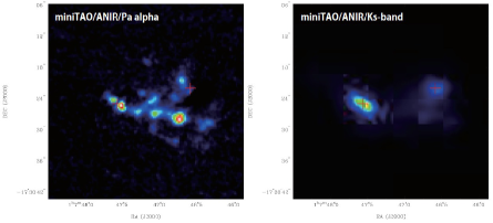
Figure 14.— The Pa$\alpha$ and $K_{\rm{s}}$ band images of VV 114 with miniTAO/ANIR observation (Tateuchi et al., 2012).

A.2. Channel maps of each line emission

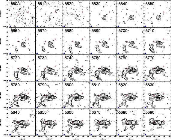
Figure 15.— The velocity channel maps of the ¹²CO (1–0) line emission of VV 114. Two crosses in each channel show the positions of the nuclei defined by the peak positions of the Ks-band observation (Tateuchi et al., 2012). The velocity width of each channel is 10 km s^-1. The beam size is plotted in the bottom-left corner of each channel. The contours represent flux intensity levels: -4.6, 4.6, 9.2, 18.4, 36.8, 73.6, 110.4 and 147.2 mJy beam^-1.

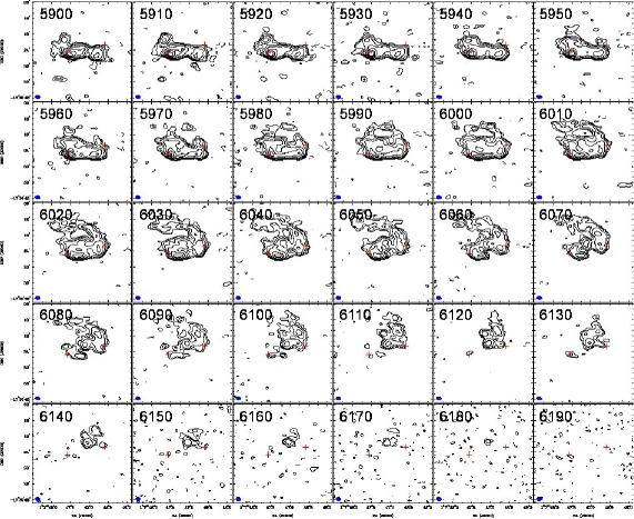
Figure 15.— Continuied.

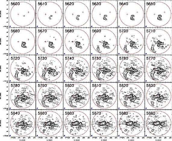
Figure 16.— The same as Figure 14 but for the CO (3–2) line emission of VV 114. The approximate field of view of ALMA 7-point mosaic at this frequency is indicated by the large red circle. The contours represent flux intensity levels: -12.6, 12.6, 25.2, 50.4, 100.8, 201.6, and 403.2 mJy beam^-1.

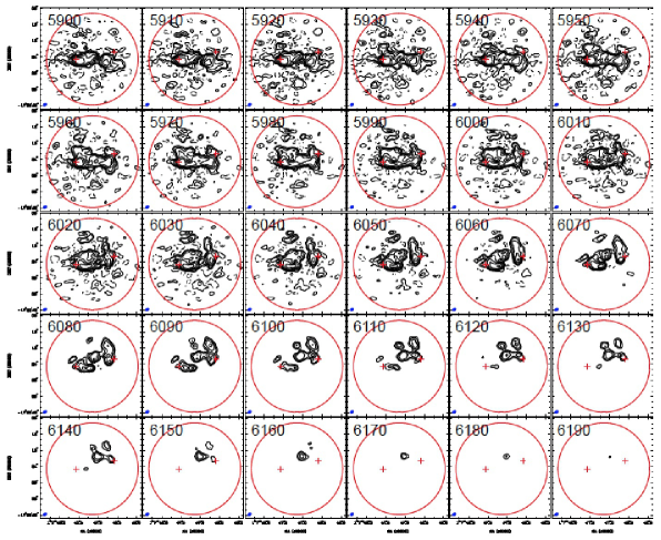
Figure 16.— Continuied.

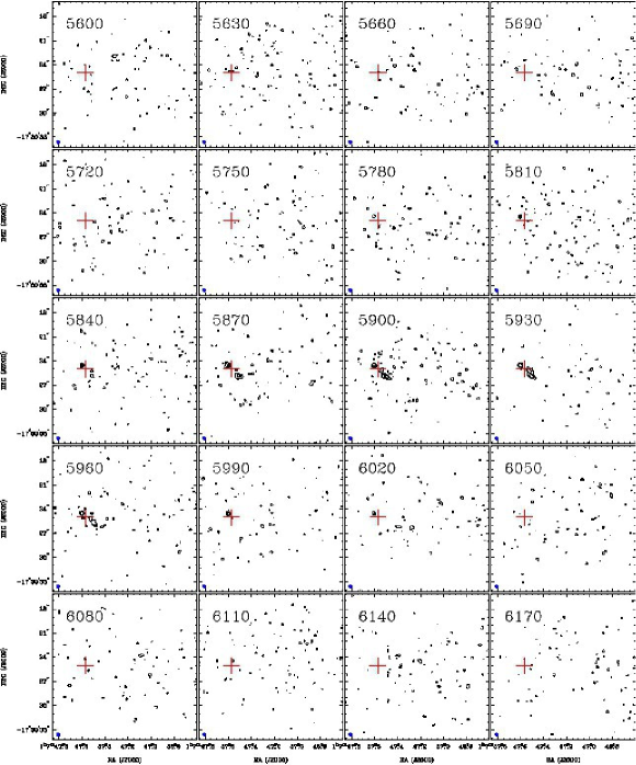
Figure 17.— The same as Figure 14 but for the HCN (4–3) line emission of VV 114. The velocity width of each channel is 30 km s^-1. The cross in each channel shows the position of the eastern nucleus defined by the peak position of the Ks-band observation (Tateuchi et al., 2012). The contours represent flux intensity levels: -2.4, 2.4, 4.8, 9.6, and 19.2 mJy beam^-1.

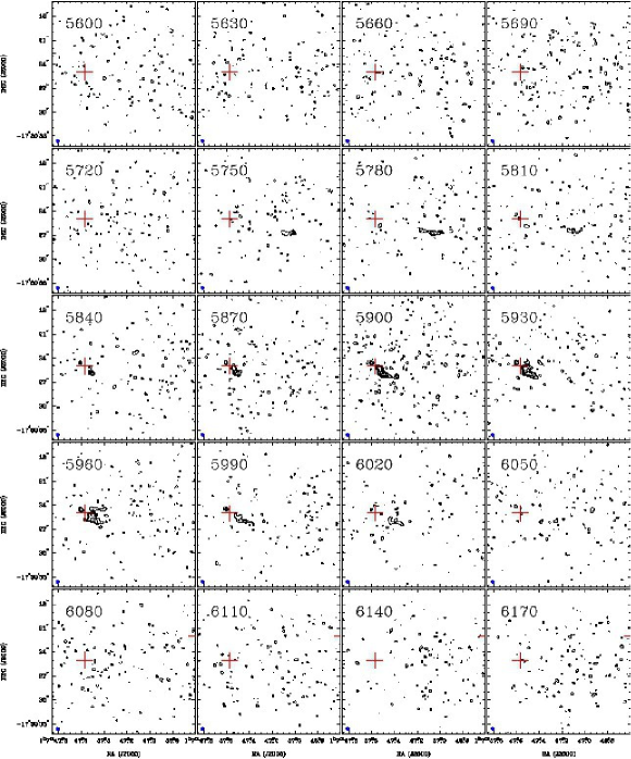
Figure 18.— The same as Figure 14 but for the HCO⁺ (4–3) line emission of VV 114. The velocity width of each channel is 30 km s^-1. The cross in each channel shows the position of the eastern nucleus defined by the peak position of the Ks-band observation (Tateuchi et al., 2012). The contours represent flux intensity levels: -2.4, 2.4, 4.8, 9.6, and 19.2 mJy beam^-1.

A.3. Box-summed spectra of each line emission

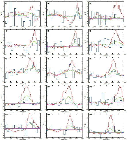
Figure 19.— 2$\farcs$0 box-summed spectra of ¹²CO (1–0) (red line), ¹³CO (1–0) $\times$ 10 (green broken line), and ¹²CO (3–2) (blue broken line) at the each box, labeled R1 - R39 of Fig 7. The spectra are taken from the ALMA data cubes after correcting the cubes for the primary beam attenuation and convolving them to 2$\farcs$0 $\times$ 1$\farcs$5 resolution (P.A. = 83 deg).

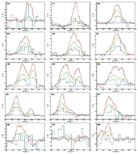
Figure 19.— continued.

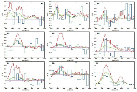
Figure 19.— continued.

Figure 20.— 2$\farcs$0 box-summed spectra of ¹²CO (3–2) (red line), CN (1_3/2–0_1/2) $\times$ 10 (green broken line), CS (2–1) $\times$ 10 (blue broken line), and CH₃OH (2_k–1_k) $\times$ 10 (light blue broken line) at R18, R21, and R39, of Fig 7. The spectra are taken from the ALMA data cubes after correcting the cubes for the primary beam attenuation and convolving them to 2$\farcs$0 $\times$ 1$\farcs$5 resolution (P.A. = 83 deg).

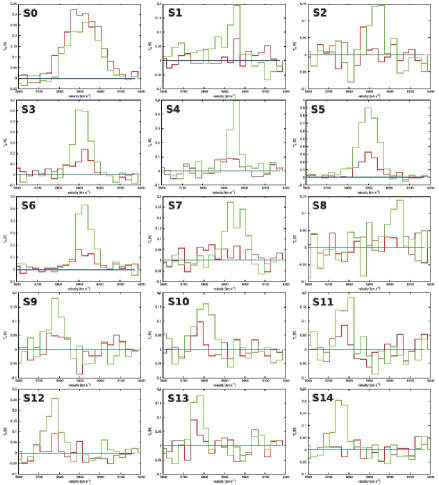
Figure 21.— 0$\farcs$5 box-summed spectra of HCN (4–3) (red line) and HCO⁺ (4–3) (green broken line) at the each box, labeled S0 - S14, of Fig 7.

References

- Aalto et al. (1995) Aalto, S., Booth, R. S., Black, J. H., & Johansson, L. E. B. 1995, A&A, 300, 369
- Aalto et al. (1997) Aalto, S., Radford, S. J. E., Scoville, N. Z., & Sargent, A. I. 1997, ApJ, 475, L107
- Aalto et al. (2010) Aalto, S., Beswick, R., Jutte, E. 2010, A&A, 522, A59
- Aladro et al. (2011) Aladro, R., Martín, S., Martín-Pintado, J., et al. 2011, A&A, 535, A84
- Alonso-Herrero et al. (2002) Alonso-Herrero, A., Rieke, G. H., Rieke, M. J., & Scoville, N. Z. 2002, AJ, 124, 166
- Armus et al. (2009) Armus, L., Mazzarella, J. M., Evans, A. S., et al. 2009, PASP, 121, 559
- Blake et al. (1987) Blake, G. A., Sutton, E. C., Masson, C. R., & Phillips, T. G. 1987, ApJ, 315, 621
- Bolatto et al. (2013) Bolatto, A. D., Wolfire, M., & Leroy, A. K. 2013, ARA&A, 51, 207
- Bournaud et al. (2011) Bournaud, F., Powell, L. C., Chapon, D., & Teyssier, R. 2011, IAU Symposium, 271, 160
- Braine et al. (2000) Braine, J., Lisenfeld, U., Due, P.-A., & Leon, S. 2000, Nature, 403, 867
- Braine et al. (2001) Braine, J., Duc, P.-A., Lisenfeld, U., et al. 2001, A&A, 378, 51
- Briggs & Cornwell (1992) Briggs, D. S., & Cornwell, T. J. 1992, Astronomical Data Analysis Software and Systems I, 25, 170
- Casoli et al. (1992) Casoli, F., Dupraz, C., & Combes, F. 1992, A&A, 264, 55
- Condon et al. (1991) Condon, J. J., Huang, Z.-P., Yin, Q. F., & Thuan, T. X. 1991, ApJ, 378, 65
- Contini & Contini (2003) Contini, M., & Contini, T. 2003, MNRAS, 342, 299
- Daddi et al. (2010) Daddi, E., Elbaz, D., Walter, F., et al. 2010, ApJ, 714, L118
- Davis et al. (2013) Davis, T. A., Heiderman, A., Evans, N. J., & Iono, D. 2013, MNRAS, 436, 570
- Downes & Solomon (1998) Downes, D., & Solomon, P. M. 1998, ApJ, 507, 615
- Draine & Lee (1984) Draine, B. T., & Lee, H. M. 1984, ApJ, 285, 89
- Engel et al. (2010) Engel, H., Davies, R. I., Genzel, R., et al. 2010, A&A, 524, A56
- Evans (2008) Evans, A. S. 2008, Frontiers of Astrophysics: A Celebration of NRAO’s 50th Anniversary, 395, 113
- Fernández-Ontiveros et al. (2009) Fernández-Ontiveros, J. A., Prieto, M. A., & Acosta-Pulido, J. A. 2009, MNRAS, 392, L16
- Frayer et al. (1999) Frayer, D. T., Ivison, R. J., Smail, I., Yun, M. S., & Armus, L. 1999, AJ, 118, 139
- Fujii et al. (2014) Fujii, K., Minamidani, T., Mizuno, N., et al. 2014, ApJ, 796, 123
- Gao et al. (2001) Gao, Y., Lo, K. Y., Lee, S.-W., & Lee, T.-H. 2001, ApJ, 548, 172
- Gao & Solomon (2004) Gao, Y., & Solomon, P. M. 2004, ApJ, 606, 271
- Garcia-Burillo et al. (2014) Garcia-Burillo, S., Combes, F., Usero, A., et al. 2014, arXiv:1405.7706
- Genzel et al. (2010) Genzel, R., Tacconi, L. J., Gracia-Carpio, J., et al. 2010, MNRAS, 407, 2091
- Grimes et al. (2006) Grimes, J. P., Heckman, T., Hoopes, C., et al. 2006, ApJ, 648, 310
- Harada et al. (2013) Harada, N., Thompson, T. A., & Herbst, E. 2013, ApJ, 765, 108
- Henkel et al. (1988) Henkel, C., Schilke, P., & Mauersberger, R. 1988, A&A, 201, L23
- Henkel et al. (2014) Henkel, C., Asiri, H., Ao, Y., et al. 2014, A&A, 565, A3
- Henning et al. (1995) Henning, T., Michel, B., & Stognienko, R. 1995, Planet. Space Sci., 43, 1333
- Hibbard et al. (2001) Hibbard, J. E., van der Hulst, J. M., Barnes, J. E., & Rich, R. M. 2001, AJ, 122, 2969
- Hildebrand (1983) Hildebrand, R. H. 1983, QJRAS, 24, 267
- Högbom (1974) Högbom, J. A. 1974, A&AS, 15, 417
- Hopkins et al. (2006) Hopkins, P. F., Hernquist, L., Cox, T. J., et al. 2006, ApJS, 163, 1
- Hopkins et al. (2013) Hopkins, P. F., Cox, T. J., Hernquist, L., et al. 2013, MNRAS, 430, 1901
- Huettemeister et al. (1997) Huettemeister, S., Mauersberger, R., & Henkel, C. 1997, A&A, 326, 59
- Imanishi et al. (2007) Imanishi, M., Nakanishi, K., Tamura, Y., Oi, N., & Kohno, K. 2007, AJ, 134, 2366
- Imanishi & Nakanishi (2013) Imanishi, M., & Nakanishi, K. 2013, AJ, 146, 91
- Imanishi & Nakanishi (2014) Imanishi, M., & Nakanishi, K. 2014, AJ, 148, 9
- Iono et al. (2004) Iono, D., Ho, P. T. P., Yun, M. S., et al. 2004, ApJ, 616, L63
- Iono et al. (2005) Iono, D., Yun, M. S., & Ho, P. T. P. 2005, ApJS, 158, 1
- Iono et al. (2007) Iono, D., Wilson, C. D., Takakuwa, S., et al. 2007, ApJ, 659, 283
- Iono et al. (2013) Iono, D., Saito, T., Yun, M. S., et al. 2013, PASJ, 65, L7
- Izumi et al. (2013) Izumi, T., Kohno, K., Martín, S., et al. 2013, PASJ, 65, 100
- Jackson et al. (1995) Jackson, J. M., Paglione, T. A. D., Carlstrom, J. E., & Rieu, N.-Q. 1995, ApJ, 438, 695
- Kartaltepe et al. (2010) Kartaltepe, J. S., Sanders, D. B., Le Floc’h, E., et al. 2010, ApJ, 721, 98
- Kennicutt (1998) Kennicutt, R. C., Jr. 1998, ApJ, 498, 541
- Kohno et al. (2001) Kohno, K., Matsushita, S., Vila-Vilaró, B., et al. 2001, The Central Kiloparsec of Starbursts and AGN: The La Palma Connection, 249, 672
- Komugi et al. (2005) Komugi, S., Sofue, Y., Nakanishi, H., Onodera, S., & Egusa, F. 2005, PASJ, 57, 733
- Konstantopoulos et al. (2009) Konstantopoulos, I. S., Bastian, N., Smith, L. J., et al. 2009, ApJ, 701, 1015
- Krips et al. (2008) Krips, M., Neri, R., García-Burillo, S., et al. 2008, ApJ, 677, 262
- Langer & Graedel (1989) Langer, W. D., & Graedel, T. E. 1989, ApJS, 69, 241
- Le Floc’h et al. (2002) Le Floc’h, E., Charmandaris, V., Laurent, O., et al. 2002, A&A, 391, 417
- Leroy et al. (2013) Leroy, A. K., Walter, F., Sandstrom, K., et al. 2013, AJ, 146, 19
- Maloney et al. (1996) Maloney, P. R., Hollenbach, D. J., & Tielens, A. G. G. M. 1996, ApJ, 466, 561
- Mao et al. (2000) Mao, R. Q., Henkel, C., Schulz, A., et al. 2000, A&A, 358, 433
- Martín et al. (2006) Martín, S., Mauersberger, R., Martín-Pintado, J., Henkel, C., & García-Burillo, S. 2006, ApJS, 164, 450
- Mauersberger et al. (1989) Mauersberger, R., Henkel, C., Wilson, T. L., & Harju, J. 1989, A&A, 226, L5
- McMullin et al. (2007) McMullin, J. P., Waters, B., Schiebel, D., Young, W., & Golap, K. 2007, Astronomical Data Analysis Software and Systems XVI, 376, 127
- Minamidani et al. (2008) Minamidani, T., Mizuno, N., Mizuno, Y., et al. 2008, ApJS, 175, 485
- Scoville et al. (2014) Scoville, N., Aussel, H., Sheth, K., et al. 2014, ApJ, 783, 84
- Papadopoulos et al. (2012) Papadopoulos, P. P., van der Werf, P. P., Xilouris, E. M., et al. 2012, MNRAS, 426, 2601
- Rich et al. (2011) Rich, J. A., Kewley, L. J., & Dopita, M. A. 2011, ApJ, 734, 87
- Saito et al. (2013) Saito, T., Iono, D., Yun, M., et al. 2013, Astronomical Society of the Pacific Conference Series, 476, 287
- Sakamoto et al. (2014) Sakamoto, K., Aalto, S., Combes, F., Evans, A., & Peck, A. 2014, arXiv:1403.7117
- Sanders et al. (1991) Sanders, D. B., Scoville, N. Z., & Soifer, B. T. 1991, ApJ, 370, 158
- Schmidt (1959) Schmidt, M. 1959, ApJ, 129, 243
- Schöier et al. (2005) Schöier, F. L., van der Tak, F. F. S., van Dishoeck, E. F., & Black, J. H. 2005, A&A, 432, 369
- Seaquist & Frayer (2000) Seaquist, E. R., & Frayer, D. T. 2000, ApJ, 540, 765
- Seaquist et al. (2004) Seaquist, E., Yao, L., Dunne, L., & Cameron, H. 2004, MNRAS, 349, 1428
- Sheffer et al. (1992) Sheffer, Y., Federman, S. R., Lambert, D. L., & Cardelli, J. A. 1992, ApJ, 397, 482
- Sliwa et al. (2013) Sliwa, K., Wilson, C. D., Krips, M., et al. 2013, ApJ, 777, 126
- Soifer et al. (1987) Soifer, B. T., Sanders, D. B., Madore, B. F., et al. 1987, ApJ, 320, 238
- Solomon & Vanden Bout (2005) Solomon, P. M., & Vanden Bout, P. A. 2005, ARA&A, 43, 677
- Sternberg & Dalgarno (1995) Sternberg, A., & Dalgarno, A. 1995, ApJS, 99, 565
- Tamura et al. (2014) Tamura, Y., Saito, T., Tsuru, T. G., et al. 2014, ApJ, 781, L39
- Tateuchi et al. (2012) Tateuchi, K., Motohara, K., Konishi, M., et al. 2012, Publication of Korean Astronomical Society, 27, 297
- Teyssier et al. (2010) Teyssier, R., Chapon, D., & Bournaud, F. 2010, ApJ, 720, L149
- Thompson et al. (2001) Thompson, A. R., Moran, J. M., & Swenson, G. W., Jr. 2001, ”Interferometry and synthesis in radio astronomy by A. Richard Thompson, James M. Moran, and George W. Swenson, Jr. 2nd ed. New York : Wiley, c2001.xxiii, 692 p. : ill. ; 25 cm. ”A Wiley-Interscience publication.” Includes bibliographical references and indexes. ISBN : 0471254924”
- Tsai et al. (2012) Tsai, M., Hwang, C.-Y., Matsushita, S., Baker, A. J., & Espada, D. 2012, ApJ, 746, 129
- Ueda et al. (2012) Ueda, J., Iono, D., Petitpas, G., et al. 2012, ApJ, 745, 65
- Ueda et al. (2014) Ueda, J., Iono, D., Yun, M. S., et al. 2014, ApJS, 214, 1
- van Dishoeck & Black (1988) van Dishoeck, E. F., & Black, J. H. 1988, ApJ, 334, 771
- van der Tak et al. (2007) van der Tak, F. F. S., Black, J. H., Schöier, F. L., Jansen, D. J., & van Dishoeck, E. F. 2007, A&A, 468, 627
- Warren et al. (2010) Warren, B. E., Wilson, C. D., Israel, F. P., et al. 2010, ApJ, 714, 571
- Wild et al. (1992) Wild, W., Harris, A. I., Eckart, A., et al. 1992, A&A, 265, 447
- Wilson et al. (2003) Wilson, C. D., Scoville, N., Madden, S. C., & Charmandaris, V. 2003, ApJ, 599, 1049
- Wilson et al. (2008) Wilson, C. D., Petitpas, G. R., Iono, D., et al. 2008, ApJS, 178, 189
- Wilson et al. (2014) Wilson, C. D., Rangwala, N., Glenn, J., et al. 2014, ApJ, 789, L36
- Wilson et al. (2009) Wilson, T. L., Rohlfs, K., Huttemeister, S. 2009, Tools of Radio Astronomy, by Thomas L. Wilson; Kristen Rohlfs and Susanne Hüttemeister. ISBN 978-3-540-85121-9. Published by Springer-Verlag, Berlin, Germany, 2009.,
- Wilson & Rood (1994) Wilson, T. L., & Rood, R. 1994, ARA&A, 32, 191
- Yao et al. (2003) Yao, L., Seaquist, E. R., Kuno, N., & Dunne, L. 2003, ApJ, 588, 771
- Yun et al. (1994) Yun, M. S., Scoville, N. Z., & Knop, R. A. 1994, ApJ, 430, L109
- Zhu et al. (2003) Zhu, M., Seaquist, E. R., & Kuno, N. 2003, ApJ, 588, 243
- Zhu et al. (2007) Zhu, M., Gao, Y., Seaquist, E. R., & Dunne, L. 2007, AJ, 134, 118