Pointwise estimates and regularity in geometric optics and other Generated Jacobian equations

Abstract.

The study of reflector surfaces in geometric optics necessitates the analysis of certain nonlinear equations of Monge-Ampère type known as generated Jacobian equations. This class of equations, whose general existence theory has been recently developed by Trudinger, goes beyond the framework of optimal transport. We obtain pointwise estimates for weak solutions of such equations under minimal structural and regularity assumptions, covering situations analogous to that of costs satisfying the A3-weak condition introduced by Ma, Trudinger and Wang in optimal transport. These estimates are used to develop a $C^{1,\alpha}$ regularity theory for weak solutions of Aleksandrov type. The results are new even for all known near-field reflector/refractor models, including the point source and parallel beam reflectors and are applicable to problems in other areas of geometry, such as the generalized Minkowski problem.

1. Introduction

1.1. Overview.

This paper is concerned with the regularity theory of a broad class of Monge-Ampère type equations spanning optimal transport and geometric optics. These may sometimes lie outside the scope of optimal transport but always have a Jacobian structure, namely

$$\textnormal{det}(D[T(x,Du,u)])=\psi(x,Du,u),$$ (1.1)

for some $T:dom(T)\subseteq\Omega\times\mathbb{R}^{d}\times\mathbb{R}\to\mathbb{R}^{d}$ (see below). Admissible $u$ are “convex”, i.e.

$$D[T(x,Du,u)]\geq 0,$$

which is necessary for (1.1) to be a degenerate elliptic PDE. To appreciate the generality of (1.1), note it covers the real Monge-Ampére equation, the $c$-Monge-Ampére equation from optimal transport with cost $c$, the point source near-field reflector problem from geometric optics, several variations of the Minkowski problem and principal-agent problems in economics when dealing with a non-quasilinear utility function (references to the relevant literature are given below, see also Section 3). Some of the corresponding $T$’s are

$$T(x,\bar{p},u) =\bar{p} \textnormal{(real Monge-Amp\'{e}re equation)},$$

$$(D_{x}c)(x,T(x,\bar{p},u)) =-\bar{p} \textnormal{(Optimal transport with cost $c(\cdot,\cdot)$)},$$

$$T(x,\bar{p},u) =\frac{\bar{p}}{|\bar{p}|^{2}-(u-\bar{p}\cdot x)^{2}} \textnormal{(Point source near-field reflector)}.$$

These and other examples will be discussed further in Section 3. The mappings $T(x,\bar{p},u)$ considered here will always be given by a generating function. This means there is a function $G:dom(G)\subseteq M\times\bar{M}\times\mathbb{R}\to\mathbb{R}$ and associated “exponential mappings” $\textnormal{exp}^{G}_{x,u}(\cdot),Z^{G}_{x}(\cdot,\cdot)$ (see Section 4 for definitions) such that

$$T(x,\bar{p},u)=\textnormal{exp}^{G}_{x,u}(\bar{p}).$$

For such $T$’s, (1.1) takes the form

$$\textnormal{det}(D^{2}u+(D^{2}_{x}G)(x,\textnormal{exp}^{G}_{x,u}(Du),Z^{G}_{x}(Du,u)))=\psi_{G}(x,Du,u).$$ (GJE)

The corresponding convexity condition for $u$ asks that it be of the form

$$u(x)=\sup\limits_{\bar{x}}\limits G(x,\bar{x},z_{\bar{x}})$$

for some function $\bar{x}\to z_{\bar{x}}\in\mathbb{R}$, $\bar{x}\in\bar{M}$. Following work of Trudinger [Tru14b], where the general framework for these equations is proposed, equation (GJE) will be called a “Generated Jacobian Equation.” The distinguishing feature of (GJE) is the dependence of the mapping $T$ on the values of the solution, which is not present in the case of optimal transport. Recall that in optimal transport, one has

$$G(x,\bar{x},z) =-c(x,\bar{x})+z,$$

$$T(x,\bar{p},u) =T(x,\bar{p})=exp^{c}_{x}({\bar{p}})$$

where $c(x,\bar{x})$ denotes the cost function. In general, changing the “height” parameter $z$ in $G(x,\bar{x},z)$ will result in a change in the shape of the function, and not merely a vertical shift; and the choice of coordinate systems must now take this into account.

The aim of this work is to determine the differentiability of weak solutions to (GJE) under minimal on assumptions on the data (including the generating function $G$, and the function $\psi_{G}$). Specifically, we focus on weak solutions to (GJE) in the “Aleksandrov sense”, we also require the right hand side of the equation to bounded away from zero and infinity. The notion of Aleksandrov solution originated in the study of the real Monge-Ampère equation and has also played a key role in optimal transport, see Definition 4.16 for the setting of generated Jacobian equations. Our results are new even for the case of near-field reflector/refractor problems, covering situations where the condition (G3s) fails but (G3w) still holds. The (G3w) condition was introduced by Trudinger in [Tru14b], it generalizes (A3w) condition for the Ma-Trudinger-Wang tensor [MTW05]. Both the MTW tensor and the (A3w) condition play a central role in the regularity theory of optimal transport.

This general framework makes our results applicable to problems beyond geometric optics. Roughly speaking, these results are in the same vein as Caffarelli’s localization and differentiability estimate for the real Monge-Ampére equation [Caf90b]; Figalli, Kim, and McCann’s regularity theory for optimal transport maps under the (A3w) condition [FKM13a], as well as work by Vétois [Vét15], and by the authors on the strict $c$-convexity of $c$-convex potentials [GK15].

In the spirit of [GK15], the most important assumption on $G$ is a synthetic version of (G3w), which is roughly a “quantitative quasiconvexity” condition along $G$-segments ($G$-QQConv). This condition follows from (G3w) when $G$ is smooth enough, it generalizes the (QQConv) condition introduced in [GK15] for optimal transport (and in that case, it refines Loeper’s maximum principle).

Our main results can be broadly separated in two parts. The first part consists of pointwise inequalities, Theorems 2.1 and 2.2, for $G$-convex functions $u$ (see Definition 4.14). These are obtained under natural assumptions on $G$ and $u$, one of the key conditions being ($G$-QQConv) mentioned above. The pointwise inequalities may be thought of as nonlinear analogues of the Blaschke-Santaló inequalities for the Mahler volume (see discussion in Section 1.2)

The second part comprises Theorems 2.3 and 2.4, in which we prove strict $G$-convexity and interior $C^{1,\alpha}$ differentiability respectively of weak solutions $u$ of (1.1). This part relies on the pointwise inequalities in Theorems 2.1 and 2.2 to show solutions satisfy a localization property (which leads to strict convexity) and an engulfing property (which leads to interior $C^{1,\alpha}$ estimates). Finally, we show that for $G$ smooth enough, condition ($G$-QQConv) is implied by (G3w) (Theorem 2.5). Precise statements for these results are given in Section 2.

Acknowledgements. The authors would like to thank Neil Trudinger for helpful correspondence and also for graciously sharing some of his unpublished work. The authors would also like to express their gratitude to the anonymous referee for their prompt and thorough reading of the manuscript, as well as suggested improvements.

1.2. Strategy: Mahler volume and Monge-Ampére equations.

In order to motivate the main results (Section 2) it will be convenient to recall several facts about the Mahler volume and relate it to the regularity theory for the real Monge-Ampére equation. Let $S$ be a convex set with non-empty interior and whose center of mass is $0$. The Mahler volume of $S$, $m(S)$, is defined as

$$m(S):=\left|{S}\right|_{\mathcal{L}}\left|{S^{*}}\right|_{\mathcal{L}},$$

where the set $S^{*}$ is the polar dual of $S$,

$$S^{*}:=\{y\in\mathbb{R}^{n}\mid(x^{\prime},y)\leq 1,\;\;\forall\;x^{\prime}\in S\}.$$

Then, the celebrated Blashke-Santaló and reverse Santaló inequalities together say that

$$c_{n}^{-1}\;\leq\left|{S}\right|_{\mathcal{L}}\left|{S^{*}}\right|_{\mathcal{L}}\leq c_{n}.$$ (1.2)

These geometric inequalities imply (and are in fact equivalent) to certain pointwise inequalities for convex functions. Suppose a convex function $u:\mathbb{R}^{n}\to\mathbb{R}$ and an affine function $l$ are such that the set $S:=\{u<l\}$ is nonempty, bounded, and with center of mass at $0$. Then, one can use (1.2) to prove the bounds

$$\sup\limits_{S}(l-u)^{n}\geq C_{n}^{-1}\left|{S}\right|_{\mathcal{L}}\left|{\partial{u}{(\tfrac{1}{2}S)}}\right|_{\mathcal{L}},$$ (1.3)

$$(l(x)-u(x))^{n}\leq C_{n}\left|{S}\right|_{\mathcal{L}}\left|{\partial{u}{(S)}}\right|_{\mathcal{L}},\;\;\forall\;x\in S.$$ (1.4)

These two estimates are crucial in the theory of the Monge-Ampère equation, in fact, they are the basis of Caffarelli’s theorem on the strict convexity and differentiability of Aleksandrov solutions of the real Monge-Ampére equation [Caf90b] (see the discussion in [Caf92a, Part 2], and the discussion in [GK15, Section 1.3]). For now let us explain informally how these estimates may be used to obtain regularity to solutions of the Monge-Ampère equation, namely $C^{1,1}$ regularity and strong convexity. Note first that a convex function $u$ is $C^{1,1}$ and strongly convex if and only if there is a $C>0$ such that for any supporting affine function $l_{0}$ and every small enough $h>0$ we have the inclusions

$$B_{C^{-1}\sqrt{h}}\subset\{u\leq l_{0}+h\}\subset B_{C\sqrt{h}}.$$ (1.5)

In other words, the level sets of $u$ are comparable to those of a paraboloid. Now, let $u$ be an Aleksandrov solution to $\textnormal{det}(D^{2}u)=f$, with $\lambda\leq f\leq\Lambda$ (see Definition 4.16). Let us see to what extent would something like (1.5) hold for $u$. Since $u$ is an Aleksandrov solution, we have $\left|{\partial{u}{(S)}}\right|_{\mathcal{L}}\sim\left|{S}\right|_{\mathcal{L}}$, in which case estimates (1.3)-(1.4) imply

$$\left|{B_{C^{-1}\sqrt{h}}}\right|_{\mathcal{L}}\leq\left|{\{u\leq l_{0}+h\}}\right|_{\mathcal{L}}\leq\left|{B_{C\sqrt{h}}}\right|_{\mathcal{L}}$$ (1.6)

for some $C>0$. This is a weaker assertion than (1.5), since we only compare the measures of the sublevel sets. The approach introduced by Caffarelli in the context of the real Monge-Ampére equation [Caf90b, Caf91, Caf92b] shows how to go beyond (1.6) and obtain $C^{1,\alpha}$ regularity and strict convexity for $u$, and even (1.5) and higher regularity if $f$ is assumed to be regular. See Gutiérrez’s book [Gut01] for a comprehensive exposition of these ideas.

For the $c$-Monge-Ampére equation arising in optimal transport, Figalli, Kim, and McCann obtained [FKM13a] analogues of (1.3)-(1.4) under the (A3w) assumption of Ma, Trudinger and Wang, from where they obtained $C^{1,\alpha}$ and strict $c$-convexity estimates. In [GK15] the authors introduced a condition on costs, “quantitative quasiconvexity” (QQConv), and used it to derive analogues of (1.3)-(1.4). This (QQConv) condition is a refinement of Loeper’s “maximum principle” [Loe09] but at least for $C^{4}$ costs turns out to be equivalent to (A3w) (and thus to Loeper’s condition itself).

Beyond $C^{1,\alpha}$ and $C^{2,\alpha}$ estimates, these inequalities are also an important tool in deriving $W^{2,p}$ estimates [Caf90a] under extra assumptions on $f$, and more recently $W^{2,1+\epsilon}$ estimates under minimal assumptions [DPF13, DPFS13]. See the survey by Figalli and De Philippis [DPF14] for a thorough discussion of recent optimal transport literature (see also Section 3).

1.3. Notation.

Before continuing with the introduction, let us set up some notational conventions used within the paper: $\langle\cdot,\cdot\rangle$ will denote the evaluation pairing between an element of a vector space and an element of its dual space. $(M,g),(\bar{M},\bar{g})$ will denote $n$-dimensional complete Riemannian manifolds. Points in $M$ will be denoted with $x,y...$ points in $\bar{M}$ will be denoted with $\bar{x},\bar{y},...$ while $\left|{\cdot}\right|_{\mathcal{L}}$ will denote the Riemannian volume on $(M,g)$, $(\bar{M},\bar{g})$, or the associated Riemannian volumes on a tangent or cotangent space. $\lvert\cdot\rvert_{g_{x}}$ and $\lvert\cdot\rvert_{\bar{g}_{\bar{x}}}$ will denote the length of tangent or cotangent vectors, with respect to the inner products $g_{x}$ and $\bar{g}_{\bar{x}}$, and $d_{g}{\left(\cdot,\cdot\right)}$, $d_{\bar{g}}{\left(\cdot,\cdot\right)}$ will refer to the geodesic distances induced by the respective metrics. Also, we will use $A^{\operatorname{int}}$, $A^{\operatorname{cl}}$, and $A^{\partial}$ to refer to the interior, closure, and boundary of a set $A$ respectively.

Here is a summary of several other symbols, together with their definition number.

Notation / Condition	Name	Definition location
$G$, $H$	Generating function, dual function	Section 4.1
$\mathfrak{g},\mathfrak{h}$		Section 4.1
(Unif), ($\textnormal{Lip}_{K_{0}}$), $K_{0}$		Definition 4.1
($G$-Twist), (${G^{\ast}}$-Twist)		Definition 4.3
($G$-Nondeg)		Definition 4.5
$E(x,\bar{x},z)$, $\bar{E}(x,\bar{x},z)$		Definition 4.5
$p_{\bar{x},z}(x)$, $\bar{p}_{x,u}(\bar{x})$		Definition 4.6
$[\bar{A}]_{x,u}$, $[A]_{\bar{x},z}$		Definition 4.6
$\left[x_{0},x_{1}\right]_{\bar{x},z}$	$G$-segment	Remark 4.9
$\textnormal{exp}^{G}_{\bar{x},z}(\cdot)$, $\textnormal{exp}^{G}_{x,u}(\cdot)$, $Z^{G}_{x}(\cdot,\cdot)$	$G$-exponential mappings	Definition 4.7
(DomConv∗), (DomConv)		Definition 4.11
($G$-QQConv), (${G^{\ast}}$-QQConv)		Definition 4.13
$m,m_{0},\ldots$	$G$-affine functions	Definition 4.14
$u,u_{0},\ldots$	$G$-convex functions	Definition 4.14
$\partial_{G}u$	$G$-subdifferential	Definition 4.15
	nice, very nice functions	Definition 4.18
	very nice constant	Remark 4.29
$A^{*}_{p,q,\lambda}$	Polar dual	Definition 6.2
$A^{G}_{x,m,\lambda}$	$G$-dual	Definition 4.22
$K^{G}_{x,S}(\cdot)$	$G$-cone	Definition 4.25
$\Pi^{\omega}_{A}$	Supporting hyperplane	Definition 5.1

2. Statement of main results

In this section we state the exact form of our main results. The precise statement themselves involve a great deal of notation that will not be introduced until Section 4, however, for the sake of having all the main results stated in one section, we choose to present them here. Thus, the reader is advised to skim through this section on a first reading and return to it after reading the elements of generating functions in Section 4.

Structural assumptions. All of the theorems below require a number of structural assumptions on $G$ and its domain of definition. In many important subclasses of examples (i.e. optimal transport, near field problems in optics) each of these structural assumptions are known to be necessary conditions for the regularity of solutions.

Then, we are given $n$-dimensional Riemannian manifolds $M,\bar{M}$, a generating function which is a function $G:M\times\bar{M}\times{\mathbb{R}}\to\mathbb{R}$; we are also given domains $\Omega\subset M$, $\bar{\Omega}\subset\bar{M}$, and $\mathfrak{g}\subset M\times\bar{M}\times{\mathbb{R}}$. We assume these objects have the following properties (see Section 4 for details)

$$\begin{array}[]{l}\textnormal{(I)}\;G(x,\bar{x},z)\textnormal{ is }C^{2}\textnormal{ in the sense that all purely mixed second derivatives exist and are }\\ \text{continuous in all of }M\times\bar{M}\times{\mathbb{R}}.\;\textnormal{ Moreover, }G_{z}<0.\\ \\ \textnormal{(II)}\;\;\textnormal{There are constants }-\infty\leq\underline{u}<\overline{u}\leq\infty\textnormal{ and }K_{0}>0\textnormal{ such that }\Omega,\bar{\Omega},\textnormal{ and }\mathfrak{g}\textnormal{ satisfy}\\ \textnormal{\eqref{G5}, \eqref{Lip}, \eqref{DomConv}, and \eqref{DualDomConv}}\textnormal{ with respect to the interval }(\underline{u},\overline{u}).\\ \\ \textnormal{(III)}\;G\textnormal{ satisfies }\eqref{Twist},\eqref{DualTwist},\eqref{Nondeg},\eqref{QQConv}\textnormal{ and }\eqref{DualQQConv}.\\ \end{array}$$

We are also given a function $u$ (eventually, the solution to (GJE)), assumed to satisfy the following (see Definition 4.18 and Remarks 4.20 and 4.29)

$$\textnormal{(IV) }u:\Omega\to\mathbb{R}\textnormal{ is a \emph{very nice} }G\textnormal{-convex function with an associated}\;\;\;\;\quad\quad\quad\quad\quad\quad\quad$$

$$\textnormal{\emph{very nice} interval }[\underline{u}_{\rm N},\overline{u}_{\rm N}].\quad\quad\quad\quad\quad\quad\quad\quad\quad\quad\quad\quad\quad\quad\quad\quad\quad\quad\quad\quad\quad\quad\quad\quad\quad\quad$$

Remark.

The notion of very nice for a $G$-convex function is explained in Definition 4.18, this notion is irrelevant in optimal transport, where all $G$-convex functions are automatically very nice. The necessity for this notion for general Generated Jacobian equations is illustrated by phenomena present in the near field problem (see Karakhanyan and Wang [KW10, Theorem A,B]). This is discussed in detail at the end of Section 3.1.

Finally, in all what follows $M\geq 1$ will denote the constant associated to $G$ by ($G$-QQConv) and (${G^{\ast}}$-QQConv) with the interval $[\underline{u}_{\rm N},\overline{u}_{\rm N}]$.

The first result is an Aleksandrov type estimate, which will play the role that (1.4) plays for the standard Monge-Ampére theory.

Theorem 2.1.

Suppose $m(\cdot):=G(\cdot,\bar{x},z)$ for some $(\bar{x},z)\in\bar{\Omega}\times{\mathbb{R}}$ is a nice $G$-affine function and $S:=\left\{u\leq m\right\}$. Also assume that $[S]_{\bar{x},z}\subset B\subset 3B\subset[\Omega]_{\bar{x},z}$ for some ball $B$ in $T^{*}_{\bar{x}}{\bar{M}}$ (which may be of any radius). Then, there exist very nice constants $\epsilon$, $C>0$ such that for any $\omega_{1}\in\mathbb{S}^{n-1}\subset T^{*}_{\bar{x}}{\bar{M}}$ and $x_{0}\in S^{\operatorname{int}}$, if $\textnormal{diam}{(S)}<\epsilon$ then

$$(m(x_{0})-u(x_{0}))^{n}\leq\frac{Cd{\left(p_{0},\Pi^{\omega_{1}}_{[S]_{\bar{x},z}}\right)}}{l([S]_{\bar{x},z},\omega_{1})}\left|{S}\right|_{\mathcal{L}}\left|{\partial_{G}u(S)}\right|_{\mathcal{L}},$$

where $p_{0}:=p_{\bar{x},z}(x_{0})$ and $l([S]_{\bar{x},z},\omega_{1})$ is defined as the maximum length among all line segments parallel to $\omega_{1}$ and contained in $[S]_{\bar{x},z}$.

The second result gives a generalization of estimate (1.3).

Theorem 2.2.

Suppose $m(\cdot):=G(\cdot,\bar{x},z)$ for some $(\bar{x},z)\in\bar{\Omega}\times{\mathbb{R}}$ is a $G$-affine function such that $\underline{u}_{\rm N}\leq m\leq\overline{u}_{\rm N}$ on $\Omega^{\operatorname{cl}}$. Writing $S:=\left\{x\in\Omega\mid u(x)\leq m(x)\right\}$, there exist very nice constants $C$, $K>0$ such that for any $A\subset\Omega$ with $[A]_{\bar{x},z}$ connected, satisfying

$$KM[A]_{\bar{x},z} \subset[S]_{\bar{x},z},$$ (2.1)

$$\sup_{A}{m}+\sup_{A}{(m-u)} <\overline{u},$$ (2.2)

we have

$$\sup_{A}{(m-u)}^{n}\geq C\left|{A}\right|_{\mathcal{L}}\left|{\partial_{G}u\left(A\right)}\right|_{\mathcal{L}}.$$

Here $KM[A]_{\bar{x},z}$ is the dilation of $[A]_{\bar{x},z}$ with respect to its center of mass $p_{\bar{x},z}(x_{cm})$.

Our next two results concern weak solutions $u$ to (GJE), in the sense of Aleksandrov (see Definition 4.16). We use the notation $\Omega_{0}$ for the support of the Radon measure $\left|{\partial_{G}u\left(\cdot\right)}\right|_{\mathcal{L}}$ and $\bar{\Omega}_{0}:=\partial_{G}u\left(\Omega_{0}\right)$. The first of the two theorems deals with the strict $G$-convexity of $u$.

Theorem 2.3.

Suppose $u$ is a very nice Aleksandrov solution of (GJE). If $\Omega_{0}^{\operatorname{cl}}\subset\Omega^{\operatorname{int}}$ and $\bar{\Omega}_{0}^{\operatorname{cl}}\subset\bar{\Omega}^{\operatorname{int}}$, and $[\bar{\Omega}_{0}]_{x_{0},u(x_{0})}$ is convex for some $x_{0}\in\Omega_{0}^{\operatorname{int}}$, then $u$ is strictly $G$-convex at $x_{0}$, i.e. if $\bar{x}_{0}\in\partial_{G}u\left(x_{0}\right)$, then the set $\left\{x\in\Omega\mid u(x)=G(x,\bar{x}_{0},H(x_{0},\bar{x}_{0},u(x_{0}))\right\}$ is the singleton $\left\{x_{0}\right\}$.

We prove (interior) $C^{1,\alpha}$ regularity of weak solutions (provided they are very nice). The proof relies on the previous theorems as well as extensions of the engulfing property of sublevelsets of solutions for the real Monge-Ampére Equation (see [FM04],[FKM13a, Section 9]).

Theorem 2.4.

Suppose in addition to the assumptions of Theorem 2.3 above, that $G$ is a $C^{1,\alpha}$ function in the $x$ variable for some $\alpha\in(0,1]$, uniformly in the $(\bar{x},z)$ variables. Then there exists an $\beta\in(0,1]$ such that $u\in C_{loc}^{1,\beta}(\Omega_{0}^{\operatorname{int}})$.

Our final result connects the (G3w) condition introduced by Trudinger [Tru14b] with the conditions ($G$-QQConv) and (${G^{\ast}}$-QQConv).

Theorem 2.5.

Assume there are $-\infty\leq\underline{u}<\overline{u}\leq\infty$ such that $\Omega$, $\bar{\Omega}$, and $\mathfrak{g}$ satisfy (Unif), (DomConv), and (DomConv^∗) with respect to $(\underline{u},\overline{u})$. Also assume $G$ is $C^{4}$, by which we mean all derivatives of up to order $4$ total, with at most two derivatives ever falling on one variable $x$, $\bar{x}$, or $z$ at once, exist and are continuous and $G$ satisfies ($G$-Twist), (${G^{\ast}}$-Twist), ($G$-Nondeg), and (G3w). Then $G$ also satisfies both ($G$-QQConv) and (${G^{\ast}}$-QQConv).

2.1. Overview of the rest of the paper.

A detailed discussion of examples of (GJE) covered by our results is carried out in Section 3, examples discussed include the near-field reflector problem and the generalized Minkowski problem. In Section 4 we review the elements of generating functions and the associated Jacobian equations (GJE) (following to a great extent the ideas in [Tru14b]), we also introduce the ($G$-QQConv) and (${G^{\ast}}$-QQConv) conditions on $G$.

In Section 5 we show how ($G$-QQConv) and (${G^{\ast}}$-QQConv) lead to the Aleksandrov-type estimate, Theorem 2.1. In Section 6 we prove the sharp growth estimate, Theorem 2.2. In Section 7 we use the pointwise estimates to prove a localization property for weak solutions, and their strict convexity (Theorem 2.3). The work of all previous sections are combined in Section 8 to prove solutions are $C^{1,\alpha}$ (Theorem 2.4).

Finally, in Section 9 we prove (Theorem 2.5) that the condition (G3w) (defined by Trudinger in [Tru14b] to obtain classical regularity in generated Jacobian equations), implies conditions ($G$-QQConv) and (${G^{\ast}}$-QQConv).

3. Examples

3.1. Point source, near-field reflector

For our first example, we spend some time discussing the near-field reflector problem, as it is a well-studied problem that gives rise to a generated Jacobian equation (GJE) which does not arise from an optimal transport problem, and as such displays many subtle difficulties not seen in the optimal transport case.

The engineering literature on reflector design is too large to review in detail here, but let us point out the reader to a few references, such as Oliker [Oli89] Kochengin and Oliver [KO98] and Janssen and Maes [JM92] for the case of cylindrical reflectors. For more on the literature and the exposition to follow, the reader is directed to the survey article [Oli03] by Oliker, the discussion in Karakhanyan and Wang [Kar14]. See also the classical monograph by Rusch and Potter [RP70] for a broader introduction to the engineering of antennas.

Figure 1.

We are given a light source at some point $O\in\mathbb{R}^{3}$, that shines through a “source region” $\Omega\subset\mathbb{S}^{2}$ and a “target region” to be illuminated, which is a region $\bar{\Omega}$ contained within some codimension one surface $\bar{M}\subset\mathbb{R}^{3}$. Moreover, the light source may not have a uniform intensity, instead it radiates energy through $\Omega$ modeled by some absolutely continuous measure $fd\textnormal{Vol}_{\mathbb{S}^{2}}$.

The goal is now to build a reflector: a (perfectly reflective) surface $\Gamma_{\rho}\subset\mathbb{R}^{3}$ given by the radial graph of some function $\rho:\Omega\to\mathbb{R}$ with the property that light emanating from $O$ according to the distribution $f$ is reflected off to arrive in $\bar{\Omega}$. This problem is severely underdetermined, thus we also assume that we are given an absolutely continuous measure $gd\textnormal{Vol}_{\bar{M}}$ supported on $\bar{\Omega}$, and the reflector is required to recreate this measure as the resulting illumination pattern. The assumption of perfect reflection implies that the total masses of $f$ and $g$ must be equal. The usual plan of attack for this problem is to first assume the geometric optics approximation, in which light rays are treated like particles, completely ignoring any wave-like behavior that may be present.

To motivate an elementary method of constructing such a desired reflector, consider the case where the target measure is not absolutely continuous, but a Dirac delta concentrated at a point $\bar{x}\in\bar{\Omega}$. Then the reflector can be taken as any ellipsoid of revolution with foci $O$ and $\bar{x}$. For $2a>\lvert\bar{x}\rvert$ there is a unique ellipsoid of revolution with foci $O$ and $\bar{x}$ whose major axis has length equal to $2a$. A straightforward computation shows that such an ellipsoid can be written as the radial graph of a function $e(\cdot,\bar{x},a):\mathbb{S}^{2}\to\mathbb{R}_{+}$ defined by

$$e(x,\bar{x},a)=\frac{a^{2}-\tfrac{1}{4}|\bar{x}|^{2}}{a-\tfrac{1}{2}\left(x,\bar{x}\right)}$$

where $\left(x,\bar{x}\right)$ is the Euclidean inner product in ${\mathbb{R}}^{3}$. We can view $a$ here as a scalar parameter controlling the eccentricity of the ellipse, in particular we see there is a one parameter family of reflectors that solve our problem.

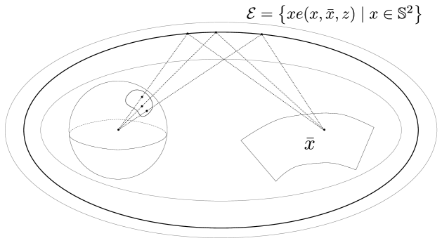
Figure 2.

If the target measure is now a finite sum of weighted Dirac deltas, we can take the reflector to be the boundary of the intersection of the same number of ellipsoids, each with one focus at $O$ and the other at a point where the sum of deltas is supported. By adjusting the scalar parameters, we can ensure each point in the target receives the correct amount of energy.

One can then approximate the absolutely continuous target measure by a sequence of such finite sums of Dirac deltas, and rigorously justify a limiting process to obtain a reflector that is the boundary of an intersection of (an infinite) family of ellipsoids, or in terms of $\rho$:

$$\rho(x)=\inf_{(\bar{x},a)\in\mathcal{A}}e(x,\bar{x},a)$$ (3.1)

for some appropriate collection $\mathcal{A}$.

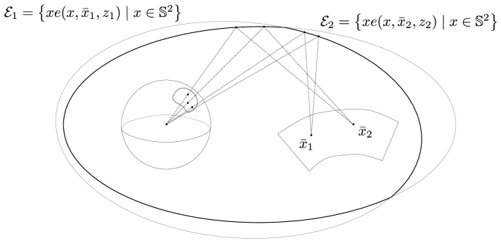
Figure 3.

This representation of $\rho$ can be interpreted as a form of “concavity” of $\rho$, where instead of hyperplanes as in the usual case of a concave function, $\rho$ is supported from above by graphs of ellipsoids which serve as some sort of “fundamental shape”. Indeed, if we take

$$G(x,\bar{x},z):=\frac{1}{e(x,\bar{x},z^{-1})},$$

defined in

$$\mathfrak{g}=\left\{(x,\bar{x},z)\in\mathbb{S}^{2}\times\bar{M}\times\mathbb{R}_{+}\mid\tfrac{1}{2}z\lvert\bar{x}\rvert<1\right\},$$

then $\rho$ will exactly be a $G$-convex function as in Definition 4.14.

When $\bar{M}$ can be written as the graph of a function over a portion of ${\mathbb{R}}^{2}$, it can easily be verified that our choice of $G$ coincides with that of Trudinger in [Tru14b, (4.15)]. In the particular case when $\bar{M}$ is contained in a hyperplane parallel to ${\mathbb{R}}^{2}$ lying below ${\mathbb{R}}^{2}$, from the formulae in [Tru14b, Section 4] it can be seen that $G$ satisfies conditions ($G$-Twist), (${G^{\ast}}$-Twist), ($G$-Nondeg), and (G3w), and (Unif) with $(\underline{u},\overline{u})=(0,\infty)$. The main difference here from the usual case of convexity / concavity (or indeed, from the optimal transport case known in the literature as $c$-convexity), is that when the scalar parameter $z$ is changed in any of the functions $e$ forming the infimum in (3.1), there is a nontrivial change in the shape that goes beyond a simple translation or dilation.

Next one can consider what is known as the ray-tracing map, a map $T_{\rho}:\Omega\to\bar{\Omega}$ that simply gives the location that a beam originating through $x$ ends up after reflecting off of $\Gamma_{\rho}$.

It can be seen that to obtain the desired illumination property, it is sufficient to impose a prescribed Jacobian equation of the form $f(x)\textnormal{det}{DT_{\rho}(x)}=g(T_{\rho}(x))$. From the form (3.1) of $\rho$, and a calculation of $T_{\rho}$ in terms of the derivative of $\rho$, this equation can be re-written as a generated Jacobian equation of the form (GJE). In fact, the choice of $u=\rho^{-1}$ will be a solution of (GJE) with our above choice of $G$, and a certain $\psi_{G}$ involving the densities $f$ and $g$.

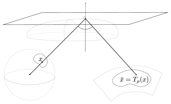
Figure 4.

It should be noted that a question of deep physical interest now is regularity of the reflector. Indeed, non differentiability of a reflector would cause diffraction phenomena, which may not be accurately modeled by the geometric optics approximation. In the case of refraction problems which also give rise to generated Jacobian equations, singularities can lead to chromatic aberrations, which also lie outside the realm of geometric optics.

Recent work of Karakhanyan and Wang [KW10] guarantees regularity ($C^{2,\alpha}$) for reflectors. Their main result illustrates some of the complexities that arise once we leave the optimal transport framework (see in particular Remark 3.1 below).

Theorem.

[KW10, see Theorems A-B] Suppose that

1. $\Omega$, $V\subset\mathbb{S}^{n-1}$, $\Omega\cap V=\emptyset$, $\Omega$ has Lipschitz boundary.

2. $\bar{\Omega}$ is a region in a convex hypersurface $\bar{M}$, given by a radial graph of some smooth function over $V$.

3. $f:\Omega\to\mathbb{R},$ $g:\bar{\Omega}\to\mathbb{R}$ smooth, strictly positive functions with the same total mass.

4. $\partial\bar{\Omega}$ is “$R$-convex.”

Then, there is a reflector that is contained in a region close to $O$ that is smooth.

The authors continue on to give finer conditions to obtain regularity (see [KW10, Theorem C]). In particular, they provide a condition on the second fundamental form of the target hypersurface $\bar{M}$ corresponding to the (G3s) condition; they demonstrate regularity under this condition, and that if a version of the condition corresponding to (G3w) fails then there are smooth, positive $f$ and $g$ for which the reflector is not even $C^{1}$.

Remark 3.1.

Another important difference with the regularity theory of optimal transport is that two solutions for the same data $f$ and $g$ may exhibit different regularity. In fact, the existence of such examples can be proven, see the discussion on page 567 of [KW10]. This difficulty is what requires us to have to consider the notion of very nice solutions, see Definition 4.18 and the remarks that follow it.

We point out that our method of proof is entirely different from those of [KW10], as their method relies on uniform a priori estimates, while in this paper we rely on pointwise estimates of the solution. In particular, we are able to handle the borderline case corresponding to the (G3w) condition. However, it should also be noted that the results of [KW10] (as those of [GT14], see below) are finer than ours in the sense that they are “local” in nature: their result can characterize and separate regions of regularity and nonregularity of solutions, while ours are “global”: we can only find a solution to be regular on its whole domain, or not.

3.2. Other geometric optics problems

There are a number of other geometric optics problems that also result in generated Jacobian equations of the form (GJE), which do not fall within the optimal transport problem. Some of this we mention briefly (even though they each deserve as lengthy a discussion as the previous). One can, for example, consider problems of refraction instead of reflection with a point light source, as considered in works by Gutiérrez and Huang [GH14]; and Oliker, Rubinstein, and Wolansky [ORW15]. In another direction, one can change the light source to be a parallel beam instead of a point source (see [Kar14]), or consider multiple optical instruments instead of just one (see work of Glimm and Oliker[GO04], and Oliker [Oli11]). Another interesting family of problems are models with nonperfect energy transmission, as studied by Gutiérrez and Mawi [GM13] and Gutiérrez and Sabra [GS14].

There are regularity results available for several of these problems, under assumption (G3s). We highlight recent work of Gutiérrez and Tournier [GT14] dealing with the (near field) parallel beam reflection and refraction problems. Their results include $C^{1,\alpha}$ estimates without any smoothness assumptions on the source and target measures. Moreover, unlike our results, the results in [GT14] only require local assumptions regarding the “niceness” of the solutions.

To give a concrete example, let us write down the generating function for the parallel beam, near-field reflector problem. Let $\Phi$ be a smooth function on some compact region of ${\mathbb{R}}^{2}$ (whose graph represents the target surface to be illuminated) and for $(x,\bar{x},z)\in\mathbb{R}^{2}\times\mathbb{R}^{2}\times\mathbb{R}_{+}$ let

$$G(x,\bar{x},z):=\frac{1}{2}\left(\frac{1}{z}-z\lvert x-\bar{x}\rvert^{2}\right)+\Phi(\bar{x}).$$

Then a solution of (GJE) with this $G$ will solve the reflector problem, with an appropriate choice of right hand side depending on the input and output light patterns. There is a detailed verification of conditions (Unif), ($G$-Twist), (${G^{\ast}}$-Twist), ($G$-Nondeg), and (G3w) contained in [JT14, Section 4.2] for this choice of $G$, with $(\underline{u},\overline{u})=(0,\infty)$.

3.3. Optimal transport.

Fix any two domains $\Omega\subset M$ and $\bar{\Omega}\subset\bar{M}$ in Riemannian manifolds, suppose we have a measurable cost function $c:\Omega^{\operatorname{cl}}\times\bar{\Omega}^{\operatorname{cl}}\to{\mathbb{R}}$, and probability measures $\mu$ and $\nu$ with supports in $\Omega$ and $\bar{\Omega}$ respectively. The optimal transport (Monge-Kantorovich) problem is to find a measurable mapping $T:\operatorname{spt}{\mu}\to\operatorname{spt}{\nu}$ defined $\mu$-a.e. with $T_{\#}\mu=\nu$, minimizing

$$\int_{\Omega}c(x,S(x))\mu(dx)$$

over all measurable $S:\operatorname{spt}{\mu}\to\operatorname{spt}{\nu}$ with $S_{\#}\mu=\nu$.

The connection of the optimal transport problem with generated Jacobian equations is through defining

$$G(x,\bar{x},z):=-c(x,\bar{x})-z.$$

With this definition, various structural conditions reduce to well-known conditions, for example in the notation of [GK15, Section 2]: ($G$-Twist) and (${G^{\ast}}$-Twist) to (Twist), ($G$-Nondeg) to (Nondeg), (DomConv) and (DomConv^∗) to (DomConv) there, ($G$-QQConv) and (${G^{\ast}}$-QQConv) to (QQConv), and (G3w) and (G$3^{*}$w) to (A3w) (also known as the Ma-Trudinger-Wang or (MTW) condition). If (Twist), (Nondeg), and (A3w) hold on $\Omega^{\operatorname{cl}}\times\bar{\Omega}^{\operatorname{cl}}$, note that $\mathfrak{g}=\mathfrak{h}=\Omega^{\operatorname{cl}}\times\bar{\Omega}^{\operatorname{cl}}\times{\mathbb{R}}$ hence (Unif) is satisfied with $(\underline{u},\overline{u})={\mathbb{R}}$. Also with these conditions, if $\mu$, $\nu\ll d\textnormal{Vol}_{M}$ it is known that a solution of the optimal transport problem can be obtained from a $G$-convex potential function $u$ satisfying (GJE), by the expression $T(x):=\textnormal{exp}^{G}_{x,u_{0}}(Du(x))$, for any choice of $u_{0}\in{\mathbb{R}}$ (see [Bre91, GM96, McC01, MTW05]). There is also a regularity theory based on conditions (A3w) and (QQConv), see Section 9 for more comments and references.

We also point out a connection of optimal transport to the near-field reflector example in Section 3.1. If the target surface $\bar{M}$ is very far from the source $O$, then any point being illuminated is approximately determined by the direction of the beam after reflection. Relatedly, if the focus $\bar{x}$ is far away, then the corresponding ellipsoids are close to being a paraboloid of revolution. Thus taking a limit as the target object goes out to infinity, one obtains the far-field reflector problem, which can be viewed as a problem where both domains are the sphere, and reflectors are constructed as envelopes of paraboloids of revolution. Mathematical study of the far-field reflector problem itself stretches back several decades ([HK85, CO08, CGH08]). The realization that this problem was equivalent to an optimal transport problem for the cost

$$c(x,\bar{x}):=-\log{(1-\left(x,\bar{x}\right))}$$

on $\mathbb{S}^{2}\times\mathbb{S}^{2}$ (see Glimm and Oliker ([GO03]), X.-J. Wang ([Wan96, Wan04]), Guan and Wang ([GW98])) was very fruitful and served as motivation much work in both the mathematics of reflectors and optimal transport.

3.4. Generalized Minkowski problem.

A different kind of generated Jacobian equation is given by the classical Minkowski problem. Recall that given a convex body $B\subset\mathbb{R}^{n}$, $O\in B$, its supporting function is a function $h:\mathbb{S}^{n-1}\to\mathbb{R}$ defined by

$$h(x)=\sup\limits_{q\in B}(q,x),\;\;x\in\mathbb{S}^{n-1}.$$

It is well known that if $K(x)$ denotes the Gauss curvature of the boundary of $B$ at the point with outer normal $x$, then (see [LO95])

$$\textnormal{det}\left(\nabla^{2}_{ij}h+hg_{ij}\right)=\frac{\textnormal{det}(g_{ij})}{K(x)},$$

where $g_{ij}$ denotes the standard metric of $\mathbb{S}^{n-1}$ and $\nabla^{2}_{ij}$ denotes the respective covariant derivative. The classical Minkowski problem consists in recovering $B$ from $K(x)$: given a function $K(x)$ on the sphere satisfying certain compatibility conditions, does there exists a smooth, strongly convex body $B$ whose Gauss curvature at the point with normal $x$ is equal to $K(x)$? The formula above shows that in terms of the support function of $B$, this problem falls within the scope of equation (GJE).

Motivated by questions stemming from the Brunn-Minkowski theory of mixed volumes, Lutwak and Oliker [LO95] considered the more general $p$-Minkowski problem ($p\geq 1$) which asks to find, for a given function $K:\mathbb{S}^{n-1}\to\mathbb{R}$, a convex set whose support function $h$ solves

$$\textnormal{det}\left(\nabla^{2}_{ij}h+hg_{ij}\right)=h^{p-1}\frac{\textnormal{det}(g_{ij})}{K(x)}.$$

For $p\geq 1$, $p\neq n$ and $K(x)$ a positive, even function. When $p=1$ this gives back the original Minkowski problem.

Let us make a few comments about the validity of the various structural assumptions for this example when $p=1$ (see Section 4 for definitions). First, the generating function is given by

$$G(x,\bar{x},z)=z(x,\bar{x}),$$

where

$$\mathfrak{g}=\{(x,\bar{x},z)\in\mathbb{S}^{n-1}\times\mathbb{S}^{n-1}\times\mathbb{R}\mid(x,\bar{x})>0,\;\;z>0\}.$$

Then, a straightforward computation shows that

$$DG(x,\bar{x},z)=z(\bar{x}-(\bar{x},x)x),\;\;\;\bar{D}G(x,\bar{x},z)=z(x-(x,\bar{x})\bar{x}),\;\;\;G_{z}(x,\bar{x},z)=(x,\bar{x}).$$

From here it is not difficult to check the injectivity of $(DG(x,\bar{x},z),G(x,\bar{x},z))$ as a function of $(\bar{x},z)$ (for any fixed $x$) as well as the injectivity of

$$-\frac{\bar{D}G(x,\bar{x},z)}{G_{z}(x,\bar{x},z)}=-\frac{z}{x\cdot\bar{x}}(x-(x\cdot\bar{x})\bar{x}),$$

as a function of $x$ (for any fixed $(\bar{x},z)$), therefore $G$ verifies ($G$-Twist) and (${G^{\ast}}$-Twist). It is not hard to see that the above maps are local diffeomorphisms, and thus the condition ($G$-Nondeg) also holds (see also Remark 4.10). The validity of condition ($G$-QQConv) remains to be determined for this particular $G$.

3.5. Stable matching problems with non-quasilinear utility functions

Finally, it is worthwhile to point out a recent preprint of Noldeke and Samuelson where a Generated Jacobian Equation arises in economics. In [NS13], the authors consider stable matching problems and principal-agent problems where agents may have utility functions that are not quasilinear. More concretely, in this setup, $x\in X$ represents all possible buyer types while $y\in Y$ represents all possible seller types, and $v\in{\mathbb{R}}$ is a monetary transfer (i.e. the price of a product). One is given utility functions $\phi(x,y,v)$ and $\psi(x,y,u)$, $\phi(x,y,v)$ being the intrinsic value that $x$ receives when purchasing from seller $y$ at a price of $v$, while $\psi(x,y,u)$ represents the utility $y$ obtains when making a transaction with $x$, by providing $x$ with a utility of $u$. Naturally, these functions satisfy the inverse relation $\phi(x,y,\psi(x,y,u))=u$.

The stable matching problem is then as follows: given two probability measures $\mu$ and $\nu$ on $X$ and $Y$, find a pair of utility profiles $(u,v)$ which are measurable, real valued functions on $X$ and $Y$, and a bijective, measurable matching $\bm{y}:X\to Y$ such that

$$u(x) \equiv\phi(x,\bm{y}(x),v(\bm{y}(x))),$$

$$v(y) \equiv\psi(\bm{y}^{-1}(y),y,u(\bm{y}^{-1}(y))),$$

$$\bm{y}_{\#}\mu =\nu,$$

where it is asked that $(u,v,\bm{y})$ be stable, meaning that

$$u(x)\geq\phi(x,y,v(y)),\;\;\;v(y)\geq\psi(x,y,u(x)),\forall\;x\in X,\ y\in Y.$$

In other words, each buyer and seller gets the most utility out of the particular matching $\bm{y}$, and so they have no incentive to pick different parties to deal with. Thus for a stable matching, the profile $u$ is a $\phi$-convex function, satisfying some weak version of equation (GJE) (with right hand side depending on the measures $\mu$ and $\nu$).

A utility function is said to be quasilinear if it has the form $\phi(x,y,v)=b(x,y)-v$. In this case, the stable matching problem reduces to an optimal transport problem, and is also related to a hedonic pricing problem. This direction has been explored by Ekeland ([Eke05, Eke10]), and later by Chiappori, McCann, and Nesheim ([CMN10]). Figalli, Kim, and McCann have also shown that the problem becomes a convex screening problem, under a strengthening of the (A3w) condition, often known as “non-negative cross curvature” in the optimal transport literature (see [FKM11]). Moreover, for this quasilinear case, the structural assumptions for $G$ discussed in Section 4 reduce to the standard ones for optimal transport (see Example 3.3).

It is worth noting that in the terminology introduced at the beginning of Section 4, the function $\phi$ corresponds to $G$, while $\psi$ corresponds to the dual generating function $H$. We do not know yet of any specific, multi-dimensional non-quasilinear utility functions for which our assumptions hold. It would be worthwhile to find concrete examples of such utility functions which are different from the generating functions in the previous examples, and to provide economic interpretations for these structural assumptions.

4. Elements of Generating Functions

4.1. Basic definitions

Suppose $(M,g)$ and $(\bar{M},\bar{g})$ are $n$-dimensional Riemannian manifolds. We fix a real valued generating function $G(\cdot,\cdot,\cdot)$ defined on $M\times\bar{M}\times I$ for some open interval $I$; after a change of variables that will not affect any of the other conditions we pose on $G$, it can be assumed $I={\mathbb{R}}$ (which we will do for the remainder of the paper). We will use the notation $D$ for derivatives in the $x$ variable, and $\bar{D}$ for derivatives in the $\bar{x}$ variable, while $G_{z}$, $G_{zz}$, etc. denote derivatives in the scalar $z$ variable. We also assume that $G$ is $C^{2}$ in the sense that any second order derivative in the variables $x$, $\bar{x}$, and $z$ which is mixed (i.e., $\bar{D}DG$, or $\bar{D}G_{z}$, etc) is continuous and that $G_{z}(x,\bar{x},z)<0$ for all $(x,\bar{x},z)$.

The inverse function theorem yields the existence of a unique function $H(x,\bar{x},u)$ such that

$$G(x,\bar{x},H(x,\bar{x},u))=u.$$

$H(x,\bar{x},\cdot)$ is defined on some open interval (which may depend on $(x,\bar{x})$) with $H_{u}<0$, and $H$ is $C^{2}$ in the above sense. Whenever we write an expression of the form $H(x,\bar{x},u)$, it is with the understanding that $u$ is in the range of $G(x,\bar{x},\cdot)$.

As in [Tru14b], we require $G$ to satisfy certain structural conditions. These assumptions will hold on a subset of the domain of $G$, denoted $\mathfrak{g}$ (and fixed from now on), which has the form

$$\mathfrak{g}:=\left\{(x,\bar{x},z)\in M\times\bar{M}\times\mathbb{R}\mid z\in I_{G}(x,\bar{x})\right\},$$

where for each $(x,\bar{x})\in M\times\bar{M}$ the set $I_{G}(x,\bar{x})$ is an open interval (possibly empty). Similarly, we will deal with the set

$$\mathfrak{h}:=\{(x,\bar{x},u)\in M\times\bar{M}\times\mathbb{R}\mid u\in I_{H}(x,\bar{x})\},\;\;I_{H}(x,\bar{x}):=G(x,\bar{x},I_{G}(x,\bar{x})).$$

The following condition is a relaxation of the (G5) condition presented in [Tru14b], and is also due to Trudinger [Tru14a].

Definition 4.1.

A generating function $G$ and bounded, open domains $\Omega\subset M$, $\bar{\Omega}\subset\bar{M}$ are said to satisfy uniform admissibility if there are constants $-\infty\leq\underline{u}<\overline{u}\leq\infty$ and $0<K_{0}<\infty$ for which, whenever $(x,\bar{x},u)\in\Omega^{\operatorname{cl}}\times\bar{\Omega}^{\operatorname{cl}}\times(\underline{u},\overline{u})$, then

$$(x,\bar{x},H(x,\bar{x},u)) \in\mathfrak{g},$$ (Unif)

$$\lvert DG(x,\bar{x},H(x,\bar{x},u))\rvert_{g_{x}} \leq K_{0}. \textnormal{Lip}_{K_{0}}$$ ()

Remark 4.2.

One elementary but useful consequence of (Unif) is that if $G(x,\bar{x},z)\in(\underline{u},\overline{u})$, then we must have $(x,\bar{x},z)\in\mathfrak{g}$. Indeed this is immediate as if $u:=G(x,\bar{x},z)$, by definition $H(x,\bar{x},u)=z$. We will use this fact frequently.

Definition 4.3.

The function $G$ is said to satisfy the twist conditions if for any $(x_{0},\bar{x}_{0},z_{0})\in M\times\bar{M}\times\mathbb{R}$ we have the following

1. The mapping

   $$(\bar{x},z) \mapsto(DG(x_{0},\bar{x},z),G(x_{0},\bar{x},z))\in T^{*}_{x_{0}}{M}\times{\mathbb{R}}, G$$ (-Twist)

   is injective on the set $\left\{(\bar{x},z)\in\bar{M}\times{\mathbb{R}}\mid(x_{0},\bar{x},z)\in\mathfrak{g}\right\}$.

2. The mapping

   $$x \mapsto-\frac{\bar{D}G(x,\bar{x}_{0},z_{0})}{G_{z}(x,\bar{x}_{0},z_{0})}\in T^{*}_{\bar{x}_{0}}{\bar{M}} {G^{\ast}}$$ (-Twist)

   is injective on $\left\{x\in M\mid(x,\bar{x}_{0},z_{0})\in\mathfrak{g}\right\}$.

Although conditions ($G$-Twist) and (${G^{\ast}}$-Twist) may seem quite different, they are actually symmetric in nature. See Remark 9.5 for more details.

Remark 4.4.

For the sake of brevity, the arguments in expressions such as $(DG(x_{0},\bar{x},z),G(x_{0},\bar{x},z))$ and $-\frac{\bar{D}G(x,\bar{x},z)}{G_{z}(x,\bar{x},z)}$ will be written simply as $(DG,G)(x_{0},\bar{x},z)$ and $-\frac{\bar{D}G}{G_{z}}(x,\bar{x},z)$.

Definition 4.5.

The function $G$ is said to satisfy the nondegeneracy condition if given any triplet $(x,\bar{x},z)\in\mathfrak{g}$, the linear mapping $E(x,\bar{x},z):T_{\bar{x}}{\bar{M}}\to T^{*}_{x}{M}$ defined by

$$E(x,\bar{x},z)\bar{V}:=\bar{D}DG(x,\bar{x},z)\bar{V}-\langle\frac{\bar{D}G}{G_{z}}(x,\bar{x},z),\bar{V}\rangle DG_{z}(x,\bar{x},z),\;\;\bar{V}\in T_{\bar{x}}{\bar{M}} G$$ (-Nondeg)

is invertible. The adjoint operator of $E(x,\bar{x},z)$ (which is also invertible under the assumption ($G$-Nondeg)), will be denoted by $\bar{E}(x,\bar{x},z):T_{x}{M}\to T^{*}_{\bar{x}}{\bar{M}}$, so

$$\langle E(x,\bar{x},z)\bar{V},V\rangle=\langle\bar{V},\bar{E}(x,\bar{x},z)V\rangle,\qquad\forall\;\bar{V}\in T_{\bar{x}}{\bar{M}},\ V\in T_{x}{M}.$$

Definition 4.6.

We will use the notation

$$\bar{p}_{x,u}(\bar{x}): =DG(x,\bar{x},H(x,\bar{x},u)),$$

$$p_{\bar{x},z}(x): =-\frac{\bar{D}G}{G_{z}}(x,\bar{x},z).$$

Also if $A\subset\Omega$ and $(\bar{x},z)$ are such that $(x,\bar{x},z)\in\mathfrak{g}$ for all $x\in A$, we will write

$$[A]_{\bar{x},z} :=p_{\bar{x},z}(A)\subset T^{*}_{\bar{x}}{\bar{M}}.$$

Likewise, if $\bar{A}$ and $(x,u)$ are such that $(x,\bar{x},u)\in\mathfrak{h}$ for all $\bar{x}\in\bar{A}$, we will write

$$[\bar{A}]_{x,u} :=\bar{p}_{x,u}(\bar{A})\subset T^{*}_{x}{M}.$$

Definition 4.7.

Due to ($G$-Twist) and (${G^{\ast}}$-Twist) there are differentiable maps

$$\textnormal{exp}^{G}_{\bar{x},z}(\cdot),\;\;\textnormal{exp}^{G}_{x,u}(\cdot),\;\;Z^{G}_{x}(\cdot,\cdot),$$

respectively defined on subsets of $T^{*}_{\bar{x}}{\bar{M}},T^{*}_{x}{M}$, and $T^{*}_{x}{M}\times\mathbb{R}$, by the system of equations

$$(DG,G)(x,\textnormal{exp}^{G}_{x,u}(\bar{p}),Z^{G}_{x}(\bar{p},u)) =(\bar{p},u), \;\;\forall\;\;(\bar{p},u)\in(DG,G)(\left\{(x,\bar{x},z)\mid(x,\bar{x},z)\in\mathfrak{g}\right\})$$

and

$$-\frac{\bar{D}G}{G_{z}}(\textnormal{exp}^{G}_{\bar{x},z}(p),\bar{x},z)=p,\;\;\forall\;p\in-\frac{\bar{D}G}{G_{z}}(\left\{(x,\bar{x},z)\mid(x,\bar{x},z)\in\mathfrak{g}\right\}).$$

Note that by ($G$-Twist),

$$Z^{G}_{x}(\bar{p},u)\equiv H(x,\textnormal{exp}^{G}_{x,u}(\bar{p}),u).$$

4.2. G-convex geometry.

The coordinate systems given by $p_{\bar{x},z}(\cdot)$ and $\bar{p}_{x,u}(\cdot)$ are of great relevance to the study of the generating function $G$ (see also Lemma 4.30). Of special interest are those domains in $\Omega$ (resp. $\bar{\Omega}$) that correspond to convex sets in at least one of these coordinate systems. The same can be said for curves in $\Omega$ (resp. $\bar{\Omega}$) that correspond to a straight line segment in one of these coordinate systems. These ideas are recalled in detail below.

Definition 4.8.

A differentiable curve $x(s)$ in $M$ ($s\in[0,1]$) is said to be a $G$-segment with respect to $(\bar{x},z)\in\bar{M}\times\mathbb{R}$, if for all $s\in[0,1]$ we have that $(x(s),\bar{x},z)\in\mathfrak{g}$ and

$$p_{\bar{x},z}(x(s))=(1-s)p_{\bar{x},z}(x(0))+sp_{\bar{x},z}(x(1)).$$

Likewise, a curve $\bar{x}(t)$ in $\bar{M}$ ($t\in[0,1]$) is said to be a $G$-segment with respect to $(x,u)\in M\times\mathbb{R}$, if for all $t\in[0,1]$ we have that $(x,\bar{x}(t),u)\in\mathfrak{h}$ and

$$\bar{p}_{x,u}(\bar{x}(t))=(1-t)\bar{p}_{x,u}(\bar{x}(0))+t\bar{p}_{x,u}(\bar{x}(1)).$$

Remark 4.9.

If $x(s)$ is a $G$-segment with respect to $(\bar{x},z)$ with $x(0)=x_{0}$, $x(1)=x_{1}$, we will use the notation $\left[x_{0},x_{1}\right]_{\bar{x},z}$ for the image $x([0,1])$. Moreover, given $x_{0}$, $x_{1}\in M$, and $(\bar{x},z)\in\bar{M}\times\mathbb{R}$, by an abuse of notation we will write $x(s):=\left[x_{0},x_{1}\right]_{\bar{x},z}$ to signify that $x(s)$ is the (unique) parametrization of a $G$-segment given in the above definition with $x(0)=x_{0}$, $x(1)=x_{1}$. Additionally, when we say $x(s)$ is well-defined it specifically denotes that for all $s\in[0,1]$, $(1-s)p_{\bar{x},z}(x_{0})+sp_{\bar{x},z}(x_{1})$ lies in the image $\left\{-\frac{\bar{D}G}{G_{z}}(x,\bar{x},z)\mid x\in M,(x,\bar{x},z)\in\mathfrak{g}\right\}$. A similar remark holds for $G$-segments $\bar{x}(t)$ in $\bar{M}$.

Remark 4.10.

Fixing local coordinates in $M$ and $\bar{M}$, the matrix representation of $E(x,\bar{x},z)$ is

$$E_{ij}=G_{x^{i}\bar{x}^{j}}-\frac{G_{x^{i}z}G_{\bar{x}^{j}}}{G_{z}}.$$

A routine calculation then shows that the derivatives of the maps $x\mapsto p_{\bar{x},z}(x)$ and $\bar{x}\mapsto\bar{p}_{x,u}(\bar{x})$ are given by $-\frac{\bar{E}(x,\bar{x},z)}{G_{z}}$ and $E(x,\bar{x},H(x,\bar{x},u))$ respectively, hence these mappings are $C^{1}$-diffeomorphisms in a neighborhood of wherever ($G$-Nondeg) holds (i.e., near $x$ such that $(x,\bar{x},z)\in\mathfrak{g}$ for $p_{\bar{x},z}(\cdot)$ and near $\bar{x}$ such that $(x,\bar{x},u)\in\mathfrak{h}$ for $\bar{p}_{x,u}(\cdot)$). In particular, this implies that $G$-segments are differentiable as long as they are well-defined.

We also make some convexity assumptions on the domains $\Omega\subset M$ and $\bar{\Omega}\subset\bar{M}$.

Definition 4.11.

We will assume that for any $x\in\Omega^{\operatorname{cl}}$,

$$u\in(\underline{u},\overline{u}) \implies[\bar{\Omega}]_{x,u}\text{ is convex.}$$ (DomConv^∗)

Also suppose $x_{0}$, $x_{1}\in\Omega^{\operatorname{cl}}$, $\bar{x}\in\bar{\Omega}^{\operatorname{cl}}$, and $z\in{\mathbb{R}}$ with $G(x_{0},\bar{x},z)\in(\underline{u},\overline{u})$. Then we assume that $\Omega$ is path-connected and

$$(x_{0},\bar{x},z),\ (x_{1},\bar{x},z)\in\mathfrak{g}$$

$$\implies x(s):=\left[x_{0},x_{1}\right]_{\bar{x},z}\text{ is well-defined and }\left[x_{0},x_{1}\right]_{\bar{x},z}\subset\Omega^{\operatorname{cl}}.$$ (DomConv)

The next proposition computes the velocity of a $G$-segment in terms of the linear maps $E(x,\bar{x},z)$ and $\bar{E}(x,\bar{x},z)$

Proposition 4.12.

Let $x(s)$ be a well-defined $G$-segment with respect to some $(\bar{x}_{0},z_{0})$, $\bar{x}(t)$ a well-defined $G$-segment with respect to some $(x_{0},u_{0})$, and let

$$z(t):=H(x_{0},\bar{x}(t),u_{0}).$$

Then, using the notation $p_{s}:=p_{\bar{x}_{0},z_{0}}(x(s))$ and $\bar{p}_{t}:=\bar{p}_{x_{0},u_{0}}(\bar{x}(t))$, we have the expressions

$$\dot{x}(s) =-G_{z}(x(s),\bar{x}_{0},z_{0})\bar{E}^{-1}(x(s),\bar{x}_{0},z_{0})(p_{1}-p_{0}),$$ (4.1)

$$\dot{\bar{x}}(t) =E^{-1}(x_{0},\bar{x}(t),z(t))(\bar{p}_{1}-\bar{p}_{0}),$$ (4.2)

$$\dot{z}(t) =\langle-\frac{\bar{D}G}{G_{z}}(x_{0},\bar{x}(t),z(t)),\dot{\bar{x}}(t)\rangle.$$ (4.3)

Proof.

Differentiating the identity $-\frac{\bar{D}G}{G_{z}}(x(s),\bar{x}_{0},z_{0})=(1-s)p_{0}+sp_{1}$ in $s$ yields

$$\left[\frac{-D\bar{D}G}{G_{z}}\right]\dot{x}(s)+\frac{\langle DG_{z},\dot{x}(s)\rangle\bar{D}G}{G_{z}^{2}}=p_{1}-p_{0},$$

where all expressions are evaluated at $(x(s),\bar{x}_{0},z_{0})$. Therefore, for an arbitrary $\bar{V}\in T_{\bar{x}_{0}}{\bar{M}}$ and $s\in[0,1]$,

$$\langle p_{1}-p_{0},\bar{V}\rangle =-\frac{1}{G_{z}(x(s),\bar{x}_{0},z_{0})}\left(\langle\left[\bar{D}DG\right]\bar{V},\dot{x}(s)\rangle-\langle DG_{z},\dot{x}(s)\rangle\langle\frac{\bar{D}G}{G_{z}},\bar{V}\rangle\right)$$

$$=-\frac{1}{G_{z}(x(s),\bar{x}_{0},z_{0})}\langle E(x(s),\bar{x}_{0},z_{0})\bar{V},\dot{x}(s)\rangle$$

and (4.1) follows. Similarly, differentiating the identities

$$DG(x_{0},\bar{x}(t),z(t)) =(1-t)\bar{p}_{0}+t\bar{p}_{1},$$

$$G(x_{0},\bar{x}(t),z(t)) =u_{0},$$

in $t$ we obtain

$$\left[\bar{D}DG\right]\dot{\bar{x}}(t)+DG_{z}\dot{z}(t) =\bar{p}_{1}-\bar{p}_{0},$$

$$\langle\bar{D}G,\dot{\bar{x}}(t)\rangle+G_{z}\dot{z}(t) =0,$$

where all expressions are evaluated at $(x_{0},\bar{x}(t),z(t))$. Rearranging the second line above and using that $G_{z}\neq 0$ yields (4.3). We can then substitute (4.3) into the first line above to obtain

$$\bar{p}_{1}-\bar{p}_{0} =\left[\bar{D}DG\right]\dot{\bar{x}}(t)-DG_{z}\langle\frac{\bar{D}G}{G_{z}},\dot{\bar{x}}(t)\rangle$$

$$=E(x_{0},\bar{x}(t),z(t))\dot{\bar{x}}(t).$$

Since $E(x_{0},\bar{x}(t),z(t))$ is invertible by ($G$-Nondeg), the formula (4.2) follows. ∎

The last two conditions on the generating function $G$ are as follows.

Definition 4.13.

We say $G$ satisfies ($G$-QQConv), if for any compact subinterval $[\underline{u}_{\rm Q},\overline{u}_{\rm Q}]\subset(\underline{u},\overline{u})$, there is a constant $M\geq 1$ with the following property: take any $x_{0}$, $x_{1}\in\Omega^{\operatorname{cl}}$, $\bar{x}_{1}$, $\bar{x}_{0}\in\bar{\Omega}^{\operatorname{cl}}$, $z_{0}\in{\mathbb{R}}$ such that $G(x(s),\bar{x}_{0},z_{0})\in[\underline{u}_{\rm Q},\overline{u}_{\rm Q}]$ for all $s\in[0,1]$ where $x(s):=\left[x_{0},x_{1}\right]_{\bar{x}_{0},z_{0}}$. Then if $z_{1}:=H(x_{0},\bar{x}_{1},G(x_{0},\bar{x}_{0},z_{0}))$, it holds

$$G(x(s),\bar{x}_{1},z_{1}))-G(x(s),\bar{x}_{0},z_{0}) G$$ (-QQConv)

$$\qquad\leq\frac{Ms}{1-s^{\prime}}(G(x_{1},\bar{x}_{1},H(x(s^{\prime}),\bar{x}_{1},G(x(s^{\prime}),\bar{x}_{0},z_{0})))-G(x_{1},\bar{x}_{0},z_{0})),$$

for any $s\in[0,1]$ and $s^{\prime}\in[0,1)$. Likewise, $G$ satisfies (${G^{\ast}}$-QQConv) if for any compact subinterval $[\underline{u}_{\rm Q},\overline{u}_{\rm Q}]\subset(\underline{u},\overline{u})$ there exists a constant $M\geq 1$ such that: whenever $x_{0}\in\Omega^{\operatorname{cl}}$, $\bar{x}_{0}$, $\bar{x}_{1}\in\bar{\Omega}^{\operatorname{cl}}$, $u_{0}\in[\underline{u}_{\rm Q},\overline{u}_{\rm Q}]$, and $x_{1}\in M$ with $(x_{1},\bar{x}(t),H(x_{0},\bar{x}(t),u_{0}))\in\mathfrak{g}$ for all $t\in[0,1]$, (where $\bar{x}(t):=\left[\bar{x}_{0},\bar{x}_{1}\right]_{x_{0},u_{0}}$), it holds for any $t^{\prime}\in[0,1)$ that

$$G(x_{1},\bar{x}(t),H(x_{0},\bar{x}(t),u_{0}))-G(x_{1},\bar{x}_{0},H(x_{0},\bar{x}_{0},u_{0})) {G^{\ast}}$$ (-QQConv)

$$\qquad\leq\frac{Mt}{1-t^{\prime}}\;\left[G(x_{1},\bar{x}_{1},H(x_{0},\bar{x}_{1},u_{0}))-G(x_{1},\bar{x}(t^{\prime}),H(x_{0},\bar{x}(t^{\prime}),u_{0}))\right]_{+}.$$

If $G$ satisfies both ($G$-QQConv) and (${G^{\ast}}$-QQConv), we say that $G$ is quantitatively quasiconvex.

We note that due to assumptions (Unif), (DomConv), and (DomConv^∗), in the above definitions both $G$-segments $x(s)$ and $\bar{x}(t)$ are well-defined and remain in $\Omega^{\operatorname{cl}}$, $\bar{\Omega}^{\operatorname{cl}}$ respectively for all $s$, $t\in[0,1]$.

4.3. $G$-convex functions.

Definition 4.14.

A real valued function $u$ defined on $\Omega$ is said to be $G$-convex if for any $x_{0}\in\Omega$ there is a focus $(\bar{x}_{0},z_{0})\in\bar{\Omega}\times{\mathbb{R}}$ such that $(x_{0},\bar{x}_{0},z_{0})\in\mathfrak{g}$ and

$$u(x_{0}) =G(x_{0},\bar{x}_{0},z_{0}),$$

$$u(x) \geq G(x,\bar{x}_{0},z_{0}),\qquad\forall\;x\in\Omega.$$

Any function of the form $G(\cdot,\bar{x}_{0},z_{0})$ will be called a $G$-affine function, and if it satisfies the above conditions we say it is supporting to $u$ at $x_{0}$.

We remark here that by ($G$-Twist) it is clear that if $G(\cdot,\bar{x}_{0},z_{0})$ is supporting to $u$ at $x_{0}$, we must have $z_{0}=H(x_{0},\bar{x}_{0},z_{0})$. Also note that in the definition above, it is not assumed that $(x,\bar{x}_{0},z_{0})\in\mathfrak{g}$ for all $x\in\Omega$, but only for $x_{0}$. This distinction will motivate further definitions below.

Definition 4.15.

Let $u$ be a $G$-convex function and $x\in\Omega$. We define the $G$-subdifferential of $u$ at $x$ as the set-valued mapping

$$\partial_{G}u\left(x\right):=\left\{\bar{x}\in\bar{\Omega}\mid\exists z\in{\mathbb{R}}\text{ s.t. }G(\cdot,\bar{x},z)\text{ is supporting to }u\text{ at }x\right\}.$$

For $x\in\Omega^{\partial}$, we define

$$\partial_{G}u\left(x\right):=\left\{\lim_{k\to\infty}\bar{x}_{k}\mid\bar{x}_{k}\in\partial_{G}u\left(x_{k}\right),\ \Omega\ni x_{k}\xrightarrow[k\to\infty]{}x\right\}.$$

Also, for any $A\subset\Omega^{\operatorname{cl}}$, we define

$$\partial_{G}u\left(A\right):=\bigcup_{x\in A}\partial_{G}u\left(x\right).$$

If $x\in\Omega^{\partial}$ we will say $G(\cdot,\bar{x},H(x,\bar{x},u(x)))$ is supporting to $u$ at $x$ only when $\bar{x}\in\partial_{G}u\left(x\right)$.

With this notion in hand, we are now able to define an appropriate weak notion of solutions to the generated Jacobian equation (GJE), which will allow for measure valued data.

Definition 4.16.

Let $\mu$ be a positive Borel measure defined on $\Omega$. We say a $G$-convex function $u$ on $\Omega$ is an Aleksandrov weak solution of the generated Jacobian equation if for any Borel measurable $A\subset\Omega$ we have

$$\left|{\partial_{G}u\left(A\right)}\right|_{\mathcal{L}}=\mu(A).$$

We recall that $\left|{\partial_{G}u\left(\cdot\right)}\right|_{\mathcal{L}}$ is a Radon measure (see [Tru14b, Section 4]) known as the $G$-Monge-Ampère measure of $u$.

Remark 4.17.

In this paper, we are concerned with the specific case corresponding to equation (GJE) when the function $\psi_{G}$ on the right hand side is bounded away from zero and infinity. Thus, in the sequel we will say $G$-convex function $u$ on $\Omega$ is an Aleksandrov solution of (GJE) (with bounded right hand side) to mean there exists a constant $\Lambda>0$ such that

$$\Lambda^{-1}\left|{A\cap\Omega_{0}}\right|_{\mathcal{L}}\leq\left|{\partial_{G}u\left(A\right)}\right|_{\mathcal{L}}\leq\Lambda\left|{A\cap\Omega_{0}}\right|_{\mathcal{L}},\quad\textnormal{any Borel set }A\subset\Omega.$$

Here $\Omega_{0}$ is the support of $\left|{\partial_{G}u\left(\cdot\right)}\right|_{\mathcal{L}}$.

Definition 4.18.

We say that a $G$-convex function $u$ is nice (in $\Omega$) if $\underline{u}<u<\overline{u}$ on $\Omega^{\operatorname{cl}}$.

We also say a $G$-convex function $u$ is very nice (in $\Omega$ if every $G$-affine function supporting to $u$ in $\Omega^{\operatorname{cl}}$ is nice (thus in particular, $u$ is also nice).

Remark 4.19.

If $u$ is a nice $G$-convex function, ($\textnormal{Lip}_{K_{0}}$) combined with a standard argument implies $u$ is locally bounded, and also locally Lipschitz (and in particular continuous) in $\Omega^{\operatorname{cl}}$. As a result, a nice $G$-convex function is differentiable a.e. on $\Omega$.

Indeed, fix any point $x_{0}\in\Omega$. Since $u$ is nice then $u(x_{0})\in(\underline{u}+\epsilon,\overline{u}-\epsilon)$ for some $\epsilon>0$, small enough that $B_{\epsilon/K_{0}}{\left(x_{0}\right)}\subset\Omega$ (where $K_{0}$ is the constant in ($\textnormal{Lip}_{K_{0}}$)). We first claim that

$$u(x_{0})-\epsilon<G(y,\bar{x},H(x_{0},\bar{x},u(x_{0})))<u(x_{0})+\epsilon$$

for all $\bar{x}\in\bar{\Omega}^{\operatorname{cl}}$ and $y\in B_{\epsilon/K_{0}}{\left(x_{0}\right)}$. Indeed, let $y\in B_{\epsilon/K_{0}}{\left(x_{0}\right)}^{\operatorname{cl}}$ and write $y_{g}(s)$ for the unit speed minimal geodesic from $x_{0}$ to $y$ (we may first shrink $\epsilon$ to ensure such a minimal geodesic exists for every point within the boundary of the ball). Fix an arbitrary $\bar{x}\in\bar{\Omega}^{\operatorname{cl}}$ and define

$$s^{*}:=\sup\left\{s^{**}\in[0,d_{g}{\left(x_{0},y\right)}]\mid G(y_{g}(s),\bar{x},H(x_{0},\bar{x},u(x_{0})))\in(u(x_{0})-\epsilon,u(x_{0})+\epsilon),\ \forall\;s\in[0,s^{**}]\right\}.$$

If $s^{*}=d_{g}{\left(x_{0},y\right)}$, we are done. Otherwise, we must have $G(y_{g}(s^{*}),\bar{x},H(x_{0},\bar{x},u(x_{0})))$ equal to either $u(x_{0})-\epsilon$ or $u(x_{0})+\epsilon$, thus by ($\textnormal{Lip}_{K_{0}}$) we can calculate

$$\epsilon =\lvert G(y_{g}(s^{*}),\bar{x},H(x_{0},\bar{x},u(x_{0})))-u(x_{0})\rvert$$

$$\leq\int_{0}^{s^{*}}\langle DG(y_{g}(s),\bar{x},H(x_{0},\bar{x},u(x_{0}))),\dot{y}_{g}(s)\rangle ds$$

$$\leq K_{0}s^{*}<K_{0}d_{g}{\left(x_{0},y\right)}$$

which is a contradiction, thus we obtain our first claim.

Now take any $y\in B_{\epsilon/K_{0}}{\left(x_{0}\right)}$ and let $\bar{y}\in\partial_{G}u\left(y\right)$, then we have $G(x_{0},\bar{y},H(y,\bar{y},u(y)))\leq u(x_{0})$, thus combined with the above bound

$$u(y) =G(y,\bar{y},H(y,\bar{y},u(y)))$$

$$=G(y,\bar{y},H(x_{0},\bar{y},G(x_{0},\bar{y},H(y,\bar{y},u(y)))))$$

$$\leq G(y,\bar{y},H(x_{0},\bar{y},u(x_{0})))<u(x_{0})+\epsilon.$$

On the other hand, if $\bar{x}_{0}\in\partial_{G}u\left(x_{0}\right)$, we see that $u(y)\geq G(y,\bar{x}_{0},H(x_{0},\bar{x}_{0},u(x_{0})))>u(x_{0})-\epsilon$, thus we find that $u\in(u(x_{0})-\epsilon,u(x_{0})+\epsilon)\subset(\underline{u},\overline{u})$ on $B_{\epsilon/K_{0}}{\left(x_{0}\right)}^{\operatorname{cl}}$, i.e. $u$ is locally bounded in $\Omega$.

By following the same line of proof as above, we can see that for any $y_{1}$, $y\in B_{\epsilon/2K_{0}}{\left(x_{0}\right)}^{\operatorname{cl}}$ and $\bar{y}_{1}\in\partial_{G}u\left(y_{1}\right)$, we have $G(y,\bar{y}_{1},H(y_{1},\bar{y}_{1},u(y_{1})))\in(\underline{u},\overline{u})$. Then by choosing $\mathcal{N}$ to be a small enough geodesically convex neighborhood of $x_{0}$ contained in $B_{\epsilon/2K_{0}}{\left(x_{0}\right)}^{\operatorname{cl}}$, by ($\textnormal{Lip}_{K_{0}}$) we find for any $y_{1}$, $y_{2}\in\mathcal{N}$,

$$u(y_{1})-u(y_{2}) \leq G(y_{1},\bar{y}_{1},H(y_{1},\bar{y}_{1},u(y_{1})))-G(y_{2},\bar{y}_{1},H(y_{1},\bar{y}_{1},u(y_{1})))$$

$$\leq K_{0}d_{g}{\left(y_{1},y_{2}\right)}.$$

By a symmetric argument, $u$ is locally Lipschitz in $\Omega$.

Remark 4.20.

If $u$ is a very nice $G$-convex function, there exists a compact subinterval $[\underline{u}_{\rm N},\overline{u}_{\rm N}]\subset(\underline{u},\overline{u})$ of such that $\underline{u}_{\rm N}<m<\overline{u}_{\rm N}$ on $\Omega^{\operatorname{cl}}$ for any $G$-affine function $m$, supporting to $u$ in $\Omega$. Indeed, note that

$$\sup\left\{m(y)\mid y\in\Omega^{\operatorname{cl}},\ m\text{ is }G\text{-affine and supporting to }u\text{ in }\Omega^{\operatorname{cl}}\right\}$$

$$=\sup\left\{G(y,\bar{x},H(x,\bar{x},u(x)))\mid y,x\in\Omega^{\operatorname{cl}},\bar{x}\in\partial_{G}u\left(x\right)\right\}$$

and as $u$ is very nice (by Remark 4.19 above, $u$ is continuous on $\Omega^{\operatorname{cl}}$), the constraint set in the second line is clearly compact. A similar argument holds for the infimum. We will refer to this subinterval as a very nice interval associated to $u$.

Remark 4.21.

One of our ultimate goals is to apply Theorems  2.1 and 2.2 toward regularity of weak solutions of (GJE) (see [Tru14b, Section 4] for a definition and discussion). However, when $(\underline{u},\overline{u})\neq{\mathbb{R}}$ in (Unif), we may only be able to apply our estimates Theorems  2.1 and 2.2 to a very nice $G$-convex function $u$. This is to be expected as one feature of this case is that weak solutions of (GJE) with the same data may have differing regularity (see Sections 3.1-3.3).

The following adaptation of the condition (G5) in [Tru14b] due to Trudinger (also shared with us through personal communication [Tru14a]) gives existence of weak solutions of (GJE) that are very nice. Indeed, define

$$d_{\Omega}(x_{1},x_{2}): =\inf\left\{L_{g}(\gamma)\mid\gamma\subset\Omega^{\operatorname{cl}},\ \gamma(0)=x_{1},\gamma(1)=x_{2},\ \gamma\text{ piecewise }C^{1}\right\},$$

$$\textnormal{diam}_{\Omega}{(\Omega)}: =\sup_{x_{1},\ x_{2}\in\Omega}d_{\Omega}(x_{1},x_{2}),$$

(here $L_{g}(\gamma)$ above is the length of a piecewise $C^{1}$ curve in $(M,g)$). Then assume that the constant $K_{0}$ in (Unif) satisfies $K_{0}<\tfrac{\overline{u}-\underline{u}}{2\textnormal{diam}_{\Omega}{(\Omega)}}$. Then writing $K_{1}:=K_{0}\sup_{x\in\Omega}d_{\Omega}(x_{0},x)$, for any measurable, bounded data, $x_{0}\in\Omega$, and $u_{0}\in(\underline{u}+K_{1},\overline{u}-K_{1})$, there exists a nice weak solution $u$ of (GJE) with $u(x_{0})=u_{0}$ (see [Tru14b, Theorem 4.2]). If $u_{0}\in(\underline{u}+3K_{1},\overline{u}-3K_{1})$, $u$ will be very nice; the argument is similar to the one in Remark 4.19.

The next notion is that of the $G$-dual of a set $A\subset\Omega^{\operatorname{cl}}$.

Definition 4.22.

Let $A\subset\Omega$, $x\in A^{\operatorname{int}}$, $\lambda>0$, and $m$ be a $G$-affine function. We define the $G$-dual of $A$ with vertex $x$, base $m$, and height $\lambda$ by

$${A}^{G}_{x,m,\lambda} :=\left\{\bar{x}\in\bar{\Omega}^{\operatorname{cl}}\mid G(y,\bar{x},H(x,\bar{x},m(x)))\leq m(y)+\lambda,\ \forall\;y\in A\right\}.$$

In other words, $\bar{x}\in{A}^{G}_{x,m,\lambda}$ if and only if there exists some $z$ such that

$$G(x,\bar{x},z)=m(x)\;\;\textnormal{ and }G(y,\bar{x},z)\leq m(y)+\lambda,\ \forall\;y\in A.$$

The following Propositions 4.23 and 4.28 make essential use of the conditions (${G^{\ast}}$-QQConv) and ($G$-QQConv).

Proposition 4.23.

If $u$ is a nice $G$-convex function, then $[\partial_{G}u\left(x\right)]_{x,u(x)}$ is convex for any $x\in\Omega$.

If $A\subset\Omega^{\operatorname{cl}}$ is connected and $m$ is a $G$-affine function with $\underline{u}<m<\overline{u}$ on $A^{\operatorname{cl}}$, then $[{A}^{G}_{x,m,\lambda}]_{x,m(x)}$ is convex for any $0<\lambda$ such that $\sup_{A}m+\lambda<\overline{u}$ and $x\in A^{\operatorname{int}}$.

Proof.

Begin by fixing $x\in\Omega$ and $\bar{x}_{0}$, $\bar{x}_{1}\in\partial_{G}u\left(x\right)$. We let

$$\bar{x}(t):=\left[\bar{x}_{0},\bar{x}_{1}\right]_{x,u(x)},\quad z(t):=H(x,\bar{x}(t),u(x)),$$

and define

$$\rho(y):=\sup_{t\in[0,1]}G(y,\bar{x}(t),z(t))$$

for any $y\in\Omega$. Note since $u$ is nice, $\bar{x}(t)$ is well-defined and contained in $\bar{\Omega}^{\operatorname{cl}}$ by (DomConv^∗). Also as a result, by ($\textnormal{Lip}_{K_{0}}$) we see $\rho$ is continuous on $\Omega$. Now consider the set

$$\Omega^{\prime}:=\left\{y\in\Omega\mid\rho(y)\leq u(y)\right\}.$$

Clearly $x\in\Omega^{\prime}$, and $\Omega^{\prime}$ is relatively closed as a subset of $\Omega$. We now aim to show that $\Omega^{\prime}$ is relatively open, then we would obtain $\Omega^{\prime}=\Omega$ since $\Omega$ is connected by (DomConv). Since $u(x)=G(x,\bar{x}(t),z(t))$ for all $t\in[0,1]$ by construction and $u$ is nice, (Unif) implies that $(x,\bar{x}(t),z(t))\in\mathfrak{g}$ for all $t\in[0,1]$. As a result, we would have $\left[\bar{x}_{0},\bar{x}_{1}\right]_{x,u(x)}\subset\partial_{G}u\left(x\right)$, proving the proposition.

Note that since $\Omega^{\operatorname{cl}}$ is compact and $u$ is nice, there exists some $\epsilon>0$ such that $\underline{u}+\epsilon\leq u\leq\overline{u}-\epsilon$ on $\Omega^{\operatorname{cl}}$. Suppose that $y_{0}\in\Omega^{\prime}$; thus $\rho(y_{0})\leq u(y_{0})\leq\overline{u}-\epsilon$. By continuity of $\rho$, there exists $\delta>0$ such that $\rho(y)\leq\overline{u}-\epsilon/2$ for all $d_{g}{\left(y,y_{0}\right)}<\delta$. Fix such a $y$, we claim that $\rho(y)\leq u(y)$ as well. If $\rho(y)<\underline{u}+\epsilon$, the claim is immediate. Otherwise let $[t_{0},t_{1}]\subset[0,1]$ be the maximal subinterval on which $G(y,\bar{x}(\cdot),z(\cdot))\geq\underline{u}+\epsilon$ that also contains a value $t_{y}\in(t_{0},t_{1})$ where $G(y,\bar{x}(\cdot),z(\cdot))$ is maximized; by possibly reversing the parametrization of $\bar{x}(t)$ let us assume $G(y,\bar{x}(t_{0}),z(t_{0}))\geq G(y,\bar{x}(t_{1}),z(t_{1}))$. Thus for any $t\in[t_{0},t_{1}]$ we have $G(y,\bar{x}(t),z(t))\in(\underline{u},\overline{u})$, and in turn by (Unif), $(y,\bar{x}(t),z(t))\in\mathfrak{g}$. As a result we can apply (${G^{\ast}}$-QQConv) to the reparametrized $G$-segment $\widehat{\bar{x}}(t):=\bar{x}((1-t)t_{0}+tt_{1})$ to obtain

$$G(y,\bar{x}(t_{y}),z(t_{y})) \leq G(y,\bar{x}(t_{0}),z(t_{0}))+\frac{M(t_{y}-t_{0})}{t_{1}-t_{0}}\left[G(y,\bar{x}(t_{1}),z(t_{1}))-G(y,\bar{x}(t_{0}),z(t_{0}))\right]_{+}$$

$$=G(y,\bar{x}(t_{0}),z(t_{0}))\leq u(y)$$

as desired (the constant $M$ here actually depends on the specific value of $u(x)$, but it clearly does not affect the final inequality). This last inequality is due to the fact that $G(\cdot,\bar{x}(0),z(0))$ and $G(\cdot,\bar{x}(1),z(1))$ are supporting to $u$ from below (in the case $t_{0}=0$), while $\underline{u}+\epsilon\leq u(y)$ (in the case $t_{0}>0$).

To obtain the second claim, repeat nearly the same proof with $\bar{x}_{0}$, $\bar{x}_{1}\in{A}^{G}_{x,m,\lambda}$, using $\bar{x}(t):=\left[\bar{x}_{0},\bar{x}_{1}\right]_{x,m(x)}$, $z(t):=H(x,\bar{x}(t),m(x))$, and $\Omega^{\prime}:=\left\{y\in A\mid\rho(y)\leq m(y)+\lambda\right\}$. ∎

Corollary 4.24.

Suppose $u$ is a nice $G$-convex function as above. If $m(\cdot)=G(\cdot,\bar{x},z)$ is a $G$-affine function such that $m(x_{0})=u(x_{0})$ and $m\leq u$ in some neighborhood of $x_{0}\in\Omega$, then $\bar{x}\in\partial_{G}u\left(x_{0}\right)$.

Proof.

Suppose $m$ is such a $G$-affine function, locally supporting from below at a point $x_{0}\in\Omega$. Recall the subdifferential of $u$ at $x_{0}$,

$$\partial{u}{(x_{0})}=\left\{p\in T^{*}_{x_{0}}{M}\mid u(\exp_{x_{0}}{v})\geq u(x_{0})+\langle p,v\rangle+o(\lvert v\rvert_{g_{x_{0}}}),\ v\to 0\right\}$$

is a closed convex subset of $T^{*}_{x_{0}}{M}$, compact since $u$ is nice; here $\exp_{x_{0}}$ is the usual Riemannian exponential map. We pause to remark here that since $G$ is not assumed to be $C^{2}$ in the $x$ variable, $u$ may not be semi-convex; however since it is $G$-convex, it is easy to see that $\partial{u}{(x)}\neq\emptyset$ for any $x\in\Omega$. By our current assumptions, $Dm(x_{0})\in\partial{u}{(x_{0})}$. Our goal will now be to show that $\partial{u}{(x_{0})}=[\partial_{G}u\left(x_{0}\right)]_{x_{0},u(x_{0})}$, which would conclude the corollary as $\bar{x}=\textnormal{exp}^{G}_{x_{0},u(x_{0})}(Dm(x_{0}))$ by ($G$-Twist) (recall, since $u$ is nice, by (Unif) we have $(x_{0},\bar{x},z)\in\mathfrak{g}$).

To this end, let $\bar{p}_{0}$ be an exposed point of $\partial{u}{(x_{0})}$, i.e. for some unit length $v_{0}\in T_{x_{0}}{M}$,

$$\langle\bar{p}-\bar{p}_{0},v_{0}\rangle<0,\qquad\forall\;\bar{p}\in\partial{u}{(x_{0})}\setminus\left\{\bar{p}_{0}\right\}.$$ (4.4)

We will show that $(x_{0},\bar{p}_{0})$ is a limit in $T^{*}{M}$ of $(x_{k},Du(x_{k}))$ for some sequence $x_{k}\to x_{0}$. If this were the case, since $u$ is nice, by ($G$-Twist) and (Unif) we can see that $\left\{\textnormal{exp}^{G}_{x_{k},u(x_{k})}(Du(x_{k}))\right\}=\partial_{G}u\left(x_{k}\right)$ for each $k$. Then by continuity of $G$ and $u$, we have that $\textnormal{exp}^{G}_{x_{0},u(x_{0})}(\bar{p}_{0})\in\partial_{G}u\left(x_{0}\right)$, thus we could conclude that any exposed point of $\partial{u}{(x_{0})}$ is contained in $[\partial_{G}u\left(x_{0}\right)]_{x_{0},u(x_{0})}$. Since by [Roc70, Theorem 18.7], $\partial{u}{(x_{0})}$ is the convex hull of its exposed points, combining with Proposition 4.23 we would obtain $\partial{u}{(x_{0})}\subset[\partial_{G}u\left(x_{0}\right)]_{x_{0},u(x_{0})}$. The reverse inclusion is immediate, hence this would complete the proof.

Now by Remark 4.19, $u$ is differentiable almost everywhere, hence we can choose a sequence $v_{k}\in T_{x_{0}}{M}$ such that $u$ is differentiable at $x_{k}:=\exp_{x_{0}}{v_{k}}$ while $\tfrac{v_{k}}{\lvert v_{k}\rvert_{g_{x_{0}}}}\to v_{0}$, and $(x_{k},Du(x_{k}))$ converges to $(x_{0},\bar{p}_{\infty})$ in $T^{*}{M}$ for some $\bar{p}_{\infty}\in T^{*}_{x_{0}}{M}$. In particular,

$$u(x_{k}) \geq u(x_{0})+\langle\bar{p}_{0},v_{k}\rangle+o(\lvert v_{k}\rvert_{g_{x_{0}}}),$$

$$u(x_{0}) \geq u(x_{k})+\langle Du(x_{k}),\exp_{x_{k}}^{-1}{x_{0}}\rangle+o(\lvert\exp_{x_{k}}^{-1}{x_{0}}\rvert_{g_{x_{k}}}).$$

Plugging the second inequality above into the first, canceling terms, and dividing both sides by $\lvert v_{k}\rvert_{g_{x_{0}}}$, we obtain

$$0\geq\langle\bar{p}_{0},\frac{v_{k}}{\lvert v_{k}\rvert_{g_{x_{0}}}}\rangle+\langle Du(x_{k}),\frac{\exp_{x_{k}}^{-1}{x_{0}}}{\lvert v_{k}\rvert_{g_{x_{0}}}}\rangle+\lvert v_{k}\rvert_{g_{x_{0}}}^{-1}(o(\lvert v_{k}\rvert_{g_{x_{0}}})+o(\lvert\exp_{x_{k}}^{-1}{x_{0}}\rvert_{g_{x_{k}}})).$$

By using geodesic normal coordinates around $x_{0}$, we find taking $k\to\infty$ that this leads to

$$0\geq\langle\bar{p}_{0}-\bar{p}_{\infty},v_{0}\rangle.$$

However, by continuity, $\textnormal{exp}^{G}_{x_{k},u(x_{k})}(Du(x_{k}))\to\bar{x}_{\infty}$ for some $\bar{x}_{\infty}\in\partial_{G}u\left(x_{0}\right)$. Since $u$ is nice, by (Unif) we must have $(x_{0},\bar{x}_{\infty},H(x_{0},\bar{x}_{\infty},u(x_{0}))\in\mathfrak{g}$, thus we see that

$$\bar{p}_{\infty}=DG(x_{0},\bar{x}_{\infty},H(x_{0},\bar{x}_{\infty},u(x_{0})))\in\partial{u}{(x_{0})},$$

and by (4.4) we must have $\bar{p}_{0}=\bar{p}_{\infty}$ as desired. ∎

Definition 4.25.

Suppose $u$ is a nice $G$-convex function, $m$ is $G$-affine, and let $S:=\{x\in\Omega\mid u(x)\leq m(x)\}$ with $x_{0}\in S^{\operatorname{int}}$. Then the $G$-cone with base $S$, vertex $x_{0}$, and height $m(x_{0})-u(x_{0})$ is the function defined by

$$K^{G}_{x_{0},S}(x):=\sup\left\{G(x,\bar{x},H(x_{0},\bar{x},u(x_{0})))\mid\bar{x}\in\bar{\Omega},\ G(y,\bar{x},H(x_{0},\bar{x},u(x_{0})))\leq m(y),\ \forall\;y\in S\right\}.$$

Remark 4.26.

Since $u$ is $G$-convex, clearly $K^{G}_{x_{0},S}(x_{0})=u(x_{0})$. Now $K^{G}_{x_{0},S}$ may not be $G$-convex on $\Omega$ (given $x\in\Omega$, it is not clear that there exists an $\bar{x}\in\bar{\Omega}$ for which $(x,\bar{x},H(x,\bar{x},K^{G}_{x_{0},S}(x)))\in\mathfrak{g}$). However, we can see that since $u$ is nice, by (Unif) we have at the vertex $x_{0}$,

$$\partial_{G}K^{G}_{x_{0},S}\left(x_{0}\right)=\left\{\bar{x}\in\bar{\Omega}\mid G(y,\bar{x},H(x_{0},\bar{x},u(x_{0})))\leq m(y),\ \forall\;y\in S\right\}\neq\emptyset.$$ (4.5)

Also note, as long as $u$ is nice the proof of Proposition 4.23 yields that $[\partial_{G}K^{G}_{x_{0},S}\left(x_{0}\right)]_{x_{0},u(x_{0})}$ is convex.

Lemma 4.27.

Suppose $u$, $m$, $x_{0}\in S^{\operatorname{int}}$ are as in Definition 4.25, and suppose $S\subset\Omega^{\operatorname{int}}$. Then

$$\partial_{G}K^{G}_{x_{0},S}\left(x_{0}\right)\subset\partial_{G}u\left(S\right).$$

Proof.

Fix $\bar{x}\in\partial_{G}K^{G}_{x_{0},S}\left(x_{0}\right)$ and define

$$z_{\max} :=\max_{x\in S}H(x,\bar{x},u(x)),$$

then $z_{\max}=H(x_{\max},\bar{x},u(x_{\max}))$ for some $x_{\max}\in S^{\operatorname{cl}}$; since $u$ is nice, by (Unif) it follows that $(x_{\max},\bar{x},z_{\max})\in\mathfrak{g}$. Since $z_{\max}\geq H(x,\bar{x},u(x))$ for all $x\in S$ and $G_{z}<0$, it follows that

$$G(x,\bar{x},z_{\max})\leq G(x,\bar{x},H(x,\bar{x},u(x)))=u(x),\;\;\forall\;x\in S,$$

while

$$G(x_{\max},\bar{x},z_{\max})=u(x_{\max}).$$

Now if $x_{\max}\in S^{\partial}$, we can calculate (recalling that $\bar{x}\in\partial_{G}K^{G}_{x_{0},S}\left(x_{0}\right)$)

$$G(x_{\max},\bar{x},H(x_{0},\bar{x},u(x_{0}))) \leq m(x_{\max})$$

$$=u(x_{\max})=G(x_{\max},\bar{x},z_{\max})$$

by the definition of $z_{\max}$. Then applying $H(x_{\max},\bar{x},\cdot)$ to both sides, we have

$$H(x_{0},\bar{x},u(x_{0}))\geq z_{\max},$$

in other words we may actually choose $x_{\max}=x_{0}$. Thus in any case, we may assume $x_{\max}\in S^{\operatorname{int}}$; then $G(x,\bar{x},z_{\max})$ locally supports $u$ from below in $S$. In particular, $\bar{x}\in\partial_{G}u\left(S\right)$ by Corollary 4.24. ∎

Proposition 4.28.

Suppose $m(\cdot):=G(\cdot,\bar{x},z)$ is a nice $G$-affine function, and let $S:=\left\{x\in\Omega^{\operatorname{cl}}\mid u(x)\leq m(x)\right\}$. Then $[S]_{\bar{x},z}$ is convex.

Proof.

We remark that since $m$ is nice, (Unif) implies $[\Omega^{\operatorname{cl}}]_{\bar{x},z}$ is well-defined; in turn (DomConv) implies it is convex.

Fix any arbitrary $G$-affine function $\widehat{m}(\cdot)=G(\cdot,\widehat{\bar{x}},\widehat{z})$, and let $\widehat{S}:=\left\{x\in\Omega^{\operatorname{cl}}\mid\widehat{m}(x)\leq m(x)\right\}$. Consider $x_{0}$, $x_{1}\in\widehat{S}$, and let $x(s):=\left[x_{0},x_{1}\right]_{\bar{x},z}$; again since $m$ is nice, (Unif) and (DomConv) implies $x(s)$ is well-defined and remains in $\Omega^{\operatorname{cl}}$ for all $s\in[0,1]$.

Now suppose

$$G(x_{1},\widehat{\bar{x}},H(x_{0},\widehat{\bar{x}},m(x_{0})))>G(x_{1},\bar{x},H(x_{0},\bar{x},m(x_{0})))=m(x_{1}).$$

Clearly the expression on the left is in the domain of $H(x_{1},\widehat{\bar{x}},\cdot)$, while $m(x_{1})$ is as well since $m$ is nice. Thus we can take $G(x_{0},\widehat{\bar{x}},H(x_{1},\widehat{\bar{x}},\cdot))$ of both sides (which preserves monotonicity), to obtain

$$m(x_{0})=G(x_{0},\widehat{\bar{x}},H(x_{0},\widehat{\bar{x}},m(x_{0})))>G(x_{0},\widehat{\bar{x}},H(x_{1},\widehat{\bar{x}},m(x_{1}))),$$

thus by possibly relabelling $x_{0}$ and $x_{1}$, we can assume that

$$G(x_{1},\widehat{\bar{x}},H(x_{0},\widehat{\bar{x}},m(x_{0})))\leq m(x_{1}).$$

Now since $m$ is nice, $\underline{u}<\inf_{\Omega}m\leq\sup_{\Omega}m<\overline{u}$. Thus we may apply ($G$-QQConv) along $x(s)$ with $[\underline{u}_{\rm Q},\overline{u}_{\rm Q}]=[\inf_{\Omega}m,\sup_{\Omega}m]$ (also with some associated constant $M\geq 1$). Doing so we find that

$$m(x(s)) =m(x(s))+Ms\left[G(x_{1},\widehat{\bar{x}},H(x_{0},\widehat{\bar{x}},m(x_{0})))-m(x_{1})\right]_{+}$$

$$\geq G(x(s),\widehat{\bar{x}},H(x_{0},\widehat{\bar{x}},m(x_{0})))$$

$$\geq G(x(s),\widehat{\bar{x}},H(x_{0},\widehat{\bar{x}},\widehat{m}(x_{0})))=\widehat{m}(x(s)).$$

Here the inequality in the last line is due to the fact that $\widehat{m}(x_{0})\leq m(x_{0})$, combined with monotonicity properties of $H$ and $G$ in the scalar parameters. As a result, we see that $[\widehat{S}]_{\bar{x},z}$ is convex.

Finally note that, $u=\sup\widehat{m}$ for some collection of $G$-affine functions $\widehat{m}$. Thus we can see that $[S]_{\bar{x},z}=\bigcap[\widehat{S}]_{\bar{x},z}$, which by the first part of the proof is an intersection of convex sets and must be convex itself. ∎

4.4. $G$ and the Riemannian metric

From this point through the end of Section 8, we assume that $G$ satisfies ($G$-Twist), (${G^{\ast}}$-Twist), ($G$-Nondeg), and ($G$-QQConv), (${G^{\ast}}$-QQConv), and let $u$ be a very nice $G$-convex function with associated very nice interval $[\underline{u}_{\rm N},\overline{u}_{\rm N}]\subset(\underline{u},\overline{u})$.

Remark 4.29.

By an abuse of notation, we will often refer to a very nice constant, by which we mean a constant that depends on $[\underline{u}_{\rm N},\overline{u}_{\rm N}]$, the domains $\Omega$, $\bar{\Omega}$, the dimension $n$, and the constant $K_{0}$ in ($\textnormal{Lip}_{K_{0}}$) through the following quantities: the modulus of continuity of $E$ and $E^{-1}$, $\sup{\lvert\textnormal{det}{E}\rvert^{\pm 1}}$, $\sup{\lvert\textnormal{det}{\bar{E}}\rvert^{\pm 1}}$, $\sup\lVert E\rVert^{\pm 1}$, $\sup\lVert\bar{E}\rVert^{\pm 1}$ ($\|\cdot\|$ being the Hilbert-Schmidt norm of the matrix), $\inf\lvert G_{z}\rvert$, $\sup\lvert G_{z}\rvert$, $\inf\lvert H_{u}\rvert$, $\sup\lvert H_{u}\rvert$, and $M\geq 1$ corresponding to $[\underline{u}_{\rm N},\overline{u}_{\rm N}]$ from ($G$-QQConv) and (${G^{\ast}}$-QQConv). All suprema and infima above are taken over $x\in\Omega$, $\bar{x}\in\bar{\Omega}$, $u\in[\underline{u}_{\rm N},\overline{u}_{\rm N}]$, and with the understanding that $z=H(x,\bar{x},u)$; the above quantities can be assumed finite and nonzero by ($G$-Nondeg) and (Unif). The rationale for this terminology is that in various situations, $\Omega$, $\bar{\Omega}$, $n$, and the various quantities involving $G$ and $H$ are fixed, with the only real dependence on the constant coming from the range of the scalar parameter $u$ which will be constrained in the interval $[\underline{u}_{\rm N},\overline{u}_{\rm N}]$; since we generally fix one very nice function, the interval $[\underline{u}_{\rm N},\overline{u}_{\rm N}]$ will be fixed as well.

Lemma 4.30.

If $(\bar{x},z)\in\bar{\Omega}^{\operatorname{cl}}\times{\mathbb{R}}$ satisfies the condition

$$G(\cdot,\bar{x},z)\in[\underline{u}_{\rm N},\overline{u}_{\rm N}]\text{ on all of }\Omega^{\operatorname{cl}},$$ (4.6)

then $p_{\bar{x},z}(\cdot)$ is a bi-Lipschitz mapping from $\Omega^{\operatorname{cl}}$ to $[\Omega^{\operatorname{cl}}]_{\bar{x},z}$. Moreover the Lipschitz constants of both this map and its inverse are bounded by some very nice constant.

Similarly, if $(x,u)\in\bar{\Omega}^{\operatorname{cl}}\times[\underline{u}_{\rm N},\overline{u}_{\rm N}]$, then $\bar{p}_{x,u}(\cdot)$ is a bi-Lipschitz mapping from $\bar{\Omega}^{\operatorname{cl}}$ to $[\bar{\Omega}^{\operatorname{cl}}]_{x,u}$, and the Lipschitz constants of $\bar{p}_{x,u}(\cdot)$ and its inverse are bounded by a very nice constant.

Proof.

Before we begin, recall the definitions of $d_{\Omega}$ and $L_{g}$ introduced in Remark 4.21. Fix $(\bar{x},z)\in\bar{\Omega}^{\operatorname{cl}}\times{\mathbb{R}}$ satisfying (4.6). By (Unif), we then have $(x,\bar{x},z)\in\mathfrak{g}$ for any $x\in\Omega^{\operatorname{cl}}$. Fix $x_{1}$, $x_{2}\in\Omega^{\operatorname{cl}}$, then by (DomConv) the $G$-segment $x(s):=\left[x_{1},x_{2}\right]_{\bar{x},z}$ is well-defined and remains in $\Omega^{\operatorname{cl}}$, in particular it is differentiable for all $s\in[0,1]$.

Then by (4.1) we calculate

$$L_{g}(\left[x_{1},x_{2}\right]_{\bar{x},z}) =\int_{0}^{1}\lvert-G_{z}(x(s),\bar{x},z)\bar{E}^{-1}(x(s),\bar{x},z)(p_{\bar{x},z}(x_{2})-p_{\bar{x},z}(x_{1}))\rvert_{g_{x(s)}}ds.$$ (4.7)

Now since $G(x_{1},\bar{x},z)\in[\underline{u}_{\rm N},\overline{u}_{\rm N}]$, we see that $-G_{z}(x(s),\bar{x},z)$ has very nice, positive upper and lower bounds, while the operator norms of $\bar{E}^{-1}(x(s),\bar{x},z)$ and $\bar{E}(x(s),\bar{x},z)$ also have very nice upper bounds. Thus we see for some very nice $C>0$,

$$C^{-1}\lvert p_{\bar{x},z}(x_{2})-p_{\bar{x},z}(x_{1})\rvert_{\bar{g}_{\bar{x}}}\leq L_{g}(\left[x_{1},x_{2}\right]_{\bar{x},z})\leq C\lvert p_{\bar{x},z}(x_{2})-p_{\bar{x},z}(x_{1})\rvert_{\bar{g}_{\bar{x}}}.$$

Clearly we always have $d_{g}{\left(x_{1},x_{2}\right)}\leq L_{g}(\left[x_{1},x_{2}\right]_{\bar{x},z})$, so this implies that $\textnormal{exp}^{G}_{\bar{x},z}(\cdot)$ is globally Lipschitz on $[\Omega^{\operatorname{cl}}]_{\bar{x},z}$ with a Lipschitz constant that is very nice.

We now prove $p_{\bar{x},z}(\cdot)$ is globally Lipschitz from $\Omega^{\operatorname{cl}}$ to $[\Omega^{\operatorname{cl}}]_{\bar{x},z}$, and its Lipschitz constant is bounded by some very nice constant. Indeed, first note that this mapping is $C^{1}$ on $\Omega^{\operatorname{cl}}$, with $C^{1}$ norm bounded by a very nice constant, thus it is sufficient to show there exists a very nice constant $C>0$ such that for any $x_{1}$, $x_{2}\in\Omega^{\operatorname{cl}}$, there is a piecewise $C^{1}$ curve $\gamma$ connecting $x_{1}$ to $x_{2}$, remaining entirely within $\Omega^{\operatorname{cl}}$, for which $Cd_{g}{\left(x_{1},x_{2}\right)}\geq L_{g}(\gamma)$. Suppose this is not the case, then there is a sequence $x^{1}_{k}$, $x^{2}_{k}$ for which $\frac{d_{g}{\left(x^{1}_{k},x^{2}_{k}\right)}}{d_{\Omega}(x^{1}_{k},x^{2}_{k})}\to 0$. By compactness of $\Omega^{\operatorname{cl}}$, we can assume $x^{1}_{k}$ and $x^{2}_{k}$ converge. By (4.7), we see that $d_{\Omega}(x^{1}_{k},x^{2}_{k})$ has a uniform, very nice upper bound, hence it must be that $d_{g}{\left(x^{1}_{k},x^{2}_{k}\right)}\to 0$. This implies that both $x^{1}_{k}$ and $x^{2}_{k}$ converge to some $x_{\infty}\in\Omega^{\operatorname{cl}}$, while by continuity of $p_{\bar{x},z}(\cdot)$ on $\Omega^{\operatorname{cl}}$, we must have $p_{\bar{x},z}(x^{1}_{k})$ and $p_{\bar{x},z}(x^{2}_{k})$ converging to some $p_{\infty}\in[\Omega^{\operatorname{cl}}]_{\bar{x},z}$. Additionally, note that since $p_{\bar{x},z}(\cdot)$ has a very nice upper bound on its $C^{1}$ norm, it is locally Lipschitz in $\Omega^{\operatorname{int}}$ with a very nice constant. Thus if $x_{\infty}\in\Omega^{\operatorname{int}}$, by combining with (4.7) we would have for large enough $k$,

$$\frac{d_{g}{\left(x^{1}_{k},x^{2}_{k}\right)}}{d_{\Omega}(x^{1}_{k},x^{2}_{k})} \geq\frac{d_{g}{\left(x^{1}_{k},x^{2}_{k}\right)}}{L_{g}(\left[x_{1},x_{2}\right]_{\bar{x},z})}\geq\frac{d_{g}{\left(x^{1}_{k},x^{2}_{k}\right)}}{C\lvert p_{\bar{x},z}(x_{2})-p_{\bar{x},z}(x_{1})\rvert_{\bar{g}_{\bar{x}}}}\geq C,$$

a contradiction. Thus it must be that the limiting points $x_{\infty}\in\Omega^{\partial}$ and $p_{\infty}\in[\Omega^{\partial}]_{\bar{x},z}$.

At this point we make an aside to show that the domain $\Omega$ has a Lipschitz boundary in the sense that any point in $\Omega^{\partial}$ has an open neighborhood (in $M$) on which it can be represented as the graph of a Lipschitz function in some local coordinate system, where the Lipschitz constant of this function is uniformly bounded. Since $\Omega^{\partial}$ is compact, it is clearly sufficient to show the boundary is locally Lipschitz. Fix a point $x\in\Omega^{\partial}$, and a small open neighborhood $\mathcal{O}$ of $x$ in $M$. By the extension lemma (for example, [Lee13, Lemma 2.27]) there exists a $C^{1}$ extension of $p_{\bar{x},z}(\cdot)$ to $\mathcal{O}$. Since the derivative of $p_{\bar{x},z}(\cdot)$ is invertible on $\Omega^{\operatorname{cl}}$ by ($G$-Nondeg), by possibly shrinking $\mathcal{O}$ we can assume that this extension is also a $C^{1}$ diffeomorphism on $\mathcal{O}$. We continue to use the notation $\textnormal{exp}^{G}_{\bar{x},z}(\cdot)$ to refer to the inverse of this extension. Now take a ball $B\subset T^{*}_{\bar{x}}{\bar{M}}$ centered at $p:=p_{\bar{x},z}(x)$, small enough so its closure is contained in $[\mathcal{O}]_{\bar{x},z}$. Then $B\cap[\Omega]_{\bar{x},z}$ is open, $[\mathcal{O}]_{\bar{x},z}$ is an open neighborhood of the closure of $B\cap[\Omega]_{\bar{x},z}$, and $p$ is contained in the boundary of $B\cap[\Omega]_{\bar{x},z}$. Moreover, $B\cap[\Omega]_{\bar{x},z}$ is convex by (DomConv), hence has a locally Lipschitz boundary. Thus we can apply [HMT07, Theorem 4.1] to find that $\Omega^{\partial}$ is locally Lipschitz near $x$, finishing our aside.

Finally, we return to our main argument. Fix local coordinates near $x_{\infty}$, using these coordinates we identify a neighborhood of $x_{\infty}$ with a subset of ${\mathbb{R}}^{n}$. By the aside above, we find a neighborhood on which $\Omega^{\operatorname{cl}}$ is written as the graph of a Lipschitz function $\Phi$, over some subset of ${\mathbb{R}}^{n-1}$ in these coordinates. If $k$ is large enough, then $x^{1}_{k}$ and $x^{2}_{k}$ are contained in this neighborhood. We now define a special curve $\gamma_{k}$. Draw a straight line segment between $x^{1}_{k}$ and $x^{2}_{k}$. If this segment does not intersect $\Omega^{\partial}$, then we take $\gamma_{k}$ to be this segment. Otherwise, between the first and last points where the segment intersects $\Omega^{\partial}$, take $\gamma_{k}$ as the image under $\Phi$ of the projection of this line segment onto ${\mathbb{R}}^{n-1}$. Clearly $\gamma_{k}$ is then a Lipschitz curve with $L_{g}(\gamma_{k})\leq Cd_{g}{\left(x^{1}_{k},x^{2}_{k}\right)}$ for some constant $C>0$ depending only on the domain $\Omega$ (independent of $k$). In turn, this implies a bound $d_{\Omega}(x^{1}_{k},x^{2}_{k})\leq Cd_{g}{\left(x^{1}_{k},x^{2}_{k}\right)}$ on the intrinsic distance, thus we cannot have $\frac{d_{g}{\left(x^{1}_{k},x^{2}_{k}\right)}}{d_{\Omega}(x^{1}_{k},x^{2}_{k})}\to 0$, finishing our proof.

The statement concerning $\bar{\Omega}$ is proven similarly, but using (4.2) and (4.3) in place of (4.1) in obtaining the analogue of (4.7), and(DomConv^∗) in place of (DomConv) in various places. ∎

The above lemma immediately yields the following corollary.

Corollary 4.31.

Let us write $a\sim b$ to mean there exists a very nice constant $C>0$ for which $C^{-1}a\leq b\leq Ca$. Then under (4.6), we have

$$d_{g}{\left(x_{1},x_{2}\right)} \sim\lvert p_{\bar{x},z}(x_{1})-p_{\bar{x},z}(x_{2})\rvert_{\bar{g}_{\bar{x}}},\quad\forall\;x_{1},\ x_{2}\in\Omega^{\operatorname{cl}}.$$ (4.8)

Also for any $(x,u)\in\bar{\Omega}^{\operatorname{cl}}\times[\underline{u}_{\rm N},\overline{u}_{\rm N}]$,

$$d_{\bar{g}}{\left(\bar{x}_{1},\bar{x}_{2}\right)} \sim\lvert\bar{p}_{x,u}(\bar{x}_{1})-\bar{p}_{x,u}(\bar{x}_{2})\rvert_{g_{x}},\quad\forall\;\bar{x}_{1},\ \bar{x}_{2}\in\bar{\Omega}^{\operatorname{cl}}.$$ (4.9)

Finally, in each of the respective situations above, we have

$$\left|{A}\right|_{\mathcal{L}} \sim\left|{[A]_{\bar{x},z}}\right|_{\mathcal{L}},$$

$$\left|{\bar{A}}\right|_{\mathcal{L}} \sim\left|{[\bar{A}]_{x,u}}\right|_{\mathcal{L}}$$ (4.10)

for any measurable $A\subset\Omega^{\operatorname{cl}}$ or $\bar{A}\subset\bar{\Omega}^{\operatorname{cl}}$.

Finally, we present a lemma relating the difference of two $G$-affine functions with the difference of their linearizations. The lemma relies on (${G^{\ast}}$-QQConv) in a crucial way.

Lemma 4.32.

Let $x_{0}\in\Omega$, $\bar{x}_{0}$, $\bar{x}_{1}\in\bar{\Omega}$, $u_{0}\in[\underline{u}_{\rm N},\overline{u}_{\rm N}]$, $z_{0}:=H(x_{0},\bar{x}_{0},u_{0})$ for $i=0$, $1$, and $\bar{x}(t):=\left[\bar{x}_{0},\bar{x}_{1}\right]_{x_{0},u_{0}}$. Then there exists a very nice constant $C>0$ such that for any $x\in\Omega$ satisfying $(x,\bar{x}(t),H(x_{0},\bar{x}(t),u_{0}))\in\mathfrak{g}$ for all $t\in[0,1]$, we have

$$\langle p_{\bar{x}_{0},z_{0}}(x)-p_{\bar{x}_{0},z_{0}}(x_{0}),E^{-1}(x_{0},\bar{x}_{0},z_{0})(\bar{p}_{x_{0},u_{0}}(\bar{x}_{1})-\bar{p}_{x_{0},u_{0}}(\bar{x}_{0}))\rangle$$

$$\qquad\leq\frac{C}{1-t^{\prime}}\left[G(x,\bar{x}_{1},H(x_{0},\bar{x}_{1},u_{0}))-G(x,\bar{x}(t^{\prime}),H(x_{0},\bar{x}(t^{\prime}),u_{0}))\right]_{+},\quad\forall\;t^{\prime}\in[0,1).$$ (4.11)

Additionally, for any $x\in\Omega$ such that $x(s):=\left[x_{0},x\right]_{\bar{x}_{0},z_{0}}$ is well-defined and contained in $\Omega^{\operatorname{cl}}$, we have

$$\lvert G(x,\bar{x}(t),H(x_{0},\bar{x}(t),u_{0}))-G(x,\bar{x}_{0},z_{0})\rvert$$

$$\leq Ct\lvert p_{\bar{x}_{0},z_{0}}(x)-p_{\bar{x}_{0},z_{0}}(x_{0})\rvert_{\bar{g}_{\bar{x}_{0}}}\lvert\bar{p}_{x_{0},u_{0}}(\bar{x}_{1})-\bar{p}_{x_{0},u_{0}}(\bar{x}_{0})\rvert_{g_{x_{0}}},\quad\forall\;\;t\in[0,1].$$ (4.12)

Proof.

To obtain the first inequality we first calculate (also using (4.2)):

$$\left.\frac{d}{dt}G(x,\bar{x}(t),H(x_{0},\bar{x}(t),u_{0}))\right|_{t=0}$$

$$=\langle\bar{D}G(x,\bar{x}_{0},z_{0})+G_{z}(x,\bar{x}_{0},z_{0})\bar{D}H(x_{0},\bar{x}_{0},u_{0}),\dot{\bar{x}}(0)\rangle$$

$$=G_{z}(x,\bar{x}_{0},z_{0})\langle\frac{\bar{D}G}{G_{z}}(x,\bar{x}_{0},z_{0})+\bar{D}H(x_{0},\bar{x}_{0},u_{0}),\dot{\bar{x}}(0)\rangle$$

$$=-G_{z}(x,\bar{x}_{0},z_{0})\langle-\frac{\bar{D}G}{G_{z}}(x,\bar{x}_{0},z_{0})+\frac{\bar{D}G}{G_{z}}(x_{0},\bar{x}_{0},z_{0}),E^{-1}(x_{0},\bar{x}_{0},z_{0})(\bar{p}_{x_{0},u_{0}}(\bar{x}_{1})-\bar{p}_{x_{0},u_{0}}(\bar{x}_{0}))\rangle,$$

and note $-G_{z}(x,\bar{x}_{0},z_{0})=-G_{z}(x,\bar{x}_{0},H(x_{0},\bar{x}_{0},u_{0}))$ has strictly positive upper and lower bounds that are very nice. The inequality (4.11) then follows by dividing (${G^{\ast}}$-QQConv) through by $t>0$ and taking the limit as $t\searrow 0$.

The inequality (4.12) follows by a simple but tedious calculation:

$$G(x,\bar{x}(t),z(t))-G(x,\bar{x}_{0},z_{0})$$

$$=G(x(1),\bar{x}(t),z(t))-G(x(1),\bar{x}(0),z(0))+G(x(0),\bar{x}(t),z(t))-G(x(0),\bar{x}(0),z(0))$$

$$=\int_{0}^{1}\frac{d}{ds}\left(G(x(s),\bar{x}(t),z(t))-G(x(s),\bar{x}(0),z(0))\right)ds$$

$$=\int_{0}^{1}\langle DG(x(s),\bar{x}(t),z(t))-DG(x(s),\bar{x}(0),z(0)),\dot{x}(s)\rangle ds$$

$$=\int_{0}^{t}\int_{0}^{1}\frac{\partial}{\partial t^{\prime}}\langle DG(x(s),\bar{x}(t^{\prime}),z(t^{\prime})),\dot{x}(s)\rangle dsdt^{\prime}$$

$$=\int_{0}^{t}\int_{0}^{1}\langle\bar{D}DG(x(s),\bar{x}(t^{\prime}),z(t^{\prime}))\dot{\bar{x}}(t^{\prime})+DG_{z}(x(s),\bar{x}(t^{\prime}),z(t^{\prime}))\dot{z}(t^{\prime}),\dot{x}(s)\rangle dsdt^{\prime}.$$

Now if we write

$$p:=p_{\bar{x}_{0},z_{0}}(x),\quad p_{0}:=p_{\bar{x}_{0},z_{0}}(x_{0}),$$

$$\bar{p}_{1}:=\bar{p}_{x_{0},u_{0}}(\bar{x}_{1}),\quad \bar{p}_{0}:=\bar{p}_{x_{0},u_{0}}(\bar{x}_{0}),$$

by Proposition 4.12 (4.1), (4.2), and (4.3), the final expression in the calculation above can be written as

$$\int_{0}^{t}\int_{0}^{1}\langle M_{t^{\prime},s}(\bar{p}_{1}-\bar{p}_{0}),p-p_{0}\rangle+\langle V_{t^{\prime},s},p-p_{0}\rangle\langle\bar{V}_{t^{\prime}},\bar{p}_{1}-\bar{p}_{0}\rangle dsdt^{\prime}$$

for some linear transformations $M_{t^{\prime},s}:T^{*}_{x_{0}}{M}\to T_{\bar{x}}{M}$, and vectors $V_{t^{\prime},s}\in T_{\bar{x}}{\bar{M}}$, $\bar{V}_{t^{\prime}}\in T_{x_{0}}{M}$. As $u_{0}\in[\underline{u}_{\rm N},\overline{u}_{\rm N}]$, a routine calculation yields that $\lvert V_{t^{\prime},s}\rvert_{\bar{g}_{\bar{x}}}$, $\lvert\bar{V}_{t^{\prime}}\rvert_{g_{x_{0}}}$, and the operator norm of $M_{t^{\prime},s}$ have very nice bounds, thus by applying Cauchy-Schwarz we obtain (4.12). ∎

5. An Aleksandrov-type estimate

Definition 5.1.

If $A\subset T^{*}_{\bar{x}}{\bar{M}}$ is convex and $\omega\in\mathbb{S}^{n-1}\subset T^{*}_{\bar{x}}{\bar{M}}$ is a unit direction, we denote the supporting plane to $A$ with outward normal $\omega$ by $\Pi^{\omega}_{A}$.

We also recall the standard notion from Riemannian geometry of the musical isomorphism

Definition 5.2.

If $v\in T^{*}_{\bar{x}}{\bar{M}}$ for some $\bar{x}\in\bar{M}$, then we define ${v}^{\sharp}\in T_{\bar{x}}{\bar{M}}$ implicitly by the relation

$$\langle{v}^{\sharp},w\rangle=\bar{g}_{\bar{x}}\left(v,w\right),\quad\forall\;w\in T^{*}_{\bar{x}}{\bar{M}}.$$

The map ${}^{\sharp}:T^{*}_{\bar{x}}{\bar{M}}\to T_{\bar{x}}{\bar{M}}$ is called the musical isomorphism.

Remark 5.3.

We also recall the following very simple elementary formula for the distance from a point in a set to a supporting plane of the set: if $\mathcal{A}\subset T^{*}_{\bar{x}}{\bar{M}}$ is convex, $p_{0}\in\mathcal{A}$, and $v\in T^{*}_{\bar{x}}{\bar{M}}$ is unit length for some $\bar{x}\in\bar{M}$, then

$$d{\left(p_{0},\Pi^{v}_{\mathcal{A}}\right)}=\sup_{p\in\mathcal{A}}{\bar{g}_{\bar{x}}\left(v,p-p_{0}\right)}=\sup_{p\in\mathcal{A}^{\partial}}{\bar{g}_{\bar{x}}\left(v,p-p_{0}\right)}.$$

Theorem 5.4 (John’s Lemma).

If $A\subset{\mathbb{R}}^{n}$ is a convex set with nonempty interior, there exists an ellipsoid $E$ whose center of mass coincides with that of $A$, and a constant $\alpha(n)$ depending only on $n$ such that

$$\alpha(n)E\subset A\subset E.$$

In this section, we assume the hypotheses of Theorem 2.1. Namely, we fix a very nice $G$-convex function $u$ with associated nice interval $[\underline{u}_{\rm N},\overline{u}_{\rm N}]$, a nice $G$-affine function $m=G(\cdot,\bar{x},z)$, and a point $x_{0}\in S^{\operatorname{int}}$ where $S:=\left\{x\in\Omega\mid u(x)\leq m(x)\right\}$. Again, since $m$ is nice, by (Unif) and (DomConv) we have that $[\Omega]_{\bar{x},z}$ is well-defined and convex. We also assume that $\textnormal{diam}{(S)}<\epsilon$ for some very nice constant $\epsilon>0$, to be determined, and there exists some ball $B\subset T^{*}_{\bar{x}}{\bar{M}}$ such that $[S]_{\bar{x},z}\subset B\subset 3B\subset[\Omega]_{\bar{x},z}$ (this ball $B$ does not have to be of uniform size).

Figure 5.

Lemma 5.5.

Given $\omega\in\mathbb{S}^{n}\subset T^{*}_{\bar{x}}{\bar{M}}$, there exists $\bar{x}_{\omega}\in\partial_{G}K^{G}_{x_{0},S}\left(x_{0}\right)$ and a very nice constant $C>0$ such that

$$\lvert\frac{E(x_{0},\bar{x},z){\omega}^{\sharp}}{\lvert E(x_{0},\bar{x},z){\omega}^{\sharp}\rvert_{g_{x_{0}}}}-\frac{\bar{p}_{x_{0},u(x_{0})}(\bar{x}_{\omega})-\bar{p}_{x_{0},u(x_{0})}(\bar{x})}{\lvert\bar{p}_{x_{0},u(x_{0})}(\bar{x}_{\omega})-\bar{p}_{x_{0},u(x_{0})}(\bar{x})\rvert_{g_{x_{0}}}}\rvert <\frac{1}{2\sqrt{n}},$$ (5.1)

$$C\lvert\bar{p}_{x_{0},u(x_{0})}(\bar{x}_{\omega})-\bar{p}_{x_{0},u(x_{0})}(\bar{x})\rvert_{g_{x_{0}}} \geq\frac{m(x_{0})-u(x_{0})}{d{\left(p_{\bar{x},z}(x_{0}),\Pi^{\omega}_{[S]_{\bar{x},z}}\right)}}.$$ (5.2)

Proof.

Fix an $\omega\in\mathbb{S}^{n}\subset T^{*}_{\bar{x}}{\bar{M}}$, and take any $x_{\omega}\in S^{\partial}$ such that $p_{\bar{x},z}(x_{\omega})\in[S]_{\bar{x},z}^{\partial}\cap\Pi^{\omega}_{[S]_{\bar{x},z}}$. We intend to follow the proof in [GK15, Lemma 4.7], but since $u$ may not be semi-convex we must find an appropriate alternative to [Roc70, Corollary 23.7.1] which was utilized there. First we define $U(p):=u(\textnormal{exp}^{G}_{\bar{x},z}(p))-m(\textnormal{exp}^{G}_{\bar{x},z}(p))$, it is clear that this function is $\tilde{G}$-convex on $[\Omega]_{\bar{x},z}$ where

$$\tilde{G}(p,\bar{x}^{\prime},z^{\prime}):=G(\textnormal{exp}^{G}_{\bar{x},z}(p),\bar{x}^{\prime},z^{\prime})-m(\textnormal{exp}^{G}_{\bar{x},z}(p)),$$

with $\tilde{\mathfrak{g}}:=\left\{(p,\bar{x}^{\prime},z^{\prime})\mid(\textnormal{exp}^{G}_{\bar{x},z}(p),\bar{x}^{\prime},z^{\prime})\in\mathfrak{g}\right\}$. $\tilde{G}$ has the same $C^{2}$ regularity as $G$, and satisfies the same set of conditions, including ($G$-QQConv) and (${G^{\ast}}$-QQConv). Thus as in the proof of Corollary 4.24, we can show that $\partial{U}{(p)}=\left\{\lim_{k\to\infty}DU(p_{k})\mid p_{k}\to p\right\}$. Now by [Cla90, Theorem 2.5.1], this implies that $\partial{U}{(p)}=\partial^{C}U(p)$, where $\partial^{C}U$ is the Clarke or generalized subdifferential of $U$ (see [Cla90, Chapter 2.1]). Since $[S]_{\bar{x},z}=\left\{p\in[\Omega^{\operatorname{cl}}]_{\bar{x},z}\mid U(p)\leq 0\right\}$, by combining [Cla90, Theorem 2.4.7, Corollary 1] and [Cla90, Proposition 2.4.4] we find there exists a $t^{*}>0$ such that $t^{*}\omega\in\partial{U}{(p_{\bar{x},z}(x_{\omega}))}$ (again, identifying $T^{*}_{p_{\bar{x},z}(x_{\omega})}T^{*}_{\bar{x}}{\bar{M}}\cong T^{*}_{\bar{x}}{\bar{M}}\cong T_{\bar{x}}{\bar{M}}$). Thus we can continue as in the proof of [GK15, Lemma 4.7], to find that if

$$\bar{x}_{\omega}(t): =\textnormal{exp}^{G}_{x_{\omega},m(x_{\omega})}(\bar{p}_{x_{\omega},m(x_{\omega})}(\bar{x})+tE(x_{\omega},\bar{x},z){\omega}^{\sharp})$$

$$=\textnormal{exp}^{G}_{x_{\omega},u(x_{\omega})}(\bar{p}_{x_{\omega},u(x_{\omega})}(\bar{x})+tE(x_{\omega},\bar{x},z){\omega}^{\sharp}),$$ (5.3)

then $\bar{x}_{\omega}(t^{*})\in\partial_{G}u\left(x_{\omega}\right)$ (we have used here that $m(x_{\omega})=u(x_{\omega})$ since $S^{\partial}\subset\Omega^{\operatorname{int}}$).

Then writing $z_{\omega}(t):=H(x_{\omega},\bar{x}_{\omega}(t),u(x_{\omega}))$, we see that $G(x_{0},\bar{x}_{\omega}(t^{*}),z_{\omega}(t^{*}))\leq u(x_{0})$ while $G(\cdot,\bar{x}_{\omega}(0),z_{\omega}(0))\equiv m$, hence there exists some value $0\leq t^{**}\leq t^{*}$ for which

$$G(x_{0},\bar{x}_{\omega}(t^{**}),z_{\omega}(t^{**}))=u(x_{0});$$ (5.4)

let us write

$$\bar{x}_{\omega}: =\bar{x}_{\omega}(t^{**}),\ {z}_{\omega}:=z_{\omega}(t^{**}).$$

Since $m$ is nice, we may take $\Omega^{\prime}:=\left\{y\in S\mid\sup_{t\in[0,t^{*}]}G(y,\bar{x}_{\omega}(t),z_{\omega}(t))\leq m(y)\right\}$ and $\bar{x}_{\omega}(t)$, $z_{\omega}(t)$ in place of $\bar{x}(t)$, $z(t)$ in the proof of Proposition 4.23 to see that $G(\cdot,\bar{x}_{\omega},{z}_{\omega})\leq m(\cdot)$ on $S$, or in other words (recalling (4.5)) $\bar{x}_{\omega}\in\partial_{G}K^{G}_{x_{0},S}\left(x_{0}\right)$ as desired.

Now recalling that $[S]_{\bar{x},z}\subset B$ for some ball, it is not hard to see that writing

$$p_{0}:=p_{\bar{x},z}(x_{0}),$$

the orthogonal projection of $p_{0}$ onto $\Pi^{\omega}_{[S]_{\bar{x},z}}$ is contained in $3B\subset[\Omega]_{\bar{x},z}$, and hence the whole line segment in between (by (DomConv) and since $m$ is nice). At the same time, $\mathcal{H}_{G}:=[\left\{G(\cdot,\bar{x}_{\omega},{z}_{\omega})\leq m(\cdot)\right\}]_{\bar{x},z}$ is convex by Proposition 4.28, and by differentiating $G(\cdot,\bar{x}_{\omega},{z}_{\omega})$ it can be seen that $\omega$ is an outer unit normal to $\mathcal{H}_{G}$ at $p_{\bar{x},z}(x_{\omega})$. Thus, there exists $p_{1}$ in the intersection of $\mathcal{H}_{G}^{\partial}$ with the ray $\left\{p_{0}+s\omega\mid s\geq 0\right\}$ with

$$x_{1}:=\textnormal{exp}^{G}_{\bar{x},z}(p_{1})\in\Omega,$$

and

$$\lvert p_{1}-p_{0}\rvert_{\bar{g}_{\bar{x}}} \leq d{\left(p_{0},\Pi^{\omega}_{[S]_{\bar{x},z}}\right)},$$ (5.5)

(see Figure 5). Now let us write

$$x(s) :=\left[x_{0},x_{1}\right]_{\bar{x},z},\qquad\bar{x}(t):=\left[\bar{x},\bar{x}_{\omega}\right]_{x_{0},u(x_{0})},$$

$$z(t) :=H(x_{0},\bar{x}(t),u(x_{0}))$$

$$\bar{p}_{\omega}: =\bar{p}_{x_{0},u(x_{0})}(\bar{x}_{\omega}),\qquad\bar{p}_{0}:=\bar{p}_{x_{0},u(x_{0})}(\bar{x});$$

note that $z(1)={z}_{\omega}$ by (5.4). Additionally, since $u$ and $m$ are nice, by (Unif), (DomConv), and (DomConv^∗), $x(s)$, $\bar{x}(t)$ are well-defined and remain in $\Omega^{\operatorname{cl}}$, $\bar{\Omega}^{\operatorname{cl}}$ respectively. Now if we write

$$\bar{p}_{\omega}:=\bar{p}_{x_{0},u(x_{0})}(\bar{x}_{\omega}),\qquad \bar{p}_{0}:=\bar{p}_{x_{0},u(x_{0})}(\bar{x}),$$

by (4.12) combined with (5.5), for some very nice $C>0$ we arrive at the inequality

$$G(x_{1},\bar{x}_{\omega},{z}_{\omega})-G(x_{1},\bar{x},z(0)) \leq C\lvert\bar{p}_{\omega}-\bar{p}_{0}\rvert_{g_{\bar{x}}}\lvert p_{1}-p_{0}\rvert_{\bar{g}_{x_{0}}}$$

$$\leq C\lvert\bar{p}_{\omega}-\bar{p}_{0}\rvert_{g_{\bar{x}}}d{\left(p_{0},\Pi^{\omega}_{[S]_{\bar{x},z}}\right)}.$$ (5.6)

On the other hand recalling the choice of $x_{1}$, and since $u$ and $m$ are nice,

$$G(x_{1},\bar{x}_{\omega},{z}_{\omega})-G(x_{1},\bar{x},z(0)) \geq C_{1}(m(x_{0})-u(x_{0}))+G(x_{1},\bar{x}_{\omega},{z}_{\omega})-m(x_{1})$$

$$=C_{1}(m(x_{0})-u(x_{0}))$$

for some very nice $C_{1}>0$ by applying the mean value property; combining with (5.6) we thus arrive at (5.2).

Finally, define

$$v:=E(x_{0},\bar{x},z){\omega}^{\sharp},\;\;\;w:=(t^{**})^{-1}\left(\bar{p}_{\omega}-\bar{p}_{0}\right).$$

Thanks to Lemma 4.30, we know that $\bar{p}_{x_{0},u(x_{0})}(\textnormal{exp}^{G}_{x_{\omega},u(x_{\omega})}(\cdot))$ is a Lipschitz map on $T^{*}_{x_{\omega}}{M}$ with a very nice Lipschitz constant. Then we find for some very nice $C>0$,

$$\lvert\bar{p}_{\omega}-\bar{p}_{0}\rvert_{g_{x_{0}}}$$

$$=\lvert\bar{p}_{x_{0},u(x_{0})}(\textnormal{exp}^{G}_{x_{\omega},u(x_{\omega})}(\bar{p}_{x_{\omega},u(x_{\omega})}(\bar{x})+t^{**}E(x_{\omega},\bar{x},z){\omega}^{\sharp}))-\bar{p}_{x_{0},u(x_{0})}(\textnormal{exp}^{G}_{x_{\omega},u(x_{\omega})}(\bar{p}_{x_{\omega},u(x_{\omega})}(\bar{x})))\rvert_{g_{x_{0}}}$$

$$\leq C\lvert\bar{p}_{x_{\omega},u(x_{\omega})}(\bar{x})+t^{**}E(x_{\omega},\bar{x},z){\omega}^{\sharp}-\bar{p}_{x_{\omega},u(x_{\omega})}(\bar{x})\rvert_{g_{x_{\omega}}}$$

$$=Ct^{**}\lvert E(x_{\omega},\bar{x},z){\omega}^{\sharp}\rvert_{g_{x_{\omega}}}$$

$$\leq Ct^{**}$$

(here we have also used ($G$-Nondeg) and the fact that $\omega$ has unit length). As a result,

$$\lvert w\rvert_{g_{x_{0}}} \leq C.$$

Now since $\omega$ is unit length, we see $\frac{1}{\lvert v\rvert_{g_{x_{0}}}}\leq C$ for a very nice $C\geq 1$. Now we claim that if $\textnormal{diam}\left(S\right)$ is smaller than a certain very nice constant (recall also Lemma 4.30), we can ensure $\lvert v-w\rvert_{g_{x_{0}}}<\frac{1}{4C\sqrt{n}}$.

To see this, consider the map

$$F:\textnormal{Dom}(F)\subset\Omega^{\operatorname{cl}}\times\bar{\Omega}^{\operatorname{cl}}\times T^{*}M\to T^{*}M,$$

defined by

$$F(x_{1},\bar{x},x_{2},V):=\bar{p}_{x_{1},u(x_{1})}\left(\exp^{G}_{x_{2},u(x_{2})}(\bar{p}_{x_{2},u(x_{2})}(\bar{x})+V)\right)-\bar{p}_{x_{1},u(x_{1})}(\bar{x}),\quad V\in T^{*}_{x_{2}}{M}.$$

Note that

$$F(x_{1},x_{2},0) =0,\;\;\forall\;x_{1},\ x_{2},$$ (5.7)

$$F(x_{0},x_{0},\bar{x}_{0},V) =V,\;\;\forall\;V\in T_{x_{0}}{M}.$$ (5.8)

Moreover $F$ is differentiable with respect to the $(x_{2},V)$ variables along the fibers of $T^{*}M$, the derivative being continuous in all four variables. This continuity depends only on the modulus of continuity of $E(x,\bar{x},z)$ (and its inverse), and the modulus of continuity of $u$ which is controlled by a very nice constant (see Remark 4.19). Thus all constants obtained below will also be very nice. From this point on, we will always take $x_{1}=x_{0}$ and $\bar{x}=\bar{x}_{0}$ in $F$, thus we will write simply $F(x,V)$ for brevity.

Now, the map $F$ was constructed so that the point

$$\textnormal{exp}^{G}_{x_{\omega},u(x_{\omega})}(\bar{p}_{x_{\omega},u(x_{\omega})}(\bar{x})+t^{**}E(x_{\omega},\bar{x},z){\omega}^{\sharp})$$

is the same as

$$\exp_{x_{0},u(x_{0})}^{G}\left(\bar{p}_{x_{0},u(x_{0})}(\bar{x})+F(x_{\omega},t^{**}E(x_{\omega},\bar{x},z){\omega}^{\sharp})\right).$$

Thus, to obtain the desired bound all we have to do is show that

$$(t^{**})^{-1}\left(F(x_{\omega},t^{**}E(x_{\omega},\bar{x},z){\omega}^{\sharp})-t^{**}E(x_{0},\bar{x},z){\omega}^{\sharp}\right)$$

has a small enough length. We distinguish two cases, first, let us assume that $t^{**}\leq t_{0}$ for some $t_{0}>0$ to be determined below. Then, differentiating at $V=0$ and recalling (5.7) leads to

$$(t^{**})^{-1}F(x_{\omega},t^{**}E(x_{\omega},\bar{x},z){\omega}^{\sharp})-E(x_{0},\bar{x},z){\omega}^{\sharp}$$

$$=D_{V}F(x_{\omega},0)E(x_{\omega},\bar{x},z){\omega}^{\sharp}+o(1)-E(x_{0},\bar{x},z){\omega}^{\sharp}$$

$$=\left(D_{V}F(x_{\omega},0)E(x_{\omega},\bar{x},z)-E(x_{0},\bar{x},z)\right){\omega}^{\sharp}+o(1).$$

Where $o(1)$ represents a vector whose length goes to zero as $t_{0}\to 0$. Then, $t_{0}>0$ is chosen as a very nice constant such that

$$\lvert(t^{**})^{-1}F(x_{\omega},t^{**}E(x_{\omega},\bar{x},z){\omega}^{\sharp})-E(x_{0},\bar{x},z){\omega}^{\sharp}\rvert_{g_{x_{\omega}}}$$

$$\leq\lvert\left(D_{V}F(x_{\omega},0)E(x_{\omega},\bar{x},z)-E(x_{0},\bar{x},z)\right){\omega}^{\sharp}\rvert_{g_{x_{\omega}}}+\frac{1}{2}\frac{1}{4C\sqrt{n}}.$$

On the other hand, since $F$ is continuously differentiable in $V$ we have that

$$x\mapsto D_{V}F(x,0)E(x,\bar{x},z)-E(x_{0},\bar{x},z)$$

defines a linear transformation-valued continuous map with respect to $x$. Furthermore, a standard computation shows that this map is zero for $x=x_{0}$. It follows there exists a very nice constant $\delta_{0}$ such that if $d{\left(x_{\omega},x_{0}\right)}\leq\delta_{0}$ then

$$\lvert v-w\rvert_{g_{x_{0}}}<\frac{1}{4C\sqrt{n}}.$$

This takes care of the case $t^{**}\leq t_{0}$. Now, suppose that $t^{**}\geq t_{0}$. Let us choose $\delta$ small enough so that

$$\lvert F(x_{\omega},t^{**}E(x_{\omega},\bar{x},z){\omega}^{\sharp})-t^{**}E(x_{0},\bar{x},z){\omega}^{\sharp}\rvert_{g_{x_{0}}}\leq\frac{t_{0}}{4C\sqrt{n}}$$

which is possible thanks to (5.8) and the very nice control on the modulus of continuity of $F$.

Having the desired bound on $\lvert v-w\rvert_{g_{x_{0}}}$, we can calculate

$$\lvert\frac{v}{\lvert v\rvert_{g_{x_{0}}}}-\frac{w}{\lvert w\rvert_{g_{x_{0}}}}\rvert_{g_{x_{0}}} \leq\frac{1}{\lvert v\rvert_{g_{x_{0}}}}\left(\lvert v-w\rvert_{g_{x_{0}}}+\lvert w-\frac{\lvert v\rvert_{g_{x_{0}}}}{\lvert w\rvert_{g_{x_{0}}}}w\rvert_{g_{x_{0}}}\right)$$

$$\leq\frac{1}{\lvert v\rvert_{g_{x_{0}}}}\left(\lvert v-w\rvert_{g_{x_{0}}}+\lvert\lvert v\rvert_{g_{x_{0}}}-\lvert w\rvert_{g_{x_{0}}}\rvert\right)<\frac{1}{2\sqrt{n}}$$

and we arrive at (5.1) as desired. ∎

Next we apply the above lemma to a specific basis of $n$ directions: let $\omega_{1}\in T^{*}_{\bar{x}}{\bar{M}}$ be the unit vector of interest in Theorem 2.1 and $\left\{\omega_{i}\right\}_{i=2}^{n}$ be an orthonormal collection in $T^{*}_{\bar{x}}{\bar{M}}$ aligned with the axial directions of the John ellipsoid of $[S]_{\bar{x},z}$ in such a way that $\bar{g}_{\bar{x}}\left(\omega_{1},\omega_{i}\right)\leq\frac{1}{\sqrt{n}}$ for every $2\leq i\leq n$.

Lemma 5.6.

For the above choice of $\left\{\omega_{i}\right\}_{i=1}^{n}$, there exists a very nice constant $C>0$ such that

$$C\left|{\partial_{G}K^{G}_{x_{0},S}\left(x_{0}\right)}\right|_{\mathcal{L}}\geq(m(x_{0})-u(x_{0}))^{n}\prod\limits_{i=1}^{n}\frac{1}{d{\left(p_{\bar{x},z}(x_{0}),\Pi^{\omega_{i}}_{[S]_{\bar{x},z}}\right)}}.$$

Figure 6.

Proof.

Let us write $\bar{x}_{i}:=\bar{x}_{\omega_{i}}$ which are obtained by applying Lemma 5.5 to the directions $\omega_{i}$, $\bar{p}_{i}:=\bar{p}_{x_{0},u(x_{0})}(\bar{x}_{i})$ for $1\leq i\leq n$, and also $\bar{p}:=\bar{p}_{x_{0},u(x_{0})}(\bar{x})$. Then we have $\bar{p}$, $\bar{p}_{i}\in[\partial_{G}K^{G}_{x_{0},S}\left(x_{0}\right)]_{x_{0},u(x_{0})}$, hence by Remark 4.26

$$\operatorname{conv}\left\{\bar{p},\ \bar{p}_{i}\mid 1\leq i\leq n\right\}\subset[\partial_{G}K^{G}_{x_{0},S}\left(x_{0}\right)]_{x_{0},u(x_{0})}.$$

Now (5.1) combined with ($G$-Nondeg) implies that the directions $\left\{\bar{p}_{i}-\bar{p}\right\}_{i=1}^{n}$ span a parallelepiped whose volume is comparable by a very nice constant to that of $\operatorname{conv}\left\{\lvert\bar{p}_{i}-\bar{p}\rvert_{g_{x_{0}}}\omega_{i}\mid 1\leq i\leq n\right\}$, which in turn (due to our assumption on the angles between $\omega_{i}$ and $\omega_{1}$) has volume comparable to $\prod\limits_{i=1}^{n}\lvert\bar{p}_{i}-\bar{p}\rvert_{g_{x_{0}}}$ by a constant depending only on $n$. Combining this with (5.2) and recalling (4.10) from Remark 4.30, we obtain the claimed inequality. ∎

Just as in the proof of [GK15, Lemma 4.8], and using Corollary 4.31 (the estimate (4.10) in particular), we can obtain the following bound.

Lemma 5.7.

There exists a very nice constant such that

$$C\left|{S}\right|_{\mathcal{L}}\geq l([S]_{\bar{x},z},\omega_{1})\prod\limits_{i=2}^{n}d{\left(\Pi^{\omega_{i}}_{[S]_{\bar{x},z}},\Pi^{-\omega_{i}}_{[S]_{\bar{x},z}}\right)}$$

It is now straightforward to combine the two last lemmas to obtain the analogue of the Aleksandrov estimate.

Proof of Theorem 2.1.

Multiplying the inequalities from Lemmas 5.6 and 5.7 yields,

$$C\left|{\partial_{G}K^{G}_{x_{0},S}\left(x_{0}\right)}\right|_{\mathcal{L}}\left|{S}\right|_{\mathcal{L}} \geq(m(x_{0})-u(x_{0}))^{n}\frac{l([S]_{\bar{x},z},\omega_{1})}{d{\left(p_{\bar{x},z}(x_{0}),\Pi^{\omega_{1}}_{[S]_{\bar{x},z}}\right)}}\prod\limits_{i=2}^{n}\frac{d{\left(\Pi^{\omega_{i}}_{[S]_{\bar{x},z}},\Pi^{-\omega_{i}}_{[S]_{\bar{x},z}}\right)}}{d{\left(p_{\bar{x},z}(x_{0}),\Pi^{\omega_{i}}_{[S]_{\bar{x},z}}\right)}},$$

$$\geq(m(x_{0})-u(x_{0}))^{n}\frac{l([S]_{\bar{x},z},\omega_{1})}{d{\left(p_{\bar{x},z}(x_{0}),\Pi^{\omega_{1}}_{[S]_{\bar{x},z}}\right)}}.$$

Rearranging and applying Lemma 4.27, the theorem follows. ∎

6. The sharp growth estimate

In this section we will work toward proving the estimate Theorem 2.2. The strategy of our proof will essentially follow [GK15, Section 3], however we must redo [GK15, Lemmas 3.8 and 3.10] using our conditions ($G$-QQConv) and (${G^{\ast}}$-QQConv). Throughout this section, let us fix a $G$-convex function $u$, $m$, and $A\subset S$ as in the hypotheses of Theorem 2.2: namely that $u$ is very nice, $\underline{u}_{\rm N}<m<\overline{u}_{\rm N}$ on $\Omega^{\operatorname{cl}}$, $KM[A]_{\bar{x},z}\subset[S]_{\bar{x},z}$ for some very nice $K>0$, and $\sup_{A}{m}+\sup_{A}{(m-u)}<\overline{u}$ (we also remind the reader that $M$ is the constant in ($G$-QQConv) and (${G^{\ast}}$-QQConv) associated to the choice $[\underline{u}_{\rm Q},\overline{u}_{\rm Q}]=[\underline{u}_{\rm N},\overline{u}_{\rm N}]$).

This first lemma replaces [GK15, Lemmas 3.8]; but contains a crucial difference. The underlying idea here is that we would like to control $\left|{\partial_{G}u\left(A\right)}\right|_{\mathcal{L}}$ from above by the $G$-subdifferential of some $G$-cone at one point (which is much better behaved). This amounts to showing that $G$-affine functions supporting to $u$ also can be vertically shifted to support to a $G$-cone; as in the Euclidean case, one cannot take the whole section $S$ as the base of this $G$-cone, a smaller dilate is taken to make sure the $G$-cone is “steep enough.” However, in order to show the inclusion we must rely on ($G$-QQConv), thus we essentially must consider a $G$-cone whose vertex lies on $m$ instead of below it in $S$. Since the dependence of $G$ on the scalar parameter is nonlinear, this is no longer a vertical translation of the usual $G$-cone, thus we must instead consider a related $G$-dual set (compare Definitions 4.22 and 4.25). We also comment here that we do not require condition (2.2) in the following proof.

Lemma 6.1.

There is a choice of very nice $K>0$ for which

$$\partial_{G}u\left(A\right)\subset{A}^{G}_{x_{cm},m,\lambda_{\sup}}$$

where $\lambda_{\sup}:=\sup_{A}(m-u)$ and $p_{\bar{x},z}(x_{cm})$ is the center of mass of $[S]_{\bar{x},z}$.

Proof.

Again we comment that by the assumptions on $m$ combined with (Unif), we have $(x,\bar{x},z)\in\mathfrak{g}$ for every $x\in\Omega$; in particular $[S]_{\bar{x},z}$ is well-defined.

Fix some $\widehat{x}\in A$ and $\widehat{\bar{x}}\in\partial_{G}u\left(\widehat{x}\right)$, and let $\widehat{m}(\cdot):=G(\cdot,\widehat{\bar{x}},H(\widehat{x},\widehat{\bar{x}},u(\widehat{x})))$; thus $\widehat{m}$ is nice and supporting to $u$ from below at $\widehat{x}$, and $\underline{u}_{\rm N}\leq\widehat{m}\leq\overline{u}_{\rm N}$ on $\Omega^{\operatorname{cl}}$. Also let $\tilde{\widehat{m}}(\cdot):=G(\cdot,\widehat{\bar{x}},H(x_{cm},\widehat{\bar{x}},m(x_{cm})))$, and let $x_{\max}$ be the point in $A^{\operatorname{cl}}$ where the difference $\tilde{\widehat{m}}-m$ is maximized. In order to show that $\widehat{\bar{x}}\in{A}^{G}_{x_{cm},m,\lambda_{\sup}}$, our goal is to show that $\tilde{\widehat{m}}(x_{\max})-m(x_{\max})\leq\lambda_{\sup}$.

We note here by using the mean value theorem in the scalar parameter,

$$\tilde{\widehat{m}}(x)-\widehat{m}(x) =G(x,\widehat{\bar{x}},H(x_{cm},\widehat{\bar{x}},m(x_{cm})))-G(x,\widehat{\bar{x}},H(x_{cm},\widehat{\bar{x}},\widehat{m}(x_{cm})))$$

$$=G_{z}(x,\widehat{\bar{x}},H(x_{cm},\widehat{\bar{x}},m_{\theta}))H_{u}(x_{cm},\widehat{\bar{x}},m_{\theta})(m(x_{cm})-\widehat{m}(x_{cm}))$$ (6.1)

where $m_{\theta}:=(1-\theta)m(x_{cm})+\theta\widehat{m}(x_{cm})$ for some $\theta\in[0,1]$. By our assumptions $m_{\theta}\in[\underline{u}_{\rm N},\overline{u}_{\rm N}]$, in particular the product $G_{z}H_{u}$ in (6.1) has strictly positive, very nice upper and lower bounds, which we write $C_{\sup}$ and $C_{\inf}$. Thus we arrive at the inequalities

$$C_{\inf}(m(x_{cm})-\widehat{m}(x_{cm}))+\widehat{m}(x) \leq\tilde{\widehat{m}}(x),$$ (6.2)

$$C_{\sup}(m(x_{cm})-\widehat{m}(x_{cm}))+\widehat{m}(x) \geq\tilde{\widehat{m}}(x)$$ (6.3)

for any $x$.

Next we can see there exist points $\widehat{x}^{\partial}$, $x_{\max}^{\partial}\in S^{\partial}$ so that $\widehat{x}$ and $x_{\max}$ lie on $\left[x_{cm},\widehat{x}^{\partial}\right]_{\bar{x},z}$ and $\left[x_{cm},x_{\max}^{\partial}\right]_{\bar{x},z}$ respectively (let us write $\widehat{x}(s):=\left[x_{cm},\widehat{x}^{\partial}\right]_{\bar{x},z}$ and $x_{\max}(s):=\left[x_{cm},x_{\max}^{\partial}\right]_{\bar{x},z}$). Moreover, since $KM[A]_{\bar{x},z}\subset[S]_{\bar{x},z}$, there exist $0<\widehat{s},s_{\max}<\tfrac{1}{KM}$ for which $\widehat{x}(\widehat{s})=\widehat{x}$ and $x_{\max}(s_{\max})=x_{\max}$. By the boundedness assumptions on $m$ and (DomConv) both of these $G$-segments are well-defined, and by Proposition 4.28 lie entirely in $[S]_{\bar{x},z}$. Additionally, the boundedness assumptions on $m$ allow us to apply ($G$-QQConv) along both of these $G$-segments as below.

By ($G$-QQConv) along $x_{\max}(s)$, we obtain

$$\tilde{\widehat{m}}(x_{\max})-m(x_{\max}) \leq Ms_{\max}[\tilde{\widehat{m}}(x_{\max}^{\partial})-m(x_{\max}^{\partial})]_{+}$$

$$\leq K^{-1}[\tilde{\widehat{m}}(x_{\max}^{\partial})-m(x_{\max}^{\partial})]_{+}.$$ (6.4)

At this point let us take

$$K:=\frac{2C_{\sup}}{C_{\inf}},$$

which again is very nice; we then consider a number of cases.

Case 1: If $\tilde{\widehat{m}}(x_{\max}^{\partial})\leq m(x_{\max}^{\partial})$, then the above inequality already implies $\tilde{\widehat{m}}(x_{\max})-m(x_{\max})\leq 0\leq\lambda_{\sup}$ and we are finished.

Case 2: Otherwise we can take $x=x_{\max}^{\partial}$ in (6.3) and combine with (6.4) to obtain

$$\tilde{\widehat{m}}(x_{\max})-m(x_{\max}) \leq K^{-1}[C_{\sup}(m(x_{cm})-\widehat{m}(x_{cm}))+\widehat{m}(x_{\max}^{\partial})-m(x_{\max}^{\partial})]$$

$$\leq K^{-1}C_{\sup}(m(x_{cm})-\widehat{m}(x_{cm}))$$

$$=\frac{C_{\inf}}{2}(m(x_{cm})-\widehat{m}(x_{cm})),$$ (6.5)

the second inequality is due to the fact that $\widehat{m}(x_{\max}^{\partial})\leq u(x_{\max}^{\partial})\leq m(x_{\max}^{\partial})$ since $x_{\max}^{\partial}\in S$.

At this point we can apply ($G$-QQConv) along $\widehat{x}(s)$ to obtain as above,

$$\tilde{\widehat{m}}(\widehat{x})-m(\widehat{x}) \leq M\widehat{s}[\tilde{\widehat{m}}(\widehat{x}^{\partial})-m(\widehat{x}^{\partial})]_{+}$$

$$\leq K^{-1}[\tilde{\widehat{m}}(\widehat{x}^{\partial})-m(\widehat{x}^{\partial})]_{+}.$$

Combining this time with $x=\widehat{x}$ in (6.2), we see that

$$K^{-1}[\tilde{\widehat{m}}(\widehat{x}^{\partial})-m(\widehat{x}^{\partial})]_{+}$$

$$\geq C_{\inf}(m(x_{cm})-\widehat{m}(x_{cm}))+\widehat{m}(\widehat{x})-m(\widehat{x})$$

$$=C_{\inf}(m(x_{cm})-\widehat{m}(x_{cm}))-(m(\widehat{x})-u(\widehat{x}))$$

$$\geq C_{\inf}(m(x_{cm})-\widehat{m}(x_{cm}))-\lambda_{\sup}.$$ (6.6)

Case 2a: If $\tilde{\widehat{m}}(\widehat{x}^{\partial})\leq m(\widehat{x}^{\partial})$, by rearranging the above we see $m(x_{cm})-\widehat{m}(x_{cm})\leq C_{\inf}^{-1}\lambda_{\sup}$, which combined with (6.5) yields

$$\tilde{\widehat{m}}(x_{\max})-m(x_{\max}) \leq\frac{C_{\inf}}{2}C_{\inf}^{-1}\lambda_{\sup}\leq\lambda_{\sup}$$

as desired.

Case 2b: Otherwise in the final case, we once again apply (6.3) with $x=\widehat{x}^{\partial}$ and combine with (6.6) to obtain (using that $\widehat{x}^{\partial}\in S$ as well),

$$C_{\inf}(m(x_{cm})-\widehat{m}(x_{cm})) \leq\lambda_{\sup}+K^{-1}C_{\sup}(m(x_{cm})-\widehat{m}(x_{cm}))$$

$$=\lambda_{\sup}+\frac{C_{\inf}}{2}(m(x_{cm})-\widehat{m}(x_{cm}))$$

or rearranging,

$$\frac{C_{\inf}}{2}(m(x_{cm})-\widehat{m}(x_{cm}))\leq\lambda_{\sup}$$

Clearly combining this bound with (6.5) gives $\tilde{\widehat{m}}(x_{\max})-m(x_{\max})\leq\lambda_{\sup}$, finishing the proof. ∎

With the above Lemma 6.1 and Lemma 4.32 in hand we can connect the $G$-dual set with the usual polar dual from convex geometry (defined below), in the appropriate coordinates defined via ($G$-Twist); this easily leads to our claimed estimate in Theorem 2.2.

Definition 6.2.

Let $V$ be an linear space, $A\subset V$, $p_{0}\in A^{\operatorname{int}}$, $q_{0}\in V^{*}$, and $\lambda>0$. The polar dual of $A$ of scale $\lambda$, center $p_{0}$, and base $q_{0}$, denoted ${A}^{\ast}_{p_{0},q_{0},\lambda}\subset V^{*}$, is the set given by

$${A}^{\ast}_{p_{0},q_{0},\lambda}:=\left\{q\in V^{*}\mid\langle q-q_{0},p-p_{0}\rangle\leq\lambda,\ \forall\;p\in A\right\}.$$

Lemma 6.3.

There exists a very nice $C>0$ such that

$$\left|{{A}^{G}_{x_{cm},m,\lambda_{\sup}}}\right|_{\mathcal{L}}\leq C\left|{A}\right|_{\mathcal{L}}^{-1}\lambda_{\sup}^{n}.$$

Proof.

Fix $\bar{y}\in{A}^{G}_{x_{cm},m,\lambda_{\sup}}$ and $x\in A$; recall that $m(\cdot)=G(\cdot,\bar{x},z)$. Note by (Unif) and ($G$-Nondeg), we can see that $E^{-1}(x_{cm},\bar{x},z)$ is well-defined. We claim that

$$\langle p_{\bar{x},z}(x)-p_{cm},E^{-1}(x_{cm},\bar{x},z)\bar{p}_{x_{cm},m(x_{cm})}(\bar{y})-\bar{q}\rangle\leq C_{1}\lambda_{\sup}$$ (6.7)

for some very nice $C_{1}>0$, where

$$p_{cm}: =p_{\bar{x},z}(x_{cm}),$$

$$\bar{q}: =E^{-1}(x_{cm},\bar{x},z)\bar{p}_{x_{cm},m(x_{cm})}(\bar{x}).$$

First fix an $x\in A$, let $\bar{x}(t):=\left[\bar{x},\bar{y}\right]_{x_{cm},m(x_{cm})}$ and write $z(t):=H(x_{cm},\bar{x}(t),m(x_{cm}))$; since $m(x_{cm})\in[\underline{u}_{\rm N},\overline{u}_{\rm N}]$, by (DomConv^∗) and (Unif) we see $\bar{x}(t)$ is well-defined and remains in $\bar{\Omega}^{\operatorname{cl}}$. Now, we can assume

$$\langle p_{\bar{x},z}(x)-p_{cm},E^{-1}(x_{cm},\bar{x},z)\bar{p}_{x_{cm},m(x_{cm})}(\bar{y})-\bar{q}\rangle>0,$$

otherwise (6.7) is immediate. First, it is clear that $\bar{x}\in{A}^{G}_{x_{cm},m,\lambda_{\sup}}$ so the second claim in Proposition 4.23 implies that $\left[\bar{x},\bar{y}\right]_{x_{cm},m(x_{cm})}\subset{A}^{G}_{x_{cm},m,\lambda_{\sup}}$ (recall by our assumption (2.2), we have $\displaystyle\sup_{A}m+\lambda_{\sup}<\overline{u}$). Combining with (2.2), for any $t\in[0,1]$ we must have

$$G(x,\bar{x}(t),z(t))\leq m(x)+\lambda_{\sup}<\overline{u}.$$

Next let $[0,t_{0}]\subset[0,1]$ be the maximal subinterval ($t_{0}$ necessarily strictly positive) on which $G(x,\bar{x}(t),z(t))\geq\underline{u}_{\rm N}$. By (Unif), we can apply (${G^{\ast}}$-QQConv) along $\bar{x}(t)$ on $[0,t_{0}]$ (after reparametrizing) to see that $G(x,\bar{x}(t),z(t))$ cannot have any strict local maxima in $(0,t_{0})$. The calculation in Lemma 4.32 shows $\left.\frac{d}{dt}G(x,\bar{x}(t),z(t))\right|_{t=0}>0$ by our assumption, thus we must actually have $t_{0}=1$. As a result

$$\underline{u}_{\rm N}\leq G(x,\bar{x}(t),z(t))<\overline{u},$$

or by (Unif), $(x,\bar{x}(t),z(t))\in\mathfrak{g}$ for all $t\in[0,1]$. We can thus apply (4.11) from Lemma 4.32 to obtain for a very nice $C_{0}>0$,

$$\langle p_{\bar{x},z}(x)-p_{cm},E^{-1}(x_{cm},\bar{x},z)\bar{p}_{x_{cm},m(x_{cm})}(\bar{y})-\bar{q}\rangle$$

$$\qquad\leq C_{0}M\left[G(x,\bar{x}(1),z(1))-G(x,\bar{x}(0),z(0))\right]_{+}$$

$$\qquad=C_{0}M\left[G(x,\bar{y},H(x_{cm},\bar{y},m(x_{cm})))-m(x)\right]$$

$$\qquad\leq C_{0}M\lambda_{\sup},$$

and we obtain (6.7) with $C_{1}:=C_{0}M$. As a result we see this implies that

$$E^{-1}(x_{cm},\bar{x},z)[{A}^{G}_{x_{cm},m,\lambda_{\sup}}]_{x_{cm},m(x_{cm})}\subset{\left([A]_{\bar{x},z}\right)}^{\ast}_{p_{cm},\bar{q},C_{1}\lambda_{\sup}},$$

thus by taking the volume of both sides (recall also Lemma 4.30 and Corollary 4.31) and combining with [GK15, Lemma 3.9] (note we do not need $[A]_{\bar{x},z}$ to be convex, as we can apply the result to the convex hull of $[A]_{\bar{x},z}$ to obtain the same inequality, using that the polar dual of a set is unchanged by taking its convex hull) we obtain the lemma for another choice of very nice $C>0$. ∎

Proof of Theorem 2.2.

Combining the above Lemmas 6.1 and 6.3, the theorem is immediate. ∎

7. Localization and strict $G$-convexity

In this section and the next one we shall use the estimates from Theorems 2.1 and 2.2 to prove the strict $G$-convexity of a $G$-convex solution to a $G$-Monge-Ampére equation with a nondegenerate $G$-Monge-Ampére measure (recall Definition 4.16).

It is assumed that the support of the $G$-Monge-Ampére measure (denoted $\Omega_{0}^{\operatorname{cl}}$) lies in the interior of $\Omega$. Moreover, it is assumed that $\bar{\Omega}_{0}:=\partial_{G}u\left(\Omega_{0}\right)$ is such that $\bar{\Omega}_{0}^{\operatorname{cl}}\subset\bar{\Omega}^{\operatorname{int}}$ and is $G$-convex with respect to $(x,u(x))$ for all $x\in\Omega_{0}$.

Remark.

One expects the strict $G$-convexity to also hold in a situation where $\Omega$ and $\bar{\Omega}$ are strictly $G$-convex, as oppose to assuming that the closure of $\Omega_{0}$ is contained in the interior of $\Omega$. This is for instance what is done in the work of Figalli, Kim, and McCann [FKM13a] in the case of optimal transport.

Moreover, we will assume for the rest of the section that $u$ is a very nice $G$-convex function. Recall that this assumption is needed, even if the data is smooth (as discussed in Section 3.1). Thus, for the rest of Section 7 we will fix

$$u:\Omega\to\mathbb{R},\;\;\textnormal{\emph{very nice}, and solving \eqref{eqn: generated Jacobian equation} in the sense of Definition \ref{def:Aleksandrov_solutions} for some }\Lambda>0.$$ (7.1)

The first of our theorems in this section says that “singularities” (in the sense of failure of strict $G$-convexity), if they happen at all, must propagate all the way to the boundary of $\Omega$.

Theorem 7.1.

Let $u$ be as in (7.1). If $\bar{x}_{0}\in\bar{\Omega}_{0}$ and $z_{0}$ are such that $m_{0}(\cdot)=G(\cdot,\bar{x}_{0},z_{0})$ is supporting to $u$ at some $x_{0}\in\Omega_{0}^{\operatorname{int}}$, then the set

$$S_{0}:=\{u=m_{0}\}$$

is a single point, or else every extremal point of $[S_{0}]_{\bar{x}_{0},z_{0}}$ is contained on the boundary of $[\Omega]_{\bar{x}_{0},z_{0}}$.

Using this result we will prove Theorem 2.3 later in the section.

7.1. Some elementary tools

Let us review some notions from convex geometry (see for example, [Roc70]) and linear algebra.

Definition 7.2.

Suppose that $\mathcal{A}$ is a convex subset of $T^{*}_{\bar{x}}{\bar{M}}$ and $p_{e}\in\mathcal{A}^{\partial}$. Then, the strict normal cone of $\mathcal{A}$ at $p_{e}$ and normal cone of $\mathcal{A}$ at $p_{e}$ are defined by

$$N^{0}_{p_{e}}\left(\mathcal{A}\right): =\{q\in T^{*}_{\bar{x}}{\bar{M}}\mid\bar{g}_{\bar{x}_{0}}\left(q,p-p_{e}\right)<0,\ \forall p\neq p_{e}\in\mathcal{A}\},$$

$$N_{p_{e}}\left(\mathcal{A}\right): =\{q\in T^{*}_{\bar{x}}{\bar{M}}\mid\bar{g}_{\bar{x}_{0}}\left(q,p-p_{e}\right)\leq 0,\ \forall p\in\mathcal{A}\}.$$

If $N^{0}_{p_{e}}\left(\mathcal{A}\right)$ is nonempty, $p_{e}$ is called an exposed point of $\mathcal{A}$.

Remark 7.3.

It is well known, $N_{p_{e}}\left(\mathcal{A}\right)$ and $N^{0}_{p_{e}}\left(\mathcal{A}\right)$ are convex cones. Also $N_{p_{e}}\left(\mathcal{A}\right)$ is closed, and contains $0$ and at least one nonzero vector for any $p_{e}\in\mathcal{A}^{\partial}$.

7.2. Tilting and chopping.

The proof of Theorem 7.1 goes by a contradiction. If $S_{0}$ has more than one point and also contains an interior exposed point (when seen in cotangent coordinates), then one may find sections $S_{t}:=\{u\leq m_{t}\}$ ($t$ small and positive) with a geometry that contradicts the combined estimates from Theorem 2.1 and Theorem 2.2. The sections $S_{t}$ will be obtained by adequately “chopping” the original contact set $S_{0}$ with a family of $G$-affine functions $m_{t}$ which are obtained by “tilting” the original function $m_{0}$.

The next two lemmas deal with the selection of the family of $G$-affine functions $m_{t}$. We do not yet need the fact that $u$ is an Aleksandrov solution here, just the fact that it is very nice.

Lemma 7.4.

Let $m_{0}(\cdot):=G(\cdot,\bar{x}_{0},z_{0})$ be a $G$-affine function supporting to $u$ somewhere in $\Omega$ with $\bar{x}_{0}\in\bar{\Omega}_{0}$, and define

$$S_{0}: =\left\{u=m_{0}\right\}.$$

Also, suppose $p_{e}$ is an exposed point of $[S_{0}]_{\bar{x}_{0},z_{0}}$, that $e_{0}\in N^{0}_{p_{e}}\left([S_{0}]_{\bar{x}_{0},z_{0}}\right)$ is unit length, and $S_{0}$ contains at least two points. Then for any fixed $\delta>0$ there exists a family of nice $G$-affine functions $\left\{m^{\delta}_{t}\right\}_{t>0}$, (depending on $S_{0}$ and $e_{0}$), such that for all small enough $t>0$ we have

$$m_{0}(x_{e})=u(x_{e}) <m^{\delta}_{t}(x_{e}),$$ (7.2)

$$[S_{\delta,t}]_{\bar{x}_{0},z_{0}} \subset B_{\delta}(p_{e}),$$ (7.3)

$$\underline{u}_{\rm N}< m_{t}(x)<\overline{u}_{\rm N},\quad\forall\;x\in\Omega.$$ (7.4)

where $S_{\delta,t}:=\{u\leq m^{\delta}_{t}\}$.

Proof.

Let us write

$$x_{e}:=\textnormal{exp}^{G}_{\bar{x}_{0},z_{0}}(p_{e}),\quad\bar{p}_{0}:=\bar{p}_{x_{e},u(x_{e})}(\bar{x}_{0}),$$

and note that since $m_{0}$ is supporting to $u$ at $x_{e}$ we have

$$z_{0}=H(x_{e},\bar{x}_{0},u(x_{e})).$$

We will now define $m^{\delta}_{t}$. Note that by ($G$-Nondeg), we have $E(x_{e},\bar{x}_{0},z_{0}){e_{0}}^{\sharp}\neq 0$ (see Definition 5.2 for the definition of ${e_{0}}^{\sharp}$). Since $\bar{\Omega}_{0}^{\operatorname{cl}}\subset\bar{\Omega}^{\operatorname{int}}$, for $t>0$ sufficiently small, $\bar{p}_{0}+tE(x_{e},\bar{x}_{0},z_{0}){e_{0}}^{\sharp}$ remains in $[\bar{\Omega}]_{x_{e},u(x_{e})}$, hence

$$\bar{x}(t):=\textnormal{exp}^{G}_{x_{e},u(x_{e})}(\bar{p}_{0}+tE(x_{e},\bar{x}_{0},z_{0}){e_{0}}^{\sharp})$$

is a well-defined $G$-segment for such $t$ (we comment here that the smallness of $t$ does not need to be very nice, in fact it is allowed to depend on $x_{e}$, $S_{0}$, and $e_{0}$, and we may have need to take it smaller later in this proof). Also define

$$z(t): =H(x_{e},\bar{x}(t),u(x_{e}))=Z^{G}_{x_{e}}(\bar{p}_{0}+tE(x_{e},\bar{x}_{0},z_{0}){e_{0}}^{\sharp},u(x_{e})),$$

$$z_{\delta}(t): =H(x_{e},\bar{x}(t),u(x_{e})+\tau_{\delta}t)=Z^{G}_{x_{e}}(\bar{p}_{0}+tE(x_{e},\bar{x}_{0},z_{0}){e_{0}}^{\sharp},u(x_{e})+\tau_{\delta}t),$$

for some small $\tau_{\delta}>0$ to be chosen later. Now we consider the $G$-affine functions

$$m^{\delta}_{t}(x):=G(x,\bar{x}(t),z_{\delta}(t)),$$

note (7.2) follows immediately. First, a simple compactness argument yields

$$[S_{\delta,t}]_{\bar{x}_{0},z_{0}}\subset\mathcal{N}_{r(t)}\left([S_{0}]_{\bar{x}_{0},z_{0}}\right)$$ (7.5)

for some $r(t)=o(1)$ as $t\to 0$ (with $\tau_{\delta}$ fixed), while again a compactness argument along with the inclusion $e_{0}\in N^{0}_{p_{e}}\left([S_{0}]_{\bar{x}_{0},z_{0}}\right)$ gives existence of a $\tilde{\tau}_{\delta}>0$ such that

$$[S_{0}]_{\bar{x}_{0},z_{0}}\cap\left\{p\in T^{*}_{\bar{x}_{0}}{\bar{M}}\mid\bar{g}_{\bar{x}_{0}}\left(p-p_{e},e_{0}\right)\geq-\tilde{\tau}_{\delta}\right\}\subset B_{\delta/2}(p_{e}).$$ (7.6)

Next since $u$ is very nice, we see that if $\tau_{\delta}$ is sufficiently small, then $[u(x_{e}),u(x_{e})+\tau_{\delta}t]\subset[\underline{u}_{\rm N},\overline{u}_{\rm N}]$. Thus by using the mean value property as in the calculation of (6.1) there exists a very nice $C_{1}>0$ such that

$$\lvert G(x,\bar{x}(t),z_{\delta}(t))-G(x,\bar{x}(t),z(t))\rvert\leq C_{1}\tau_{\delta}t,$$ (7.7)

and in turn if $m_{0}(x)\leq m^{\delta}_{t}(x)$ we have

$$0 \leq G(x,\bar{x}(t),z_{\delta}(t))-G(x,\bar{x}_{0},z_{0})$$

$$\leq C_{1}\tau_{\delta}t+G(x,\bar{x}(t),z(t))-G(x,\bar{x}_{0},z_{0}).$$

At the same time, since $\bar{x}(s)$ remains entirely in $\bar{\Omega}$ by (DomConv^∗) and $u$ is very nice, the quantity $-G_{z}(x,\bar{x}(s),z(s))$ is bounded away from zero and infinity by a very nice constant. Thus for some very nice $C>0$, (also using (4.2), (4.3))

$$-C_{1}\tau_{\delta} \leq t^{-1}\int_{0}^{t}\frac{d}{ds}G(x,\bar{x}(s),z(s))ds$$

$$=t^{-1}\int_{0}^{t}(-G_{z}(x,\bar{x}(s),z(s)))\langle-\frac{\bar{D}G}{G_{z}}(x,\bar{x}(s),z(s))+\frac{\bar{D}G}{G_{z}}(x_{e},\bar{x}(s),z(s)),\dot{\bar{x}}(s)\rangle ds$$

$$\leq Ct^{-1}\int_{0}^{t}\langle p_{\bar{x}(s),z(s)}(x)-p_{\bar{x}(s),z(s)}(x_{e}),E^{-1}(x_{e},\bar{x}(s),z(s))E(x_{e},\bar{x}_{0},z_{0}){e_{0}}^{\sharp}\rangle ds$$

$$=C\langle p_{\bar{x}(s^{\prime}),z(s^{\prime})}(x)-p_{\bar{x}(s^{\prime}),z(s^{\prime})}(x_{e}),E^{-1}(x_{e},\bar{x}(s^{\prime}),z(s^{\prime}))E(x_{e},\bar{x}_{0},z_{0}){e_{0}}^{\sharp}\rangle,$$ (7.8)

for some $s^{\prime}\in[0,t]$. We pause to note here, $s^{\prime}$ is determined by $t$, thus this last expression can be viewed as a family of functions in the variable $x\in\Omega^{\operatorname{cl}}$, parametrized by $t\geq 0$. By the $C^{2}$ assumption we have on $G$, as $t$ approaches $0$ the expression converges uniformly in $x\in\Omega^{\operatorname{cl}}$ to the quantity

$$\langle p_{\bar{x}_{0},z_{0}}(x)-p_{\bar{x}_{0},z_{0}}(x_{e}),E^{-1}(x_{e},\bar{x}_{0},z_{0})E(x_{e},\bar{x}_{0},z_{0}){e_{0}}^{\sharp}\rangle=\bar{g}_{\bar{x}_{0}}\left(p_{\bar{x}_{0},z_{0}}(x)-p_{e},e_{0}\right).$$

As a result, first taking $\tau_{\delta}$ small, we have for all $t>0$ small, the inclusion

$$[\left\{m_{0}\leq m^{t}_{\delta}\right\}]_{\bar{x}_{0},z_{0}}\subset\left\{p\in T^{*}_{\bar{x}_{0}}{\bar{M}}\mid\bar{g}_{\bar{x}_{0}}\left(p-p_{e},e_{0}\right)\geq-\frac{\tilde{\tau}_{\delta}}{2}\right\}.$$

Since $m_{0}$ is supporting to $u$ we have

$$S_{\delta,t}\subset\left\{m_{0}\leq m^{t}_{\delta}\right\},$$

combining with (7.5) and (7.6) we obtain (7.3).

Finally, this last argument of uniform convergence shows that if $t$ is taken sufficiently small,

$$\sup_{y\in\Omega}\lvert G(y,\bar{x}(t),z(t))-m_{0}(y)\rvert\text{ is small},$$ (7.9)

hence combined with (7.7) and the fact that $u$ is very nice, we can ensure (7.4) holds. ∎

In the next lemma the notation $\Pi^{\pm w}_{[S]_{\bar{x}}}$ is again used (see Definition 5.1).

Lemma 7.5.

Let $m_{0}$, $S_{0}$, $p_{e}$, and $x_{e}$ be as in Lemma 7.4 above, and suppose $x_{e}\in\Omega^{\operatorname{int}}$. Then, for each $\delta>0$, we can find (each of the following depending on $S_{0}$), some $t_{0}>0$, a family of $G$-affine functions $m_{t}(\cdot):=G(\cdot,\bar{x}_{t},z_{t})$, a family of unit length $e_{t}\in T^{*}_{\bar{x}_{t}}{\bar{M}}$ defined for $t\in[0,t_{0}]$, and some $\epsilon_{0}>0$ which satisfy the following for all $t\in[0,t_{0}]$:

$$m_{t}(x_{e})>u(x_{e}),\quad \lim_{t\searrow 0}m_{t}(x_{e})=u(x_{e}),$$ (7.10)

$$[S_{t}]_{\bar{x}_{0},z_{0}} \subset B_{\delta}(p_{e}),$$ (7.11)

$$\underline{u}_{\rm N}<m_{t}(x) <\overline{u}_{\rm N},\quad\forall\;x\in\Omega,$$ (7.12)

$$\min\left\{\frac{m_{t}(x_{e})-u(x_{e})}{\sup\limits_{S_{t}}(m_{t}-u)}\;,\;\frac{m_{t}(x_{e})-u(x_{e})}{\sup\limits_{S_{t}}(m_{t}-u)+u(x)-m_{t}(x)}\right\} \geq\epsilon_{0},\qquad\forall x\in S_{0}\setminus\bigcup_{t\in(0,t_{0}]}S_{t}$$ (7.13)

$$\lim\limits_{t\to 0^{+}}\frac{d{\left(p_{\bar{x}_{t},z_{t}}(x_{e}),\Pi^{e_{t}}_{[S_{t}]_{\bar{x}_{t},z_{t}}}\cup\Pi^{-e_{t}}_{[S_{t}]_{\bar{x}_{t},z_{t}}}\right)}}{l([S_{t}]_{\bar{x}_{t},z_{t}},e_{t})} =0,.$$ (7.14)

Here we have written $S_{t}:=\{u\leq m_{t}\}$.

Proof.

Fix $\delta>0$. By [GK15, Lemma 7.4], there exists a unit length $e_{0}\in N^{0}_{p_{e}}\left([S_{0}]_{\bar{x}_{0},z_{0}}\right)$ and $\lambda_{0}>0$ such that $p_{e}-\lambda e_{0}\in[S_{0}]_{\bar{x}_{0},z_{0}}$ for all $\lambda\in[0,\lambda_{0}]$. Let $m_{t}:=m^{\delta}_{t}$ be obtained by applying Lemma 7.4 with this choice of $e_{0}$ and $\delta$, and we may assume both that $t_{0}\leq\lambda_{0}$ and $t_{0}$ is small enough to obtain all the properties detailed in Lemma 7.4 when $t\leq t_{0}$. Also let $\bar{x}_{t}:=\bar{x}(t)$ and $z_{t}:=z_{\delta}(t)$ as defined in the proof of Lemma 7.4 above. Then (7.2) immediately implies (7.10), (7.3) implies (7.11), (7.4) implies (7.12), and each $m_{t}$ is nice.

Now we will show (7.13). First, by (7.7) and a calculation similar to (7.8), Cauchy-Schwarz, ($G$-Nondeg), and Lemma 4.30 we find a very nice $C>0$ for which

$$\sup\limits_{\Omega}(m_{t}-m_{0}) =\sup\limits_{y\in\Omega}\left[G(y,\bar{x}_{t},z_{t})-G(y,\bar{x}_{0},z_{0})\right]$$

$$\leq Ct(1+\tau_{\delta}).$$

Recalling that $m_{0}\leq u$, we obtain

$$\frac{m_{t}(x_{e})-u(x_{e})}{\sup\limits_{S_{t}}{(m_{t}-u)}} \geq\frac{m_{t}(x_{e})-u(x_{e})}{\sup\limits_{S_{t}}(m_{t}-m_{0})}$$

$$\geq\frac{\tau_{\delta}t}{Ct(1+\tau_{\delta})}$$

$$\geq\frac{\tau_{\delta}}{C(1+\tau_{\delta})}.$$

Next note that since $x\not\in\bigcup_{t\in(0,t_{0}]}S_{t}$ the denominator of the second expression in the minimum in (7.13) is always strictly positive. Then since $x\in S_{0}$ we have

$$\sup\limits_{S_{t}}{(m_{t}-u)}+u(x)-m_{t}(x)\leq\sup\limits_{S_{t}}(m_{t}-m_{0})+m_{0}(x)-m_{t}(x),$$

by an argument much as above we obtain (7.13) for the choice

$$\epsilon_{0}=\frac{\tau_{\delta}}{2C(1+\tau_{\delta})}.$$

We now work toward showing (7.14), to this end take any $x_{cp}\in S_{0}$. Recalling (7.9), we can apply (4.11) in Lemma 4.32 and use the mean value theorem as in (7.7) to find a very nice $C>0$ such that

$$m_{t}(x_{cp})-u(x_{cp}) =m_{t}(x_{cp})-m_{0}(x_{cp})$$

$$=G(x_{cp},\bar{x}(t),z_{\delta}(t))-G(x_{cp},\bar{x}_{0},z_{0})$$

$$\geq G(x_{cp},\bar{x}(t),z(t))-G(x_{cp},\bar{x}_{0},z_{0})+C\tau_{\delta}t$$

$$\geq\frac{C}{M}\langle p_{\bar{x}_{0},z_{0}}(x_{cp})-p_{e},E^{-1}(x_{e},\bar{x}_{0},z_{0})(\bar{p}_{x_{e},u(x_{e})}(\bar{x}(t))-\bar{p}_{0})\rangle+C\tau_{\delta}t$$

$$=t\frac{C}{M}\langle p_{\bar{x}_{0},z_{0}}(x_{cp})-p_{e},{e_{0}}^{\sharp}\rangle+C\tau_{\delta}t$$

$$=t\frac{C}{M}\bar{g}_{\bar{x}_{0}}\left(p_{\bar{x}_{0},z_{0}}(x_{cp})-p_{e},e_{0}\right)+C\tau_{\delta}t.$$

Since $S_{0}$ contains at least one point besides $x_{e}$ and $[S_{0}]_{\bar{x}_{0},z_{0}}$ is convex by Proposition 4.28 (recall $m_{0}$ is assumed nice), we may choose $x_{cp}\in S_{0}$, $x_{cp}\neq x_{e}$ in such a way that the final expression in the above calculation is always nonnegative. In particular

$$x_{cp}\in S_{t},\quad t\in[0,t_{0}].$$ (7.15)

Finally, we define

$$e_{t}:=\frac{p_{\bar{x}_{t},z_{t}}(\textnormal{exp}^{G}_{\bar{x}_{0},z_{0}}(p_{e}+l_{0}e_{0}))-p_{\bar{x}_{t},z_{t}}(x_{e})}{\lvert p_{\bar{x}_{t},z_{t}}(\textnormal{exp}^{G}_{\bar{x}_{0},z_{0}}(p_{e}+l_{0}e_{0}))-p_{\bar{x}_{t},z_{t}}(x_{e})\rvert_{\bar{g}_{\bar{x}_{t}}}}\in T^{*}_{\bar{x}_{t}}{\bar{M}}$$

for some sufficiently small $l_{0}>0$ such that the above expression is defined. Suppose by contradiction that (7.14) fails, then there exists $\epsilon>0$ and a sequence of $t_{k}>0$ going to zero such that

$$\epsilon\leq\frac{d{\left(p^{k}_{e},\Pi^{e_{k}}_{[S_{k}]_{\bar{x}_{k},z_{k}}}\right)}}{l([S_{k}]_{\bar{x}_{k},z_{k}},e_{k})},\quad\forall\;k$$ (7.16)

where for ease of notation, we write $S_{k}:=S_{t_{k}}$, $\bar{x}_{k}:=\bar{x}_{t_{k}}$, $z_{k}:=z_{t_{k}}$, $p^{k}_{e}:=p_{\bar{x}_{t_{k}},z_{t_{k}}}(x_{e})$, and $e_{k}:=e_{t_{k}}$. By compactness, we can assume all of these sequences converge, it is clear that $\bar{x}_{k}\to\bar{x}_{0}$, $z_{k}\to z_{0}$, and $e_{k}\to e_{0}$ and $p^{k}_{e}\to p_{e}$ (in $T^{*}{\bar{M}}$). Now we can see that

$$\lim_{k\to\infty}l([S_{k}]_{\bar{x}_{k},z_{k}},e_{k})=l([S_{0}]_{\bar{x}_{0},z_{0}},e_{0})\geq t_{0}>0$$ (7.17)

by our choice of $e_{0}$. Now recalling Remark 5.3, we obtain the existence of a sequence $p_{k}\in[S_{k}]_{\bar{x}_{k},z_{k}}$ such that for all $k$

$$d{\left(p^{k}_{e},\Pi^{e_{k}}_{[S_{k}]_{\bar{x}_{k},z_{k}}}\right)}=\bar{g}_{\bar{x}_{k}}\left(p_{k}-p^{k}_{e},e_{k}\right),$$

by compactness of $\Omega^{\operatorname{cl}}$ we may assume that $\textnormal{exp}^{G}_{\bar{x}_{k},z_{k}}(p_{k})$ converges to some $x_{\infty}\in\Omega^{\operatorname{cl}}$ as $k\to\infty$; we easily see $x_{\infty}\in S_{0}$. Then combining with (7.17), rearranging (7.16), and passing to the limit, we would obtain

$$0<\epsilon t_{0}\leq\bar{g}_{\bar{x}_{0}}\left(p_{\bar{x}_{0},z_{0}}(x_{\infty})-p_{e},e_{0}\right).$$

However, as $e_{0}\in N^{0}_{p_{e}}\left([S_{0}]_{\bar{x}_{0},z_{0}}\right)$ this implies $p_{\bar{x}_{0},z_{0}}(x_{\infty})=p_{e}$ immediately giving a contradiction. Thus we have shown (7.14) finishing the proof.

∎

7.3. Proof of Theorem 7.1

From this point on, the rest of the proof is analogous to the argument in [GK15], specifically the proofs of [GK15, Theorem 5.7], and [GK15, Lemmas 5.8 and 5.9], using Lemma 7.5 in place of [GK15, Lemma 5.5].

Some points of note. The sets $\operatorname{spt}{\rho}$ and $\operatorname{spt}{\bar{\rho}}$, and $\partial_{c}u$ from [GK15] should be replaced by $\Omega_{0}$, $\bar{\Omega}_{0}$, and $\partial_{G}u$ respectively, while Theorem 2.1 and Theorem 2.2 should take the places of [GK15, Theorem 4.1, Lemma 3.7]. By (7.12) and (7.11) (choosing a small enough $\delta>0$), we can apply Theorem 2.1 to the sections $S_{t}$ when $t$ is sufficiently small from Lemma 7.5. Also we see that by (7.13) and (7.12) we will have

$$\sup_{S_{t}}m_{t}+\sup_{S_{t}}(m_{t}-u) \leq\overline{u}_{\rm N}+\epsilon_{0}^{-1}(m_{t}(x_{e})-u(x_{e}))$$

thus by the second part of (7.10), for $t>0$ small enough we obtain (2.2); hence we can also apply Theorem 2.2.

Finally, the set $S^{\rm big}_{t}$ appearing in the proof of [GK15, Lemma 5.9] should be redefined as

$$S^{\rm big}_{t}:=\left\{x\in\Omega\mid u(x)\leq G(x,\bar{x}_{t},H(x_{0},\bar{x}_{t},u(x_{0})))\right\},$$

where $m_{t}(\cdot)=G(\cdot,\bar{x}_{t},z_{t})$ and for some choice of $x_{0}\not\in S_{t}$. Here, we note that as in (7.7), we have

$$\lvert G(x,\bar{x}_{t},H(x_{0},\bar{x}_{t},u(x_{0})))-m_{t}(x)\rvert<C(u(x_{0})-m_{t}(x_{0}))$$

thus combining with (7.12) and choosing $x_{0}$ close enough to the boundary of $S_{t}$, we can ensure $\underline{u}_{\rm N}<G(x,\bar{x}_{t},H(x_{0},\bar{x}_{t},u(x_{0}))<\overline{u}_{\rm N}$ and (2.2), for all $x\in\Omega$ and $t>0$ small. With this choice of $x_{0}$, we are able to apply Theorem 2.2 to $G(x,\bar{x}_{t},H(x_{0},\bar{x}_{t},u(x_{0}))$, and the proof of [GK15, Lemma 5.9] can now be followed.

$\square$

7.4. Strict convexity

For the remainder of this section we fix $x_{0}\in\Omega_{0}^{\operatorname{int}}$, $\bar{x}_{0}\in\partial_{G}u\left(x_{0}\right)$, and also write

$$z_{0}:=H(x_{0},\bar{x}_{0},u(x_{0})),\quad m_{0}(\cdot):=G(\cdot,\bar{x}_{0},z_{0}),$$

$$p_{0}:=p_{\bar{x}_{0},z_{0}}(x_{0}),\quad\bar{p}_{0}:=\bar{p}_{x_{0},u(x_{0})}(\bar{x}_{0})=\bar{p}_{x_{0},m_{0}(x_{0})}(\bar{x}_{0}).$$

Additionally, in this section we will be using the Riemannian inner product $g_{x_{0}}\left(\cdot,\cdot\right)$ on $T^{*}_{x_{0}}{M}$.

Lemma 7.6.

Suppose that the conditions of Theorem 2.3 hold and $S_{0}$ contains more than one point. Then there is some nonzero $\bar{q}_{0}\in T^{*}_{x_{0}}{\bar{M}}$ such that

$$\left(B_{r}(\bar{p}_{0})\setminus B_{\frac{r}{2}}(\bar{p}_{0})\right)\cap I_{\bar{p}_{0}}(\bar{q}_{0},r)\subset[\bar{\Omega}_{0}]_{x_{0},u(x_{0})}^{\operatorname{int}}$$ (7.18)

for all sufficiently small and positive $r$. Here, $I_{\bar{p}_{0}}(\bar{q}_{0},r)$ denotes the cone

$$I_{\bar{p}_{0}}(\bar{q}_{0},r):=\left\{\bar{p}\in[\bar{\Omega}]_{x_{0},u(x_{0})}\mid rg_{x_{0}}\left(\bar{p}-\bar{p}_{0},\frac{\bar{q}_{0}}{\lvert\bar{q}_{0}\rvert_{g_{x_{0}}}}\right)\geq\lvert\pi_{\bar{q}_{0}^{\perp}}{\left(\bar{p}-\bar{p}_{0}\right)}\rvert_{g_{x_{0}}}\right\},$$ (7.19)

and $\pi_{\bar{q}_{0}^{\perp}}{\left(\bar{p}\right)}$ is the projection of $\bar{p}$ onto the $(n-1)$–dimensional affine space containing $\bar{p}_{0}$, which is $g_{x_{0}}$-orthogonal to $\bar{q}_{0}$. Moreover, the linear function on $[\Omega]_{\bar{x}_{0},z_{0}}$ defined by

$$l(p):=\langle p,\frac{E^{-1}(x_{0},\bar{x}_{0},z_{0})\bar{q}_{0}}{\lvert\bar{q}_{0}\rvert_{g_{x_{0}}}}\rangle$$ (7.20)

attains a unique maximum on $[S_{0}]_{\bar{x}_{0}}$.

Proof.

This proof is essentially identical to that of [GK15, Lemma 6.3]. ∎

Lemma 7.7.

Suppose $\bar{q}_{0}\in[\bar{\Omega}]_{x_{0},u(x_{0})}$ is chosen as in Lemma 7.6 above, $l(p)$ is defined by (7.20), and $S_{0}$ contains more than one point. Then if $p_{\max}\in[S_{0}]_{\bar{x}_{0},z_{0}}$ is the unique point where $l(\cdot)$ attains its maximum over $[S_{0}]_{\bar{x}_{0},z_{0}}$, we have

$$p_{\max}\in[S_{0}]_{\bar{x}_{0},z_{0}}\cap[\Omega]_{\bar{x}_{0},z_{0}}^{\partial}.$$ (7.21)

Additionally we have the inequality

$$\inf_{x}l(p_{\bar{x}_{0},z_{0}}(x))>l(p_{\max})-o(1),\qquad r\to 0,$$ (7.22)

where for each $r>0$ small, the infimum is taken over the set of $x\not\in S_{0}$ satisfying

$$[\partial_{G}u(x)]_{x_{0},u(x_{0})}\cap I_{\bar{p}_{0}}(\bar{q}_{0},r)\cap\left(B_{r}(\bar{p}_{0})\setminus B_{r/2}(\bar{p}_{0})\right)\neq\emptyset.$$

Proof.

Since the maximum of a linear function on a convex set must be attained at at least one of its extremal points, $p_{\max}$ must be an extremal point of $[S_{0}]_{\bar{x}_{0}}$. However, since $S_{0}$ contains more than one point by assumption, Theorem 7.1 yields (7.21).

We now work towards the inequality (7.22). Fix some $r_{0}>0$ to be determined, take $r\in(0,r_{0})$, and let $x\not\in S_{0}$. Also suppose $\bar{p}_{r}\in[\partial_{G}u\left(x\right)]_{x_{0},u(x_{0})}\cap I_{\bar{p}_{0}}(\bar{q}_{0},r)\cap\left(B_{r}(\bar{p}_{0})\setminus B_{\frac{r}{2}}(\bar{p}_{0})\right)$ and define

$$p: =p_{\bar{x}_{0},z_{0}}(x),\qquad\bar{x}_{r}:=\textnormal{exp}^{G}_{x_{0},u(x_{0})}(\bar{p}_{r}),\qquad x_{\max}:=\textnormal{exp}^{G}_{\bar{x}_{0},z_{0}}(p_{\max}),$$

$$\bar{x}(t): =\left[\bar{x}_{0},\bar{x}_{r}\right]_{x_{0},u(x_{0})},\qquad z(t):=H(x_{0},\bar{x}(t),u(x_{0}))=H(x_{0},\bar{x}(t),m_{0}(x_{0})),$$

$$m_{r}(\cdot): =G(\cdot,\bar{x}_{r},H(x,\bar{x}_{r},u(x))).$$

Now since $u$ is very nice, $m_{0}(\cdot)\in[\underline{u}_{\rm N},\overline{u}_{\rm N}]$ on $\Omega^{\operatorname{cl}}$. Then by (DomConv) we can apply (4.12) to find some very nice constant $C>0$ such that

$$\lvert G(x_{\max},\bar{x}(t),z(t))-m_{0}(x_{\max})\rvert<Ct\lvert p_{\max}-p\rvert_{\bar{g}_{\bar{x}_{0}}}\lvert\bar{p}_{r}-\bar{p}_{0}\rvert_{g_{x_{0}}}<Cr_{0}.$$

In particular, if $r_{0}$ is sufficiently small we must have $(x_{\max},\bar{x}(t),z(t))\in\mathfrak{g}$ for all $t\in[0,1]$, for any choice of $\bar{p}_{r}$ and $x$. Next since $m_{r}$ is supporting to $u$, we must have for some very nice constant $C>0$ that

$$0 =u(x_{\max})-m_{0}(x_{\max})$$

$$\geq m_{r}(x_{\max})-m_{0}(x_{\max})$$

$$=G(x_{\max},\bar{x}_{r},H(x_{0},\bar{x}_{r},m_{r}(x_{0})))-m_{0}(x_{\max})$$

$$\geq-C(m_{0}(x_{0})-m_{r}(x_{0}))+G(x_{\max},\bar{x}_{r},H(x_{0},\bar{x}_{r},u(x_{0})))-G(x_{\max},\bar{x}_{0},H(x_{0},\bar{x}_{0},u(x_{0}))).$$

Here we have used the fact that $u(x_{0})=m_{0}(x_{0})$, and the very nice $C$ arises once again from using the mean value theorem and the facts that both $m_{0}$ and $m_{r}$ lie in $[\underline{u}_{\rm N},\overline{u}_{\rm N}]$.

Note that since $m_{r}(x)=u(x)>m_{0}(x)$ while $m_{r}(x_{0})\leq u(x_{0})=m_{0}(x_{0})$ and $\Omega$ is assumed path-connected, there exists some $x_{0}^{\prime}\in\Omega$ such that

$$m_{r}(x^{\prime}_{0})=m_{0}(x^{\prime}_{0}).$$

Thus by (DomConv) again we can apply (4.12), and calculate

$$\lvert m_{0}(x_{0})-m_{r}(x_{0})\rvert =\lvert G(x_{0},\bar{x}_{r},H(x^{\prime}_{0},\bar{x}_{r},m_{0}(x^{\prime}_{0})))-G(x_{0},\bar{x}_{0},H(x^{\prime}_{0},\bar{x}_{0},m_{0}(x^{\prime}_{0})))\rvert$$

$$\leq C\lvert p_{\bar{x}_{0},H(x^{\prime}_{0},\bar{x}_{0},m_{0}(x^{\prime}_{0}))}(x_{0})-p_{\bar{x}_{0},H(x^{\prime}_{0},\bar{x}_{0},m_{0}(x^{\prime}_{0}))}(x^{\prime}_{0})\rvert_{\bar{g}_{\bar{x}_{0}}}\lvert\bar{p}_{x^{\prime}_{0},m_{0}(x^{\prime}_{0})}(\bar{x}_{r})-\bar{p}_{x^{\prime}_{0},m_{0}(x^{\prime}_{0})}(\bar{x}_{0})\rvert_{g_{x^{\prime}_{0}}}$$

$$\leq C\lvert\bar{p}_{r}-\bar{p}_{0}\rvert_{g_{x_{0}}}\leq Cr,$$

where we have used the bound on $m_{0}$, (4.9), (4.8), and boundedness of $\Omega$ to obtain the final inequality. We may then apply Lemma 4.32, (4.11) to conclude

$$Cr \geq\langle p_{\max}-p,E^{-1}(x_{0},\bar{x}_{0},z_{0})(\bar{p}_{r}-\bar{p}_{0})\rangle$$

$$=\langle p_{\max}-p,g_{x_{0}}\left(\bar{p}_{r}-\bar{p}_{0},\frac{\bar{q}_{0}}{\lvert\bar{q}_{0}\rvert_{g_{x_{0}}}}\right)\frac{E^{-1}(x_{0},\bar{x}_{0},z_{0})\bar{q}_{0}}{\lvert\bar{q}_{0}\rvert_{g_{x_{0}}}}+E^{-1}(x_{0},\bar{x}_{0},z_{0})\pi_{\bar{q}_{0}^{\perp}}{\left(\bar{p}_{r}-\bar{p}_{0}\right)}\rangle$$

$$\geq g_{x_{0}}\left(\bar{p}_{r}-\bar{p}_{0},\frac{\bar{q}_{0}}{\lvert\bar{q}_{0}\rvert_{g_{x_{0}}}}\right)l(p_{\max}-p)-C\lvert\pi_{\bar{q}_{0}^{\perp}}{\left(\bar{p}_{r}-\bar{p}_{0}\right)}\rvert_{g_{x_{0}}}$$ (7.23)

again for some very nice $C>0$. We now prove that

$$g_{x_{0}}\left(\bar{p}_{r}-\bar{p}_{0},\bar{q}_{0}\right)>0.$$

Indeed, $g_{x_{0}}\left(\bar{p}_{r}-\bar{p}_{0},\bar{q}_{0}\right)\geq 0$ as $\bar{p}_{r}\in I_{\bar{p}_{0}}(\bar{q}_{0},r)$, but $g_{x_{0}}\left(\bar{p}_{r}-\bar{p}_{0},\bar{q}_{0}\right)=0$ would imply $\bar{p}_{r}=\bar{p}_{0}$ which would contradict $\bar{p}_{r}\not\in B_{r/2}(\bar{p}_{0})$. Thus we may divide by $g_{x_{0}}\left(\bar{p}_{r}-\bar{p}_{0},\frac{\bar{q}_{0}}{\lvert\bar{q}_{0}\rvert_{g_{x_{0}}}}\right)$, rearrange, and use that $\bar{p}_{r}\in I_{\bar{p}_{0}}(\bar{q}_{0},r)$ to obtain

$$l(p) \geq l(p_{\max})-C\left(\frac{\lvert\pi_{\bar{q}_{0}^{\perp}}{\left(\bar{p}_{r}-\bar{p}_{0}\right)}\rvert_{g_{x_{0}}}}{g_{x_{0}}\left(\bar{p}_{r}-\bar{p}_{0},\frac{\bar{q}_{0}}{\lvert\bar{q}_{0}\rvert_{g_{x_{0}}}}\right)}\right)-Cr$$

$$\geq l(p_{\max})-Cr,$$

proving (7.22). ∎

Corollary 7.8.

Suppose that the conditions of Lemma 7.6 hold. Let $\bar{q}_{0}\in T^{*}_{x_{0}}{M}$ and $p_{\max}\in[S_{0}]_{\bar{x}_{0},z_{0}}\cap[\Omega]_{\bar{x}_{0},z_{0}}^{\partial}$ satisfy the conclusions of Lemma 7.7, and let $I_{\bar{p}_{0}}(\bar{q}_{0},r)$ be as defined by (7.19). Then given any $\epsilon>0$, there exists $r_{\epsilon}>0$ such that for any $x\in\Omega^{\operatorname{cl}}\setminus S_{0}$ satisfying

$$[\partial_{G}u\left(x\right)]_{x_{0},u(x_{0})}\cap I_{\bar{p}_{0}}(\bar{q}_{0},r_{\epsilon})\cap\left(B_{r_{\epsilon}}(\bar{p}_{0})\setminus B_{\frac{r_{\epsilon}}{2}}(\bar{p}_{0})\right)\neq\emptyset,$$

we must have

$$\lvert p_{\bar{x}_{0},z_{0}}(x)-p_{\max}\rvert_{\bar{g}_{\bar{x}_{0}}}<\epsilon.$$

Proof.

Let $l(\cdot)$ be defined by (7.20). The proof is by a compactness argument. Suppose by contradiction that the corollary fails, then for some $\epsilon_{0}>0$, there is a sequence of $r_{k}>0$ decreasing to $0$ as $k\to\infty$, and sequences $\{x_{k}\}_{k=1}^{\infty}\subset\Omega^{\operatorname{cl}}\setminus S_{0}$, and $\bar{p}_{k}\in I_{\bar{p}_{0}}(\bar{q}_{0},r_{k})\cap\left(B_{r_{k}}(\bar{p}_{0})\setminus B_{\frac{r_{k}}{2}}(\bar{p}_{0})\right)$ such that

$$\bar{p}_{k} \in[\partial_{G}u\left(x_{k})\right)]_{x_{0},u(x_{0})},$$

$$\lvert p_{\bar{x}_{0},z_{0}}(x_{k})-p_{\max}\rvert_{\bar{g}_{\bar{x}_{0}}} \geq\epsilon_{0}$$ (7.24)

for all $k$. It is clear that $\bar{p}_{k}\to\bar{p}_{0}$ as $k\to\infty$, and by the compactness of $[\Omega]_{\bar{x}_{0},z_{0}}^{\operatorname{cl}}$ a subsequence $x_{k}\to x_{\infty}$ for some $x_{\infty}\in\Omega^{\operatorname{cl}}$. Writing

$$x_{\max}:=\textnormal{exp}^{G}_{\bar{x}_{0},z_{0}}(p_{\max}),\qquad\bar{x}_{k}:=\textnormal{exp}^{G}_{x_{0},u(x_{0})}(\bar{p}_{k}),$$

since $x_{\max}\in S_{0}$ we calculate

$$m_{0}(x_{\max})=u(x_{\max}) \geq G(x_{\max},\bar{x}_{k},H(x_{k},\bar{x}_{k},u(x_{k})))$$

$$\to G(x_{\max},\bar{x}_{0},H(x_{\infty},\bar{x}_{0},u(x_{\infty})))$$

as $k\to\infty$. Then taking $G(x_{\infty},\bar{x}_{0},H(x_{\max},\bar{x}_{0},\cdot))$ of both sides we have

$$m_{0}(x_{\infty}) =G(x_{\infty},\bar{x}_{0},H(x_{\max},\bar{x}_{0},m_{0}(x_{\max})))$$

$$\geq u(x_{\infty})$$

or in other words, $x_{\infty}\in S_{0}$. However, since $x_{k}$ satisfies (7.22) with $r=r_{k}$, taking $k\to\infty$ implies $l(p_{\bar{x}_{0},z_{0}}(x_{\infty}))\geq l(p_{\max})$. Now by (7.24) we have $p_{\bar{x}_{0},z_{0}}(x_{\infty})\neq p_{\max}$, which contradicts the uniqueness of $p_{\max}$ as the maximizer of $l(\cdot)$ over $[S_{0}]_{\bar{x}_{0},z_{0}}$. ∎

7.5. Proof of Theorem 2.3

Suppose the theorem fails and the contact set $S_{0}$ contains more than one point. Since $\Omega_{0}$ is compactly contained in $\Omega$, we take $\epsilon$ such that

$$0<\epsilon<d{\left([\Omega_{0}]_{\bar{x}_{0},z_{0}},[\Omega]_{\bar{x}_{0},z_{0}}^{\partial}\right)}.$$ (7.25)

Next take $\bar{q}_{0}\in T^{*}_{x_{0}}{M}$ obtained from applying Lemma 7.6, and $r_{\epsilon}>0$ associated to our choice of $\epsilon$ by Corollary 7.8. Then by (7.18) there exists a set $A\subset\Omega_{0}$ such that

$$[\partial_{G}u\left(A\right)]_{x_{0},u(x_{0})}=I_{\bar{p}_{0}}(\bar{q}_{0},r_{\epsilon})\cap\left(B_{r_{\epsilon}}(\bar{p}_{0})\setminus B_{\frac{r_{\epsilon}}{2}}(\bar{p}_{0})\right),$$

while by Corollary 7.8 and (7.25) we must have

$$A\subset S_{0}\cap\left(\Omega^{\operatorname{cl}}\setminus\Omega_{0}\right).$$

Then since $u$ is an Aleksandrov solution (and also recalling (4.10)), for some constant $C>0$ depending on $[\underline{u}_{\rm N},\overline{u}_{\rm N}]$ we have

$$0 <\left|{I_{\bar{p}_{0}}(\bar{q}_{0},r_{\epsilon})\cap\left(B_{r_{\epsilon}}(\bar{p}_{0})\setminus B_{\frac{r_{\epsilon}}{2}}(\bar{p}_{0})\right)}\right|_{\mathcal{L}}$$

$$\leq C\left|{A\cap\Omega_{0}}\right|_{\mathcal{L}}$$

$$\leq C\left|{S_{0}}\right|_{\mathcal{L}}=0,$$

thus finishing the proof by contradiction.

$\square$

8. Engulfing property and Hölder regularity for the gradient

8.1. Engulfing property of sections

In this section we shall prove Theorem 2.4. We follow here a method first introduced by Forzani and Maldonado to obtain explicit $C^{1,\alpha}$ bounds for the real Monge-Ampére equation [FM04]. This was later adapted by Figalli, Kim and McCann to prove $C^{1,\alpha}$ regularity of the potential in optimal transport [FKM13a, Section 9].

For $x\in\Omega_{0}^{\operatorname{int}}$, $\bar{x}\in\partial_{G}u\left(x\right)$, and $h>0$, we will use the notation

$$S(x,\bar{x},h) :=\left\{y\in\Omega\mid u(y)\leq m_{h}(y)\right\},$$ (8.1)

$$m_{h}(\cdot) :=G(\cdot,\bar{x},z_{h}),$$ (8.2)

$$z_{h} :=H(x,\bar{x},u(x)+h).$$ (8.3)

We comment here that since $u$ is assumed very nice, for any $h>0$ sufficiently small we will have $m_{h}\in[\underline{u}_{\rm N},\overline{u}_{\rm N}]$ on all of $\Omega$. Additionally, Theorem 2.3 implies we may assume the section $S(x,\bar{x},h)$ is contained in a ball of arbitrarily small diameter, entirely contained in $\Omega_{0}^{\operatorname{int}}$; also condition (2.2) will hold on any subset of $S(x,\bar{x},h)$. As a result we can apply Theorem 2.1 to the sections $S(x,\bar{x},h)$ as long as $h$ is small, and Theorem 2.2 to any $A\subset S(x,\bar{x},h)$ satisfying (2.1). Furthermore, as $u$ is an Aleksandrov solution this implies that for any subset $A\subset S(x,\bar{x},h)$ we will always have $\left|{A}\right|_{\mathcal{L}}\sim\left|{\partial_{G}u\left(A\right)}\right|_{\mathcal{L}}$. We point out here that the strict $G$-convexity of $u$, Theorem 2.3, is essential here, as it allows us to actually apply our Aleksandrov estimate Theorem 2.1 to all sections with small enough height.

Since later, we will be concerned with a dilation of the section $S(x_{0},\bar{x}_{0},h)$ with respect to $p_{\bar{x}_{0},z_{h}}(x_{0})$ (instead of the center of mass of the section), we begin with a preliminary result showing that $p_{\bar{x}_{0},z_{h}}(x_{0})$ is actually fairly close to the center of mass.

Proposition 8.1.

There exists a very nice $\gamma\in(0,1)$ and $h_{0}>0$ such that for any $h\in(0,h_{0})$,

$$p_{\bar{x}_{0},z_{h}}(x_{0})\in\gamma[S(x_{0},\bar{x}_{0},h)]_{\bar{x}_{0},z_{h}},$$

where the dilation above is with respect to the center of mass of $[S(x_{0},\bar{x}_{0},h)]_{\bar{x}_{0},z_{h}}$.

Proof.

We will write $S_{h}:=S(x_{0},\bar{x}_{0},h)$ for the duration of this proof.

Let us define

$$t_{0}:=\inf\left\{t\in[0,1]\;\mid\;p_{\bar{x}_{0},z_{h}}(x_{0})\in t[S_{h}]_{\bar{x}_{0},z_{h}}\right\},$$

our goal is then to prove $t_{0}\leq\gamma<1$ for some very nice $\gamma$; note we may assume, say, $t_{0}>\frac{1}{2}$ otherwise we are already done. Then by combining Theorem 2.1 and the main result of [FKM13b], (and recalling that $u$ is an Aleksandrov solution) we obtain a very nice $c_{0}>0$ such that

$$(m_{h}(x_{0})-u(x_{0}))^{n}\leq c_{0}\left|{S_{h}}\right|_{\mathcal{L}}^{2}(1-t_{0}\;)^{\frac{1}{2^{n-1}}}.$$ (8.4)

On the other hand, (as we have done many times) by the mean value theorem applied in the scalar parameter, if $h<h_{0}$ with some small, very nice $h_{0}>0$ then for some very nice $C$ we can see that

$$m_{h}(x) =G(x,\bar{x}_{0},H(x_{0},\bar{x}_{0},u(x_{0})+h))$$

$$\leq G(x,\bar{x}_{0},H(x_{0},\bar{x}_{0},u(x_{0})))+Ch=m_{0}(x)+Ch,$$

here the fact that $u$ is very nice allows us to assume $C$ is also very nice. Since $m_{0}\leq u$ everywhere, the above leads to

$$\sup\limits_{S_{h}}(m_{h}-u)\leq Ch=C(m_{h}(x_{0})-u(x_{0})).$$

By shrinking $h_{0}$ further if necessary, with a very nice dependance, and using that $u$ is very nice, we see $m_{h}$ and $A=\textnormal{exp}^{G}_{\bar{x}_{0},z_{h}}((KM)^{-1}[S_{h}]_{\bar{x}_{0},z_{h}})$ will satisfy condition (2.2). Thus applying Theorem 2.2 and combining with the above inequality yields another very nice $c_{1}>0$ such that

$$(m_{h}(x_{0})-u(x_{0}))^{n}\geq c_{1}\left|{S_{h}}\right|_{\mathcal{L}}^{2}.$$

Combining the above inequality with (8.4), it follows that

$$\left(\frac{c_{1}}{c_{0}}\right)^{2^{n-1}}\leq 1-t_{0}\implies t_{0}\leq 1-\left(\frac{c_{1}}{c_{0}}\right)^{2^{n-1}}.$$

Thus the proposition is proven with the choice $\gamma:=1-\left(\frac{c_{1}}{c_{0}}\right)^{2^{n-1}}<1$, which is also seen to be very nice. ∎

The next lemma proves a rather strong property of a solution $u$: sections of different heights are roughly homothetic to one another (in cotangent coordinates). The lemma uses in a crucial way the strict $G$-convexity of $u$, which guarantees that $S(x,\bar{x},h)$ is contained in a neighborhood of $h$ when $h$ is small enough (as discussed at the beginning of the section).

Lemma 8.2.

There exists a very nice constant $\beta\in(0,1)$ such that

$$[S(x,\bar{x},h)]_{\bar{x},z_{2h}}\subset\beta[S(x,\bar{x},2h)]_{\bar{x},z_{2h}},\;\;\forall\;h\in(0,h_{0}).$$

Here the dilation $\beta[S(x,\bar{x},2h)]_{\bar{x},z_{2h}}$ is with respect to $p_{\bar{x},z_{2h}}(x_{0})$.

Proof.

Clearly it suffices to show that if $p_{\bar{x},z_{2h}}(y)\in[S(x,\bar{x},2h)]_{\bar{x},z_{2h}}\setminus\left(\beta[S(x,\bar{x},2h)]_{\bar{x},z_{2h}}\right)$ then $y\not\in S(x,\bar{x},h)$.

We now work toward this claim, assume we have such a $y$. At the end of the proof, we will wish to take $\beta$ close to $1$, hence there is no harm in assuming from the start that $\beta\geq\frac{1}{2}$. In particular, by Proposition 8.1 above we can see that $p_{\bar{x}_{0},z_{2h}}(y)$ is outside of some very nice dilate of $[S(x,\bar{x},2h)]_{\bar{x},z_{2h}}$ with respect to its center of mass. Thus we can once again combine Theorem 2.1 and the main result of [FKM13b] to obtain a very nice constant $C$ such that

$$m_{2h}(y)-u(y)\leq C(1-\beta)^{\frac{1}{2^{n-1}}}\left|{S(x,\bar{x},2h)}\right|_{\mathcal{L}}^{2/n}.$$

On the other hand, as in the proof of Proposition 8.1 above, for $h<h_{0}$ we may apply Theorem 2.2 to obtain $\left|{S(x,\bar{x},2h)}\right|_{\mathcal{L}}\leq C(2h)^{n/2}$, thus combined with the above yields

$$m_{2h}(y)-u(y)\leq C(1-\beta)^{\frac{1}{2^{n-1}}}h.$$

Rearranging, we have

$$u(y) \geq m_{2h}(y)-C(1-\beta)^{\frac{1}{2^{n-1}}}h$$

$$=G(y,\bar{x},H(x,\bar{x},u(x)+2h))-2C(1-\beta)^{\frac{1}{2^{n-1}}}h$$

$$\geq G(y,\bar{x},H(x,\bar{x},u(x)+h))+c_{0}h-2C(1-\beta)^{\frac{1}{2^{n-1}}}h$$

$$=m_{h}(y)+(c_{0}-2C(1-\beta)^{\frac{1}{2^{n-1}}})h$$

where again, possibly shrinking $h_{0}$ in a very nice manner, again the mean value theorem yields the third line above, with a very nice constant $c_{0}$. Finally by taking $1-\beta$ small enough we have $u(y)\geq m_{h}(y)$, it then follows that $y\not\in S(x,\bar{x},h)$. ∎

The lemma above says that sections are comparable under affine rescaling (in the right system of cotangent coordinates). The fact that sections are comparable in this manner is a very strong assertion for a $G$-convex function, and it will imply explicit $C^{1,\alpha}$ estimates (as well as $G$-convexity estimates).

The next lemma is an analogue of the “engulfing property” (see [FM04, Theorem 4] and [FKM13a, Theorem 9.3] for the Euclidean case and the optimal transport case, respectively).

Lemma 8.3.

There are constants $\Lambda>1$, $t_{0}>0$ with the following property: if $x_{0},x_{1}\in\Omega_{0}$ and $\bar{x}_{0},\bar{x}_{1}\in\bar{\Omega}_{0}$ are such that $x_{1}\in S(x_{0},\bar{x}_{0},h)$ for some $h<h_{0}$, then

$$x_{0}\in S(x_{1},\bar{x}_{1},\Lambda h)$$

Proof.

Let $x^{\partial}_{1}\in S(x_{0},\bar{x}_{0},2h)^{\partial}$ be such that the $G$-segment $x(s):=\left[x_{0},x^{\partial}_{1}\right]_{\bar{x},z_{2h}}$ contains the point $x_{1}=x(s_{1})$. Then Lemma 8.2 implies that $s_{1}\leq\beta$. We now claim that for some very nice $C>0$,

$$G(x_{1},\bar{x}_{1},H(x_{0},\bar{x}_{1},u(x_{0})+2h)) \leq m_{2h}(x_{1})+Ch.$$

Indeed, if $G(x_{1},\bar{x}_{1},H(x_{0},\bar{x}_{1},u(x_{0})+2h))\leq m_{2h}(x_{1})$ we are already done. Otherwise we note that since $u$ is very nice, we may apply ($G$-QQConv) with $s=s^{\prime}=s_{1}$, $z_{0}:=z_{2h}$, and $x^{\partial}_{1}$ in place of $x_{1}$ there to conclude

$$G(x_{1},\bar{x}_{1},H(x_{0},\bar{x}_{1},u(x_{0})+2h))-m_{2h}(x_{1})$$

$$\leq\frac{Cs_{1}}{1-s_{1}}\left(G(x^{\partial}_{1},\bar{x}_{1},H(x_{1},\bar{x}_{1},m_{2h}(x_{1})))-m_{2h}(x^{\partial}_{1})\right)$$

$$\leq\frac{C\beta}{1-\beta}\left(G(x^{\partial}_{1},\bar{x}_{1},H(x_{1},\bar{x}_{1},m_{2h}(x_{1})))-m_{2h}(x^{\partial}_{1})\right).$$

Then since $m_{2h}(x_{1})-u(x_{1})\leq 2h$, for small enough $h$ we can again use the mean value theorem to find a very nice $C$ such that

$$G(x^{\partial}_{1},\bar{x}_{1},H(x_{1},\bar{x}_{1},m_{2h}(x_{1})))-m_{2h}(x^{\partial}_{1})$$

$$=G(x^{\partial}_{1},\bar{x}_{1},H(x_{1},\bar{x}_{1},u(x_{1})))-m_{2h}(x^{\partial}_{1})+C(m_{2h}(x_{1})-u(x_{1}))$$

$$\leq u(x_{1}^{\partial})-m_{2h}(x^{\partial}_{1})+Ch\leq Ch,$$

proving the claim.

Using this claim, the mean value theorem again, and that $\bar{x}_{0}\in\partial_{G}u\left(x_{0}\right)$ we have a very nice $\Lambda>0$ such that

$$G(x_{1},\bar{x}_{1},H(x_{0},\bar{x}_{1},u(x_{0})+2h)) \leq G(x_{1},\bar{x}_{0},H(x_{0},\bar{x}_{0},u(x_{0})+2h))+Ch$$

$$\leq G(x_{1},\bar{x}_{0},H(x_{0},\bar{x}_{0},u(x_{0})))+\Lambda h$$

$$\leq u(x_{1})+\Lambda h.$$

Finally, applying $G(x_{0},\bar{x}_{1},H(x_{1},\bar{x}_{1},\cdot))$ to both sides of the above inequality and using the monotonicity of this function in the scalar variable, we obtain

$$u(x_{0}) <u(x_{0})+2h$$

$$=G(x_{0},\bar{x}_{1},H(x_{1},\bar{x}_{1},G(x_{1},\bar{x}_{1},H(x_{0},\bar{x}_{1},u(x_{0})+2h))))$$

$$\leq G(x_{0},\bar{x}_{1},H(x_{1},\bar{x}_{1},u(x_{1})+\Lambda h)),$$

(as long as $h$ is sufficiently small in a very nice manner, the expression $u(x_{1})+\Lambda h$ is indeed contained in the domain of $G(x_{0},\bar{x}_{1},H(x_{1},\bar{x}_{1},\cdot))$). This proves $x_{0}\in S(x_{1},\bar{x}_{1},\Lambda h)$. ∎

Lemma 8.4.

Let $\Lambda$ be as in Lemma 8.3. There exist very nice $\Lambda_{1}>0$ and $d_{0}>0$ such that if $d_{g}{\left(x_{0},x_{1}\right)}<d_{0}$, $\bar{x}_{0}\in\partial_{G}u\left(x_{0}\right)$, and $\bar{x}_{1}\in\partial_{G}u\left(x_{1}\right)$, then

$$\frac{1}{\Lambda_{1}}(u(x_{1})-G(x_{1},\bar{x}_{0},H(x_{0},\bar{x}_{0},u(x_{0}))))\leq u(x_{0})-G(x_{0},\bar{x}_{1},H(x_{1},\bar{x}_{1},u(x_{1}))).$$ (8.5)

Proof.

For $\epsilon>0$ let us write

$$\tau_{\epsilon}:=G(x_{1},\bar{x}_{1},H(x_{0},\bar{x}_{1},u(x_{0})+\epsilon))-u(x_{1})>0.$$

We will eventually take $\epsilon\searrow 0$, so we may assume it is as small as we want, additionally if we assume that $d_{g}{\left(x_{0},x_{1}\right)}<d_{0}$ for some $d_{0}>0$ depending on the Lipschitz norm of $u$ (which in turn, is controlled by the constant $K_{0}$ in ($\textnormal{Lip}_{K_{0}}$), recall Remark 4.19), we will have $u(x_{0})+\Lambda\tau_{\epsilon}\in[\underline{u}_{\rm N},\overline{u}_{\rm N}]$. Then

$$G(x_{0},\bar{x}_{1},H(x_{1},\bar{x}_{1},u(x_{1})+\tau_{\epsilon})) =G(x_{0},\bar{x}_{1},H(x_{1},\bar{x}_{1},G(x_{1},\bar{x}_{1},H(x_{0},\bar{x}_{1},u(x_{0})+\epsilon))))$$

$$=u(x_{0})+\epsilon$$

hence $x_{0}\in S(x_{1},\bar{x}_{1},\tau_{\epsilon})$, thus by Lemma 8.3 we must have $x_{1}\in S(x_{0},\bar{x}_{0},\Lambda\tau_{\epsilon})$. This means by the mean value theorem, for a very nice $C>0$ we have

$$u(x_{1})\leq G(x_{1},\bar{x}_{0},H(x_{0},\bar{x}_{0},u(x_{0})+\Lambda\tau_{\epsilon}))\leq G(x_{1},\bar{x}_{0},H(x_{0},\bar{x}_{0},u(x_{0}))+C\Lambda\tau_{\epsilon},$$

or rearranging and taking $\epsilon$ to $0$,

$$\frac{1}{C\Lambda}(u(x_{1})-G(x_{1},\bar{x}_{0},H(x_{0},\bar{x}_{0},u(x_{0}))) \leq G(x_{1},\bar{x}_{1},H(x_{0},\bar{x}_{1},u(x_{0})))-u(x_{1}).$$

Now by using the mean value theorem again, we calculate

$$G(x_{1},\bar{x}_{1},H(x_{0},\bar{x}_{1},u(x_{0})))-u(x_{1})$$

$$=G(x_{1},\bar{x}_{1},H(x_{0},\bar{x}_{1},u(x_{0})))-G(x_{1},\bar{x}_{1},H(x_{1},\bar{x}_{1},u(x_{1})))$$

$$=G(x_{1},\bar{x}_{1},H(x_{0},\bar{x}_{1},u(x_{0})))-G(x_{1},\bar{x}_{1},H(x_{0},\bar{x}_{1},G(x_{0},\bar{x}_{1},H(x_{1},\bar{x}_{1},u(x_{1})))))$$

$$\leq C(u(x_{0}))-G(x_{0},\bar{x}_{1},H(x_{1},\bar{x}_{1},u(x_{1})))).$$

The constant $C$ in the final inequality above can seen to be very nice for the following reason: by possibly shrinking $d_{0}$ depending on $K_{0}$ in ($\textnormal{Lip}_{K_{0}}$), we can ensure that $G(x_{0},\bar{x}_{1},H(x_{1},\bar{x}_{1},u(x_{1})))$ is sufficiently close to $u(x_{0})$, since $u$ is very nice we can ensure $C$ is also very nice. Combining these above two inequalities yields (8.5) for $\Lambda_{1}=C\Lambda$. ∎

8.2. Proof of Theorem 2.4

Fix a point $x_{0}\in\Omega_{0}^{\operatorname{int}}$ and an $\bar{x}_{0}\in\partial_{G}u\left(x_{0}\right)$. We shall now show that for some very nice $C>0$,

$$u(x)-G(x,\bar{x}_{0},z_{0})\leq\frac{C}{\alpha-\beta}d_{g}{\left(x,x_{0}\right)}^{1+\beta}$$

for all $x$ in a small neighborhood of $x_{0}$, where $\beta<\alpha$ and $\beta\leq\Lambda_{1}^{-1}$, where $\Lambda_{1}$ is the constant in (8.4). As $G(\cdot,\bar{x},z)$ is uniformly $C^{1,\alpha}$ in $x$, the $C^{1,\beta}$ regularity of $u$ follows by a standard argument.

Fix an $x_{1}$ with $d_{g}{\left(x_{0},x_{1}\right)}<d_{0}$ and let $x_{g}(s)$ be the (unique) unit speed geodesic from $x_{0}$ to $x_{1}$. The engulfing property, used via Lemma 8.4, will lead us to a differential inequality for $\phi(s)$, where

$$\phi(s):=u(x_{g}(s))-G(x_{g}(s),\bar{x}_{0},z_{0}).$$

To make the idea of the proof clear, let us go over it first in the special case where $u\in C^{1}$.

Proof when $u$ is $C^{1}$. Let us define

$$\bar{x}_{s} :=\partial_{G}u\left(x_{g}(s)\right),$$

$$z_{s} :=H(x_{g}(s),\bar{x}_{s},u(x_{g}(s)));$$

note as $u$ is $C^{1}$, the set $\partial_{G}u\left(x_{g}(s)\right)$ is actually single valued for each $s$. Differentiating $\phi$ ($u$ is $C^{1}$, and the chain rule applies) and using $\bar{x}_{s}$, $z_{s}$ as defined above,

$$\phi^{\prime}(s) =\langle Du(x_{g}(s))-DG(x_{g}(s),\bar{x}_{0},z_{0}),\dot{x}_{g}(s)\rangle$$

$$=\langle DG(x_{g}(s),\bar{x}_{s},z_{s})-DG(x_{g}(s),\bar{x}_{0},z_{0})),\dot{x}_{g}(s)\rangle.$$

Now, with a $C$ given by the $C^{1,\alpha}$-norm of $G$ with respect to the first variable (and uniformly in the other two),

$$G(x_{g}(s),\bar{x}_{0},z_{0}) \leq G(x_{0},\bar{x}_{0},z_{0})+s\langle DG(x_{g}(s),\bar{x}_{0},z_{0}),\dot{x}_{g}(s)\rangle+Cs^{1+\alpha}$$

$$G(x_{g}(s),\bar{x}_{s},z_{s}) \geq G(x_{0},\bar{x}_{s},z_{s})+s\langle DG(x_{g}(s),\bar{x}_{s},z_{s}),\dot{x}_{g}(s)\rangle-Cs^{1+\alpha}.$$

Thus

$$s\langle DG(x_{g}(s),\bar{x}_{s},z_{s})-DG(x_{g}(s),\bar{x}_{0},z_{0}),\dot{x}_{g}(s)\rangle+2Cs^{1+\alpha}$$

$$\geq G(x_{g}(s),\bar{x}_{s},z_{s})-G(x_{g}(s),\bar{x}_{0},z_{0})-G(x_{0},\bar{x}_{s},z_{s})+G(x_{0},\bar{x}_{0},z_{0})$$

$$=u(x_{g}(s))-G(x_{g}(s),\bar{x}_{0},z_{0})-G(x_{0},\bar{x}_{s},z_{s})+u(x_{0})$$

$$=\phi(s)-G(x_{0},\bar{x}_{s},z_{s})+u(x_{0}).$$

On the other hand, by Lemma 8.4,

$$u(x_{0})-G(x_{0},\bar{x}_{s},z_{s}) \geq\Lambda_{1}^{-1}(u(x_{g}(s))-G(x_{g}(s),\bar{x}_{0},z_{0}))$$

$$=\Lambda_{1}^{-1}\phi(s),$$

thus by combining the above and rearranging, we have

$$s\phi^{\prime}(s)-(1+\Lambda_{1}^{-1})\phi(s)+Cs^{1+\alpha}\geq 0.$$

Using the elementary identity,

$$\frac{d}{ds}\left(\frac{\phi(s)}{s^{1+\beta}}\right)=\frac{1}{s^{2+\beta}}\left(s\phi^{\prime}(s)-(1+\beta)\phi(s)\right)$$

with any choice of $\beta$ such that $\beta<\alpha$ and $\beta\leq\Lambda_{1}^{-1}$ yields

$$\frac{d}{ds}\left(\frac{\phi(s)}{s^{1+\beta}}\right)+Cs^{\alpha-\beta-1}\geq 0.$$

In particular, for any $s<d_{g}{\left(x_{0},x_{1}\right)}$, by integration we obtain

$$\frac{\phi(d_{g}{\left(x_{0},x_{1}\right)})}{d_{g}{\left(x_{0},x_{1}\right)}^{1+\beta}}+\frac{Cd_{g}{\left(x_{0},x_{1}\right)}^{\alpha-\beta}}{\alpha-\beta}\geq\frac{\phi(s)}{s^{1+\beta}}+\frac{Cs^{\alpha-\beta}}{\alpha-\beta}\geq\frac{\phi(s)}{s^{1+\beta}}.$$ (8.6)

At the same time, $\phi$ is bounded by a very nice constant due to the fact that $u$ is very nice. Thus rearranging (8.6) we have for some very nice $C>0$ that

$$\phi(s) \leq C\left(\frac{1}{\alpha-\beta}+\frac{1}{d_{g}{\left(x_{0},x_{1}\right)}^{1+\beta}}\right)s^{1+\beta}\leq\frac{Cs^{1+\beta}}{(\alpha-\beta)d_{g}{\left(x_{0},x_{1}\right)}^{1+\beta}};$$

in terms of $u$ this says that if $x$ lies on the geodesic connecting $x_{0}$ to $x_{1}$, then

$$0\leq u(x)-G(x,\bar{x}_{0},z_{0})\leq\frac{C}{(\alpha-\beta)d_{g}{\left(x_{0},x_{1}\right)}^{1+\beta}}d_{g}{\left(x,x_{0}\right)}^{1+\beta}.$$

By considering $x_{1}$ in a small geodesic sphere centered at $x_{0}$, we obtain the $C^{1,\beta}$ estimate for $u$.

Proof for arbitrary $u$. Let us define

$$U(p): =u(\textnormal{exp}^{G}_{\bar{x}_{0},z_{0}}(p))-G(\textnormal{exp}^{G}_{\bar{x}_{0},z_{0}}(p),\bar{x}_{0},z_{0})$$

$$p_{g}(s): =p_{\bar{x}_{0},z_{0}}(x_{g}(s)).$$

Then $p_{g}:{\mathbb{R}}\to T^{*}_{\bar{x}_{0}}{\bar{M}}$ is $C^{1}$ on $(0,1)$, and $U:T^{*}_{\bar{x}_{0}}{\bar{M}}\to{\mathbb{R}}$ is Lipschitz, and since $\phi(s)=U(p_{g}(s))$, one of the chain rules for the Clarke subdifferential [Cla90, Theorem 2.3.10] combined with [Cla90, Proposition 3.3.4 and Corollary] yields for all $s\in(0,1)$,

$$\partial^{C}\phi(s)\subset\operatorname{conv}\left\{\langle q_{s},Dp_{g}(s)\rangle\mid q_{s}\in\partial^{C}U(p_{g}(s))\right\}.$$ (8.7)

Again by [Cla90, Theorem 2.5.1] combined with the representation $\partial{U}{(p)}=\left\{\lim_{k\to\infty}DU(p_{k})\mid p_{k}\to p\right\}$ (proven as in Corollary 4.24), we see that $\partial{U}{(p_{g}(s))}=\partial^{C}U(p_{g}(s))$ for all $s$. A tedious but routine calculation now yields that

$$q_{s}\in\partial{U}{(p_{g}(s))} \iff q_{s}=\left(D_{p_{g}(s)}\textnormal{exp}^{G}_{\bar{x}_{0},z_{0}}(\cdot)\right)^{\ast}(\bar{p}_{s}-DG(x_{g}(s),\bar{x}_{0},z_{0}))$$

for some $\bar{p}_{s}\in\partial{u}{(x(s))}$. Here ^∗ is the transpose map, defined by duality using the evaluation map by

$$\langle\left(D_{p_{g}(s)}\textnormal{exp}^{G}_{\bar{x}_{0},z_{0}}(\cdot)\right)^{\ast}w^{\ast},v\rangle=\langle w^{\ast},\left(D_{p_{g}(s)}\textnormal{exp}^{G}_{\bar{x}_{0},z_{0}}(\cdot)\right)v\rangle,\quad\forall\;w^{\ast}\in T^{*}_{\textnormal{exp}^{G}_{\bar{x}_{0},z_{0}}(p_{g}(s))}{M},\ v\in T_{p_{g}(s)}{T^{*}_{\bar{x}_{0}}{\bar{M}}}.$$

Recalling that $p_{\bar{x}_{0},z_{0}}(\cdot)$ is the inverse of $\textnormal{exp}^{G}_{\bar{x}_{0},z_{0}}(\cdot)$ we can rewrite (8.7) as

$$\partial^{C}\phi(s)\subset\operatorname{conv}\left\{\langle\bar{p}_{s}-DG(x_{g}(s),\bar{x}_{0},z_{0}),\dot{x}(s)\rangle\mid\bar{p}_{s}\in\partial{u}{(x_{g}(s))}\right\}.$$

Now for each $s\in(0,1)$ any $\bar{p}_{s}\in\partial{u}{(x_{g}(s))}$, and any choice of $\bar{x}_{s}\in\partial_{G}u\left(x_{g}(s)\right)$, a similar argument as the case when $u$ is assumed $C^{1}$ yields

$$s\langle\bar{p}_{s}-DG(x_{g}(s),\bar{x}_{0},z_{0}),\dot{x}(s)\rangle =s\langle DG(x_{g}(s),\bar{x}_{s},z_{s})-DG(x_{g}(s),\bar{x}_{0},z_{0}),\dot{x}(s)\rangle$$

$$\geq(1+\Lambda_{1}^{-1})(u(x_{g}(s))-G(x_{g}(s),\bar{x}_{0},z_{0}))-Cs^{1+\alpha}$$

$$=(1+\Lambda_{1}^{-1})\phi(s)-Cs^{1+\alpha},$$

thus it follows that for $s\in(0,1)$,

$$\partial^{C}\phi(s)\subset\left(s^{-1}(1+\Lambda_{1}^{-1})\phi(s)-Cs^{\alpha},\infty\right).$$

Finally, for those $s$ at which $\phi$ is differentiable [Cla90, Proposition 2.2.2] gives $\phi^{\prime}(s)\in\partial^{C}\phi(s)$, hence at such $s$ we have

$$s\phi^{\prime}(s)\geq(1+\Lambda_{1}^{-1})\phi(s)-Cs^{1+\alpha}.$$

Since $\phi$ is Lipschitz, the above inequality holds for a.e. $s\in[0,d_{g}{\left(x_{0},x_{1}\right)}]$, from here on the proof follows by integration, arguing as in the case where $u$ is $C^{1}$.

$\square$

9. The analogue of the MTW tensor, and its relation to ($G$-QQConv)-(${G^{\ast}}$-QQConv)

In [Tru14b], Trudinger defines the condition (G3w) below. The condition reduces to the Ma-Trudinger-Wang ((MTW) or sometimes (A3w)) condition on the cost function $c$ from the theory of optimal transport (the case $G(x,\bar{x},z)=-c(x,\bar{x})-z$, see Section 3.3), which is central in questions of regularity. The (MTW) condition and certain stronger variations were used in [MTW05, LTW10] to prove local and in [TW09] to prove global a priori $C^{2}$ estimates of solutions to optimal transport problems, leading to $C^{2,\alpha}$ regularity. In [FKM13a], it is shown under (MTW) that pointwise estimates of Aleksandrov type hold, which can be used to show $C^{1,\alpha}$ regularity of solutions to optimal transport (see also [Liu09]). In a previous paper [GK15], we introduce conditions called (QQConv), which can be used as starting points to again prove Aleksandrov type estimates in optimal transport, but with lower ($C^{3}$) regularity of the cost function. In [GK15] we also show the (MTW) condition implies (QQConv); the conditions ($G$-QQConv) and (${G^{\ast}}$-QQConv) we introduce in this paper reduce to (QQConv) in the optimal transport case. It is also shown by Loeper in [Loe09] that the (MTW) condition leads to certain geometric consequences, and when the cost function is $C^{4}$, it is necessary to obtain regularity of solutions to optimal transport. Trudinger uses (G3w) in [Tru14b] to obtain a priori $C^{2}$ estimates for $G$-convex solutions of the generated Jacobian equations (GJE).

The goal of this section is to demonstrate that conditions ($G$-QQConv) and (${G^{\ast}}$-QQConv) are reasonable: in the case of smoother generating function $G$, the conditions follow from Trudinger’s regularity condition (G3w) below.

In this section, we assume that $G$ is $C^{4}$, in the sense indicated in Theorem 2.5 (i.e., all derivatives up to order 4, where at most two derivatives fall on any single variable at once, are continuous). We first define Trudinger’s condition (G3w).

Definition 9.1.

Fix $x\in\Omega$, $(\bar{p},u)\in\left\{(DG,G)(x,\bar{x},z)\mid(x,\bar{x},z)\in\mathfrak{g}\right\}$, and a local coordinate system near $x$ (denoted by $x^{i}$) on $M$; and define

$$A_{ij}(x,\bar{p},u):=G_{x^{i}x^{j}}(x,\textnormal{exp}^{G}_{x,u}(\bar{p}),Z^{G}_{x}(\bar{p},u))$$

where subscripts refer to coordinate derivatives.

We say $G$ satisfies (G3w) if for any such triple $(x,\bar{p},u)$, and any $V\in T_{x}{M}$ and $\eta\in T^{*}_{x}{M}$ satisfying $\langle\eta,V\rangle=0$, we have

$$\operatorname{T}_{(x,\bar{p},u)}\left(\eta,\eta,V,V\right):=D^{2}_{\bar{p}_{k}\bar{p}_{l}}A_{ij}(x,\bar{p},u)V^{i}V^{j}\eta_{k}\eta_{l}\geq 0,$$ (G3w)

here $\bar{p}_{i}$ denote the coordinates induced by $x^{i}$ on the cotangent bundle $T^{*}{M}$, and $D^{2}_{\bar{p}_{k}\bar{p}_{l}}$ are second derivatives with respect to these coordinates. Likewise, we say $G$ satisfies (G3s) if there is some $c_{0}>0$ such that for any triple $(x,\bar{p},u)$ and any $V\in T_{x}{M}$ and $\eta\in T^{*}_{x}{M}$ satisfying $\langle\eta,V\rangle=0$, we have

$$\operatorname{T}_{(x,\bar{p},u)}\left(\eta,\eta,V,V\right):=D^{2}_{\bar{p}_{k}\bar{p}_{l}}A_{ij}(x,\bar{p},u)V^{i}V^{j}\eta_{k}\eta_{l}\geq c_{0}\lvert\eta\rvert_{g}^{2}\lvert V\rvert_{g}^{2}.$$ (G3s)

Similarly, for fixed $\bar{x}\in\bar{\Omega}$, $z\in{\mathbb{R}}$, and $p\in\left\{-\frac{\bar{D}G}{G_{z}}(x,\bar{x},z)\mid(x,\bar{x},z)\in\mathfrak{g}\right\}$, define

$$A^{\ast}_{kl}(p,\bar{x},z): =-\left[\bar{D}_{\bar{x}^{k}}\left(\frac{\bar{D}_{\bar{x}^{l}}G}{G_{z}}\right)(x,\bar{x},z)+D_{z}\left(\frac{\bar{D}_{\bar{x}^{k}}G}{G_{z}}\right)(x,\bar{x},z)p_{l}\right]_{x=\textnormal{exp}^{G}_{\bar{x},z}(p)}$$

$$=H_{\bar{x}^{k}\bar{x}^{l}}(\textnormal{exp}^{G}_{\bar{x},z}(p),\bar{x},G(\textnormal{exp}^{G}_{\bar{x},z}(p),\bar{x},z)).$$

Then we say $G$ satisfies (G$3^{*}$w) if for any such triple $(p,\bar{x},z)$, and any $\bar{V}\in T_{\bar{x}}{\bar{M}}$ and $\bar{\eta}\in T^{*}_{\bar{x}}{\bar{M}}$ satisfying $\langle\bar{\eta},\bar{V}\rangle=0$, we have

$$\operatorname{T^{\ast}}_{(p,\bar{x},z)}\left(\bar{\eta},\bar{\eta},\bar{V},\bar{V}\right):=D^{2}_{p_{i}p_{j}}A^{\ast}_{kl}(p,\bar{x},z)\bar{\eta}_{i}\bar{\eta}_{j}\bar{V}^{k}\bar{V}^{l}\geq 0. 3^{*}$$ (Gw)

Remark 9.2.

We recall here that for any fixed $(x,\bar{p},u)$, the expression in the definition of $\operatorname{T}_{(x,\bar{p},u)}\left(\cdot,\cdot,\cdot,\cdot\right)$ is a $(2,2)$-tensor over $T_{x}{M}\times T_{x}{M}\times T^{*}_{x}{M}\times T^{*}_{x}{M}$; hence actually independent of choice of coordinate systems. Indeed, fix $(x_{0},\bar{p}_{0},u_{0})$. We take two coordinate systems $x^{i}$ and $y^{i}$ near $x_{0}$ on $M$; $x^{i}$ and $y^{i}$ induce coordinates on $T^{*}{M}$ locally near $(x_{0},\bar{p}_{0})$, we denote these by $(x^{i},\bar{p}_{i})$ and $(y^{i},\bar{q}_{i})$; the relation being $\bar{q}_{i}=\bar{p}_{k}\frac{\partial x^{k}}{\partial y^{i}}$. Then if $(x,\bar{p})=(y,\bar{q})$ are coordinate representations of the same point in $T^{*}{M}$,

$$A_{ij}(x,\bar{p},u) =G_{y^{\alpha}y^{\beta}}(y,\textnormal{exp}^{G}_{x,u}(\bar{p}),Z^{G}_{x}(\bar{p},u))\frac{\partial y^{\alpha}}{\partial x^{i}}\frac{\partial y^{\beta}}{\partial x^{j}}+G_{y^{\alpha}}(y,\textnormal{exp}^{G}_{x,u}(\bar{p}),Z^{G}_{x}(\bar{p},u))\frac{\partial^{2}y^{\alpha}}{{\partial x^{i}}{\partial x^{j}}}$$

$$=G_{y^{\alpha}y^{\beta}}(y,\textnormal{exp}^{G}_{x,u}(\bar{p}),Z^{G}_{x}(\bar{p},u))\frac{\partial y^{\alpha}}{\partial x^{i}}\frac{\partial y^{\beta}}{\partial x^{j}}+G_{x^{\beta}}(x,\textnormal{exp}^{G}_{x,u}(\bar{p}),Z^{G}_{x}(\bar{p},u))\frac{\partial x^{\beta}}{\partial y^{\alpha}}\frac{\partial^{2}y^{\alpha}}{{\partial x^{i}}{\partial x^{j}}}$$

$$=G_{y^{\alpha}y^{\beta}}(y,\textnormal{exp}^{G}_{x,u}(\bar{p}),Z^{G}_{x}(\bar{p},u))\frac{\partial y^{\alpha}}{\partial x^{i}}\frac{\partial y^{\beta}}{\partial x^{j}}+\bar{p}_{\beta}\frac{\partial x^{\beta}}{\partial y^{\alpha}}\frac{\partial^{2}y^{\alpha}}{{\partial x^{i}}{\partial x^{j}}}.$$

Since the second term in the last expression above is linear in the $\bar{p}_{i}$ coordinates, it will vanish under two differentiations in those variables. Hence we obtain

$$D_{\bar{p}_{k}\bar{p}_{l}}A_{ij}(x,\bar{p},u) =D_{\bar{p}_{k}\bar{p}_{l}}G_{y^{\alpha}y^{\beta}}(y,\textnormal{exp}^{G}_{x,u}(\bar{p}),Z^{G}_{x}(\bar{p},u))\frac{\partial y^{\alpha}}{\partial x^{i}}\frac{\partial y^{\beta}}{\partial x^{j}}$$

$$=D_{\bar{q}_{r}\bar{q}_{s}}G_{y^{\alpha}y^{\beta}}(y,\textnormal{exp}^{G}_{y,u}(\bar{q}),Z^{G}_{y}(\bar{q},u))\frac{\partial y^{\alpha}}{\partial x^{i}}\frac{\partial y^{\beta}}{\partial x^{j}}\frac{\partial x^{k}}{\partial y^{r}}\frac{\partial x^{l}}{\partial y^{s}}$$

and thus the expression giving $\operatorname{T}_{(x,\bar{p},u)}\left(\cdot,\cdot,\cdot,\cdot\right)$ transforms according to the transformation law for $(2,2)$-tensors as claimed. A similar argument holds for $\operatorname{T^{\ast}}_{(p,\bar{x},z)}\left(\cdot,\cdot,\cdot,\cdot\right)$.

There are numerous known cases in optimal transport when (G3w) holds: see [Loe11, KM12, LV10, FR09, DG10, FRV12] (examples arising in Riemannian geometry) and [MTW05, TW09, LM11, LL12] (more general cost functions). Some cases that do not fit into the optimal transport framework that satisfy (G3w) are demonstrated in [JT14, Section 4] (near-field parallel beam reflection and near-field refraction) and [Tru14b] (near-field point source reflector with flat target). One interesting future direction is to explore how in the near-field point source reflector problem with a more general target, the conditions for regularity presented in [KW10] fit within the framework of generated Jacobian equations.

We now devote the remainder of this section toward proving Theorem 2.5. In order to do so, we first obtain (${G^{\ast}}$-QQConv) by adapting the strategy in [GK15, Lemma 2.23], which is originally motivated by a computation in [KM10, Proposition 4.6] stemming from the optimal transport case. The major difference is, of course that the added nonlinear dependency of $G$ on the scalar variable $z$ highly complicates matters. Additionally, due to the restriction of the domains $\mathfrak{g}$ and $\mathfrak{h}$, we must be extremely careful in our computations to ensure that the quantities involved are always well-defined; this is another subtlety not present in the optimal transport case. Finally, since the “source” and “target” domains $\Omega$ and $\bar{\Omega}$ do not play an exactly symmetric role, we must carefully exploit the duality relation between $G$ and $H$ to obtain ($G$-QQConv) from (${G^{\ast}}$-QQConv). Henceforth we will fix a compact subinterval $[\underline{u}_{\rm Q},\overline{u}_{\rm Q}]\subset(\underline{u},\overline{u})$.

We comment here that in the lemma below, we will actually make use of (G$3^{*}$w) instead of (G3w); by [Tru14b, Theorem 3.1] it is known that if $G$ satisfies (G3w), then it also satisfies (G$3^{*}$w), and vice versa.

Lemma 9.3.

Suppose $G$, $\Omega$, and $\bar{\Omega}$ satisfy the hypotheses of Theorem 2.5 and let $u_{0}\in[\underline{u}_{\rm Q},\overline{u}_{\rm Q}]$, $x_{0}$, $x_{1}\in\Omega^{\operatorname{cl}}$, $\bar{x}_{0}$, $\bar{x}_{1}\in\bar{\Omega}^{\operatorname{cl}}$, and $\bar{x}(t):=\left[\bar{x}_{0},\bar{x}_{1}\right]_{x_{0},u_{0}}$. Also define

$$f(t):=G(x_{1},\bar{x}(t),H(x_{0},\bar{x}(t),u_{0})),\;\;t\in[0,1].$$

Then, if $(x_{1},\bar{x}(t),H(x_{0},\bar{x}(t),u_{0}))\in\mathfrak{g}$ for all $t\in[0,1]$, there is a constant $C>0$ depending on $[\underline{u}_{\rm Q},\overline{u}_{\rm Q}]$, various derivatives of $G$, $\Omega$, and $\bar{\Omega}$, but independent of $x_{0}$, $x_{1}$, $\bar{x}_{0}$, and $\bar{x}_{1}$ such that

$$f^{\prime\prime}(t)\geq-C\lvert f^{\prime}(t)\rvert,\;\;\forall\;t\in(0,1).$$

Proof.

First by (DomConv^∗) and (Unif), note that $\bar{x}(t)$ is well-defined and contained in $\bar{\Omega}^{\operatorname{cl}}$, and in particular

$$(x_{0},\bar{x}(t_{0}),H(x_{0},\bar{x}(t),u_{0}))\in\mathfrak{g},\qquad\forall\;t\in[0,1].$$

For $s$, $t$, $t_{0}\in[0,1]$ we introduce the function

$$g(t,s;t_{0})=-\frac{G(x(s;t_{0}),\bar{x}(t),z(t))}{G_{z}(x(s;t_{0}),\bar{x}(t_{0}),z(t_{0}))},$$

where

$$\bar{p}_{0}: =DG(x_{0},\bar{x}_{0},H(x_{0},\bar{x}_{0},u_{0})),\qquad\bar{p}_{1}:=DG(x_{0},\bar{x}_{1},H(x_{0},\bar{x}_{1},u_{0})),$$

$$z(t): =H(x_{0},\bar{x}(t),u_{0})=Z^{G}_{x_{0}}((1-t)\bar{p}_{0}+t\bar{p}_{1},u_{0}),$$

$$p_{0}(t_{0}): =-\frac{\bar{D}G}{G_{z}}(x_{0},\bar{x}(t_{0}),z(t_{0})),\qquad p_{1}(t_{0}):=-\frac{\bar{D}G}{G_{z}}(x_{1},\bar{x}(t_{0}),z(t_{0})),$$

$$x(s;t_{0}): =\textnormal{exp}^{G}_{\bar{x}(t_{0}),z(t_{0})}((1-s)p_{0}(t_{0})+sp_{1}(t_{0})).$$

Since $(x_{1},\bar{x}(t_{0}),z(t_{0}))\in\mathfrak{g}$ for all $t_{0}\in[0,1]$ by assumption, (DomConv) ensures that $x(s;t_{0})=\left[x_{0},x_{1}\right]_{\bar{x}(t_{0}),z(t_{0})}$ is well-defined and in particular,

$$(x(s;t_{0}),\bar{x}(t_{0}),z(t_{0}))\in\mathfrak{g}$$ (9.1)

for all $s$, $t_{0}\in[0,1]$. Also by (${G^{\ast}}$-Twist) and the definitions of $p_{0}(t_{0})$, $p_{1}(t_{0})$, and $x(s;t_{0})$, we must have

$$x(0;t_{0})\equiv x_{0}, \qquad x(1;t_{0})\equiv x_{1}$$

independent of $t_{0}\in[0,1]$, thus

$$f(t)=-G_{z}(x_{1},\bar{x}(t_{0}),z(t_{0}))g(t,1;t_{0}),\;\;\forall\;t,t_{0}\in[0,1].$$

We shall now show that for some constant $C>0$, which will be the same one as in the statement of this lemma,

$$\left.\frac{\partial^{2}}{{\partial t^{2}}}g(t,s;t_{0})\right|_{t=t_{0}}+s^{2}C\lvert\langle p_{1}(t_{0})-p_{0}(t_{0}),\dot{\bar{x}}(t_{0})\rangle\rvert$$ (9.2)

is a convex function of $s\in[0,1]$ which vanishes to first order at $s=0$; hence it is nonnegative for all $s\in[0,1]$. Taking $s=1$ we then obtain

$$f^{\prime\prime}(t_{0}) =-G_{z}(x_{1},\bar{x}(t_{0}),z(t_{0}))\left.\frac{\partial^{2}}{{\partial t^{2}}}g(t,1;t_{0})\right|_{t=t_{0}}$$

$$\geq CG_{z}(x_{1},\bar{x}(t_{0}),z(t_{0}))\lvert\langle p_{1}(t_{0})-p_{0}(t_{0}),\dot{\bar{x}}(t_{0})\rangle\rvert,\;\;\forall\;t_{0}\in[0,1].$$

Further, we shall see by (9.3) below with $s=1$,

$$\lvert f^{\prime}(t_{0})\rvert =-G_{z}(x_{1},\bar{x}(t_{0}),z(t_{0}))\lvert\langle p_{1}(t_{0})-p_{0}(t_{0}),\dot{\bar{x}}(t_{0})\rangle\rvert,\;\;\forall\;t_{0}\in[0,1],$$

since $G_{z}<0$; thus the lemma will be proved once we check the claims made on (9.2); this we do in four steps.

Step 1. First we show that for every $t_{0}\in[0,1]$ we have

$$\frac{\partial}{\partial t}g(t,s;t_{0})|_{t=t_{0}} =s\langle p_{1}(t_{0})-p_{0}(t_{0}),\dot{\bar{x}}(t_{0})\rangle.$$ (9.3)

Indeed by (4.3),

$$\frac{\partial}{\partial t}g(t,s;t_{0}) =-\frac{\langle\bar{D}G(x(s;t_{0}),\bar{x}(t),z(t)),\dot{\bar{x}}(t)\rangle+G_{z}(x(s;t_{0}),\bar{x}(t),z(t))\dot{z}(t)}{G_{z}(x(s;t_{0}),\bar{x}(t_{0}),z(t_{0}))}$$

$$=\frac{G_{z}(x(s;t_{0}),\bar{x}(t),z(t))}{G_{z}(x(s;t_{0}),\bar{x}(t_{0}),z(t_{0}))}\langle-\frac{\bar{D}G}{G_{z}}(x(s;t_{0}),\bar{x}(t),z(t))+\frac{\bar{D}G}{G_{z}}(x_{0},\bar{x}(t),z(t)),\dot{\bar{x}}(t)\rangle,$$ (9.4)

thus taking $t=t_{0}$ we have (9.3).

Step 2. Now, we make a series of calculations in the flavor of [KM10, Proposition 4.6]; for our second step we show the zeroth and first order parts of the expression (9.2) are zero at $s=0$. First by further differentiating (9.4) in $t$ and taking $t=t_{0}$, we see

$$\left.\frac{\partial^{2}}{{\partial t^{2}}}g(t,s;t_{0})\right|_{t=t_{0}}$$

$$=s\langle p_{1}(t_{0})-p_{0}(t_{0}),\ddot{\bar{x}}(t_{0})\rangle$$

$$+\frac{s\langle p_{1}(t_{0})-p_{0}(t_{0}),\dot{\bar{x}}(t_{0})\rangle}{G_{z}(x(s;t_{0}),\bar{x}(t_{0}),z(t_{0}))}\left.\frac{\partial}{\partial t}G_{z}(x(s;t_{0}),\bar{x}(t),z(t))\right|_{t=t_{0}}$$

$$+\left.\frac{\partial}{\partial t}\langle-\frac{\bar{D}G}{G_{z}}(x(s;t_{0}),\bar{x}(t),z(t)),\dot{\bar{x}}(t_{0})\rangle\right|_{t=t_{0}}+\left.\frac{\partial}{\partial t}\langle\frac{\bar{D}G}{G_{z}}(x_{0},\bar{x}(t),z(t)),\dot{\bar{x}}(t_{0})\rangle\right|_{t=t_{0}}$$

$$=I+II+III+IV.$$ (9.5)

Since $x(0;t_{0})\equiv x_{0}$, we immediately see that for any $t$, $t_{0}\in[0,1]$, taking $s=0$ in the above expression,

$$\left.\frac{\partial^{2}}{{\partial t^{2}}}g(t,s;t_{0})\right|_{s=0,t=t_{0}}=0.$$

On the other hand,

$$\left.\frac{\partial}{\partial s}g(t,s;t_{0})\right|_{s=0} =-\frac{\langle DG(x_{0},\bar{x}(t),z(t)),\dot{x}(0;t_{0})\rangle}{G_{z}(x_{0},\bar{x}(t_{0}),z(t_{0}))}-\rho(t_{0})G(x_{0},\bar{x}(t),z(t))$$

$$=\frac{\langle(1-t)\bar{p}_{0}+t\bar{p}_{1},\dot{x}(0;t_{0})\rangle}{G_{z}(x_{0},\bar{x}(t_{0}),z(t_{0}))}-\rho(t_{0})u_{0}$$

where $\rho(t_{0})$ is some expression independent of $t$, thus differentiating the above twice in $t$ we see

$$\left.\frac{\partial^{3}}{\partial s\partial t^{2}}g(t,s;t_{0})\right|_{s=0,t=t_{0}}=0$$

for all $t$, $t_{0}\in[0,1]$.

Step 3. Next note that since $G$ satisfies (G3w), by [Tru14b, Theorem 3.1] it satisfies (G$3^{*}$w). Then as $\operatorname{T^{\ast}}\left(\cdot,\cdot,\cdot,\cdot\right)$ is a $(2,2)$-tensor by Remark 9.2, (G$3^{*}$w) (and recalling (9.1)) implies there exists a constant $C>0$ depending only on $\Omega$, $\bar{\Omega}$, $[\underline{u}_{\rm Q},\overline{u}_{\rm Q}]$, and derivatives of $G$ and $H$ up to order $4$ (independent of $s$ and $t_{0}$) such that,

$$T^{*}_{s;t_{0}}: =\operatorname{T^{\ast}}_{((1-s)p_{0}(t_{0})+sp_{1}(t_{0}),\bar{x}(t_{0}),z(t_{0}))}\left(p_{1}(t_{0})-p_{0}(t_{0}),p_{1}(t_{0})-p_{0}(t_{0}),\dot{\bar{x}}(t_{0}),\dot{\bar{x}}(t_{0})\right)$$

$$\geq-C\lvert\langle p_{1}(t_{0})-p_{0}(t_{0}),\dot{\bar{x}}(t_{0})\rangle\rvert.$$ (9.6)

Step 4. Finally, we work toward showing the convexity of (9.2) in the $s$ variable. Toward this end, we first claim that

$$\left.\frac{\partial^{4}}{\partial s^{2}\partial t^{2}}g(t,s;t_{0})\right|_{t=t_{0}}=T^{*}_{s;t_{0}}$$

$$+\langle p_{1}(t_{0})-p_{0}(t_{0}),\dot{\bar{x}}(t_{0})\rangle\frac{\partial^{2}}{{\partial s^{2}}}\left(\frac{s\langle G_{zz}[(2-s)p_{0}(t_{0})+sp_{1}(t_{0})]+2\bar{D}G_{z},\dot{\bar{x}}(t_{0})\rangle}{G_{z}}\right),$$ (9.7)

where the arguments of $\bar{D}G_{z}$, $G_{zz}$, and $G_{z}$ are $(x(s;t_{0}),\bar{x}(t_{0}),z(t_{0}))$. Since $I+IV$ in (9.5) are affine in the variable $s$, after taking two derivatives in $s$ the terms vanish and do not appear in the expression (9). On the other hand (hereafter, derivatives of $G$ are to be evaluated at $(x(s;t_{0}),\bar{x}(t_{0}),z(t_{0}))$; we suppress this notation for brevity),

$$III =-\langle\bar{D}\left(\frac{\bar{D}G}{G_{z}}\right)\dot{\bar{x}}(t_{0})+\left(\frac{\bar{D}G}{G_{z}}\right)_{z}\dot{z}(t_{0}),\dot{\bar{x}}(t_{0})\rangle$$

$$=-\langle\bar{D}\left(\frac{\bar{D}G}{G_{z}}\right)\dot{\bar{x}}(t_{0}),\dot{\bar{x}}(t_{0})\rangle-\langle\left(\frac{\bar{D}G}{G_{z}}\right)_{z},\dot{\bar{x}}(t_{0})\rangle\langle p_{0}(t_{0}),\dot{\bar{x}}(t_{0})\rangle$$

by (4.3), while

$$\left.\frac{\partial}{\partial t}G_{z}(x(s;t_{0}),\bar{x}(t),z(t))\right|_{t=t_{0}} =\langle\bar{D}G_{z},\dot{\bar{x}}(t_{0})\rangle+G_{zz}\dot{z}(t_{0})$$

$$=\langle\bar{D}G_{z},\dot{\bar{x}}(t_{0})\rangle+G_{zz}\langle p_{0}(t_{0}),\dot{\bar{x}}(t_{0})\rangle,$$

thus

$$II+III =-\langle\bar{D}\left(\frac{\bar{D}G}{G_{z}}\right)\dot{\bar{x}}(t_{0}),\dot{\bar{x}}(t_{0})\rangle-\langle\left(\frac{\bar{D}G}{G_{z}}\right)_{z},\dot{\bar{x}}(t_{0})\rangle\langle p_{0}(t_{0}),\dot{\bar{x}}(t_{0})\rangle$$

$$+\frac{s\langle p_{1}(t_{0})-p_{0}(t_{0}),\dot{\bar{x}}(t_{0})\rangle}{G_{z}}(\langle\bar{D}G_{z},\dot{\bar{x}}(t_{0})\rangle+G_{zz}\langle p_{0}(t_{0}),\dot{\bar{x}}(t_{0})\rangle)$$

$$=-\langle\bar{D}\left(\frac{\bar{D}G}{G_{z}}\right)\dot{\bar{x}}(t_{0}),\dot{\bar{x}}(t_{0})\rangle-\langle\left(\frac{\bar{D}G}{G_{z}}\right)_{z},\dot{\bar{x}}(t_{0})\rangle\langle(1-s)p_{0}(t_{0})+sp_{1}(t_{0}),\dot{\bar{x}}(t_{0})\rangle$$

$$+\frac{2s\langle\bar{D}G_{z},\dot{\bar{x}}(t_{0})\rangle}{G_{z}}\langle p_{1}(t_{0})-p_{0}(t_{0}),\dot{\bar{x}}(t_{0})\rangle$$

$$+\frac{sG_{zz}\langle(2-s)p_{0}(t_{0})+sp_{1}(t_{0}),\dot{\bar{x}}(t_{0})\rangle}{G_{z}}\langle p_{1}(t_{0})-p_{0}(t_{0}),\dot{\bar{x}}(t_{0})\rangle.$$

By comparing to (G$3^{*}$w) we see differentiating the first two terms above twice in $s$ yields the $T^{*}_{s;t_{0}}$ term in (9), we obtain the full expression (9).

Now the absolute value of the final factor multiplying $\langle p_{1}(t_{0})-p_{0}(t_{0}),\dot{\bar{x}}(t_{0})\rangle$ in (9) has an upper bound depending on the quantities $\lVert DG_{z}\rVert$, $\lVert D^{2}G_{z}\rVert$, $\lVert DG_{zz}\rVert$, $\lVert D^{2}G_{zz}\rVert$, $\lVert D\bar{D}G_{z}\rVert$, $\lVert D^{2}\bar{D}G_{z}\rVert$, $\lvert G_{z}\rvert^{-1}$, $\lvert\dot{x}(s;t_{0})\rvert_{g_{x(s;t_{0})}}$, $\lvert\ddot{x}(s;t_{0})\rvert_{g_{x(s;t_{0})}}$, $\lvert p_{0}(t_{0})\rvert_{\bar{g}_{\bar{x}(t_{0})}}$, $\lvert p_{1}(t_{0})\rvert_{\bar{g}_{\bar{x}(t_{0})}}$, and $\lvert\dot{\bar{x}}(t_{0})\rvert_{\bar{g}_{\bar{x}(t_{0})}}$; by the compactness of $\Omega^{\operatorname{cl}}$ and $\bar{\Omega}^{\operatorname{cl}}$, all of these quantities have a uniform upper bound depending on the interval $[\underline{u}_{\rm Q},\overline{u}_{\rm Q}]$ but independent of $x_{0}$, $x_{1}$, $\bar{x}_{0}$, and $\bar{x}_{1}$ (also through ($G$-Nondeg) via (4.1)). Thus combining (9) with (9.6) we obtain

$$\left.\frac{\partial^{2}}{\partial s^{2}\partial t^{2}}g(t,s;t_{0})\right|_{t=t_{0}}\geq-2C\lvert\langle p_{1}(t_{0})-p_{0}(t_{0}),\dot{\bar{x}}(t_{0})\rangle\rvert,\;\;\forall\;s\in(0,1)$$

for some $C>0$ with only dependencies as claimed in the statement of the lemma. This last inequality is nothing else but the fact that the auxiliary function (9.2) is indeed convex in $s$ for any fixed $t_{0}$. ∎

Corollary 9.4.

Let $f(t)$ be as in the previous lemma. Then there exists a $M\geq 1$ depending on $[\underline{u}_{\rm Q},\overline{u}_{\rm Q}]$ but independent of $x_{0}$, $x_{1}$, $\bar{x}_{0}$, and $\bar{x}_{1}$ such that

$$f(t)-f(0)\leq\frac{Mt}{1-t^{\prime}}\left[f(1)-f(t^{\prime})\right]_{+},\;\;\forall\;t\in[0,1],\ t^{\prime}\in[0,1).$$

Proof.

First, we shall show that

$$\textnormal{ if }\exists\;t^{*}\in[0,1]\textnormal{ s.t. }f^{\prime}(t^{*})>0,\textnormal{ then }f^{\prime}(t)>0,\;\;\forall\;t\in(t^{*},1].$$ (9.8)

To see this, let us adapt an argument found at the end of the proof of [Vil09, Theorem 12.46] as follows: suppose that (9.8) is false, then $f^{\prime}(t)\leq 0$ for some $t\in(t^{*},1]$. In this case, there exists $t_{0}\in(t^{*},1]$ which is the first zero of $f^{\prime}$ after $t^{*}$, that is

$$t_{0}:=\inf\left\{t\in[t^{*},1]\mid f^{\prime}(t)=0\right\}.$$

Since $f^{\prime}(t)>0$ for $t\in(t^{*},t_{0})$, Lemma 9.3 gives that $\frac{d}{dt}\log{f^{\prime}(t)}=\frac{f^{\prime\prime}(t)}{f^{\prime}(t)}\geq-C$ for any $t\in(t^{*},t_{0})$. Integrating this inequality yields

$$\log{f^{\prime}(t)}\geq\log{f^{\prime}(t^{*})}-C(t-t^{*}),\;\;\forall\;t\in(t^{*},t_{0}).$$

Taking $t\nearrow t_{0}$, we see that $\log{f^{\prime}(t)}$ remains bounded from below, thus $f^{\prime}(t_{0})>0$, which is a contradiction. One key consequence of (9.8) that we exploit is that $f$ cannot have any strict local maxima in $(0,1)$.

We now return to the main inequality, fixing $t\in[0,1]$ and $t^{\prime}\in[0,1)$ we consider two cases, according to whether $f(1)>f(t^{\prime})$ or $f(1)\leq f(t^{\prime})$.

First suppose $f(1)\leq f(t^{\prime})$. We must then have $f(0)\geq f(t^{\prime})$, otherwise this will contradict (9.8). Now suppose that $f(t)>f(0)$ as otherwise there is nothing to prove, then this easily would imply the existence of some strict local maximum of $f$ in $(0,1)$, which is a contradiction. Thus we obtain the inequality in this case.

It remains to consider the main case when $f(1)>f(t^{\prime})$, to handle this case we follow a refined version of the argument in [GK15, Lemma 2.23]. Again assume $f(t)>f(0)$, and temporarily assume $f^{\prime}(t^{\prime})>0$. Consider the functions

$$\tilde{f}(\tilde{t}): =f(t\tilde{t}),$$

$$\hat{f}(\tilde{t}): =f(t^{\prime}+\tilde{t}(1-t^{\prime})),$$

then by Cauchy’s mean value theorem, for some $\tilde{t}\in[0,1]$ we have

$$\frac{f(t)-f(0)}{f(1)-f(t^{\prime})} =\frac{\tilde{f}(1)-\tilde{f}(0)}{\hat{f}(1)-\hat{f}(0)}$$

$$=\frac{\tilde{f}^{\prime}(\tilde{t})}{\hat{f}^{\prime}(\tilde{t})}$$

$$=\frac{tf^{\prime}(t\tilde{t})}{(1-t^{\prime})f^{\prime}(t^{\prime}+\tilde{t}(1-t^{\prime}))}.$$ (9.9)

Since $t^{\prime}+\tilde{t}(1-t^{\prime})>t^{\prime}$ and we have assumed $f^{\prime}(t^{\prime})>0$, (9.8) guarantees that $f^{\prime}(t^{\prime}+\tilde{t}(1-t^{\prime}))>0$. This and (9.9) in turn imply that $f^{\prime}(t\tilde{t})>0$ as well. On the other hand, since $\tilde{t}$, $t^{\prime}\leq 1$ it is clear that $0\leq t\tilde{t}\leq t^{\prime}+\tilde{t}(1-t^{\prime})\leq 1$. Thus by (9.8) again we see $f^{\prime}>0$ on $[t\tilde{t},t^{\prime}+\tilde{t}(1-t^{\prime})]$ and we can integrate the inequality in Lemma 9.3 over this interval. This yields

$$\frac{f^{\prime}(t\tilde{t})}{f^{\prime}(t^{\prime}+\tilde{t}(1-t^{\prime}))}\leq e^{C(t^{\prime}+\tilde{t}(1-t^{\prime})-t\tilde{t})}\leq e^{C}=:M$$

(note that $M\geq 1$). Combined with (9.9) we obtain the desired inequality when $f^{\prime}(t^{\prime})>0$.

Finally suppose that $f^{\prime}(t^{\prime})\leq 0$; by (9.8) we must have $f(t^{\prime})\leq f(0)$. Let

$$t_{0}=\sup\left\{t^{\prime\prime}\in[0,1]\mid f(t^{\prime\prime})=f(t^{\prime})\right\},$$

clearly $t^{\prime}\leq t_{0}<1$ and for small enough $\epsilon>0$ we have $f^{\prime}(t_{0}+\epsilon)>0$. We cannot have $t\leq t_{0}$, as $f(t_{0})=f(t^{\prime})\leq f(0)<f(t)$ and this would imply the existence of a strict local maximum of $f$ on $(0,t_{0})$. Thus $t\in(t_{0},1]$ and we redo the calculation leading to (9.9) with the function $f_{\epsilon}(\tilde{t}):=f(t_{0}+\epsilon+\tilde{t}(1-t_{0}-\epsilon))$ in place of $f$, $t_{\epsilon}:=\frac{t-t_{0}-\epsilon}{1-t_{0}-\epsilon}$ replacing $t$, and $0$ in place of $t^{\prime}$ to obtain

$$\frac{f(t)-f(t_{0}+\epsilon)}{f(1)-f(t_{0}+\epsilon)}=\frac{f_{\epsilon}(t_{\epsilon})-f_{\epsilon}(0)}{f_{\epsilon}(1)-f_{\epsilon}(0)}\leq\frac{t_{\epsilon}f_{\epsilon}^{\prime}(t_{\epsilon}\tilde{t})}{f_{\epsilon}^{\prime}(\tilde{t})}=\frac{t_{\epsilon}f^{\prime}(t_{0}+\epsilon+\tilde{t}(t-t_{0}-\epsilon))}{f^{\prime}(t_{0}+\epsilon+\tilde{t}(1-t_{0}-\epsilon))}\leq Mt_{\epsilon};$$

we are able to obtain the final inequality as $f^{\prime}(t_{0}+\epsilon)>0$, hence we may integrate as in the previous case of (9.9) for the bound. Finally taking $\epsilon$ to $0$ and using that

$$f(t)-f(0) \leq f(t)-f(t^{\prime})=f(t)-f(t_{0}),$$

$$\lim_{\epsilon\to 0}t_{\epsilon} =\frac{t-t_{0}}{1-t_{0}}\leq t\leq\frac{t}{1-t^{\prime}}$$

we obtain the inequality in this case.

∎

Remark 9.5.

Note that (${G^{\ast}}$-Twist) implies for fixed $\bar{x}$, the mapping $(x,u)\mapsto(\bar{D}H,H)(x,\bar{x},u)$ is injective on the set $\left\{(x,u)\mid(x,\bar{x},u)\in\mathfrak{h}\right\}$: suppose for $\bar{x}$ fixed, and $(x_{1},u_{1})$ and $(x_{2},u_{2})$ in this set we have

$$\bar{D}H(x_{1},\bar{x},u_{1}) =\bar{D}H(x_{2},\bar{x},u_{2}),$$

$$H(x_{1},\bar{x},u_{1}) =H(x_{2},\bar{x},u_{2})=:z.$$

Then, $u_{i}=G(x_{i},\bar{x},z)$ and $\bar{D}H(x_{i},\bar{x},G(x_{i},\bar{x},z))=-\frac{\bar{D}G}{G_{z}}(x_{i},\bar{x},z)$ for $i=1$, $2$, hence the first line above is equivalent to

$$-\frac{\bar{D}G}{G_{z}}(x_{1},\bar{x},z)=-\frac{\bar{D}G}{G_{z}}(x_{2},\bar{x},z).$$

Since $(x_{i},\bar{x},z)=(x_{i},\bar{x},H(x_{i},\bar{x},u_{i}))\in\mathfrak{g}$, by (${G^{\ast}}$-Twist) we must have $x_{1}=x_{2}$. But then clearly also $u_{1}=u_{2}$, hence we have injectivity. Moreover, if $U^{G}_{\bar{x}}(p,z):=G(\textnormal{exp}^{G}_{\bar{x},z}(p),\bar{x},z)$, then we have

$$\bar{D}H(\textnormal{exp}^{G}_{\bar{x},z}(p),\bar{x},U^{G}_{\bar{x}}(p,z)) =p,$$

$$H(\textnormal{exp}^{G}_{\bar{x},z}(p),\bar{x},U^{G}_{\bar{x}}(p,z)) =z.$$

Also note that ($G$-Twist) implies that for fixed $(x,u)$, the mapping $\bar{x}\mapsto-\frac{DH}{H_{u}}(x,\bar{x},u)$ is injective on the set $\left\{\bar{x}\mid(x,\bar{x},u)\in\mathfrak{h}\right\}$: fix $x$, $u$ and say $\bar{x}_{1}\neq\bar{x}_{2}$ with $(x,\bar{x}_{i},u)\in\mathfrak{h}$ (thus $(x,\bar{x}_{i},H(x,\bar{x}_{i},u))\in\mathfrak{g}$) for $i=1$, $2$. Now $G(x,\bar{x}_{i},H(x,\bar{x}_{i},u))=u$ for $i=0$, $1$, thus by ($G$-Twist) it must be that $DG(x,\bar{x}_{1},H(x,\bar{x}_{1},u))\neq DG(x,\bar{x}_{2},H(x,\bar{x}_{2},u))$. Since $-\frac{DH}{H_{u}}(x,\bar{x}_{i},u)=DG(x,\bar{x}_{i},H(x,\bar{x}_{i},u))$, this gives the claim. Moreover,

$$-\frac{DH}{H_{u}}(x,\textnormal{exp}^{G}_{x,u}(\bar{p}),u) =DG(x,\textnormal{exp}^{G}_{x,u}(\bar{p}),H(x,\textnormal{exp}^{G}_{x,u}(\bar{p}),u))$$

$$=DG(x,\textnormal{exp}^{G}_{x,u}(\bar{p}),Z^{G}_{x}(\bar{p},u))=\bar{p}.$$

With the above Corollary 9.4 in hand, (${G^{\ast}}$-QQConv) will be immediate. To obtain ($G$-QQConv), we first show a “dual” version of (${G^{\ast}}$-QQConv) for the function $H$ (($H^{*}$-QQConv) below). We then exploit the relation between $G$ and $H$, along with monotonicity properties in the scalar variables to translate this to ($G$-QQConv).

Proof of Theorem 2.5.

Corollary 9.4 immediately implies (${G^{\ast}}$-QQConv).

To obtain ($G$-QQConv), first fix a subinterval $[\underline{u}_{\rm Q},\overline{u}_{\rm Q}]\subset(\underline{u},\overline{u})$, and let $x_{0}$, $x_{1}\in\Omega$, $\bar{x}_{1}$, $\bar{x}_{0}\in\bar{\Omega}$, $z_{0}\in{\mathbb{R}}$ with $G(x(s),\bar{x}_{0},z_{0})\in[\underline{u}_{\rm Q},\overline{u}_{\rm Q}]$ for $s\in[0,1]$, and $x(s):=\left[x_{0},x_{1}\right]_{\bar{x}_{0},z_{0}}$. $x(s)$ is well-defined and remains in $\Omega^{\operatorname{cl}}$ for all $s\in[0,1]$ by (Unif) and (DomConv). Keeping in mind Remark 9.5, we can follow the proofs of Lemma 9.3 and Corollary 9.4 with the roles of $H$ and $G$, $\Omega$ and $\bar{\Omega}$, and $T$ and $T^{*}$ switched to obtain an analogous version of (${G^{\ast}}$-QQConv), i.e. there exists a constant $M\geq 1$ depending on $[\underline{u}_{\rm Q},\overline{u}_{\rm Q}]$ but not on $x_{0}$, $x_{1}$, $\bar{x}_{0}$, and $\bar{x}_{1}$ such that

$$H(x(s),\bar{x}_{1},G(x(s),\bar{x}_{0},z_{0}))-H(x_{0},\bar{x}_{1},G(x_{0},\bar{x}_{0},z_{0})) H^{*}$$ (-QQConv)

$$\leq\frac{Ms}{1-s^{\prime}}\left[H(x_{1},\bar{x}_{1},G(x_{1},\bar{x}_{0},z_{0}))-H(x(s^{\prime}),\bar{x}_{1},G(x(s^{\prime}),\bar{x}_{0},z_{0}))\right]_{+},\qquad\forall\;s,s^{\prime}\in[0,1).$$

Indeed, we can redo the proof of Lemma 9.3 with the functions

$$f(s,t;s_{0}): =-\frac{H(x(s),\bar{x}(t;s_{0}),u(s))}{H_{u}(x(s_{0}),\bar{x}(t;s_{0}),u(s_{0}))}$$

$$g(s): =-H_{u}(x(s_{0}),\bar{x}_{1},u(s_{0}))f(s,1;s_{0}),$$

with

$$p_{0}: =\bar{D}H(x_{0},\bar{x}_{0},G(x_{0},\bar{x}_{0},z_{0})),\qquad p_{1}=\bar{D}H(x_{1},\bar{x}_{0},G(x_{1},\bar{x}_{0},z_{0})),$$

$$u(s) =U^{G}_{\bar{x}_{0}}((1-s)p_{0}+sp_{1},z_{0})=G(x(s),\bar{x}_{0},z_{0}),$$

$$\bar{p}_{0}(s_{0}): =-\frac{DH}{H_{u}}(x(s_{0}),\bar{x}_{0},u(s_{0})),\qquad\bar{p}_{1}(s_{0}):=-\frac{DH}{H_{u}}(x(s_{0}),\bar{x}_{1},u(s_{0})),$$

$$\bar{x}(t;s_{0}): =\textnormal{exp}^{G}_{x(s_{0}),u(s_{0})}((1-t)\bar{p}_{0}(s_{0})+t\bar{p}_{1}(s_{0})).$$

Since $u(s_{0})\in[\underline{u}_{\rm Q},\overline{u}_{\rm Q}]\subset(\underline{u},\overline{u})$ for any $s_{0}\in[0,1]$, (DomConv^∗) implies that $\bar{x}(t;s_{0})$ is well-defined and remains in $\bar{\Omega}^{\operatorname{cl}}$ for all $t$, $s_{0}\in[0,1]$. As before, (using (G3w) in place of (G$3^{*}$w)) we eventually obtain the existence of a constant $C>0$ with the correct dependencies for which $g^{\prime\prime}(s)\geq-C\lvert g^{\prime}(s)\rvert$ for all $s\in[0,1]$, and the same proof as Corollary 9.4 yields ($H^{*}$-QQConv).

Let us write $z_{1}(s):=H(x(s),\bar{x}_{1},G(x(s),\bar{x}_{0},z_{0}))$, and fix some $s\in[0,1]$, $s^{\prime}\in[0,1)$. Rearranging ($H^{*}$-QQConv), taking $G(x(s),\bar{x}_{1},\cdot)$ of both sides, and using that $G_{z}<0$ we obtain

$$G(x(s),\bar{x}_{1},z_{1}(0))$$

$$\leq G(x(s),\bar{x}_{1},z_{1}(s)-\frac{Ms}{1-s^{\prime}}\;\left[z_{1}(1)-z_{1}(s^{\prime})\right]_{+})$$

$$\leq G(x(s),\bar{x}_{1},H(x(s),\bar{x}_{1},G(x(s),\bar{x}_{0},z_{0})))+\sup\lvert G_{z}\rvert\frac{Ms}{1-s^{\prime}}\;\left[z_{1}(1)-z_{1}(s^{\prime})\right]_{+}$$

$$=G(x(s),\bar{x}_{0},z_{0})+\sup\lvert G_{z}\rvert\frac{Ms}{1-s^{\prime}}\;\left[z_{1}(1)-z_{1}(s^{\prime})\right]_{+},$$

where here the supremum of $\lvert G_{z}\rvert$ is over $(x,\bar{x})\in\Omega^{\operatorname{cl}}\times\bar{\Omega}^{\operatorname{cl}}$ and

$$z_{1}(s)-\frac{Ms}{1-s^{\prime}}\;\left[z_{1}(1)-z_{1}(s^{\prime})\right]_{+}\leq z\leq z_{1}(s).$$

Now since $G(x(s),\bar{x}_{0},z_{0})$ remains in the interval $[\underline{u}_{\rm Q},\overline{u}_{\rm Q}]$, by using ($G$-Nondeg) and (4.1), we see there is a finite upper bound $C_{1}>0$ depending only on $G$ (through $H$), $\Omega$, $\bar{\Omega}$, and $[\underline{u}_{\rm Q},\overline{u}_{\rm Q}]$ such that

$$z_{1}(1)-z_{1}(s^{\prime}) =\int_{s^{\prime}}^{1}\frac{d}{ds}z_{1}(s)ds\leq C_{1}(1-s^{\prime}).$$

Thus the supremum of $\lvert G_{z}\rvert$ can be taken over the interval $[z_{1}(s)-C_{1}M,z_{1}(s)]$, and in turn for a $C_{2}>0$ with the same dependencies as $C_{1}$ we find

$$G(x(s),\bar{x}_{1},z_{1}(0))-G(x(s),\bar{x}_{0},z_{0})\leq C_{2}\frac{Ms}{1-s^{\prime}}\left[H(x_{1},\bar{x}_{1},G(x_{1},\bar{x}_{0},z_{0}))-z_{1}(s^{\prime})\right]_{+}.$$ (9.10)

First suppose $G(x_{1},\bar{x}_{1},z_{1}(s^{\prime}))\leq G(x_{1},\bar{x}_{0},z_{0})$, we then calculate that

$$z_{1}(s^{\prime}) =H(x_{1},\bar{x}_{1},G(x_{1},\bar{x}_{1},z_{1}(s^{\prime})))$$

$$\geq H(x_{1},\bar{x}_{1},G(x_{1},\bar{x}_{0},z_{0})),$$

hence by (9.10) we obtain ($G$-QQConv) in this case.

Otherwise,

$$\left[H(x_{1},\bar{x}_{1},G(x_{1},\bar{x}_{0},z_{0}))-z_{1}(s^{\prime})\right]_{+}$$

$$=H(x_{1},\bar{x}_{1},G(x_{1},\bar{x}_{0},z_{0}))-H(x_{1},\bar{x}_{1},G(x_{1},\bar{x}_{1},z_{1}(s^{\prime})))$$

$$\leq\sup\lvert H_{u}\rvert\lvert G(x_{1},\bar{x}_{1},z_{1}(s^{\prime}))-G(x_{1},\bar{x}_{0},z_{0})\rvert$$

$$=\sup\lvert H_{u}\rvert\left[G(x_{1},\bar{x}_{1},z_{1}(s^{\prime}))-G(x_{1},\bar{x}_{0},z_{0})\right]_{+}$$

where the supremum above is over $u\in[G(x_{1},\bar{x}_{0},z_{0}),G(x_{1},\bar{x}_{1},z_{1}(s^{\prime}))]$. Again, this supremum then has a finite upper bound $C_{3}>0$ depending only on $G$, $\Omega$, $\bar{\Omega}$, and $[\underline{u}_{\rm Q},\overline{u}_{\rm Q}]$, and by (9.10) we obtain ($G$-QQConv) with the constant $\max\left\{1,C_{2}C_{3}M\right\}$.

∎

References

- [Bre91] Yann Brenier. Polar factorization and monotone rearrangement of vector-valued functions. Comm. Pure Appl. Math., 44(4):375–417, 1991.
- [Caf90a] Luis A. Caffarelli. Interior estimates for Solutions of the Monge-Ampère Equation. Ann. of Math. (2), 131(1):135–150, 1990.
- [Caf90b] Luis A. Caffarelli. A localization property of viscosity solutions to the Monge-Ampère equation and their strict convexity. Ann. of Math. (2), 131(1):129–134, 1990.
- [Caf91] Luis A. Caffarelli. Some regularity properties of solutions of Monge Ampère equation. Comm. Pure Appl. Math., 44(8-9):965–969, 1991.
- [Caf92a] Luis A. Caffarelli. A-priori estimates and the geometry of the Monge-Ampère equation. Nonlinear partial differential equations in differential geometry (Park City, UT, 1992), 2:5–63, 1992.
- [Caf92b] Luis A. Caffarelli. The regularity of mappings with a convex potential. J. Amer. Math. Soc., 5(1):99–104, 1992.
- [CGH08] Luis A. Caffarelli, Cristian E. Gutiérrez, and Qingbo Huang. On the regularity of reflector antennas. Ann. of Math. (2), 167(1):299–323, 2008.
- [Cla90] Francis H. Clarke. Optimization and nonsmooth analysis, volume 5 of Classics in Applied Mathematics. Society for Industrial and Applied Mathematics (SIAM), Philadelphia, PA, second edition, 1990.
- [CMN10] Pierre-André Chiappori, Robert J. McCann, and Lars P. Nesheim. Hedonic price equilibria, stable matching, and optimal transport: equivalence, topology, and uniqueness. Econom. Theory, 42(2):317–354, 2010.
- [CO08] L. A. Caffarelli and V. I. Oliker. Weak solutions of one inverse problem in geometric optics. J. Math. Sci. (N. Y.), 154(1):39–49, 2008. Problems in mathematical analysis. No. 37.
- [DG10] Philippe Delanoë and Yuxin Ge. Regularity of optimal transport on compact, locally nearly spherical, manifolds. J. Reine Angew. Math., 646:65–115, 2010.
- [DPF13] Guido De Philippis and Alessio Figalli. regularity for solutions of the Monge–Ampère equation. Inventiones mathematicae, 192(1):55–69, 2013.
- [DPF14] Guido De Philippis and Alessio Figalli. The Monge–Ampère equation and its link to optimal transportation. Bulletin of the American Mathematical Society, 2014.
- [DPFS13] Guido De Philippis, Alessio Figalli, and Ovidiu Savin. A note on interior estimates for the Monge–Ampère equation. Mathematische Annalen, 357(1):11–22, 2013.
- [Eke05] Ivar Ekeland. An optimal matching problem. ESAIM Control Optim. Calc. Var., 11(1):57–71 (electronic), 2005.
- [Eke10] Ivar Ekeland. Existence, uniqueness and efficiency of equilibrium in hedonic markets with multidimensional types. Econom. Theory, 42(2):275–315, 2010.
- [FKM11] Alessio Figalli, Young-Heon Kim, and Robert J. McCann. When is multidimensional screening a convex program? J. Econom. Theory, 146(2):454–478, 2011.
- [FKM13a] Alessio Figalli, Young-Heon Kim, and Robert J. McCann. Hölder continuity and injectivity of optimal maps. Arch. Ration. Mech. Anal., 209(3):747–795, 2013.
- [FKM13b] Alessio Figalli, Young-Heon Kim, and Robert J. McCann. On supporting hyperplanes to convex bodies. Methods Appl. Anal., 20(3):261–272, 2013.
- [FM04] Liliana Forzani and Diego Maldonado. Properties of the solutions to the Monge-Ampère equation. Nonlinear Anal., 57(5-6):815–829, 2004.
- [FR09] Alessio Figalli and Ludovic Rifford. Continuity of optimal transport maps and convexity of injectivity domains on small deformations of . Comm. Pure Appl. Math., 62(12):1670–1706, 2009.
- [FRV12] Alessio Figalli, Ludovic Rifford, and Cédric Villani. Nearly round spheres look convex. Amer. J. Math., 134(1):109–139, 2012.
- [GH14] Cristian E. Gutiérrez and Qingbo Huang. The near field refractor. Ann. Inst. H. Poincaré Anal. Non Linéaire, 31(4):655–684, 2014.
- [GK15] Nestor Guillen and Jun Kitagawa. On the local geometry of maps with c-convex potentials. Calc. Var. Partial Differential Equations, 52(1-2):345–387, 2015.
- [GM96] Wilfrid Gangbo and Robert J. McCann. The geometry of optimal transportation. Acta Math., 177(2):113–161, 1996.
- [GM13] Cristian E. Gutiérrez and Henok Mawi. The refractor problem with loss of energy. Nonlinear Anal., 82:12–46, 2013.
- [GO03] T. Glimm and V. Oliker. Optical design of single reflector systems and the Monge-Kantorovich mass transfer problem. J. Math. Sci. (N. Y.), 117(3):4096–4108, 2003. Nonlinear problems and function theory.
- [GO04] Tilmann Glimm and Vladimir Oliker. Optical design of two-reflector systems, the Monge-Kantorovich mass transfer problem and Fermat’s principle. Indiana Univ. Math. J., 53(5):1255–1277, 2004.
- [GS14] Cristian E. Gutiérrez and Ahmad Sabra. The reflector problem and the inverse square law. Nonlinear Anal., 96:109–133, 2014.
- [GT14] Cristian E Gutiérrez and Federico Tournier. Regularity for the near field parallel refractor and reflector problems. Calculus of Variations and Partial Differential Equations, pages 1–33, 2014.
- [Gut01] Cristian E. Gutiérrez. The Monge-Ampère equation. Progress in Nonlinear Differential Equations and their Applications, 44. Birkhäuser Boston Inc., Boston, MA, 2001.
- [GW98] Pengfei Guan and Xu-Jia Wang. On a Monge-Ampère equation arising in geometric optics. J. Differential Geom., 48(2):205–223, 1998.
- [HK85] Thomas Hasanis and Dimitri Koutroufiotis. The characteristic mapping of a reflector. J. Geom., 24(2):131–167, 1985.
- [HMT07] Steve Hofmann, Marius Mitrea, and Michael Taylor. Geometric and transformational properties of Lipschitz domains, Semmes-Kenig-Toro domains, and other classes of finite perimeter domains. J. Geom. Anal., 17(4):593–647, 2007.
- [JM92] A. J. E. M. Janssen and M. J. J. J. B. Maes. An optimization problem in reflector design. Philips J. Res., 47(2):99–143, 1992.
- [JT14] Feida Jiang and Neil S. Trudinger. On Pogorelov estimates in optimal transportation and geometric optics. Bull. Math. Sci., 4(3):407–431, 2014.
- [Kar14] Aram L. Karakhanyan. Existence and regularity of the reflector surfaces in . Arch. Ration. Mech. Anal., 213(3):833–885, 2014.
- [KM10] Young-Heon Kim and Robert J. McCann. Continuity, curvature, and the general covariance of optimal transportation. J. Eur. Math. Soc. (JEMS), 12(4):1009–1040, 2010.
- [KM12] Young-Heon Kim and Robert J. McCann. Towards the smoothness of optimal maps on Riemannian submersions and Riemannian products (of round spheres in particular). J. Reine Angew. Math., 664:1–27, 2012.
- [KO98] Sergey A. Kochengin and Vladimir I. Oliker. Determination of reflector surfaces from near-field scattering data. II. Numerical solution. Numer. Math., 79(4):553–568, 1998.
- [KW10] Aram Karakhanyan and Xu-Jia Wang. On the reflector shape design. J. Differential Geom., 84(3):561–610, 2010.
- [Lee13] John M. Lee. Introduction to smooth manifolds, volume 218 of Graduate Texts in Mathematics. Springer, New York, second edition, 2013.
- [Liu09] Jiakun Liu. Hölder regularity of optimal mappings in optimal transportation. Calc. Var. Partial Differential Equations, 34(4):435–451, 2009.
- [LL12] Paul W. Y. Lee and Jiayong Li. New examples satisfying Ma-Trudinger-Wang conditions. SIAM J. Math. Anal., 44(1):61–73, 2012.
- [LM11] Paul W. Y. Lee and Robert J. McCann. The Ma-Trudinger-Wang curvature for natural mechanical actions. Calc. Var. Partial Differential Equations, 41(1-2):285–299, 2011.
- [LO95] Erwin Lutwak and Vladimir Oliker. On the regularity of solutions to a generalization of the minkowski problem. Journal of Differential Geometry, 41(1):227–246, 1995.
- [Loe09] Grégoire Loeper. On the regularity of solutions of optimal transportation problems. Acta Math., 202(2):241–283, 2009.
- [Loe11] Grégoire Loeper. Regularity of optimal maps on the sphere: the quadratic cost and the reflector antenna. Arch. Ration. Mech. Anal., 199(1):269–289, 2011.
- [LTW10] Jiakun Liu, Neil S. Trudinger, and Xu-Jia Wang. Interior regularity for potential functions in optimal transportation. Comm. Partial Differential Equations, 35(1):165–184, 2010.
- [LV10] Grégoire Loeper and Cédric Villani. Regularity of optimal transport in curved geometry: the nonfocal case. Duke Math. J., 151(3):431–485, 2010.
- [McC01] Robert J. McCann. Polar factorization of maps on Riemannian manifolds. Geom. Funct. Anal., 11(3):589–608, 2001.
- [MTW05] Xi-Nan Ma, Neil S. Trudinger, and Xu-Jia Wang. Regularity of potential functions of the optimal transportation problem. Arch. Ration. Mech. Anal., 177(2):151–183, 2005.
- [NS13] Georg Nöldeke and Larry Samuelson. Implementation and matching without quasilinearity: A duality approach. (preprint), 2013.
- [Oli89] V. I. Oliker. On reconstructing a reflecting surface from the scattering data in the geometric optics approximation. Inverse Problems, 5(1):51–65, 1989.
- [Oli03] Vladimir Oliker. Mathematical aspects of design of beam shaping surfaces in geometrical optics. In Trends in nonlinear analysis, pages 193–224. Springer, Berlin, 2003.
- [Oli11] Vladimir Oliker. Designing freeform lenses for intensity and phase control of coherent light with help from geometry and mass transport. Arch. Ration. Mech. Anal., 201(3):1013–1045, 2011.
- [ORW15] Vladimir Oliker, Jacob Rubinstein, and Gershon Wolansky. Supporting quadric method in optical design of freeform lenses for illumination control of a collimated light. Adv. in Appl. Math., 62:160–183, 2015.
- [Roc70] R. Tyrrell Rockafellar. Convex analysis. Princeton University Press, 1970.
- [RP70] W.V.T. Rusch and P.D. Potter. Analysis of reflector antennas. Academic Press, 1970.
- [Tru14a] Neil S. Trudinger. Personal communication, 2014.
- [Tru14b] Neil S. Trudinger. On the local theory of prescribed Jacobian equations. Discrete Contin. Dyn. Syst., 34(4):1663–1681, 2014.
- [TW09] Neil S. Trudinger and Xu-Jia Wang. On the second boundary value problem for Monge-Ampère type equations and optimal transportation. Ann. Sc. Norm. Super. Pisa Cl. Sci. (5), 8(1):143–174, 2009.
- [Vét15] Jérôme Vétois. Continuity and injectivity of optimal maps. Calculus of Variations and Partial Differential Equations, 52(3-4):587–607, 2015.
- [Vil09] Cédric Villani. Optimal transport: Old and new, volume 338 of Grundlehren der Mathematischen Wissenschaften [Fundamental Principles of Mathematical Sciences]. Springer-Verlag, Berlin, 2009.
- [Wan96] Xu-Jia Wang. On the design of a reflector antenna. Inverse Problems, 12(3):351–375, 1996.
- [Wan04] Xu-Jia Wang. On the design of a reflector antenna. II. Calc. Var. Partial Differential Equations, 20(3):329–341, 2004.