Performance Analysis of Raptor Codes under Maximum-Likelihood (ML) Decoding

Peng Wang, Student Member, IEEE, Guoqiang Mao, Senior Member, IEEE, Zihuai Lin, Senior Member, IEEE, Ming Ding, Member, IEEE, Weifa Liang, Senior Member, IEEE, Xiaohu Ge, Senior Member, IEEE, and Zhiyun Lin , Senior Member, IEEE Peng Wang is with the School of Electrical and Information Engineering, The University of Sydney, Australia and National ICT Australia (NICTA) Sydney (e-mail: thomaspeng.wang@sydney.edu.au). Guoqiang Mao is with the School of Computing and Communication, The University of Technology Sydney, Australia and National ICT Australia (NICTA) Sydney (e-mail: g.mao@ieee.org). Zihuai Lin is with the School of Electrical and Information Engineering, The University of Sydney, Australia (e-mail: zihuai.lin@sydney.edu.au). Ming Ding is with the National ICT Australia (NICTA) (e-mail: Ming.Ding@nicta.com.au). Weifa Liang is with the Research School of Computer Science, The Australian National University, Australia (e-mail: wliang@cs.anu.edu.au). Xiaohu Ge is with the School of Electronics and Information Engineering, Huazhong University of Science and Technology, Wuhan 430074, Hubei, China (email: xhge@mail.hust.edu.cn). Zhiyun Lin is with the College of Electrical Engineering, Zhejiang University, China (email: linz@zju.edu.cn). This article has been submitted to IEEE Transactions on Communication. Submission information: TCOM-TPS-15-0052.
Abstract

Raptor codes have been widely used in many multimedia broadcast/multicast applications. However, our understanding of Raptor codes is still incomplete due to the insufficient amount of theoretical work on the performance analysis of Raptor codes, particularly under maximum-likelihood (ML) decoding, which provides an optimal benchmark on the system performance for the other decoding schemes to compare against. For the first time, this paper provides an upper bound and a lower bound, on the packet error performance of Raptor codes under ML decoding, which is measured by the probability that all source packets can be successfully decoded by a receiver with a given number of successfully received coded packets. Simulations are conducted to validate the accuracy of the analysis. More specifically, Raptor codes with different degree distribution and pre-coders, are evaluated using the derived bounds with high accuracy.

Index Terms:
Raptor codes; asymptotic analysis; maximum-likelihood (ML) decoding; decoding success probability.

I Introduction

Recent work has shown that, by applying rateless codes, wireless transmission efficiency and reliability can be dramatically improved [1, 2, 3]. Rateless codes are a class of forward error correction (FEC) codes with special properties. Compared with other FEC codes with finite length, such as the Reed-Solomon codes, Block codes and Convolutional codes, rateless codes have numerous advantages. Firstly, this class of codes can be implemented with far less complicated encoding and decoding algorithms, making such codes easy to be employed in modern communication systems. Secondly, they can automatically adapt to instantaneous channel states and avoid the need for feedback channels [3, 1, 4]. This is because rateless codes can generate a potentially limitless stream of coded packets, and when a sufficient number of coded packets are successfully received, all source packets can be correctly decoded. Hence, for certain channels, such as erasure multicast or broadcast channels whose real-time channel erasure probability estimation might be nearly impossible to obtain, and non-uniform channels or time-varying channels whose channel states are unknown or difficult to capture due to fast variation, rateless codes are desirable means for data transmission. Because of the above mentioned advantages, rateless codes have the potential to replace the conventional automatic repeat request (ARQ) mechanism as a new mechanism of transmission control protocol (TCP) [5].

Among the known rateless codes, two codes stand out. One is the LT codes, which is the first practical digital fountain code with the average decoding cost in the order of O​(k​log⁑(k))π‘‚π‘˜π‘˜O(k\log(k)) [1]. The other one is the Raptor codes, which are the first class of fountain codes with linear time encoding and decoding complexities. Raptor codes are concatenated codes, which combines a traditional FEC with an LT code to relax the condition that all input symbols need to be recovered in an LT decoder. Moreover, Raptor codes only require O​(1)𝑂1O(1) time to generate an encoding symbol [1]. Note that Raptor codes have already been standardized in 3GPP to efficiently disseminate data over a broadcast/multicast network to provide MBMS service [6].

Despite the successful application of Raptor codes in 3GPP, our understanding of Raptor codes is still incomplete due to the insufficient amount of theoretical work on the performance analysis of Raptor codes. Without analytical results, the optimization of the degree distribution as well as the parameters for Raptor codes would be extremely difficult, if not impossible. In [1], Shokrollahi provided a decoding error probability analysis of Raptor codes with finite length under the assumption of the belief propagation (BP) decoding. The analysis relies on the exact calculation of the error probability of the LT codes under the BP decoding, which was derived in [7]. The maximum-likelihood (ML) decoding, on the other hand, is more computational demanding than the BP decoding for codes with large length. Nevertheless, the derivation of bounds of decoding error probability for the ML decoding is still meaningful, because it provides an optimal benchmark on the system performance for the other decoding schemes to compare against. In this light, for Raptor codes with limited lengths, i.e. in the order of a few thousands, Shokrollahi proposed a decoding algorithm based on the maximum-likelihood (ML) criterion in [8]. Furthermore, in [5], the authors proposed a method to compute the upper and lower bounds on the bit error rate (BER) of Raptor codes under the assumption of the ML decoding. However, the work in [5] needs to be improved or re-examined in some aspects. Firstly, the pre-coder assumed in [5] is impractical. In more detail, all the entries of the parity check matrix of the pre-coder are assumed to be independent and identically distributed (i.i.d) Bernoulli random variables, so it is possible that the parity check matrix of the pre-coder may become ill-conditioned, rendering no generator matrix working with the parity check matrix. Hence, the analytical bounds proposed in [5] cannot be verified via simulation. Secondly, the derived bit error probability of Raptor codes under ML decoding in [5] is for the intermediate bits of Raptor codes rather than the source bits of Raptor codes. So the decoding error performance of Raptor codes still needs further investigation. In our pervious work [9], we proposed a wireless broadcast scheme based on network coding in a single tier cellular network. In this paper, we further treat Raptor codes by analyzing the performance of the source bits of Raptor codes, i.e., all source bits can be successfully decoded with ML decoding by a receiver with a given number of successfully received coded bits, and verifying the derived results via simulations. The contributions of this work are summarized in the following:

  • β€’

    This paper, for the first time, provides the analytical result, i.e., an upper bound and a lower bound, on the packet error performance of Raptor codes under maximum-likelihood (ML) decoding, which is measured by the probability that all source packets can be successfully decoded by a receiver with a given number of successfully received coded packets.

  • β€’

    Simulations are conducted to validate the accuracy of the analysis. More specifically, Raptor codes with different degree distribution and pre-coders, are evaluated using the derived bounds with high accuracy. According to our study, we conclude that Raptor codes with the binomial distribution achieve the best performance among the investigated ones.

The rest of the paper is organized as follows. In Section II, a brief review of the encoding and decoding process of Raptor codes is given. In Section III, performance analysis of Raptor code is conducted by deriving an upper bound and a lower bound on the probability that all source packets can be successfully decoded by a receiver with a given number of successfully received coded packets. Section IV validates the analytical results through simulations, followed by concluding remarks in Section V.

II An Introduction to Raptor Codes

This section is provided to familiarize the readers with the basic idea of Raptor codes, their efficient encoding and decoding algorithms.

The encoding process of Raptor codes is carried out in two phases: a) Encode kπ‘˜k source packets with an (n,k)π‘›π‘˜(n,k) error correcting code referred as pre-code π’žπ’ž\mathcal{C} to form n𝑛n intermediate packets; b) Encode the n𝑛n intermediate packets with an LT code. Each coded packet is generated by the following encoding rules of LT code. Firstly, a positive integer d𝑑d (often referred to as the β€œdegree” [4] of coded packets) is drawn from the set of integers {1,…,n}1…𝑛\{1,...,n\} according to a probability distribution 𝛀=(Ξ©1,…,Ξ©n)𝛀subscriptΞ©1…subscriptΩ𝑛\mathbf{\Omega}=(\Omega_{1},...,\Omega_{n}), where Ξ©dsubscriptΩ𝑑\Omega_{d} is the probability that d𝑑d is picked and βˆ‘d=1kΞ©d=1superscriptsubscript𝑑1π‘˜subscriptΩ𝑑1\sum_{d=1}^{k}\Omega_{d}=1. Then, d𝑑d distinct source packets are selected randomly and independently from the n𝑛n intermediate packets to form the coded packet to be transmitted using the XOR operation [1, 4], where each source packet is selected with equal probability. A Raptor code with parameters (k,π’ž,𝛀)π‘˜π’žπ›€(k,\mathcal{C},\mathbf{\Omega}) is an LT code with distribution 𝛀=(Ξ©1,…,Ξ©n)𝛀subscriptΞ©1…subscriptΩ𝑛\mathbf{\Omega}=(\Omega_{1},...,\Omega_{n}) on n𝑛n packets that are the coded packets of the pre-code π’žπ’ž\mathcal{C}.

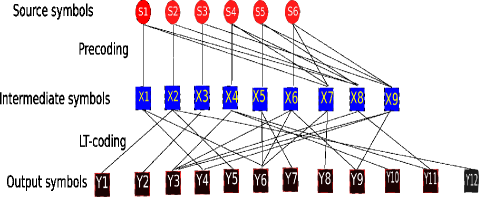
Refer to caption
Figure 1: Two-stage structure of a Raptor code with a sysmatic pre-code.

An illustration of a Raptor code is given in Figure 1. In this study, we assume that the pre-code is an (n,k)π‘›π‘˜(n,k) systematic LDPC code whose generator matrix, 𝐆nΓ—kpresuperscriptsubscriptπ†π‘›π‘˜pre\mathbf{G}_{n\times k}^{\textrm{pre}}, can always be written as 𝐆nΓ—kpre=[𝐈k|𝐏kΓ—(nβˆ’k)]Tsuperscriptsubscriptπ†π‘›π‘˜presuperscriptdelimited-[]conditionalsubscriptπˆπ‘˜subscriptππ‘˜π‘›π‘˜π‘‡\mathbf{G}_{n\times k}^{\textrm{pre}}=[\mathbf{I}_{k}|\mathbf{P}_{k\times(n-k)}]^{T}, where 𝐈ksubscriptπˆπ‘˜\mathbf{I}_{k} is an identity matrix of size kπ‘˜k, and 𝐏kΓ—(nβˆ’k)subscriptππ‘˜π‘›π‘˜\mathbf{P}_{k\times(n-k)} is a kπ‘˜k by (nβˆ’k)π‘›π‘˜(n-k) matrix with its entries being independent and identically distributed (i.i.d) Bernoulli random variables with parameter Ξ·πœ‚\eta. Such code is denoted as (n,k,Ξ·)π‘›π‘˜πœ‚(n,k,\eta) LDPC code [5]. Further, we can obtain the parity check matrix of this LDPC code as 𝐇(nβˆ’k)Γ—n=[𝐏(nβˆ’k)Γ—k|𝐈(nβˆ’k)](nβˆ’k)Γ—nsubscriptπ‡π‘›π‘˜π‘›subscriptdelimited-[]conditionalsubscriptππ‘›π‘˜π‘˜subscriptπˆπ‘›π‘˜π‘›π‘˜π‘›\mathbf{H}_{(n-k)\times n}=[\mathbf{P}_{(n-k)\times k}|\mathbf{I}_{(n-k)}]_{(n-k)\times n} and 𝐇(nβˆ’k)Γ—n×𝐆nΓ—kpre=𝟎subscriptπ‡π‘›π‘˜π‘›superscriptsubscriptπ†π‘›π‘˜pre0\mathbf{H}_{(n-k)\times n}\times\mathbf{G}_{n\times k}^{\textrm{pre}}=\mathbf{0}. In case where generator matrix of pre-code is a deterministic matrix, i.e., a typical (n,k)π‘›π‘˜(n,k) error correction code, there are well known methods to handle the situation and actually make our analysis easier.

When a coded packet is received by a MU, we use a 1Γ—k1π‘˜1\times k binary row vector 𝐠iLT​𝐆presuperscriptsubscript𝐠𝑖LTsuperscript𝐆pre\mathbf{g}_{i}^{\textrm{LT}}\mathbf{G}^{\textrm{pre}} to represent the coding information contained in the coded packet, where 𝐠iLTsuperscriptsubscript𝐠𝑖LT\mathbf{g}_{i}^{\textrm{LT}} is a 1Γ—n1𝑛1\times n binary row vector and 𝐆presuperscript𝐆pre\mathbf{G}^{\textrm{pre}} is a nΓ—kπ‘›π‘˜n\times k binary matrix. Let [𝐆]i,jsubscriptdelimited-[]𝐆𝑖𝑗\left[\mathbf{G}\right]_{i,j} denote the entry in the it​hsuperscriptπ‘–π‘‘β„Ži^{th} row and the jt​hsuperscriptπ‘—π‘‘β„Žj^{th} column of a matrix 𝐆𝐆\mathbf{G}. Particularly, [𝐠iL​T]1,jsubscriptdelimited-[]superscriptsubscript𝐠𝑖𝐿𝑇1𝑗\left[\mathbf{g}_{i}^{LT}\right]_{1,j} is 1 if the coded packet is a result of the XOR operation on the jt​hsuperscriptπ‘—π‘‘β„Žj^{th} intermediate packet (and other intermediate packets); otherwise [𝐠iL​T]1,jsubscriptdelimited-[]superscriptsubscript𝐠𝑖𝐿𝑇1𝑗\left[\mathbf{g}_{i}^{LT}\right]_{1,j} equals 0. For [𝐆pre]i,jsubscriptdelimited-[]superscript𝐆pre𝑖𝑗\left[\mathbf{G}^{\textrm{pre}}\right]_{i,j} , it is 1 if the it​hsuperscriptπ‘–π‘‘β„Ži^{th} intermediate packet is a result of the XOR operation on the jt​hsuperscriptπ‘—π‘‘β„Žj^{th} source packet (and other source packets); otherwise [𝐆pre]i,jsubscriptdelimited-[]superscript𝐆pre𝑖𝑗\left[\mathbf{G}^{\textrm{pre}}\right]_{i,j} equals 0. Therefore, a random row vector in this paper refers to the row vector of a randomly chosen coded packet where the coded packet is generated using the Raptor encoding process described above. Recall that 𝐬=(s1,s2,…,sk)𝐬subscript𝑠1subscript𝑠2…subscriptπ‘ π‘˜\mathbf{s}=\left(s_{1},s_{2},...,s_{k}\right) represents the kπ‘˜k equal-length source packets to be transmission. The coded packet can be expressed as: 𝐲i=𝐠iLT​𝐆pre​𝐬Tsubscript𝐲𝑖superscriptsubscript𝐠𝑖LTsuperscript𝐆presuperscript𝐬𝑇\mathbf{y}_{i}=\mathbf{g}_{i}^{\textrm{LT}}\mathbf{G}^{\textrm{pre}}\mathbf{s}^{T}, where β€œπ¬Tsuperscript𝐬𝑇\mathbf{s}^{T}” is transpose of 𝐬𝐬\mathbf{s}.

Raptor codes can be decoded by using a variety of decoding algorithms. A typically used decoding algorithm for Raptor Codes is the so-called β€œLT process” [4], but it is well known that the LT process is unable to decode all source packets which can be possibly recovered from information contained in the received coded packets. For example, LT process relies on the existence of at least one degree-one coded packet to be received in order to start the decoding process. For Raptor codes with limited lengths, i.e. on the order of a few thousand, maximum-likelihood (ML) decoding has been proposed to replace LT process. Therefore, in this paper we use a different decoding algorithm called the inactivation decoding algorithm [8] to decode the source packets. This decoding algorithm combines the optimality of Gaussian elimination with the efficiency of the β€œLT process” algorithm. Specifically, let mπ‘šm, (mβ‰₯k)π‘šπ‘˜(m\geq k), be the number of coded packets that have already been successfully received by a MU. The performance of inactivation algorithm is the same as Gaussian elimination. One way to apply Gaussian elimination on raptor code is to solve a system of linear equations given in the following [10].

(𝐆mΓ—nLT𝐇(nβˆ’k)Γ—n)​(𝐆nΓ—kpre​𝐬kΓ—1T)superscriptsubscriptπ†π‘šπ‘›LTsubscriptπ‡π‘›π‘˜π‘›superscriptsubscriptπ†π‘›π‘˜presuperscriptsubscriptπ¬π‘˜1𝑇\displaystyle\left(\begin{array}[t]{c}\mathbf{G}_{m\times n}^{\textrm{LT}}\\ \mathbf{H}_{(n-k)\times n}\end{array}\right)\left(\mathbf{G}_{n\times k}^{\textrm{pre}}\mathbf{s}_{k\times 1}^{T}\right) =\displaystyle= (𝐘mΓ—1𝟎(nβˆ’k)Γ—1)subscriptπ˜π‘š1subscript0π‘›π‘˜1\displaystyle\left(\begin{array}[t]{c}\mathbf{Y}_{m\times 1}\\ \mathbf{0}_{(n-k)\times 1}\end{array}\right)

where 𝐘mΓ—1=(𝐲1,𝐲2,…,𝐲m)Tsubscriptπ˜π‘š1superscriptsubscript𝐲1subscript𝐲2…subscriptπ²π‘šπ‘‡\mathbf{Y}_{m\times 1}=(\mathbf{y}_{1},\mathbf{y}_{2},...,\mathbf{y}_{m})^{T}. Additionally, we can obtain the following Lemma:

Lemma 1.

A MU can recover all kπ‘˜k source packets from the mπ‘šm coded packets using the inactivation decoding algorithm if and only if (𝐆LT;𝐇(nβˆ’k)Γ—n)(m+nβˆ’k)Γ—nsubscriptsuperscript𝐆LTsubscriptπ‡π‘›π‘˜π‘›π‘šπ‘›π‘˜π‘›(\mathbf{G}^{\textrm{LT}};\mathbf{H}_{(n-k)\times n})_{(m+n-k)\times n} is a full rank matrix, i.e. its rank equals n𝑛n, which is equivalent to the event that (𝐆LT​𝐆pre)mΓ—ksubscriptsuperscript𝐆LTsuperscript𝐆preπ‘šπ‘˜(\mathbf{G}^{\textrm{LT}}\mathbf{G}^{\textrm{pre}})_{m\times k} is a full rank matrix.

Proof:

The proof of this statement is provided in Appendix A. ∎

Note that in this paper, all algebraic operations and the associated analysis are conducted in a binary field. Obviously the event that (𝐆LT​𝐆pre)mΓ—ksubscriptsuperscript𝐆LTsuperscript𝐆preπ‘šπ‘˜(\mathbf{G}^{\textrm{LT}}\mathbf{G}^{\textrm{pre}})_{m\times k} is a full rank matrix is equivalent to the event Amksuperscriptsubscriptπ΄π‘šπ‘˜A_{m}^{k} that a MU can successfully decode all kπ‘˜k source packets using inactivation decoding algorithm provided the event that the MU has successfully received mπ‘šm coded packets. The main result of this paper is summarized in Theorems 2 and 3.

III Performance Analysis of Raptor Codes

Denote by Amksuperscriptsubscriptπ΄π‘šπ‘˜A_{m}^{k} the event that a receiver can successfully decode all kπ‘˜k source packets conditioned on the event that the receiver has successfully received mπ‘šm coded packets which is encoded with Raptor code from the BS. In this section, we shall analyze the probability of Amksuperscriptsubscriptπ΄π‘šπ‘˜A_{m}^{k}.

Because of the equivalence between the event Amksuperscriptsubscriptπ΄π‘šπ‘˜A_{m}^{k} and the event that (𝐆LT​𝐆pre)mΓ—ksubscriptsuperscript𝐆LTsuperscript𝐆preπ‘šπ‘˜(\mathbf{G}^{\textrm{LT}}\mathbf{G}^{\textrm{pre}})_{m\times k} is a full rank matrix, the analysis of Pr⁑(Amk)Prsuperscriptsubscriptπ΄π‘šπ‘˜\Pr\left(A_{m}^{k}\right) is conducted by analyzing the probability that the rank of (𝐆LT​𝐆pre)mΓ—ksubscriptsuperscript𝐆LTsuperscript𝐆preπ‘šπ‘˜(\mathbf{G}^{\textrm{LT}}\mathbf{G}^{\textrm{pre}})_{m\times k} is kπ‘˜k.

III-A Lower Bound on the Decoding Success Probability of Raptor Codes

In this subsection, we will derive a lower bound on the decoding success probability of Raptor codes with systematic pre-code, which is presented in the following theorem:

Theorem 2.

When the BS generates coded packets using the Raptor code (k,π’ž,Ω​(x))π‘˜π’žΞ©π‘₯(k,\mathcal{C},\Omega(x)) where π’žπ’ž\mathcal{C} is (n,k,Ξ·)π‘›π‘˜πœ‚(n,k,\eta) LDPC code and the coded packets received at a mobile user (MU) are decoded using the inactivation decoding algorithm, the probability that a MU can successfully decode all kπ‘˜k source packets from mπ‘šm received coded packets with mβ‰₯kπ‘šπ‘˜m\geq k , denoted by Pr⁑(Amk)Prsuperscriptsubscriptπ΄π‘šπ‘˜\Pr\left(A_{m}^{k}\right), is lower bounded by

Pr⁑(Amk)Prsuperscriptsubscriptπ΄π‘šπ‘˜\displaystyle\Pr\left(A_{m}^{k}\right) β‰₯\displaystyle\geq 1βˆ’βˆ‘i=1k()ikβˆ‘r=inβˆ’k+i(J(r))Dm(i,r)\displaystyle 1-\sum_{i=1}^{k}\left({}_{i}^{k}\right)\sum_{r=i}^{n-k+i}\left(J\left(r\right)\right){}^{m}D\left(i,r\right) (2)

where

J​(r)π½π‘Ÿ\displaystyle J(r) =\displaystyle= βˆ‘d=1nΞ©dβ€‹βˆ‘s=0,2,…,2β€‹βŒŠd2βŒ‹()sr()dβˆ’snβˆ’r()dn\displaystyle\sum_{d=1}^{n}\Omega_{d}\frac{\sum_{s=0,2,\ldots,2\left\lfloor\frac{d}{2}\right\rfloor}({}_{s}^{r})({}_{d-s}^{n-r})}{({}_{d}^{n})}

and

D​(i,r)π·π‘–π‘Ÿ\displaystyle D(i,r) =\displaystyle\!\!\!\!=\!\!\!\! ()rβˆ’inβˆ’k[1+(1βˆ’2Ξ·)i2]nβˆ’kβˆ’r+i\displaystyle\left({}_{r-i}^{n-k}\right)\left[\frac{1+(1-2\eta){}^{i}}{2}\right]^{n-k-r+i}
Γ—[1βˆ’(1βˆ’2Ξ·)i2]rβˆ’i\displaystyle\times\left[\frac{1-(1-2\eta){}^{i}}{2}\right]^{r-i}

and Ξ©dsubscriptΩ𝑑\Omega_{d} is the degree distribution of LT codes.

Proof:

Our proof relies on the use of the union bound of the independent events that vectors in the column vector space of 𝐆nΓ—kpresuperscriptsubscriptπ†π‘›π‘˜pre\mathbf{G}_{n\times k}^{\textrm{pre}} are in the null space of 𝐆mΓ—nLTsuperscriptsubscriptπ†π‘šπ‘›LT\mathbf{G}_{m\times n}^{\textrm{LT}}.

According to the property of the matrix product [11, Eq. (4.5.1)], we have

r​a​n​k​(𝐆mΓ—nLT​𝐆nΓ—kpre)π‘Ÿπ‘Žπ‘›π‘˜superscriptsubscriptπ†π‘šπ‘›LTsuperscriptsubscriptπ†π‘›π‘˜pre\displaystyle rank(\mathbf{G}_{m\times n}^{\textrm{LT}}\mathbf{G}_{n\times k}^{\textrm{pre}})
=\displaystyle\!\!\!\!\!\!=\!\!\!\!\!\! r​a​n​k​(𝐆nΓ—kpre)βˆ’dim{N​(𝐆mΓ—nLT)∩R​(𝐆nΓ—kpre)}π‘Ÿπ‘Žπ‘›π‘˜superscriptsubscriptπ†π‘›π‘˜predimension𝑁superscriptsubscriptπ†π‘šπ‘›LT𝑅superscriptsubscriptπ†π‘›π‘˜pre\displaystyle rank(\mathbf{G}_{n\times k}^{\textrm{pre}})-\dim\{N(\mathbf{G}_{m\times n}^{\textrm{LT}})\cap R(\mathbf{G}_{n\times k}^{\textrm{pre}})\}

where N​(βˆ™)π‘βˆ™N(\bullet) is the right-hand null space of a matrix, R​(βˆ™)π‘…βˆ™R(\bullet) is the column vector space generated by a matrix and dim{𝒱}dimension𝒱\dim\{\mathcal{V}\} represents number of vectors in any basis for a vector space 𝒱𝒱\mathcal{V}. It follows from the definition of 𝐆nΓ—kpresuperscriptsubscriptπ†π‘›π‘˜pre\mathbf{G}_{n\times k}^{\textrm{pre}} given earlier that the rank of 𝐆nΓ—kpresuperscriptsubscriptπ†π‘›π‘˜pre\mathbf{G}_{n\times k}^{\textrm{pre}} surely is kπ‘˜k. It can be readily obtained that:

Pr⁑[r​a​n​k​(𝐆mΓ—nLT​𝐆nΓ—kpre)=k]Prπ‘Ÿπ‘Žπ‘›π‘˜superscriptsubscriptπ†π‘šπ‘›LTsuperscriptsubscriptπ†π‘›π‘˜preπ‘˜\displaystyle\Pr[rank(\mathbf{G}_{m\times n}^{\textrm{LT}}\mathbf{G}_{n\times k}^{\textrm{pre}})=k] (3)
=\displaystyle= Pr⁑[dim{N​(𝐆mΓ—nLT)∩R​(𝐆nΓ—kpre)}=0]Prdimension𝑁superscriptsubscriptπ†π‘šπ‘›LT𝑅superscriptsubscriptπ†π‘›π‘˜pre0\displaystyle\Pr[\dim\{N(\mathbf{G}_{m\times n}^{\textrm{LT}})\cap R(\mathbf{G}_{n\times k}^{\textrm{pre}})\}=0]

For convenience let Wm,n,ksubscriptπ‘Šπ‘šπ‘›π‘˜W_{m,n,k} represent the event that dim{N​(𝐆mΓ—nLT)∩R​(𝐆nΓ—kpre)}=0dimension𝑁superscriptsubscriptπ†π‘šπ‘›LT𝑅superscriptsubscriptπ†π‘›π‘˜pre0\dim\{N(\mathbf{G}_{m\times n}^{\textrm{LT}})\cap R(\mathbf{G}_{n\times k}^{\textrm{pre}})\}=0. Now we need to analyze Pr⁑[Wm,n,k]Prsubscriptπ‘Šπ‘šπ‘›π‘˜\Pr[W_{m,n,k}]. Provided that 𝐆nΓ—kpresuperscriptsubscriptπ†π‘›π‘˜pre\mathbf{G}_{n\times k}^{\textrm{pre}} is a (n,k,ρ)π‘›π‘˜πœŒ(n,k,\rho) systematic LDPC code, the event dim{N​(𝐆mΓ—nLT)∩R​(𝐆nΓ—kpre)}β‰ 0dimension𝑁superscriptsubscriptπ†π‘šπ‘›LT𝑅superscriptsubscriptπ†π‘›π‘˜pre0\dim\{N(\mathbf{G}_{m\times n}^{\textrm{LT}})\cap R(\mathbf{G}_{n\times k}^{\textrm{pre}})\}\neq 0, i.e., WΒ―m,n,ksubscriptΒ―π‘Šπ‘šπ‘›π‘˜\overline{W}_{m,n,k}, is equivalent to the event that at least one column vector from R​(𝐆nΓ—kpre)𝑅superscriptsubscriptπ†π‘›π‘˜preR(\mathbf{G}_{n\times k}^{\textrm{pre}}) is among N​(𝐆mΓ—nL​T)𝑁superscriptsubscriptπ†π‘šπ‘›πΏπ‘‡N(\mathbf{G}_{m\times n}^{LT}), i.e., βˆͺ𝐱∈R​(𝐆nΓ—kpre)𝐆mΓ—nLT​𝐱=𝟎subscript𝐱𝑅superscriptsubscriptπ†π‘›π‘˜presuperscriptsubscriptπ†π‘šπ‘›LT𝐱0\cup_{\mathbf{x}\in R(\mathbf{G}_{n\times k}^{\textrm{pre}})}\mathbf{G}_{m\times n}^{\textrm{LT}}\mathbf{x}=\mathbf{0}, where 𝐱𝐱\mathbf{x} is a column vector of R​(𝐆nΓ—kpre)𝑅superscriptsubscriptπ†π‘›π‘˜preR(\mathbf{G}_{n\times k}^{\textrm{pre}}). It can be readily shown that:

Pr⁑[WΒ―m,n,k]PrsubscriptΒ―π‘Šπ‘šπ‘›π‘˜\displaystyle\Pr[\overline{W}_{m,n,k}] =\displaystyle= Pr⁑[βˆͺ𝐱∈R​(𝐆nΓ—kpre)𝐆mΓ—nLT​𝐱=𝟎]Prsubscript𝐱𝑅superscriptsubscriptπ†π‘›π‘˜presuperscriptsubscriptπ†π‘šπ‘›LT𝐱0\displaystyle\Pr\left[\cup_{\mathbf{x}\in R(\mathbf{G}_{n\times k}^{\textrm{pre}})}\mathbf{G}_{m\times n}^{\textrm{LT}}\mathbf{x}=\mathbf{0}\right] (4)
≀\displaystyle\leq βˆ‘π±βˆˆR​(𝐆nΓ—kpre)Pr⁑[𝐆mΓ—nLT​𝐱=𝟎]subscript𝐱𝑅superscriptsubscriptπ†π‘›π‘˜prePrsuperscriptsubscriptπ†π‘šπ‘›LT𝐱0\displaystyle\sum_{\mathbf{x}\in R(\mathbf{G}_{n\times k}^{\textrm{pre}})}\Pr\left[\mathbf{G}_{m\times n}^{\textrm{LT}}\mathbf{x}=\mathbf{0}\right]

The column vector space R​(𝐆nΓ—kpre)𝑅superscriptsubscriptπ†π‘›π‘˜preR(\mathbf{G}_{n\times k}^{\textrm{pre}}) is partitioned into kπ‘˜k subspace (𝒱1,𝒱2,…,𝒱k)subscript𝒱1subscript𝒱2…subscriptπ’±π‘˜(\mathcal{V}_{1},\mathcal{V}_{2},\ldots,\mathcal{V}_{k}) and 𝒱isubscript𝒱𝑖\mathcal{V}_{i} is the subspace that contains all the column vectors which are summation of i𝑖i column vectors of 𝐆nΓ—kpresuperscriptsubscriptπ†π‘›π‘˜pre\mathbf{G}_{n\times k}^{\textrm{pre}}. We denote Ξ“isubscriptΓ𝑖\text{\leavevmode{G}}_{i} as the set of indices of the column vectors in 𝒱isubscript𝒱𝑖\mathcal{V}_{i} and there are (ik)(_{i}^{k}) indices in Ξ“isubscriptΓ𝑖\text{\leavevmode{G}}_{i}. Let 𝐱aisuperscriptsubscriptπ±π‘Žπ‘–\mathbf{x}_{a}^{i} represent the at​h,aβˆˆΞ“isuperscriptπ‘Žπ‘‘β„Žπ‘ŽsubscriptΓ𝑖a^{th},a\in\text{\leavevmode{G}}_{i} column vector in 𝒱isubscript𝒱𝑖\mathcal{V}_{i}. It can be readily shown that:

βˆ‘π±βˆˆR​(𝐆nΓ—kpre)Pr⁑[𝐆mΓ—nLT​𝐱=𝟎]subscript𝐱𝑅superscriptsubscriptπ†π‘›π‘˜prePrsuperscriptsubscriptπ†π‘šπ‘›LT𝐱0\displaystyle\!\!\!\!\sum_{\mathbf{x}\in R(\mathbf{G}_{n\times k}^{\textrm{pre}})}\!\!\!\!\Pr[\mathbf{G}_{m\times n}^{\textrm{LT}}\mathbf{x}=\mathbf{0}] =\displaystyle\!\!\!\!=\!\!\!\! βˆ‘i=1kβˆ‘aβˆˆΞ“iPr⁑[𝐆mΓ—nLT​𝐱ai=𝟎]superscriptsubscript𝑖1π‘˜subscriptπ‘ŽsubscriptΓ𝑖Prsuperscriptsubscriptπ†π‘šπ‘›LTsuperscriptsubscriptπ±π‘Žπ‘–0\displaystyle\sum_{i=1}^{k}\sum_{a\in\text{\leavevmode{G}}_{i}}\Pr[\mathbf{G}_{m\times n}^{\textrm{LT}}\mathbf{x}_{a}^{i}=\mathbf{0}] (5)

We can observe that 𝐱ai=𝐆nΓ—iaβ€‹πŸisuperscriptsubscriptπ±π‘Žπ‘–superscriptsubscriptπ†π‘›π‘–π‘Žsubscript1𝑖\mathbf{x}_{a}^{i}=\mathbf{G}_{n\times i}^{a}\mathbf{1}_{i} where 𝐆nΓ—iasuperscriptsubscriptπ†π‘›π‘–π‘Ž\mathbf{G}_{n\times i}^{a} is the matrix formed by i𝑖i selected column vectors from kπ‘˜k column vectors of 𝐆nΓ—kpresuperscriptsubscriptπ†π‘›π‘˜pre\mathbf{G}_{n\times k}^{\textrm{pre}} and 𝟏isubscript1𝑖\mathbf{1}_{i} represent the iΓ—1𝑖1i\times 1 all one column vector. Let |𝐱ai|superscriptsubscriptπ±π‘Žπ‘–\left|\mathbf{x}_{a}^{i}\right| represent the weight of column vector 𝐱aisuperscriptsubscriptπ±π‘Žπ‘–\mathbf{x}_{a}^{i}, considering the law of total probability, we have

Pr⁑[𝐆mΓ—nLT​𝐱ai=𝟎]Prsuperscriptsubscriptπ†π‘šπ‘›LTsuperscriptsubscriptπ±π‘Žπ‘–0\displaystyle\Pr[\mathbf{G}_{m\times n}^{\textrm{LT}}\mathbf{x}_{a}^{i}=\mathbf{0}] (6)
=\displaystyle= βˆ‘r=0nPr[𝐆mΓ—nLT𝐱ai=𝟎||𝐱ai|=r]Pr[|𝐱ai|=r]\displaystyle\sum_{r=0}^{n}\Pr\left[\mathbf{G}_{m\times n}^{\textrm{LT}}\mathbf{x}_{a}^{i}=\mathbf{0}\Bigr{|}\left|\mathbf{x}_{a}^{i}\right|=r\right]\Pr\left[\left|\mathbf{x}_{a}^{i}\right|=r\right]

Firstly, we need to calculate Pr⁑[|𝐱ai|=r]Prsuperscriptsubscriptπ±π‘Žπ‘–π‘Ÿ\Pr\left[\left|\mathbf{x}_{a}^{i}\right|=r\right]. Provided 𝐆nΓ—kpre=[𝐈k|𝐏kΓ—(nβˆ’k)]Tsuperscriptsubscriptπ†π‘›π‘˜presuperscriptdelimited-[]conditionalsubscriptπˆπ‘˜subscriptππ‘˜π‘›π‘˜π‘‡\mathbf{G}_{n\times k}^{\textrm{pre}}=[\mathbf{I}_{k}|\mathbf{P}_{k\times(n-k)}]^{T}, in the first kπ‘˜k entries of 𝐆nΓ—iaβ€‹πŸisuperscriptsubscriptπ†π‘›π‘–π‘Žsubscript1𝑖\mathbf{G}_{n\times i}^{a}\mathbf{1}_{i} there are i𝑖i ones. If |𝐱ai|=rsuperscriptsubscriptπ±π‘Žπ‘–π‘Ÿ\left|\mathbf{x}_{a}^{i}\right|=r, then there are rβˆ’iπ‘Ÿπ‘–r-i ones in the last nβˆ’kπ‘›π‘˜n-k entries of 𝐆nΓ—iaβ€‹πŸisuperscriptsubscriptπ†π‘›π‘–π‘Žsubscript1𝑖\mathbf{G}_{n\times i}^{a}\mathbf{1}_{i}, .i.e, 𝐏(nβˆ’k)Γ—iaβ€‹πŸisuperscriptsubscriptππ‘›π‘˜π‘–π‘Žsubscript1𝑖\mathbf{P}_{(n-k)\times i}^{a}\mathbf{1}_{i}. Hence we can obtain that

Pr⁑[|𝐱ai|=r]Prsuperscriptsubscriptπ±π‘Žπ‘–π‘Ÿ\displaystyle\Pr\left[\left|\mathbf{x}_{a}^{i}\right|=r\right] =\displaystyle= Pr⁑[|𝐏(nβˆ’k)Γ—iaβ€‹πŸi|=(rβˆ’i)]Prsuperscriptsubscriptππ‘›π‘˜π‘–π‘Žsubscript1π‘–π‘Ÿπ‘–\displaystyle\Pr\left[\left|\mathbf{P}_{(n-k)\times i}^{a}\mathbf{1}_{i}\right|=(r-i)\right] (7)

and i≀r≀nβˆ’k+iπ‘–π‘Ÿπ‘›π‘˜π‘–i\leq r\leq n-k+i. The rows of 𝐏(nβˆ’k)Γ—iasuperscriptsubscriptππ‘›π‘˜π‘–π‘Ž\mathbf{P}_{(n-k)\times i}^{a}, i.e., 𝐩j,1≀j≀(nβˆ’k)subscript𝐩𝑗1π‘—π‘›π‘˜\mathbf{p}_{j},1\leq j\leq(n-k), are random binary row vectors, which are generated independently. Each entry of 𝐏(nβˆ’k)Γ—iasuperscriptsubscriptππ‘›π‘˜π‘–π‘Ž\mathbf{P}_{(n-k)\times i}^{a} is independent and identically distributed (i.i.d) Bernoulli random variable with parameter ρ𝜌\rho. Therefore, Pr⁑[𝐩jβ€‹πŸi=0]=Pr⁑[𝐩k,kβ‰ jβ€‹πŸi=0]Prsubscript𝐩𝑗subscript1𝑖0Prsubscriptπ©π‘˜π‘˜π‘—subscript1𝑖0\Pr[\mathbf{p}_{j}\mathbf{1}_{i}=0]=\Pr[\mathbf{p}_{k,k\neq j}\mathbf{1}_{i}=0]. The event that the jt​hsuperscriptπ‘—π‘‘β„Žj^{th} entry in 𝐱aisuperscriptsubscriptπ±π‘Žπ‘–\mathbf{x}_{a}^{i} is zero is equivalent to the event that there are even number of ones in row vector 𝐩jsubscript𝐩𝑗\mathbf{p}_{j}. We have

Pr⁑[𝐩jβ€‹πŸi=0]Prsubscript𝐩𝑗subscript1𝑖0\displaystyle\Pr[\mathbf{p}_{j}\mathbf{1}_{i}=0] =\displaystyle= Pr⁑[|𝐩j|​ is evenΒ ]Prsubscript𝐩𝑗 is evenΒ \displaystyle\Pr\left[\left|\mathbf{p}_{j}\right|\textrm{ is even }\right] (8)
=\displaystyle= βˆ‘s=0,2,…,2β€‹βŒŠi2βŒ‹()siΞ·s(1βˆ’Ξ·)(iβˆ’s)\displaystyle\sum_{s=0,2,\ldots,2\left\lfloor\frac{i}{2}\right\rfloor}({}_{s}^{i})\eta^{s}(1-\eta)^{(i-s)}
=\displaystyle= [(Ξ·+(1βˆ’Ξ·))i+(βˆ’Ξ·+(1βˆ’Ξ·))i]2delimited-[]superscriptπœ‚1πœ‚π‘–superscriptπœ‚1πœ‚π‘–2\displaystyle\frac{[(\eta+(1-\eta))^{i}+(-\eta+(1-\eta))^{i}]}{2}
=\displaystyle= 1+(1βˆ’2Ξ·)i2\displaystyle\frac{1+(1-2\eta){}^{i}}{2}

There are ()rβˆ’inβˆ’k({}_{r-i}^{n-k}) possible combination for rβˆ’iπ‘Ÿπ‘–r-i ones in the last nβˆ’kπ‘›π‘˜n-k entries. It can be readily shown that:

Pr⁑[|𝐏(nβˆ’k)Γ—iaβ€‹πŸi|=(rβˆ’i)]Prsuperscriptsubscriptππ‘›π‘˜π‘–π‘Žsubscript1π‘–π‘Ÿπ‘–\displaystyle\Pr\left[\left|\mathbf{P}_{(n-k)\times i}^{a}\mathbf{1}_{i}\right|=(r-i)\right] (9)
=\displaystyle= ()rβˆ’inβˆ’k{Pr[𝐩j𝟏i=0]}nβˆ’kβˆ’r+i\displaystyle({}_{r-i}^{n-k})\{\Pr[\mathbf{p}_{j}\mathbf{1}_{i}=0]\}^{n-k-r+i}
Γ—{1βˆ’Pr⁑[𝐩jβ€‹πŸi=0]}rβˆ’iabsentsuperscript1Prsubscript𝐩𝑗subscript1𝑖0π‘Ÿπ‘–\displaystyle\times\{1-\Pr[\mathbf{p}_{j}\mathbf{1}_{i}=0]\}^{r-i}

Combining equations (7), (8) and (9), we can obtain that

D​(i,r)=Pr⁑[|𝐱ai|=r]π·π‘–π‘ŸPrsuperscriptsubscriptπ±π‘Žπ‘–π‘Ÿ\displaystyle D(i,r)=\Pr\left[\left|\mathbf{x}_{a}^{i}\right|=r\right] (10)
=\displaystyle= ()rβˆ’inβˆ’k[1+(1βˆ’2Ξ·)i2]nβˆ’kβˆ’r+i\displaystyle\left({}_{r-i}^{n-k}\right)\left[\frac{1+(1-2\eta){}^{i}}{2}\right]^{n-k-r+i}
Γ—[1βˆ’(1βˆ’2Ξ·)i2]rβˆ’i\displaystyle\times\left[\frac{1-(1-2\eta){}^{i}}{2}\right]^{r-i}

For 𝐱ai,𝐱b,bβ‰ aiβˆˆπ’±isuperscriptsubscriptπ±π‘Žπ‘–superscriptsubscriptπ±π‘π‘π‘Žπ‘–subscript𝒱𝑖\mathbf{x}_{a}^{i},\mathbf{x}_{b,b\neq a}^{i}\in\mathcal{V}_{i}, 𝐏(nβˆ’k)Γ—iasuperscriptsubscriptππ‘›π‘˜π‘–π‘Ž\mathbf{P}_{(n-k)\times i}^{a} and 𝐏(nβˆ’k)Γ—ibsuperscriptsubscriptππ‘›π‘˜π‘–π‘\mathbf{P}_{(n-k)\times i}^{b} have the same probability to form the same matrix formation. So we can obtain that Pr⁑[|𝐏(nβˆ’k)Γ—iaβ€‹πŸi|=(rβˆ’i)]=Pr⁑[|𝐏(nβˆ’k)Γ—ibβ€‹πŸi|=(rβˆ’i)]Prsuperscriptsubscriptππ‘›π‘˜π‘–π‘Žsubscript1π‘–π‘Ÿπ‘–Prsuperscriptsubscriptππ‘›π‘˜π‘–π‘subscript1π‘–π‘Ÿπ‘–\Pr\left[\left|\mathbf{P}_{(n-k)\times i}^{a}\mathbf{1}_{i}\right|=(r-i)\right]=\Pr\left[\left|\mathbf{P}_{(n-k)\times i}^{b}\mathbf{1}_{i}\right|=(r-i)\right], in turn Pr⁑[|𝐱ai|=r]=Pr⁑[|𝐱bi|=r]Prsuperscriptsubscriptπ±π‘Žπ‘–π‘ŸPrsuperscriptsubscriptπ±π‘π‘–π‘Ÿ\Pr\left[\left|\mathbf{x}_{a}^{i}\right|=r\right]=\Pr\left[\left|\mathbf{x}_{b}^{i}\right|=r\right]. Now, we calculate Pr⁑[𝐆mΓ—nL​T​𝐱ai=0∣|𝐱ai|=r]Prsuperscriptsubscriptπ†π‘šπ‘›πΏπ‘‡superscriptsubscriptπ±π‘Žπ‘–0superscriptsubscriptπ±π‘Žπ‘–π‘Ÿ\Pr\left[\mathbf{G}_{m\times n}^{LT}\mathbf{x}_{a}^{i}=0\mid\left|\mathbf{x}_{a}^{i}\right|=r\right]. The rows of 𝐆mΓ—nLTsuperscriptsubscriptπ†π‘šπ‘›LT\mathbf{G}_{m\times n}^{\textrm{LT}}, i.e., 𝐠jLT,1≀j≀msuperscriptsubscript𝐠𝑗LT1π‘—π‘š\mathbf{g}_{j}^{\textrm{LT}},1\leq j\leq m, are random binary row vectors, which are generated independently. We have

Pr[𝐆mΓ—nLT𝐱ai=𝟎||𝐱ai|=r]\displaystyle\Pr\left[\mathbf{G}_{m\times n}^{\textrm{LT}}\mathbf{x}_{a}^{i}=\mathbf{0}\Bigr{|}\left|\mathbf{x}_{a}^{i}\right|=r\right] (11)
=\displaystyle\!\!\!\!\!\!=\!\!\!\!\!\! {Pr[𝐠jLT𝐱ai=0||𝐱ai|=r]}m\displaystyle\left\{\Pr\left[\mathbf{g}_{j}^{\textrm{LT}}\mathbf{x}_{a}^{i}=0\Bigr{|}\left|\mathbf{x}_{a}^{i}\right|=r\right]\right\}^{m}

The degree of 𝐠jLTsuperscriptsubscript𝐠𝑗LT\mathbf{g}_{j}^{\textrm{LT}}, i.e. the number of non-zero elements of 𝐠jLTsuperscriptsubscript𝐠𝑗LT\mathbf{g}_{j}^{\textrm{LT}}, is chosen according to the pre-defined degree distribution 𝛀=(Ξ©1,…,Ξ©n)𝛀subscriptΞ©1…subscriptΩ𝑛\mathbf{\Omega}=(\Omega_{1},...,\Omega_{n}) and each non-zero element is then placed randomly and uniformly into 𝐠jLTsuperscriptsubscript𝐠𝑗LT\mathbf{g}_{j}^{\textrm{LT}}. It can be readily obtain that

Pr[𝐠jLT𝐱ai=0||𝐱ai|=r]\displaystyle\Pr\left[\mathbf{g}_{j}^{\textrm{LT}}\mathbf{x}_{a}^{i}=0\Bigr{|}\left|\mathbf{x}_{a}^{i}\right|=r\right] (12)
=\displaystyle= βˆ‘d=1nΞ©dPr[𝐠jLT𝐱ai=0||𝐱ai|=r,|𝐠jLT|=d]\displaystyle\sum_{d=1}^{n}\Omega_{d}\Pr\left[\mathbf{g}_{j}^{\textrm{LT}}\mathbf{x}_{a}^{i}=0\Bigr{|}\left|\mathbf{x}_{a}^{i}\right|=r,\left|\mathbf{g}_{j}^{\textrm{LT}}\right|=d\right]

Let 𝐫ji=(𝐠j​1LT​𝐱a​1i,𝐠j​2LT​𝐱a​2i,…,𝐠j​nLT​𝐱a​ni)superscriptsubscript𝐫𝑗𝑖superscriptsubscript𝐠𝑗1LTsuperscriptsubscriptπ±π‘Ž1𝑖superscriptsubscript𝐠𝑗2LTsuperscriptsubscriptπ±π‘Ž2𝑖…superscriptsubscript𝐠𝑗𝑛LTsuperscriptsubscriptπ±π‘Žπ‘›π‘–\mathbf{r}_{j}^{i}=(\mathbf{g}_{j1}^{\textrm{LT}}\mathbf{x}_{a1}^{i},\mathbf{g}_{j2}^{\textrm{LT}}\mathbf{x}_{a2}^{i},...,\mathbf{g}_{jn}^{\textrm{LT}}\mathbf{x}_{an}^{i}), where 𝐠j​kLTsuperscriptsubscriptπ π‘—π‘˜LT\mathbf{g}_{jk}^{\textrm{LT}} is [𝐠jLT]1,ksubscriptdelimited-[]superscriptsubscript𝐠𝑗LT1π‘˜\left[\mathbf{g}_{j}^{\textrm{LT}}\right]_{1,k} and 𝐱a​kisuperscriptsubscriptπ±π‘Žπ‘˜π‘–\mathbf{x}_{ak}^{i} is [𝐱ai]k,1subscriptdelimited-[]superscriptsubscriptπ±π‘Žπ‘–π‘˜1\left[\mathbf{x}_{a}^{i}\right]_{k,1}. Then, we can obtain that

Pr[𝐠jLT𝐱ai=0||𝐱ai|=r,|𝐠jLT|=d]\displaystyle\Pr\left[\mathbf{g}_{j}^{\textrm{LT}}\mathbf{x}_{a}^{i}=0\Bigr{|}\left|\mathbf{x}_{a}^{i}\right|=r,\left|\mathbf{g}_{j}^{\textrm{LT}}\right|=d\right] (13)
=\displaystyle= Pr[|𝐫ji| is even ||𝐱ai|=r,|𝐠jLT|=d]\displaystyle\Pr\left[\left|\mathbf{r}_{j}^{i}\right|\textrm{ is even }\Bigr{|}\left|\mathbf{x}_{a}^{i}\right|=r,\left|\mathbf{g}_{j}^{\textrm{LT}}\right|=d\right]
=\displaystyle= βˆ‘s=0,2,…,2β€‹βŒŠd2βŒ‹()sr()dβˆ’snβˆ’r()dn\displaystyle\frac{\sum_{s=0,2,\ldots,2\left\lfloor\frac{d}{2}\right\rfloor}({}_{s}^{r})({}_{d-s}^{n-r})}{({}_{d}^{n})}

Combining equations (12) and (13), we can obtain that

J​(r)π½π‘Ÿ\displaystyle J(r) =\displaystyle= Pr[𝐠jLT𝐱ai=0||𝐱ai|=r]\displaystyle\Pr\left[\mathbf{g}_{j}^{\textrm{LT}}\mathbf{x}_{a}^{i}=0\Bigr{|}\left|\mathbf{x}_{a}^{i}\right|=r\right] (14)
=\displaystyle= βˆ‘d=1nΞ©dβ€‹βˆ‘s=0,2,…,2β€‹βŒŠd2βŒ‹()sr()dβˆ’snβˆ’r()dn\displaystyle\sum_{d=1}^{n}\Omega_{d}\frac{\sum_{s=0,2,\ldots,2\left\lfloor\frac{d}{2}\right\rfloor}({}_{s}^{r})({}_{d-s}^{n-r})}{({}_{d}^{n})}

Inserting equation (11) into (14), it can be obtained that

Pr[𝐆mΓ—nLT𝐱ai=𝟎||𝐱ai|=r]\displaystyle\Pr\left[\mathbf{G}_{m\times n}^{\textrm{LT}}\mathbf{x}_{a}^{i}=\mathbf{0}\Bigr{|}\left|\mathbf{x}_{a}^{i}\right|=r\right] =\displaystyle= [J​(r)]msuperscriptdelimited-[]π½π‘Ÿπ‘š\displaystyle\left[J(r)\right]^{m} (15)

We can obtain that Pr⁑[𝐆mΓ—nLT​𝐱ai=𝟎∣|𝐱ai|=r]Prsuperscriptsubscriptπ†π‘šπ‘›LTsuperscriptsubscriptπ±π‘Žπ‘–0superscriptsubscriptπ±π‘Žπ‘–π‘Ÿ\Pr[\mathbf{G}_{m\times n}^{\textrm{LT}}\mathbf{x}_{a}^{i}=\mathbf{0}\mid\left|\mathbf{x}_{a}^{i}\right|=r] is only determined by the weight of 𝐱aisuperscriptsubscriptπ±π‘Žπ‘–\mathbf{x}_{a}^{i} rather than which i𝑖i column vectors is chosen from 𝐆nΓ—kpresuperscriptsubscriptπ†π‘›π‘˜pre\mathbf{G}_{n\times k}^{\textrm{pre}} to obtain the summation 𝐱aisuperscriptsubscriptπ±π‘Žπ‘–\mathbf{x}_{a}^{i}. So we can conclude that Pr⁑[𝐆mΓ—nLT​𝐱ai=𝟎]=Pr⁑[𝐆mΓ—nLT​𝐱bi=𝟎]Prsuperscriptsubscriptπ†π‘šπ‘›LTsuperscriptsubscriptπ±π‘Žπ‘–0Prsuperscriptsubscriptπ†π‘šπ‘›LTsuperscriptsubscript𝐱𝑏𝑖0\Pr[\mathbf{G}_{m\times n}^{\textrm{LT}}\mathbf{x}_{a}^{i}=\mathbf{0}]=\Pr[\mathbf{G}_{m\times n}^{\textrm{LT}}\mathbf{x}_{b}^{i}=\mathbf{0}]. Recall that there are (ik)(_{i}^{k}) indices in Ξ“isubscriptΓ𝑖\text{\leavevmode{G}}_{i}. Inserting equations (10) and (15) into (6) and combining with equation (5), yields the following results

Pr⁑[WΒ―m,n,k]PrsubscriptΒ―π‘Šπ‘šπ‘›π‘˜\displaystyle\Pr[\overline{W}_{m,n,k}] (16)
≀\displaystyle\leq βˆ‘i=1kβˆ‘aβˆˆΞ“iPr⁑[𝐆mΓ—nLT​𝐱ai=𝟎]superscriptsubscript𝑖1π‘˜subscriptπ‘ŽsubscriptΓ𝑖Prsuperscriptsubscriptπ†π‘šπ‘›LTsuperscriptsubscriptπ±π‘Žπ‘–0\displaystyle\sum_{i=1}^{k}\sum_{a\in\text{\leavevmode{G}}_{i}}\Pr\left[\mathbf{G}_{m\times n}^{\textrm{LT}}\mathbf{x}_{a}^{i}=\mathbf{0}\right]
=\displaystyle= βˆ‘i=1k()ikβˆ‘r=inβˆ’k+i[βˆ‘d=1nΞ©dβˆ‘s=0,2,…,2β€‹βŒŠd2βŒ‹()sr()dβˆ’snβˆ’r()dn]m\displaystyle\sum_{i=1}^{k}({}_{i}^{k})\sum_{r=i}^{n-k+i}\left[\sum_{d=1}^{n}\Omega_{d}\frac{\sum_{s=0,2,\ldots,2\left\lfloor\frac{d}{2}\right\rfloor}({}_{s}^{r})({}_{d-s}^{n-r})}{({}_{d}^{n})}\right]^{m}
Γ—()rβˆ’inβˆ’k[1+(1βˆ’2Ξ·)i2]nβˆ’kβˆ’r+i[1βˆ’(1βˆ’2Ξ·)i2]rβˆ’i\displaystyle\times\left({}_{r-i}^{n-k}\right)\left[\frac{1+(1-2\eta){}^{i}}{2}\right]^{n-k-r+i}\left[\frac{1-(1-2\eta){}^{i}}{2}\right]^{r-i}

which proves the assertion. ∎

III-B Upper Bound on the Decoding Success Probability of Raptor Codes

In addition to the above lower bound, we can also derive an upper bound on the decoding success probability of Raptor codes with systematic pre-code, which is presented in the following theorem:

Theorem 3.

When the BS generates coded packets using the Raptor code (k,π’ž,Ω​(x))π‘˜π’žΞ©π‘₯(k,\mathcal{C},\Omega(x)) and the coded packets received at a mobile user (MU) are decoded using the inactivation decoding algorithm, the probability that a MU can successfully decode all kπ‘˜k source packets from mπ‘šm received coded packets with mβ‰₯kπ‘šπ‘˜m\geq k , denoted by Pr⁑(Amk)Prsuperscriptsubscriptπ΄π‘šπ‘˜\Pr\left(A_{m}^{k}\right), is upper bounded by:

Pr⁑(Amk)Prsuperscriptsubscriptπ΄π‘šπ‘˜\displaystyle\Pr\left(A_{m}^{k}\right) (17)
≀\displaystyle\!\!\!\!\leq\!\!\!\! 1βˆ’βˆ‘i=1k()ikβˆ‘r=inβˆ’k+i(J(r))mD(i,r)\displaystyle 1-\sum_{i=1}^{k}({}_{i}^{k})\sum_{r=i}^{n-k+i}(J(r))^{m}D(i,r)
+12βˆ‘i=1k()ikβˆ‘w0=0iβˆ‘w1=iβˆ’w0βˆ‘w2=0kβˆ’i𝟏(w0+w2)𝟏(w1+w2)\displaystyle+\frac{1}{2}\sum_{i=1}^{k}({}_{i}^{k})\sum_{w_{0}=0}^{i}\sum_{w_{1}=i-w_{0}}\sum_{w_{2}=0}^{k-i}\mathbf{1}(w_{0}+w_{2})\mathbf{1}(w_{1}+w_{2})
Γ—\displaystyle\times\!\!\!\! ()w0i()w2kβˆ’iβˆ‘r0=w0nβˆ’k+w0βˆ‘r1=w1nβˆ’k+w1βˆ‘r0=w2nβˆ’k+w2D(w0,r0)D(w1,r1)\displaystyle({}_{w_{0}}^{i})({}_{w_{2}}^{k-i})\sum_{r_{0}=w_{0}}^{n-k+w_{0}}\sum_{r_{1}=w_{1}}^{n-k+w_{1}}\sum_{r_{0}=w_{2}}^{n-k+w_{2}}D(w_{0},r_{0})D(w_{1},r_{1})
Γ—\displaystyle\times\!\!\!\! D​(w2,r2)​{J​(r0)​J​(r1)​J​(r2)+J¯​(r0)​J¯​(r1)​J¯​(r2)}m𝐷subscript𝑀2subscriptπ‘Ÿ2superscript𝐽subscriptπ‘Ÿ0𝐽subscriptπ‘Ÿ1𝐽subscriptπ‘Ÿ2¯𝐽subscriptπ‘Ÿ0¯𝐽subscriptπ‘Ÿ1¯𝐽subscriptπ‘Ÿ2π‘š\displaystyle D(w_{2},r_{2})\{J(r_{0})J(r_{1})J(r_{2})+\overline{J}(r_{0})\overline{J}(r_{1})\overline{J}(r_{2})\}^{m}

where

πŸβ€‹(x)1π‘₯\displaystyle\mathbf{1}(x) :=assign\displaystyle:= {0if ​x=01o​t​h​e​r​w​i​s​ecases0ifΒ π‘₯01π‘œπ‘‘β„Žπ‘’π‘Ÿπ‘€π‘–π‘ π‘’\displaystyle\begin{cases}0&\textrm{if }x=0\\ 1&otherwise\end{cases}

J¯​(β‹…)=1βˆ’J​(β‹…)¯𝐽⋅1𝐽⋅\overline{J}(\cdot)=1-J(\cdot), D​(w0,r0)𝐷subscript𝑀0subscriptπ‘Ÿ0D(w_{0},r_{0}) is defined in equation (10) and J​(r0)𝐽subscriptπ‘Ÿ0J(r_{0}) is defined in equation (14).

Proof:

By using the Bonferroni inequality [Commtet1974Adv], we can obtain a lower bound of Pr⁑[WΒ―m,n,k]PrsubscriptΒ―π‘Šπ‘šπ‘›π‘˜\Pr[\overline{W}_{m,n,k}] as:

Pr⁑[WΒ―m,n,k]PrsubscriptΒ―π‘Šπ‘šπ‘›π‘˜\displaystyle\Pr[\overline{W}_{m,n,k}] (18)
=\displaystyle\!\!\!\!\!\!\!\!=\!\!\!\! Pr⁑[βˆͺ𝐱∈R​(𝐆nΓ—kpre)𝐆mΓ—nLT​𝐱=𝟎]Prsubscript𝐱𝑅superscriptsubscriptπ†π‘›π‘˜presuperscriptsubscriptπ†π‘šπ‘›LT𝐱0\displaystyle\Pr[\cup_{\mathbf{x}\in R(\mathbf{G}_{n\times k}^{\textrm{pre}})}\mathbf{G}_{m\times n}^{\textrm{LT}}\mathbf{x}=\mathbf{0}]
β‰₯(a)superscriptπ‘Ž\displaystyle\!\!\!\!\!\!\!\!\stackrel{{\scriptstyle(a)}}{{\geq}}\!\!\!\! βˆ‘π±βˆˆR​(𝐆nΓ—kpre)Pr⁑[𝐆mΓ—nLT​𝐱=𝟎]subscript𝐱𝑅superscriptsubscriptπ†π‘›π‘˜prePrsuperscriptsubscriptπ†π‘šπ‘›LT𝐱0\displaystyle\sum_{\mathbf{x}\in R(\mathbf{G}_{n\times k}^{\textrm{pre}})}\Pr[\mathbf{G}_{m\times n}^{\textrm{LT}}\mathbf{x}=\mathbf{0}]
βˆ’12β€‹βˆ‘π±,𝐲∈R​(𝐆nΓ—kpre),𝐱≠𝐲Pr⁑[𝐆mΓ—nLT​𝐱=𝟎&𝐆mΓ—nLT​𝐲=𝟎]12subscriptformulae-sequence𝐱𝐲𝑅superscriptsubscriptπ†π‘›π‘˜pre𝐱𝐲Prsuperscriptsubscriptπ†π‘šπ‘›LT𝐱0superscriptsubscriptπ†π‘šπ‘›LT𝐲0\displaystyle-\frac{1}{2}\!\!\!\!\sum_{\mathbf{x},\mathbf{y}\in R(\mathbf{G}_{n\times k}^{\textrm{pre}}),\mathbf{x}\neq\mathbf{y}}\!\!\!\!\Pr[\mathbf{G}_{m\times n}^{\textrm{LT}}\mathbf{x}=\mathbf{0}\,\&\,\mathbf{G}_{m\times n}^{\textrm{LT}}\mathbf{y}=\mathbf{0}]

where 𝐱=𝐆nΓ—kpreβ€‹πš,𝐚∈G​F​(2)kformulae-sequence𝐱superscriptsubscriptπ†π‘›π‘˜pre𝐚𝐚𝐺𝐹superscript2π‘˜\mathbf{x}=\mathbf{G}_{n\times k}^{\textrm{pre}}\mathbf{a},\mathbf{a}\in GF(2)^{k} and 𝐲=𝐆nΓ—kpre​𝐛,π›βˆˆG​F​(2)k\𝐚formulae-sequence𝐲superscriptsubscriptπ†π‘›π‘˜pre𝐛𝐛\𝐺𝐹superscript2π‘˜πš\mathbf{y}=\mathbf{G}_{n\times k}^{\textrm{pre}}\mathbf{b},\mathbf{b}\in GF(2)^{k}\backslash\mathbf{a}. The first term can be calculated by using Theorem 2. Recall that 𝒱isubscript𝒱𝑖\mathcal{V}_{i} is subspace that contain all the column vectors which are summation of i𝑖i column vectors of 𝐆nΓ—kpresuperscriptsubscriptπ†π‘›π‘˜pre\mathbf{G}_{n\times k}^{\textrm{pre}}, Ξ“isubscriptΓ𝑖\text{\leavevmode{G}}_{i} is the set of indices of the column vectors in 𝒱isubscript𝒱𝑖\mathcal{V}_{i} and 𝐱aisuperscriptsubscriptπ±π‘Žπ‘–\mathbf{x}_{a}^{i} represents the at​h,aβˆˆΞ“isuperscriptπ‘Žπ‘‘β„Žπ‘ŽsubscriptΓ𝑖a^{th},a\in\text{\leavevmode{G}}_{i} column vectors in 𝒱isubscript𝒱𝑖\mathcal{V}_{i}. It can be readily shown that:

βˆ‘π±,𝐲∈R​(𝐆nΓ—kpre),𝐱≠𝐲Pr⁑[𝐆mΓ—nLT​𝐱=𝟎&𝐆mΓ—nLT​𝐲=𝟎]subscriptformulae-sequence𝐱𝐲𝑅superscriptsubscriptπ†π‘›π‘˜pre𝐱𝐲Prsuperscriptsubscriptπ†π‘šπ‘›LT𝐱0superscriptsubscriptπ†π‘šπ‘›LT𝐲0\displaystyle\sum_{\mathbf{x},\mathbf{y}\in R(\mathbf{G}_{n\times k}^{\textrm{pre}}),\mathbf{x}\neq\mathbf{y}}\Pr[\mathbf{G}_{m\times n}^{\textrm{LT}}\mathbf{x}=\mathbf{0}\,\&\,\mathbf{G}_{m\times n}^{\textrm{LT}}\mathbf{y}=\mathbf{0}] (19)
=\displaystyle\!\!\!\!=\!\!\!\! βˆ‘π±βˆˆR​(𝐆nΓ—kpre)βˆ‘π²βˆˆR​(𝐆nΓ—kpre)\𝐱Pr⁑[𝐆mΓ—nLT​𝐱=𝟎&𝐆mΓ—nLT​𝐲=𝟎]subscript𝐱𝑅superscriptsubscriptπ†π‘›π‘˜presubscript𝐲\𝑅superscriptsubscriptπ†π‘›π‘˜pre𝐱Prsuperscriptsubscriptπ†π‘šπ‘›LT𝐱0superscriptsubscriptπ†π‘šπ‘›LT𝐲0\displaystyle\sum_{\mathbf{x}\in R(\mathbf{G}_{n\times k}^{\textrm{pre}})}\sum_{\mathbf{y}\in R(\mathbf{G}_{n\times k}^{\textrm{pre}})\backslash\mathbf{x}}\!\!\!\!\!\!\!\!\Pr[\mathbf{G}_{m\times n}^{\textrm{LT}}\mathbf{x}=\mathbf{0}\,\&\,\mathbf{G}_{m\times n}^{\textrm{LT}}\mathbf{y}=\mathbf{0}]
=\displaystyle\!\!\!\!=\!\!\!\! βˆ‘i=1kβˆ‘aβˆˆΞ“iβˆ‘π²βˆˆR​(𝐆nΓ—kpre)\𝐱aiPr⁑[𝐆mΓ—nLT​𝐱ai=𝟎&𝐆mΓ—nLT​𝐲=𝟎]superscriptsubscript𝑖1π‘˜subscriptπ‘ŽsubscriptΓ𝑖subscript𝐲\𝑅superscriptsubscriptπ†π‘›π‘˜presuperscriptsubscriptπ±π‘Žπ‘–Prsuperscriptsubscriptπ†π‘šπ‘›LTsuperscriptsubscriptπ±π‘Žπ‘–0superscriptsubscriptπ†π‘šπ‘›LT𝐲0\displaystyle\sum_{i=1}^{k}\sum_{a\in\text{\leavevmode{G}}_{i}}\sum_{\mathbf{y}\in R(\mathbf{G}_{n\times k}^{\textrm{pre}})\backslash\mathbf{x}_{a}^{i}}\!\!\!\!\!\!\!\!\Pr[\mathbf{G}_{m\times n}^{\textrm{LT}}\mathbf{x}_{a}^{i}=\mathbf{0}\,\&\,\mathbf{G}_{m\times n}^{\textrm{LT}}\mathbf{y}=\mathbf{0}]

where 𝐱ai=𝐆nΓ—kpreβ€‹πš,|𝐚|=iformulae-sequencesuperscriptsubscriptπ±π‘Žπ‘–superscriptsubscriptπ†π‘›π‘˜preπšπšπ‘–\mathbf{x}_{a}^{i}=\mathbf{G}_{n\times k}^{\textrm{pre}}\mathbf{a},\left|\mathbf{a}\right|=i. Recall that 𝐲=𝐆nΓ—kpre​𝐛,π›βˆˆG​F​(2)kformulae-sequence𝐲superscriptsubscriptπ†π‘›π‘˜pre𝐛𝐛𝐺𝐹superscript2π‘˜\mathbf{y}=\mathbf{G}_{n\times k}^{\textrm{pre}}\mathbf{b},\mathbf{b}\in GF(2)^{k}. We define three binary vectors 𝐳0subscript𝐳0\mathbf{z}_{0}, 𝐳1subscript𝐳1\mathbf{z}_{1}, and 𝐳2∈G​F​(2)ksubscript𝐳2𝐺𝐹superscript2π‘˜\mathbf{z}_{2}\in GF(2)^{k} such that for t=1,…,k,𝐳0​(t)=1formulae-sequence𝑑1β€¦π‘˜subscript𝐳0𝑑1t=1,...,k,\mathbf{z}_{0}(t)=1 if and only if πšβ€‹(t)=1πšπ‘‘1\mathbf{a}(t)=1 and 𝐛​(t)=1𝐛𝑑1\mathbf{b}(t)=1, 𝐳1​(t)=1subscript𝐳1𝑑1\mathbf{z}_{1}(t)=1 if and only if πšβ€‹(t)=1πšπ‘‘1\mathbf{a}(t)=1 and 𝐛​(t)=0𝐛𝑑0\mathbf{b}(t)=0, and 𝐳2​(t)=1subscript𝐳2𝑑1\mathbf{z}_{2}(t)=1 if and only if πšβ€‹(t)=0πšπ‘‘0\mathbf{a}(t)=0 and 𝐛​(t)=1𝐛𝑑1\mathbf{b}(t)=1. Let w0,w1subscript𝑀0subscript𝑀1w_{0},w_{1} and w2subscript𝑀2w_{2} be the weights of vectors 𝐳0subscript𝐳0\mathbf{z}_{0}, 𝐳1subscript𝐳1\mathbf{z}_{1}, and 𝐳2subscript𝐳2\mathbf{z}_{2}, respectively. For 𝐱aisuperscriptsubscriptπ±π‘Žπ‘–\mathbf{x}_{a}^{i}, we have 𝐳0+𝐳1=𝐚subscript𝐳0subscript𝐳1𝐚\mathbf{z}_{0}+\mathbf{z}_{1}=\mathbf{a} and 𝐳0+𝐳2=𝐛subscript𝐳0subscript𝐳2𝐛\mathbf{z}_{0}+\mathbf{z}_{2}=\mathbf{b}. Hence we can obtain:

Pr⁑[𝐆mΓ—nLT​𝐱ai=𝟎&𝐆mΓ—nLT​𝐲=𝟎]Prsuperscriptsubscriptπ†π‘šπ‘›LTsuperscriptsubscriptπ±π‘Žπ‘–0superscriptsubscriptπ†π‘šπ‘›LT𝐲0\displaystyle\Pr\left[\mathbf{G}_{m\times n}^{\textrm{LT}}\mathbf{x}_{a}^{i}=\mathbf{0}\,\&\,\mathbf{G}_{m\times n}^{\textrm{LT}}\mathbf{y}=\mathbf{0}\right] (20)
=\displaystyle=\!\!\!\! Pr[𝐆mΓ—nLT𝐆nΓ—kpre𝐳0=𝐆mΓ—nLT𝐆nΓ—kpre𝐳1=𝐆mΓ—nLT𝐆nΓ—kpre𝐳2\displaystyle\Pr\left[\mathbf{G}_{m\times n}^{\textrm{LT}}\mathbf{G}_{n\times k}^{\textrm{pre}}\mathbf{z}_{0}=\mathbf{G}_{m\times n}^{\textrm{LT}}\mathbf{G}_{n\times k}^{\textrm{pre}}\mathbf{z}_{1}=\mathbf{G}_{m\times n}^{\textrm{LT}}\mathbf{G}_{n\times k}^{\textrm{pre}}\mathbf{z}_{2}\right.
||𝐳0|=w0&|𝐳1|=w1&|𝐳2|=w2]\displaystyle\left.\Bigr{|}\left|\mathbf{z}_{0}\right|=w_{0}\&\left|\mathbf{z}_{1}\right|=w_{1}\&\left|\mathbf{z}_{2}\right|=w_{2}\right]

Let I𝐳={i𝐳​1,i𝐳​2,…,i𝐳​τ}subscript𝐼𝐳subscript𝑖𝐳1subscript𝑖𝐳2…subscriptπ‘–π³πœI_{\mathbf{z}}=\left\{i_{\mathbf{z}1},i_{\mathbf{z}2},...,i_{\mathbf{z}\tau}\right\} be the set of indices such that t∈I𝐳𝑑subscript𝐼𝐳t\in I_{\mathbf{z}} for 𝐳​(t)=1𝐳𝑑1\mathbf{z}(t)=1, we can obtain the sets of indices of vectors 𝐳0subscript𝐳0\mathbf{z}_{0}, 𝐳1subscript𝐳1\mathbf{z}_{1}, and 𝐳2subscript𝐳2\mathbf{z}_{2} as I𝐳0subscript𝐼subscript𝐳0I_{\mathbf{z}_{0}}, I𝐳1subscript𝐼subscript𝐳1I_{\mathbf{z}_{1}} and I𝐳2subscript𝐼subscript𝐳2I_{\mathbf{z}_{2}}. Corresponding to the three sets I𝐳0subscript𝐼subscript𝐳0I_{\mathbf{z}_{0}}, I𝐳1subscript𝐼subscript𝐳1I_{\mathbf{z}_{1}} and I𝐳2subscript𝐼subscript𝐳2I_{\mathbf{z}_{2}}, each column of the matrix 𝐆nΓ—kp​r​esuperscriptsubscriptπ†π‘›π‘˜π‘π‘Ÿπ‘’\mathbf{G}_{n\times k}^{pre}, 𝐠ip​r​e,1≀i≀ksuperscriptsubscriptπ π‘–π‘π‘Ÿπ‘’1π‘–π‘˜\mathbf{g}_{i}^{pre},1\leq i\leq k, can be divided into four mutually exclusive parts, 𝐠𝐳0subscript𝐠subscript𝐳0\mathbf{g}_{\mathbf{z}_{0}}, 𝐠𝐳1subscript𝐠subscript𝐳1\mathbf{g}_{\mathbf{z}_{1}}, 𝐠𝐳2subscript𝐠subscript𝐳2\mathbf{g}_{\mathbf{z}_{2}} and βˆͺ1≀i≀k𝐠ip​r​e\\cup_{1\leq i\leq k}\mathbf{g}_{i}^{pre}\backslash(𝐠𝐳0βˆͺ𝐠𝐳1βˆͺ𝐠𝐳2)subscript𝐠subscript𝐳0subscript𝐠subscript𝐳1subscript𝐠subscript𝐳2(\mathbf{g}_{\mathbf{z}_{0}}\cup\mathbf{g}_{\mathbf{z}_{1}}\cup\mathbf{g}_{\mathbf{z}_{2}}), i.e., 𝐠𝐳0∩𝐠𝐳1={0}subscript𝐠subscript𝐳0subscript𝐠subscript𝐳10\mathbf{g}_{\mathbf{z}_{0}}\cap\mathbf{g}_{\mathbf{z}_{1}}=\{0\}. Let 𝐠𝐳0subscript𝐠subscript𝐳0\mathbf{g}_{\mathbf{z}_{0}} be the subset of βˆͺ1≀i≀k𝐠ip​r​esubscript1π‘–π‘˜superscriptsubscriptπ π‘–π‘π‘Ÿπ‘’\cup_{1\leq i\leq k}\mathbf{g}_{i}^{pre} such that all the elements of this subset are selected from βˆͺ1≀i≀k𝐠ip​r​esubscript1π‘–π‘˜superscriptsubscriptπ π‘–π‘π‘Ÿπ‘’\cup_{1\leq i\leq k}\mathbf{g}_{i}^{pre} according to the indices in set I𝐳0subscript𝐼subscript𝐳0I_{\mathbf{z}_{0}} and 𝐆𝐳0p​r​esuperscriptsubscript𝐆subscript𝐳0π‘π‘Ÿπ‘’\mathbf{G}_{\mathbf{z}_{0}}^{pre} be the matrix whose columns are elements of 𝐠𝐳0subscript𝐠subscript𝐳0\mathbf{g}_{\mathbf{z}_{0}}. The length of 𝐠𝐳0subscript𝐠subscript𝐳0\mathbf{g}_{\mathbf{z}_{0}} is w0subscript𝑀0w_{0}. The same operation is applied to the formation of 𝐠𝐳1subscript𝐠subscript𝐳1\mathbf{g}_{\mathbf{z}_{1}} and 𝐠𝐳2subscript𝐠subscript𝐳2\mathbf{g}_{\mathbf{z}_{2}}, in which the elements are selected according to the indices in set I𝐳1subscript𝐼subscript𝐳1I_{\mathbf{z}_{1}} and I𝐳2subscript𝐼subscript𝐳2I_{\mathbf{z}_{2}}, and have length w1subscript𝑀1w_{1} and w2subscript𝑀2w_{2}, respectively. Let 𝐱w0=𝐆𝐳0p​r​eβ€‹πŸw0superscript𝐱subscript𝑀0superscriptsubscript𝐆subscript𝐳0π‘π‘Ÿπ‘’subscript1subscript𝑀0\mathbf{x}^{w_{0}}=\mathbf{G}_{\mathbf{z}_{0}}^{pre}\mathbf{1}_{w_{0}}, 𝐱w1=𝐆𝐳1p​r​eβ€‹πŸw1superscript𝐱subscript𝑀1superscriptsubscript𝐆subscript𝐳1π‘π‘Ÿπ‘’subscript1subscript𝑀1\mathbf{x}^{w_{1}}=\mathbf{G}_{\mathbf{z}_{1}}^{pre}\mathbf{1}_{w_{1}} and 𝐱w2=𝐆𝐳2p​r​eβ€‹πŸw2superscript𝐱subscript𝑀2superscriptsubscript𝐆subscript𝐳2π‘π‘Ÿπ‘’subscript1subscript𝑀2\mathbf{x}^{w_{2}}=\mathbf{G}_{\mathbf{z}_{2}}^{pre}\mathbf{1}_{w_{2}}. Equivalently, equation (26) can be rewritten as,

Pr[𝐆mΓ—nLT𝐆nΓ—kpre𝐳0=𝐆mΓ—nLT𝐆nΓ—kpre𝐳1=𝐆mΓ—nLT𝐆nΓ—kpre𝐳2\displaystyle\Pr\left[\mathbf{G}_{m\times n}^{\textrm{LT}}\mathbf{G}_{n\times k}^{\textrm{pre}}\mathbf{z}_{0}=\mathbf{G}_{m\times n}^{\textrm{LT}}\mathbf{G}_{n\times k}^{\textrm{pre}}\mathbf{z}_{1}=\mathbf{G}_{m\times n}^{\textrm{LT}}\mathbf{G}_{n\times k}^{\textrm{pre}}\mathbf{z}_{2}\right. (21)
||𝐳0|=w0&|𝐳1|=w1&|𝐳2|=w2]\displaystyle\left.\Bigr{|}\left|\mathbf{z}_{0}\right|=w_{0}\&\left|\mathbf{z}_{1}\right|=w_{1}\&\left|\mathbf{z}_{2}\right|=w_{2}\right]
=\displaystyle\!\!\!\!=\!\!\!\! Pr⁑[𝐆mΓ—nLT​𝐱w0=𝐆mΓ—nLT​𝐱w2=𝐆mΓ—nLT​𝐱w2]Prsuperscriptsubscriptπ†π‘šπ‘›LTsuperscript𝐱subscript𝑀0superscriptsubscriptπ†π‘šπ‘›LTsuperscript𝐱subscript𝑀2superscriptsubscriptπ†π‘šπ‘›LTsuperscript𝐱subscript𝑀2\displaystyle\Pr[\mathbf{G}_{m\times n}^{\textrm{LT}}\mathbf{x}^{w_{0}}=\mathbf{G}_{m\times n}^{\textrm{LT}}\mathbf{x}^{w_{2}}=\mathbf{G}_{m\times n}^{\textrm{LT}}\mathbf{x}^{w_{2}}]

According to the law of total probability, we have

Pr⁑[𝐆mΓ—nLT​𝐱w0=𝐆mΓ—nLT​𝐱w2=𝐆mΓ—nLT​𝐱w2]Prsuperscriptsubscriptπ†π‘šπ‘›LTsuperscript𝐱subscript𝑀0superscriptsubscriptπ†π‘šπ‘›LTsuperscript𝐱subscript𝑀2superscriptsubscriptπ†π‘šπ‘›LTsuperscript𝐱subscript𝑀2\displaystyle\Pr[\mathbf{G}_{m\times n}^{\textrm{LT}}\mathbf{x}^{w_{0}}=\mathbf{G}_{m\times n}^{\textrm{LT}}\mathbf{x}^{w_{2}}=\mathbf{G}_{m\times n}^{\textrm{LT}}\mathbf{x}^{w_{2}}] (22)
=\displaystyle\!\!\!\!=\!\!\!\! βˆ‘r0=w0nβˆ’k+w0βˆ‘r1=w1nβˆ’k+w1βˆ‘r0=w2nβˆ’k+w2Pr⁑[|𝐱w0|=r0]superscriptsubscriptsubscriptπ‘Ÿ0subscript𝑀0π‘›π‘˜subscript𝑀0superscriptsubscriptsubscriptπ‘Ÿ1subscript𝑀1π‘›π‘˜subscript𝑀1superscriptsubscriptsubscriptπ‘Ÿ0subscript𝑀2π‘›π‘˜subscript𝑀2Prsuperscript𝐱subscript𝑀0subscriptπ‘Ÿ0\displaystyle\sum_{r_{0}=w_{0}}^{n-k+w_{0}}\sum_{r_{1}=w_{1}}^{n-k+w_{1}}\sum_{r_{0}=w_{2}}^{n-k+w_{2}}\Pr[\left|\mathbf{x}^{w_{0}}\right|=r_{0}]
Γ—\displaystyle\!\!\!\!\times\!\!\!\! Pr⁑[|𝐱w1|=r1]​Pr⁑[|𝐱w2|=r2]Prsuperscript𝐱subscript𝑀1subscriptπ‘Ÿ1Prsuperscript𝐱subscript𝑀2subscriptπ‘Ÿ2\displaystyle\Pr[\left|\mathbf{x}^{w_{1}}\right|=r_{1}]\Pr[\left|\mathbf{x}^{w_{2}}\right|=r_{2}]
Γ—\displaystyle\!\!\!\!\times\!\!\!\! Pr[𝐆mΓ—nLT𝐱w0=𝐆mΓ—nLT𝐱w1=𝐆mΓ—nLT𝐱w2\displaystyle\Pr\left[\mathbf{G}_{m\times n}^{\textrm{LT}}\mathbf{x}^{w_{0}}=\mathbf{G}_{m\times n}^{\textrm{LT}}\mathbf{x}^{w_{1}}=\mathbf{G}_{m\times n}^{\textrm{LT}}\mathbf{x}^{w_{2}}\right.
||𝐱w0|=r0|𝐱w1|=r1|𝐱w2|=r2]\displaystyle\left.\Bigr{|}\left|\mathbf{x}^{w_{0}}\right|=r_{0}\left|\mathbf{x}^{w_{1}}\right|=r_{1}\left|\mathbf{x}^{w_{2}}\right|=r_{2}\right]

For Pr⁑[|𝐱w0|=r0]Prsuperscript𝐱subscript𝑀0subscriptπ‘Ÿ0\Pr[\left|\mathbf{x}^{w_{0}}\right|=r_{0}], this can be calculated by using equation (10). Recall that the rows of 𝐆mΓ—nLTsuperscriptsubscriptπ†π‘šπ‘›LT\mathbf{G}_{m\times n}^{\textrm{LT}}, i.e., 𝐠jLT,1≀j≀msuperscriptsubscript𝐠𝑗LT1π‘—π‘š\mathbf{g}_{j}^{\textrm{LT}},1\leq j\leq m, are random binary row vectors, which are generated independently. We have

Pr[𝐆mΓ—nLT𝐱w0=𝐆mΓ—nLT𝐱w1=𝐆mΓ—nLT𝐱w2\displaystyle\Pr\left[\mathbf{G}_{m\times n}^{\textrm{LT}}\mathbf{x}^{w_{0}}=\mathbf{G}_{m\times n}^{\textrm{LT}}\mathbf{x}^{w_{1}}=\mathbf{G}_{m\times n}^{\textrm{LT}}\mathbf{x}^{w_{2}}\right. (23)
||𝐱w0|=r0|𝐱w1|=r1|𝐱w2|=r2]\displaystyle\left.\Bigr{|}\left|\mathbf{x}^{w_{0}}\right|=r_{0}\left|\mathbf{x}^{w_{1}}\right|=r_{1}\left|\mathbf{x}^{w_{2}}\right|=r_{2}\right]
=\displaystyle\!\!\!\!=\!\!\!\! {Pr[𝐠jLT𝐱w0=𝐠jLT𝐱w1=𝐠jLT𝐱w2\displaystyle\left\{\Pr\left[\mathbf{g}_{j}^{\textrm{LT}}\mathbf{x}^{w_{0}}=\mathbf{g}_{j}^{\textrm{LT}}\mathbf{x}^{w_{1}}=\mathbf{g}_{j}^{\textrm{LT}}\mathbf{x}^{w_{2}}\right.\right.
||𝐱w0|=r0|𝐱w1|=r1|𝐱w2|=r2]}m\displaystyle\left.\left.\Bigr{|}\left|\mathbf{x}^{w_{0}}\right|=r_{0}\left|\mathbf{x}^{w_{1}}\right|=r_{1}\left|\mathbf{x}^{w_{2}}\right|=r_{2}\right]\right\}^{m}

Because all algebraic operations are conducted in a binary field, 𝐠jLT​𝐱w0superscriptsubscript𝐠𝑗LTsuperscript𝐱subscript𝑀0\mathbf{g}_{j}^{\textrm{LT}}\mathbf{x}^{w_{0}} can only be 111 or 00. Equation (23) can be further written as :

Pr[𝐠jLT𝐱w0=𝐠jLT𝐱w1=𝐠jLT𝐱w2\displaystyle\Pr\left[\mathbf{g}_{j}^{\textrm{LT}}\mathbf{x}^{w_{0}}=\mathbf{g}_{j}^{\textrm{LT}}\mathbf{x}^{w_{1}}=\mathbf{g}_{j}^{\textrm{LT}}\mathbf{x}^{w_{2}}\right. (24)
||𝐱w0|=r0|𝐱w1|=r1|𝐱w2|=r2]\displaystyle\left.\Bigr{|}\left|\mathbf{x}^{w_{0}}\right|=r_{0}\left|\mathbf{x}^{w_{1}}\right|=r_{1}\left|\mathbf{x}^{w_{2}}\right|=r_{2}\right]
=\displaystyle\!\!\!\!=\!\!\!\! Pr[𝐠jLT𝐱w0=0,𝐠jLT𝐱w1=0,𝐠jLT𝐱w2=0\displaystyle\Pr\left[\mathbf{g}_{j}^{\textrm{LT}}\mathbf{x}^{w_{0}}=0,\mathbf{g}_{j}^{\textrm{LT}}\mathbf{x}^{w_{1}}=0,\mathbf{g}_{j}^{\textrm{LT}}\mathbf{x}^{w_{2}}=0\right.
||𝐱w0|=r0,|𝐱w1|=r1,|𝐱w2|=r2]\displaystyle\left.\Bigr{|}\left|\mathbf{x}^{w_{0}}\right|=r_{0},\left|\mathbf{x}^{w_{1}}\right|=r_{1},\left|\mathbf{x}^{w_{2}}\right|=r_{2}\right]
+\displaystyle\!\!\!\!+\!\!\!\! Pr[𝐠jLT𝐱w0=1,𝐠jLT𝐱w1=1,𝐠jLT𝐱w2=1\displaystyle\Pr\left[\mathbf{g}_{j}^{\textrm{LT}}\mathbf{x}^{w_{0}}=1,\mathbf{g}_{j}^{\textrm{LT}}\mathbf{x}^{w_{1}}=1,\mathbf{g}_{j}^{\textrm{LT}}\mathbf{x}^{w_{2}}=1\right.
||𝐱w0|=r0,|𝐱w1|=r1,|𝐱w2|=r2]\displaystyle\left.\Bigr{|}\left|\mathbf{x}^{w_{0}}\right|=r_{0},\left|\mathbf{x}^{w_{1}}\right|=r_{1},\left|\mathbf{x}^{w_{2}}\right|=r_{2}\right]

Recall that 𝐱w0=𝐆𝐳0preβ€‹πŸw0superscript𝐱subscript𝑀0superscriptsubscript𝐆subscript𝐳0presubscript1subscript𝑀0\mathbf{x}^{w_{0}}=\mathbf{G}_{\mathbf{z}_{0}}^{\textrm{pre}}\mathbf{1}_{w_{0}}, 𝐱w1=𝐆𝐳1preβ€‹πŸw1superscript𝐱subscript𝑀1superscriptsubscript𝐆subscript𝐳1presubscript1subscript𝑀1\mathbf{x}^{w_{1}}=\mathbf{G}_{\mathbf{z}_{1}}^{\textrm{pre}}\mathbf{1}_{w_{1}}, 𝐱w2=𝐆𝐳2preβ€‹πŸw2superscript𝐱subscript𝑀2superscriptsubscript𝐆subscript𝐳2presubscript1subscript𝑀2\mathbf{x}^{w_{2}}=\mathbf{G}_{\mathbf{z}_{2}}^{\textrm{pre}}\mathbf{1}_{w_{2}} and the columns of 𝐆𝐳0presuperscriptsubscript𝐆subscript𝐳0pre\mathbf{G}_{\mathbf{z}_{0}}^{\textrm{pre}}, 𝐆𝐳1presuperscriptsubscript𝐆subscript𝐳1pre\mathbf{G}_{\mathbf{z}_{1}}^{\textrm{pre}}, 𝐆𝐳2presuperscriptsubscript𝐆subscript𝐳2pre\mathbf{G}_{\mathbf{z}_{2}}^{\textrm{pre}} are mutually exclusive to each other. So event that |𝐱w0|=r0superscript𝐱subscript𝑀0subscriptπ‘Ÿ0\left|\mathbf{x}^{w_{0}}\right|=r_{0} is independent of event that |𝐱w1|=r1superscript𝐱subscript𝑀1subscriptπ‘Ÿ1\left|\mathbf{x}^{w_{1}}\right|=r_{1} or |𝐱w2|=r2superscript𝐱subscript𝑀2subscriptπ‘Ÿ2\left|\mathbf{x}^{w_{2}}\right|=r_{2} and the event that 𝐠jLT​𝐱w0=1superscriptsubscript𝐠𝑗LTsuperscript𝐱subscript𝑀01\mathbf{g}_{j}^{\textrm{LT}}\mathbf{x}^{w_{0}}=1 is independent of event that 𝐠jLT​𝐱w1=1superscriptsubscript𝐠𝑗LTsuperscript𝐱subscript𝑀11\mathbf{g}_{j}^{\textrm{LT}}\mathbf{x}^{w_{1}}=1 or 𝐠jLT​𝐱w2=1superscriptsubscript𝐠𝑗LTsuperscript𝐱subscript𝑀21\mathbf{g}_{j}^{\textrm{LT}}\mathbf{x}^{w_{2}}=1. Conditioned on |𝐱w0|=r0,|𝐱w1|=r1,|𝐱w2|=r2formulae-sequencesuperscript𝐱subscript𝑀0subscriptπ‘Ÿ0formulae-sequencesuperscript𝐱subscript𝑀1subscriptπ‘Ÿ1superscript𝐱subscript𝑀2subscriptπ‘Ÿ2\left|\mathbf{x}^{w_{0}}\right|=r_{0},\left|\mathbf{x}^{w_{1}}\right|=r_{1},\left|\mathbf{x}^{w_{2}}\right|=r_{2}, the first part in equation (24) can be expressed as:

Pr[𝐠jLT𝐱w0=0,𝐠jLT𝐱w1=0,𝐠jLT𝐱w2=0\displaystyle\Pr\left[\mathbf{g}_{j}^{\textrm{LT}}\mathbf{x}^{w_{0}}=0,\mathbf{g}_{j}^{\textrm{LT}}\mathbf{x}^{w_{1}}=0,\mathbf{g}_{j}^{\textrm{LT}}\mathbf{x}^{w_{2}}=0\right. (25)
||𝐱w0|=r0,|𝐱w1|=r1,|𝐱w2|=r2]\displaystyle\left.\Bigr{|}\left|\mathbf{x}^{w_{0}}\right|=r_{0},\left|\mathbf{x}^{w_{1}}\right|=r_{1},\left|\mathbf{x}^{w_{2}}\right|=r_{2}\right]
=\displaystyle\!\!\!\!=\!\!\!\! Pr[𝐠jLT𝐱w0=0||𝐱w0|=r0]Pr[𝐠jLT𝐱w1=0||𝐱w1|=r1]\displaystyle\Pr\left[\mathbf{g}_{j}^{\textrm{LT}}\mathbf{x}^{w_{0}}=0\Bigr{|}\left|\mathbf{x}^{w_{0}}\right|=r_{0}\right]\Pr\left[\mathbf{g}_{j}^{\textrm{LT}}\mathbf{x}^{w_{1}}=0\Bigr{|}\left|\mathbf{x}^{w_{1}}\right|=r_{1}\right]
Pr[𝐠jLT𝐱w2=0||𝐱w2|=r2]\displaystyle\Pr\left[\mathbf{g}_{j}^{\textrm{LT}}\mathbf{x}^{w_{2}}=0\Bigr{|}\left|\mathbf{x}^{w_{2}}\right|=r_{2}\right]

Based on the pervious analysis, we know that Pr[𝐠jLT𝐱w0=0||𝐱w0|=r0]\Pr[\mathbf{g}_{j}^{\textrm{LT}}\mathbf{x}^{w_{0}}=0\Bigr{|}\left|\mathbf{x}^{w_{0}}\right|=r_{0}] only relates to parameter r0subscriptπ‘Ÿ0r_{0}. Let D​(w0,r0)=Pr⁑[|𝐱w0|=r0]𝐷subscript𝑀0subscriptπ‘Ÿ0Prsuperscript𝐱subscript𝑀0subscriptπ‘Ÿ0D(w_{0},r_{0})=\Pr[\left|\mathbf{x}^{w_{0}}\right|=r_{0}] and J​(r0)=Pr⁑[𝐠jLT​𝐱w0=0∣|𝐱w0|=r0]𝐽subscriptπ‘Ÿ0Prsuperscriptsubscript𝐠𝑗LTsuperscript𝐱subscript𝑀00superscript𝐱subscript𝑀0subscriptπ‘Ÿ0J(r_{0})=\Pr[\mathbf{g}_{j}^{\textrm{LT}}\mathbf{x}^{w_{0}}=0|\left|\mathbf{x}^{w_{0}}\right|=r_{0}]. For J​(r0)𝐽subscriptπ‘Ÿ0J(r_{0}), it can be calculated by using equations (12) and (13). Based on the pervious analysis, we know that J​(r0)𝐽subscriptπ‘Ÿ0J(r_{0}) only relates to parameter r0subscriptπ‘Ÿ0r_{0} and D​(w0,r0)𝐷subscript𝑀0subscriptπ‘Ÿ0D(w_{0},r_{0}) is affected by parameter r0subscriptπ‘Ÿ0r_{0} and w0subscript𝑀0w_{0}. Hence for the same parameters w0subscript𝑀0w_{0}, w1subscript𝑀1w_{1} and w2subscript𝑀2w_{2}, equations (21) has the same result. Because 𝐱ai≠𝐲superscriptsubscriptπ±π‘Žπ‘–π²\mathbf{x}_{a}^{i}\neq\mathbf{y}, we can obtain that w1+w2β‰ 0subscript𝑀1subscript𝑀20w_{1}+w_{2}\neq 0 and w0+w2β‰ 0subscript𝑀0subscript𝑀20w_{0}+w_{2}\neq 0. For 𝐱aisuperscriptsubscriptπ±π‘Žπ‘–\mathbf{x}_{a}^{i}, when |𝐳0|=w0subscript𝐳0subscript𝑀0\left|\mathbf{z}_{0}\right|=w_{0}, we have w1=iβˆ’w0subscript𝑀1𝑖subscript𝑀0w_{1}=i-w_{0} and there are ()w0i({}_{w_{0}}^{i}) possible combinations of 𝐳0subscript𝐳0\mathbf{z}_{0}. For 𝐳2subscript𝐳2\mathbf{z}_{2}, there are ()w2kβˆ’i({}_{w_{2}}^{k-i}) possible combination of 𝐳2subscript𝐳2\mathbf{z}_{2} when |𝐳2|=w2subscript𝐳2subscript𝑀2\left|\mathbf{z}_{2}\right|=w_{2}. Inserting equation (21), (22), (23), (24) and (25) into (20), we can obtain:

βˆ‘π²βˆˆR​(𝐆nΓ—kpre)\𝐱aiPr⁑[𝐆mΓ—nLT​𝐱ai=𝟎&𝐆mΓ—nLT​𝐲=𝟎]subscript𝐲\𝑅superscriptsubscriptπ†π‘›π‘˜presuperscriptsubscriptπ±π‘Žπ‘–Prsuperscriptsubscriptπ†π‘šπ‘›LTsuperscriptsubscriptπ±π‘Žπ‘–0superscriptsubscriptπ†π‘šπ‘›LT𝐲0\displaystyle\sum_{\mathbf{y}\in R(\mathbf{G}_{n\times k}^{\textrm{pre}})\backslash\mathbf{x}_{a}^{i}}\Pr[\mathbf{G}_{m\times n}^{\textrm{LT}}\mathbf{x}_{a}^{i}=\mathbf{0}\,\&\,\mathbf{G}_{m\times n}^{\textrm{LT}}\mathbf{y}=\mathbf{0}] (26)
=\displaystyle=\!\!\!\! βˆ‘w0=0iβˆ‘w1=iβˆ’w0βˆ‘w2=0kβˆ’i𝟏(w0+w2)𝟏(w1+w2)()w0i()w2kβˆ’i\displaystyle\sum_{w_{0}=0}^{i}\sum_{w_{1}=i-w_{0}}\sum_{w_{2}=0}^{k-i}\mathbf{1}(w_{0}+w_{2})\mathbf{1}(w_{1}+w_{2})({}_{w_{0}}^{i})({}_{w_{2}}^{k-i})
Γ—\displaystyle\times\!\!\!\! βˆ‘r0=w0nβˆ’k+w0βˆ‘r1=w1nβˆ’k+w1βˆ‘r0=w2nβˆ’k+w2D​(w0,r0)​D​(w1,r1)​D​(w2,r2)superscriptsubscriptsubscriptπ‘Ÿ0subscript𝑀0π‘›π‘˜subscript𝑀0superscriptsubscriptsubscriptπ‘Ÿ1subscript𝑀1π‘›π‘˜subscript𝑀1superscriptsubscriptsubscriptπ‘Ÿ0subscript𝑀2π‘›π‘˜subscript𝑀2𝐷subscript𝑀0subscriptπ‘Ÿ0𝐷subscript𝑀1subscriptπ‘Ÿ1𝐷subscript𝑀2subscriptπ‘Ÿ2\displaystyle\sum_{r_{0}=w_{0}}^{n-k+w_{0}}\sum_{r_{1}=w_{1}}^{n-k+w_{1}}\sum_{r_{0}=w_{2}}^{n-k+w_{2}}D(w_{0},r_{0})D(w_{1},r_{1})D(w_{2},r_{2})
{J​(r0)​J​(r1)​J​(r2)+J¯​(r0)​J¯​(r1)​J¯​(r2)}msuperscript𝐽subscriptπ‘Ÿ0𝐽subscriptπ‘Ÿ1𝐽subscriptπ‘Ÿ2¯𝐽subscriptπ‘Ÿ0¯𝐽subscriptπ‘Ÿ1¯𝐽subscriptπ‘Ÿ2π‘š\displaystyle\{J(r_{0})J(r_{1})J(r_{2})+\overline{J}(r_{0})\overline{J}(r_{1})\overline{J}(r_{2})\}^{m}

where πŸβ€‹(x):={0if ​x=01o​t​h​e​r​w​i​s​eassign1π‘₯cases0ifΒ π‘₯01π‘œπ‘‘β„Žπ‘’π‘Ÿπ‘€π‘–π‘ π‘’\mathbf{1}(x):=\begin{cases}0&\textrm{if }x=0\\ 1&otherwise\end{cases}. For 𝐱ai,𝐱b,bβ‰ aiβˆˆπ’±isuperscriptsubscriptπ±π‘Žπ‘–superscriptsubscriptπ±π‘π‘π‘Žπ‘–subscript𝒱𝑖\mathbf{x}_{a}^{i},\mathbf{x}_{b,b\neq a}^{i}\in\mathcal{V}_{i}, the probability βˆ‘π±ai≠𝐲Pr⁑[𝐆mΓ—nLT​𝐱ai=𝟎&𝐆mΓ—nLT​𝐲=𝟎]subscriptsuperscriptsubscriptπ±π‘Žπ‘–π²Prsuperscriptsubscriptπ†π‘šπ‘›LTsuperscriptsubscriptπ±π‘Žπ‘–0superscriptsubscriptπ†π‘šπ‘›LT𝐲0\sum_{\mathbf{x}_{a}^{i}\neq\mathbf{y}}\Pr\left[\mathbf{G}_{m\times n}^{\textrm{LT}}\mathbf{x}_{a}^{i}=\mathbf{0}\,\&\,\mathbf{G}_{m\times n}^{\textrm{LT}}\mathbf{y}=\mathbf{0}\right] is affected by parameter i𝑖i. So we can obtain that βˆ‘π±ai≠𝐲Pr⁑[𝐆mΓ—nLT​𝐱ai=𝟎&𝐆mΓ—nLT​𝐲=𝟎]=βˆ‘π±bi≠𝐲Pr⁑[𝐆mΓ—nLT​𝐱ai=𝟎&𝐆mΓ—nLT​𝐲=𝟎]subscriptsuperscriptsubscriptπ±π‘Žπ‘–π²Prsuperscriptsubscriptπ†π‘šπ‘›LTsuperscriptsubscriptπ±π‘Žπ‘–0superscriptsubscriptπ†π‘šπ‘›LT𝐲0subscriptsuperscriptsubscript𝐱𝑏𝑖𝐲Prsuperscriptsubscriptπ†π‘šπ‘›LTsuperscriptsubscriptπ±π‘Žπ‘–0superscriptsubscriptπ†π‘šπ‘›LT𝐲0\sum_{\mathbf{x}_{a}^{i}\neq\mathbf{y}}\Pr[\mathbf{G}_{m\times n}^{\textrm{LT}}\mathbf{x}_{a}^{i}=\mathbf{0}\,\&\,\mathbf{G}_{m\times n}^{\textrm{LT}}\mathbf{y}=\mathbf{0}]=\sum_{\mathbf{x}_{b}^{i}\neq\mathbf{y}}\Pr[\mathbf{G}_{m\times n}^{\textrm{LT}}\mathbf{x}_{a}^{i}=\mathbf{0}\,\&\,\mathbf{G}_{m\times n}^{\textrm{LT}}\mathbf{y}=\mathbf{0}]. Recall that there are (ik)(_{i}^{k}) indices in Ξ“isuperscriptΓ𝑖\text{\leavevmode{G}}^{i}. We can get that

βˆ‘π±,𝐲∈R​(𝐆nΓ—kpre),𝐱≠𝐲Pr⁑[𝐆mΓ—nLT​𝐱=𝟎&𝐆mΓ—nLT​𝐲=𝟎]subscriptformulae-sequence𝐱𝐲𝑅superscriptsubscriptπ†π‘›π‘˜pre𝐱𝐲Prsuperscriptsubscriptπ†π‘šπ‘›LT𝐱0superscriptsubscriptπ†π‘šπ‘›LT𝐲0\displaystyle\sum_{\mathbf{x},\mathbf{y}\in R(\mathbf{G}_{n\times k}^{\textrm{pre}}),\mathbf{x}\neq\mathbf{y}}\Pr[\mathbf{G}_{m\times n}^{\textrm{LT}}\mathbf{x}=\mathbf{0}\,\&\,\mathbf{G}_{m\times n}^{\textrm{LT}}\mathbf{y}=\mathbf{0}\,] (27)
=\displaystyle\!\!\!\!=\!\!\!\! βˆ‘i=1kβˆ‘aβˆˆΞ“iβˆ‘π²βˆˆR​(𝐆nΓ—kpre)\𝐱aiPr⁑[𝐆mΓ—nLT​𝐱ai=𝟎&𝐆mΓ—nLT​𝐲=𝟎]superscriptsubscript𝑖1π‘˜subscriptπ‘ŽsubscriptΓ𝑖subscript𝐲\𝑅superscriptsubscriptπ†π‘›π‘˜presuperscriptsubscriptπ±π‘Žπ‘–Prsuperscriptsubscriptπ†π‘šπ‘›LTsuperscriptsubscriptπ±π‘Žπ‘–0superscriptsubscriptπ†π‘šπ‘›LT𝐲0\displaystyle\sum_{i=1}^{k}\sum_{a\in\text{\leavevmode{G}}_{i}}\sum_{\mathbf{y}\in R(\mathbf{G}_{n\times k}^{\textrm{pre}})\backslash\mathbf{x}_{a}^{i}}\!\!\!\!\!\!\!\!\Pr[\mathbf{G}_{m\times n}^{\textrm{LT}}\mathbf{x}_{a}^{i}=\mathbf{0}\,\&\,\mathbf{G}_{m\times n}^{\textrm{LT}}\mathbf{y}=\mathbf{0}]
=\displaystyle\!\!\!\!=\!\!\!\! βˆ‘i=1k(ik)βˆ‘w0=0iβˆ‘w1=iβˆ’w0βˆ‘w2=0kβˆ’i𝟏(w0+w2)𝟏(w1+w2)\displaystyle\sum_{i=1}^{k}(_{i}^{k})\sum_{w_{0}=0}^{i}\sum_{w_{1}=i-w_{0}}\sum_{w_{2}=0}^{k-i}\mathbf{1}(w_{0}+w_{2})\mathbf{1}(w_{1}+w_{2})
Γ—\displaystyle\!\!\!\!\times\!\!\!\! ()w0i()w2kβˆ’iβˆ‘r0=w0nβˆ’k+w0βˆ‘r1=w1nβˆ’k+w1βˆ‘r0=w2nβˆ’k+w2D(w0,r0)D(w1,r1)\displaystyle({}_{w_{0}}^{i})({}_{w_{2}}^{k-i})\sum_{r_{0}=w_{0}}^{n-k+w_{0}}\sum_{r_{1}=w_{1}}^{n-k+w_{1}}\sum_{r_{0}=w_{2}}^{n-k+w_{2}}D(w_{0},r_{0})D(w_{1},r_{1})
Γ—\displaystyle\!\!\!\!\times\!\!\!\! D​(w2,r2)​{J​(r0)​J​(r1)​J​(r2)+J¯​(r0)​J¯​(r1)​J¯​(r2)}m𝐷subscript𝑀2subscriptπ‘Ÿ2superscript𝐽subscriptπ‘Ÿ0𝐽subscriptπ‘Ÿ1𝐽subscriptπ‘Ÿ2¯𝐽subscriptπ‘Ÿ0¯𝐽subscriptπ‘Ÿ1¯𝐽subscriptπ‘Ÿ2π‘š\displaystyle D(w_{2},r_{2})\{J(r_{0})J(r_{1})J(r_{2})+\overline{J}(r_{0})\overline{J}(r_{1})\overline{J}(r_{2})\}^{m}

The proof of Theorem 3 is completed. ∎

III-C A Special Case of the Derived Bounds

When we apply a special degree distribution–binomial degree distribution, i.e., Ξ©d=()dk(2kβˆ’1),1≀d≀k\Omega_{d}=\frac{\left({}_{d}^{k}\right)}{(2^{k}-1)},1\leq d\leq k, into Theorem 2, we can simplify equation (2) into a far less complex expression. The simplification procedure is shown in the following Corollary.

Corollary 4.

When the BS generates coded packets using the Raptor code (k,π’ž,Ξ©d)π‘˜π’žsubscriptΩ𝑑(k,\mathcal{C},\Omega_{d}) where π’žπ’ž\mathcal{C} is (n,k,Ξ·)π‘›π‘˜πœ‚(n,k,\eta) LDPC code, Ξ©d=()dk(2kβˆ’1),1≀d≀k\Omega_{d}=\frac{\left({}_{d}^{k}\right)}{(2^{k}-1)},1\leq d\leq k and the coded packets received at a mobile user (MU) are decoded using the inactivation decoding algorithm, the probability that a MU can successfully decode all kπ‘˜k source packets from mπ‘šm received coded packets with mβ‰₯kπ‘šπ‘˜m\geq k , denoted by Pr⁑(Amk)Prsuperscriptsubscriptπ΄π‘šπ‘˜\Pr\left(A_{m}^{k}\right), satisfies

Pr⁑(Amk)Prsuperscriptsubscriptπ΄π‘šπ‘˜\displaystyle\Pr\left(A_{m}^{k}\right) β‰₯\displaystyle\geq 1βˆ’(2kβˆ’1)​((2nβˆ’1βˆ’1)(2nβˆ’1))m1superscript2π‘˜1superscriptsuperscript2𝑛11superscript2𝑛1π‘š\displaystyle 1-(2^{k}-1)(\frac{(2^{n-1}-1)}{(2^{n}-1)})^{m} (28)
Proof:

When new degree distribution, i.e., Ξ©d=()dn(2nβˆ’1),1≀d≀n\Omega_{d}=\frac{\left({}_{d}^{n}\right)}{(2^{n}-1)},1\leq d\leq n, is inserted into equation (12), we can obtain that

Pr⁑[𝐠jLT​𝐱ai=0∣|𝐱ai|=r]Prsuperscriptsubscript𝐠𝑗LTsuperscriptsubscriptπ±π‘Žπ‘–0superscriptsubscriptπ±π‘Žπ‘–π‘Ÿ\displaystyle\Pr[\mathbf{g}_{j}^{\textrm{LT}}\mathbf{x}_{a}^{i}=0\mid\left|\mathbf{x}_{a}^{i}\right|=r] (29)
=\displaystyle= (2nβˆ’1)βˆ’1βˆ‘d=1nβˆ‘s=0,2,…,2β€‹βŒŠd2βŒ‹()sr()dβˆ’snβˆ’r\displaystyle(2^{n}-1)^{-1}\sum_{d=1}^{n}\sum_{s=0,2,\ldots,2\left\lfloor\frac{d}{2}\right\rfloor}({}_{s}^{r})({}_{d-s}^{n-r})

When the upper limit of the inner summation is changed from 2β€‹βŒŠd2βŒ‹2𝑑22\left\lfloor\frac{d}{2}\right\rfloor to 2β€‹βŒŠn2βŒ‹2𝑛22\left\lfloor\frac{n}{2}\right\rfloor, it will not affect the result of equation (29). This is because that ()dβˆ’snβˆ’r({}_{d-s}^{n-r}) with s>2β€‹βŒŠd2βŒ‹π‘ 2𝑑2s>2\left\lfloor\frac{d}{2}\right\rfloor equals 0. The inner summation variable s𝑠s is now independent of the outer summation variable d𝑑d and thus the order of the two summations can be exchanged:

Pr⁑[𝐠jLT​𝐱ai=0∣|𝐱ai|=r]Prsuperscriptsubscript𝐠𝑗LTsuperscriptsubscriptπ±π‘Žπ‘–0superscriptsubscriptπ±π‘Žπ‘–π‘Ÿ\displaystyle\Pr\left[\mathbf{g}_{j}^{\textrm{LT}}\mathbf{x}_{a}^{i}=0\mid\left|\mathbf{x}_{a}^{i}\right|=r\right] (30)
=\displaystyle\!\!\!\!=\!\!\!\! (2nβˆ’1)βˆ’1(βˆ‘s=0,2,…,2β€‹βŒŠn2βŒ‹()srβˆ‘d=0n()dβˆ’snβˆ’rβˆ’()sr()dβˆ’snβˆ’rs=d=0)\displaystyle(2^{n}-1)^{-1}(\!\!\!\!\sum_{s=0,2,\ldots,2\left\lfloor\frac{n}{2}\right\rfloor}\!\!\!\!({}_{s}^{r})\sum_{d=0}^{n}({}_{d-s}^{n-r})-({}_{s}^{r})({}_{d-s}^{n-r})_{s=d=0})

The terms ()dβˆ’snβˆ’r({}_{d-s}^{n-r}) restricts d𝑑d to s≀d≀nβˆ’r+sπ‘ π‘‘π‘›π‘Ÿπ‘ s\leq d\leq n-r+s, such that

βˆ‘d=0n()dβˆ’snβˆ’r\displaystyle\sum_{d=0}^{n}({}_{d-s}^{n-r}) =\displaystyle= βˆ‘d=snβˆ’r+s()dβˆ’snβˆ’r=βˆ‘d=0nβˆ’r()dnβˆ’r=2nβˆ’r\displaystyle\sum_{d=s}^{n-r+s}({}_{d-s}^{n-r})=\sum_{d=0}^{n-r}({}_{d}^{n-r})=2^{n-r} (31)

Combining this term with the last expression for Pr⁑[𝐠jL​T​𝐱ai=0∣|𝐱ai|=r]Prsuperscriptsubscript𝐠𝑗𝐿𝑇superscriptsubscriptπ±π‘Žπ‘–0superscriptsubscriptπ±π‘Žπ‘–π‘Ÿ\Pr[\mathbf{g}_{j}^{LT}\mathbf{x}_{a}^{i}=0\mid\left|\mathbf{x}_{a}^{i}\right|=r] yields

[𝐠jLT𝐱ai=0∣|𝐱ai|=r]\displaystyle\left[\mathbf{g}_{j}^{\textrm{LT}}\mathbf{x}_{a}^{i}=0\mid\left|\mathbf{x}_{a}^{i}\right|=r\right] (32)
=\displaystyle= (2nβˆ’1)βˆ’1(2nβˆ’rβˆ‘s=0,2,…,2β€‹βŒŠn2βŒ‹()srβˆ’1)\displaystyle(2^{n}-1)^{-1}\left(2^{n-r}\sum_{s=0,2,\ldots,2\left\lfloor\frac{n}{2}\right\rfloor}({}_{s}^{r})-1\right)
=\displaystyle= (2nβˆ’1)βˆ’1​(2nβˆ’r​2rβˆ’1βˆ’1)superscriptsuperscript2𝑛11superscript2π‘›π‘Ÿsuperscript2π‘Ÿ11\displaystyle(2^{n}-1)^{-1}(2^{n-r}2^{r-1}-1)
=\displaystyle= (2nβˆ’1βˆ’1)(2nβˆ’1)superscript2𝑛11superscript2𝑛1\displaystyle\frac{(2^{n-1}-1)}{(2^{n}-1)} (33)

where we have used identity βˆ‘s​ even()sr=2rβˆ’1\sum_{s\textrm{ even}}({}_{s}^{r})=2^{r-1}. We can observe that Pr⁑[𝐠jL​T​𝐱ai=0∣|𝐱ai|=r]Prsuperscriptsubscript𝐠𝑗𝐿𝑇superscriptsubscriptπ±π‘Žπ‘–0superscriptsubscriptπ±π‘Žπ‘–π‘Ÿ\Pr[\mathbf{g}_{j}^{LT}\mathbf{x}_{a}^{i}=0\mid\left|\mathbf{x}_{a}^{i}\right|=r] is independent from the weight of 𝐱aisuperscriptsubscriptπ±π‘Žπ‘–\mathbf{x}_{a}^{i}, hence Pr⁑[𝐆mΓ—nL​T​𝐱ai=0∣|𝐱ai|=r]=Pr⁑[𝐆mΓ—nL​T​𝐱ai=0]Prsuperscriptsubscriptπ†π‘šπ‘›πΏπ‘‡superscriptsubscriptπ±π‘Žπ‘–0superscriptsubscriptπ±π‘Žπ‘–π‘ŸPrsuperscriptsubscriptπ†π‘šπ‘›πΏπ‘‡superscriptsubscriptπ±π‘Žπ‘–0\Pr[\mathbf{G}_{m\times n}^{LT}\mathbf{x}_{a}^{i}=0|\left|\mathbf{x}_{a}^{i}\right|=r]=\Pr[\mathbf{G}_{m\times n}^{LT}\mathbf{x}_{a}^{i}=0]. Combining equation (11), (33), (5) and (3), we can obtain that

Pr⁑[Pr⁑[WΒ―m,n,k]]PrPrsubscriptΒ―π‘Šπ‘šπ‘›π‘˜\displaystyle\Pr[\Pr[\overline{W}_{m,n,k}]] (34)
=\displaystyle= Pr⁑[βˆͺ𝐱∈R​(𝐆nΓ—kpre)𝐆mΓ—nLT​𝐱=0]Prsubscript𝐱𝑅superscriptsubscriptπ†π‘›π‘˜presuperscriptsubscriptπ†π‘šπ‘›LT𝐱0\displaystyle\Pr\left[\cup_{\mathbf{x}\in R(\mathbf{G}_{n\times k}^{\textrm{pre}})}\mathbf{G}_{m\times n}^{\textrm{LT}}\mathbf{x}=0\right]
≀\displaystyle\leq βˆ‘π±βˆˆR​(𝐆nΓ—kpre)Pr⁑[𝐆mΓ—nLT​𝐱=0]subscript𝐱𝑅superscriptsubscriptπ†π‘›π‘˜prePrsuperscriptsubscriptπ†π‘šπ‘›LT𝐱0\displaystyle\sum_{\mathbf{x}\in R(\mathbf{G}_{n\times k}^{\textrm{pre}})}\Pr\left[\mathbf{G}_{m\times n}^{\textrm{LT}}\mathbf{x}=0\right]
=\displaystyle= (2kβˆ’1)​Pr⁑[𝐆mΓ—nLT​𝐱=0∣|𝐱|=r]superscript2π‘˜1Prsuperscriptsubscriptπ†π‘šπ‘›LT𝐱0π±π‘Ÿ\displaystyle(2^{k}-1)\Pr\left[\mathbf{G}_{m\times n}^{\textrm{LT}}\mathbf{x}=0|\left|\mathbf{x}\right|=r\right]
=\displaystyle= (2kβˆ’1)​((2nβˆ’1βˆ’1)(2nβˆ’1))msuperscript2π‘˜1superscriptsuperscript2𝑛11superscript2𝑛1π‘š\displaystyle(2^{k}-1)(\frac{(2^{n-1}-1)}{(2^{n}-1)})^{m}

∎

As for Theorem 3, we can simplify the upper bound into a far less complex expression as well. This is summarized in the following Corollary.

Corollary 5.

When the BS generates coded packets using the Raptor code (k,π’ž,Ξ©d)π‘˜π’žsubscriptΩ𝑑(k,\mathcal{C},\Omega_{d}) where π’žπ’ž\mathcal{C} is (n,k,Ξ·)π‘›π‘˜πœ‚(n,k,\eta) LDPC code, Ξ©d=()dk(2kβˆ’1),1≀d≀k\Omega_{d}=\frac{\left({}_{d}^{k}\right)}{(2^{k}-1)},1\leq d\leq k and the coded packets received at a mobile user (MU) are decoded using the inactivation decoding algorithm [8], the probability that a MU can successfully decode all kπ‘˜k source packets from mπ‘šm received coded packets with mβ‰₯kπ‘šπ‘˜m\geq k , denoted by Pr⁑(Amk)Prsuperscriptsubscriptπ΄π‘šπ‘˜\Pr\left(A_{m}^{k}\right), satisfies

Pr⁑(Amk)Prsuperscriptsubscriptπ΄π‘šπ‘˜\displaystyle\Pr\left(A_{m}^{k}\right) (35)
≀\displaystyle\!\!\!\!\leq\!\!\!\! 1βˆ’(2kβˆ’1)​[(2nβˆ’1βˆ’1)(2nβˆ’1)]m+(2kβˆ’1)​(2kβˆ’1βˆ’1)1superscript2π‘˜1superscriptdelimited-[]superscript2𝑛11superscript2𝑛1π‘šsuperscript2π‘˜1superscript2π‘˜11\displaystyle 1-(2^{k}-1)\left[\frac{(2^{n-1}-1)}{(2^{n}-1)}\right]^{m}\!\!\!\!+(2^{k}-1)(2^{k-1}-1)
Γ—{[(2nβˆ’1βˆ’1)(2nβˆ’1)]3+[1βˆ’(2nβˆ’1βˆ’1)(2nβˆ’1)]3}mabsentsuperscriptsuperscriptdelimited-[]superscript2𝑛11superscript2𝑛13superscriptdelimited-[]1superscript2𝑛11superscript2𝑛13π‘š\displaystyle\times\left\{\left[\frac{(2^{n-1}-1)}{(2^{n}-1)}\right]^{3}+\left[1-\frac{(2^{n-1}-1)}{(2^{n}-1)}\right]^{3}\right\}^{m}
Proof:

The new degree distribution, i.e., Ξ©d=()dn(2nβˆ’1),1≀d≀n\Omega_{d}=\frac{\left({}_{d}^{n}\right)}{(2^{n}-1)},1\leq d\leq n, is inserted into equation (8), by using the result of equation (33), we can obtain that

J​(r0)𝐽subscriptπ‘Ÿ0\displaystyle J(r_{0}) =\displaystyle= Pr⁑[𝐠jLT​𝐱w0=0∣|𝐱w0|=r0]Prsuperscriptsubscript𝐠𝑗LTsuperscript𝐱subscript𝑀00superscript𝐱subscript𝑀0subscriptπ‘Ÿ0\displaystyle\Pr[\mathbf{g}_{j}^{\textrm{LT}}\mathbf{x}^{w_{0}}=0|\left|\mathbf{x}^{w_{0}}\right|=r_{0}] (36)
=\displaystyle= (2nβˆ’1βˆ’1)(2nβˆ’1)superscript2𝑛11superscript2𝑛1\displaystyle\frac{(2^{n-1}-1)}{(2^{n}-1)}

Insert equation (36) into equation (21), we can obtain that

Pr[𝐆mΓ—nLT𝐆nΓ—kpre𝐳0=𝐆mΓ—nLT𝐆nΓ—kpre𝐳1=𝐆mΓ—nLT𝐆nΓ—kpre𝐳2\displaystyle\Pr\left[\mathbf{G}_{m\times n}^{\textrm{LT}}\mathbf{G}_{n\times k}^{\textrm{pre}}\mathbf{z}_{0}=\mathbf{G}_{m\times n}^{\textrm{LT}}\mathbf{G}_{n\times k}^{\textrm{pre}}\mathbf{z}_{1}=\mathbf{G}_{m\times n}^{\textrm{LT}}\mathbf{G}_{n\times k}^{\textrm{pre}}\mathbf{z}_{2}\right. (37)
∣|𝐳0|=w0&|𝐳1|=w1&|𝐳2|=w2]\displaystyle\left.\mid\left|\mathbf{z}_{0}\right|=w_{0}\&\left|\mathbf{z}_{1}\right|=w_{1}\&\left|\mathbf{z}_{2}\right|=w_{2}\right]
=\displaystyle\!\!\!\!=\!\!\!\! βˆ‘r0=w0nβˆ’k+w0βˆ‘r1=w1nβˆ’k+w1βˆ‘r0=w2nβˆ’k+w2D​(w0,r0)​D​(w1,r1)​D​(w2,r2)superscriptsubscriptsubscriptπ‘Ÿ0subscript𝑀0π‘›π‘˜subscript𝑀0superscriptsubscriptsubscriptπ‘Ÿ1subscript𝑀1π‘›π‘˜subscript𝑀1superscriptsubscriptsubscriptπ‘Ÿ0subscript𝑀2π‘›π‘˜subscript𝑀2𝐷subscript𝑀0subscriptπ‘Ÿ0𝐷subscript𝑀1subscriptπ‘Ÿ1𝐷subscript𝑀2subscriptπ‘Ÿ2\displaystyle\sum_{r_{0}=w_{0}}^{n-k+w_{0}}\sum_{r_{1}=w_{1}}^{n-k+w_{1}}\sum_{r_{0}=w_{2}}^{n-k+w_{2}}D(w_{0},r_{0})D(w_{1},r_{1})D(w_{2},r_{2})
Γ—\displaystyle\!\!\!\!\times\!\!\!\! {[(2nβˆ’1βˆ’1)(2nβˆ’1)]3+[1βˆ’(2nβˆ’1βˆ’1)(2nβˆ’1)]3}msuperscriptsuperscriptdelimited-[]superscript2𝑛11superscript2𝑛13superscriptdelimited-[]1superscript2𝑛11superscript2𝑛13π‘š\displaystyle\{[\frac{(2^{n-1}-1)}{(2^{n}-1)}]^{3}+[1-\frac{(2^{n-1}-1)}{(2^{n}-1)}]^{3}\}^{m}
=\displaystyle\!\!\!\!=\!\!\!\! {[(2nβˆ’1βˆ’1)(2nβˆ’1)]3+[1βˆ’(2nβˆ’1βˆ’1)(2nβˆ’1)]3}msuperscriptsuperscriptdelimited-[]superscript2𝑛11superscript2𝑛13superscriptdelimited-[]1superscript2𝑛11superscript2𝑛13π‘š\displaystyle\{[\frac{(2^{n-1}-1)}{(2^{n}-1)}]^{3}+[1-\frac{(2^{n-1}-1)}{(2^{n}-1)}]^{3}\}^{m}

Insert equation (37) into equation (26), we can obtain that

βˆ‘π±ai≠𝐲Pr⁑[𝐆mΓ—nLT​𝐱ai=0&𝐆mΓ—nLT​𝐲=0]subscriptsuperscriptsubscriptπ±π‘Žπ‘–π²Prsuperscriptsubscriptπ†π‘šπ‘›LTsuperscriptsubscriptπ±π‘Žπ‘–0superscriptsubscriptπ†π‘šπ‘›LT𝐲0\displaystyle\sum_{\mathbf{x}_{a}^{i}\neq\mathbf{y}}\Pr[\mathbf{G}_{m\times n}^{\textrm{LT}}\mathbf{x}_{a}^{i}=0\&\mathbf{G}_{m\times n}^{\textrm{LT}}\mathbf{y}=0] (38)
=\displaystyle\!\!\!\!=\!\!\!\! βˆ‘w0=0iβˆ‘w1=iβˆ’w0βˆ‘w2=0kβˆ’i𝟏(w0+w2)𝟏(w1+w2)()w0i()w2kβˆ’i\displaystyle\sum_{w_{0}=0}^{i}\sum_{w_{1}=i-w_{0}}\sum_{w_{2}=0}^{k-i}\mathbf{1}(w_{0}+w_{2})\mathbf{1}(w_{1}+w_{2})({}_{w_{0}}^{i})({}_{w_{2}}^{k-i})
Γ—\displaystyle\!\!\!\!\times\!\!\!\! {[(2nβˆ’1βˆ’1)(2nβˆ’1)]3+[1βˆ’(2nβˆ’1βˆ’1)(2nβˆ’1)]3}msuperscriptsuperscriptdelimited-[]superscript2𝑛11superscript2𝑛13superscriptdelimited-[]1superscript2𝑛11superscript2𝑛13π‘š\displaystyle\{[\frac{(2^{n-1}-1)}{(2^{n}-1)}]^{3}+[1-\frac{(2^{n-1}-1)}{(2^{n}-1)}]^{3}\}^{m}
=\displaystyle\!\!\!\!=\!\!\!\! (2kβˆ’2)​{[(2nβˆ’1βˆ’1)(2nβˆ’1)]3+[1βˆ’(2nβˆ’1βˆ’1)(2nβˆ’1)]3}msuperscript2π‘˜2superscriptsuperscriptdelimited-[]superscript2𝑛11superscript2𝑛13superscriptdelimited-[]1superscript2𝑛11superscript2𝑛13π‘š\displaystyle(2^{k}-2)\{[\frac{(2^{n-1}-1)}{(2^{n}-1)}]^{3}+[1-\frac{(2^{n-1}-1)}{(2^{n}-1)}]^{3}\}^{m}

Combining equation (38), (19) and (18), we can obtain that

Pr⁑[WΒ―m,n,k]PrsubscriptΒ―π‘Šπ‘šπ‘›π‘˜\displaystyle\Pr[\overline{W}_{m,n,k}] (39)
β‰₯(a)superscriptπ‘Ž\displaystyle\!\!\!\!\!\!\!\!\stackrel{{\scriptstyle(a)}}{{\geq}}\!\!\!\!\!\!\!\! βˆ‘π±βˆˆR​(𝐆nΓ—kpre)Pr⁑[𝐆mΓ—nLT​𝐱=0]subscript𝐱𝑅superscriptsubscriptπ†π‘›π‘˜prePrsuperscriptsubscriptπ†π‘šπ‘›LT𝐱0\displaystyle\sum_{\mathbf{x}\in R(\mathbf{G}_{n\times k}^{\textrm{pre}})}\Pr[\mathbf{G}_{m\times n}^{\textrm{LT}}\mathbf{x}=0]
βˆ’12β€‹βˆ‘π±,𝐲∈R​(𝐆nΓ—kpre),𝐱≠𝐲Pr⁑[𝐆mΓ—nLT​𝐱=0&𝐆mΓ—nLT​𝐲=0]12subscriptformulae-sequence𝐱𝐲𝑅superscriptsubscriptπ†π‘›π‘˜pre𝐱𝐲Prsuperscriptsubscriptπ†π‘šπ‘›LT𝐱0superscriptsubscriptπ†π‘šπ‘›LT𝐲0\displaystyle-\frac{1}{2}\!\!\!\!\sum_{\mathbf{x},\mathbf{y}\in R(\mathbf{G}_{n\times k}^{\textrm{pre}}),\mathbf{x}\neq\mathbf{y}}\!\!\!\!\Pr[\mathbf{G}_{m\times n}^{\textrm{LT}}\mathbf{x}=0\&\mathbf{G}_{m\times n}^{\textrm{LT}}\mathbf{y}=0]
=\displaystyle\!\!\!\!\!\!\!\!=\!\!\!\!\!\!\!\! (2kβˆ’1)((2nβˆ’1βˆ’1)(2nβˆ’1))mβˆ’12βˆ‘i=1k()ik(2kβˆ’2)\displaystyle(2^{k}-1)(\frac{(2^{n-1}-1)}{(2^{n}-1)})^{m}-\frac{1}{2}\sum_{i=1}^{k}({}_{i}^{k})(2^{k}-2)
Γ—{[(2nβˆ’1βˆ’1)(2nβˆ’1)]3+[1βˆ’(2nβˆ’1βˆ’1)(2nβˆ’1)]3}mabsentsuperscriptsuperscriptdelimited-[]superscript2𝑛11superscript2𝑛13superscriptdelimited-[]1superscript2𝑛11superscript2𝑛13π‘š\displaystyle\times\{[\frac{(2^{n-1}-1)}{(2^{n}-1)}]^{3}+[1-\frac{(2^{n-1}-1)}{(2^{n}-1)}]^{3}\}^{m}
=\displaystyle\!\!\!\!\!\!\!\!=\!\!\!\!\!\!\!\! (2kβˆ’1)​[(2nβˆ’1βˆ’1)(2nβˆ’1)]mβˆ’(2kβˆ’1)​(2kβˆ’1βˆ’1)superscript2π‘˜1superscriptdelimited-[]superscript2𝑛11superscript2𝑛1π‘šsuperscript2π‘˜1superscript2π‘˜11\displaystyle(2^{k}-1)\left[\frac{(2^{n-1}-1)}{(2^{n}-1)}\right]^{m}-(2^{k}-1)(2^{k-1}-1)
Γ—{[(2nβˆ’1βˆ’1)(2nβˆ’1)]3+[1βˆ’(2nβˆ’1βˆ’1)(2nβˆ’1)]3}mabsentsuperscriptsuperscriptdelimited-[]superscript2𝑛11superscript2𝑛13superscriptdelimited-[]1superscript2𝑛11superscript2𝑛13π‘š\displaystyle\times\left\{\left[\frac{(2^{n-1}-1)}{(2^{n}-1)}\right]^{3}+\left[1-\frac{(2^{n-1}-1)}{(2^{n}-1)}\right]^{3}\right\}^{m}

∎

Compared with the general expressions in Theorems 2 and 3, in the simplified expression of Corollaries 4 and 5, we can easily observe the relationship between the decoding success probability and the parameter of the encoding rules, i.e., kπ‘˜k, n𝑛n and mπ‘šm.

IV Simulation Results

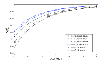
In this section, we use MATLAB based simulations to validate the accuracy of the analytical results and the tightness of the proposed performance bounds. Each point shown in the figures is the average result obtained from 100,000 simulations. The 95% confidence interval is also shown in each figure. For clarity, the simulation parameters adopted in this section are summarized in Table I.

Table I: SIMULATION PARAMETERS
Rateless Codes encoding parameters
Number of source packets kπ‘˜k 20,40204020,40
Number of internediate packets n𝑛n 212121, 414141
Parameter for bernoulli random variables Ξ·πœ‚\eta 0.30.30.3, 0.70.70.7
Pre-code π’žπ’ž\mathcal{C} (n,k,Ξ·)π‘›π‘˜πœ‚(n,k,\eta) LDPC codes
LT codes degree distribution
Standard degree distribution Ξ©3​G​P​P​(x)superscriptΞ©3𝐺𝑃𝑃π‘₯\Omega^{3GPP}(x)[6, Annex B]
Binomial degree distribution Ξ©d=()dn(2nβˆ’1),1≀d≀n\Omega_{d}=\frac{\left({}_{d}^{n}\right)}{(2^{n}-1)},1\leq d\leq n
Ideal soliton degree distribution Ξ©d=1d​(dβˆ’1),2≀d≀nformulae-sequencesubscriptΩ𝑑1𝑑𝑑12𝑑𝑛\Omega_{d}=\frac{1}{d(d-1)},2\leq d\leq n
and Ξ©1=1nsubscriptΞ©11𝑛\Omega_{1}=\frac{1}{n}
Robust soliton degree distribution c=0.04𝑐0.04c=0.04, Ξ΄=0.01𝛿0.01\delta=0.01

IV-A Verification of the Derived Bounds

In this sub-section, the number of source packets is set to be k=20π‘˜20k=20, and the degree distribution of Raptor codes follows the widely used ideal soliton degree distribution [4]. Besides, the pre-code π’žπ’ž\mathcal{C} is assumed to be (21,20,0.3)21200.3\left(21,20,0.3\right) and (21,20,0.7)21200.7\left(21,20,0.7\right) LDPC codes.

Refer to caption
Figure 2: The probabilities of successfully decoding all 20 source packets by the MU as a function of overhead γ𝛾\gamma of transmission by the BS

In Figs. 2, our analytical and simulation results are presented in terms of the probability Pr⁑[Amk]Prsuperscriptsubscriptπ΄π‘šπ‘˜\Pr\left[A_{m}^{k}\right] that the MU successfully decode all k=20π‘˜20k=20 source packets as a function of overhead Ξ³=m/kπ›Ύπ‘šπ‘˜\gamma=m/k of transmission by the BSs. As shown in Fig. 2, our analytical results, i.e., the upper and lower bound match the simulation results very well, which validates the accuracy of the analysis in this paper. However, when overhead γ𝛾\gamma is small, there is still a gap between the upper (lower) bounds and simulation results in Fig. 2. The gap between the exact value and the upper (lower) bound is caused by the approximation used in equation (3), and the gap between the exact value and the lower bound is caused by equation (2).

IV-B Investigation of the Impact of Degree Distribution on the Decoding Success Probability

When we fix the Pre-code π’žπ’ž\mathcal{C} as (21,20,0.7)21200.7\left(21,20,0.7\right), the degree distributionS of Raptor codes are chosen as the widely used ideal soliton degree distribution, the robust soliton degree distribution [4], the standardized degree distribution in 3GPP [6, Annex B]:

Ξ©3​G​P​P​(x)superscriptΞ©3𝐺𝑃𝑃π‘₯\displaystyle\Omega^{3GPP}(x) =\displaystyle= 0.0099​x+0.4663​x20.0099π‘₯0.4663superscriptπ‘₯2\displaystyle 0.0099x+0.4663x^{2}
+0.2144​x3+0.1152​x40.2144superscriptπ‘₯30.1152superscriptπ‘₯4\displaystyle+0.2144x^{3}+0.1152x^{4}
+0.1131​x10+0.0811​x110.1131superscriptπ‘₯100.0811superscriptπ‘₯11\displaystyle+0.1131x^{10}+0.0811x^{11}

and a Binomial degree distribution proposed in this paper (see Table I). As shown in Fig. 3(a) and 3(b), for different degree distributions, our analytical bounds are also corroborated by simulation results. Moreover, the performance of Raptor codes with the binomial degree distribution outperforms those with other three degree distributions. Additionally, the expression of decoding success probability of Raptor code with binomial degree distribution in Corollaries 5 and 4 has their computation superiority compared with the expression in Theorems 2 and 3. Therefore, we will focus on Raptor codes with the binomial degree distribution in the following simulations.
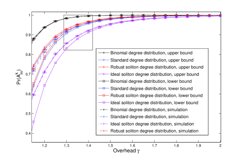
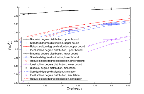
Refer to caption
(a) Full Scale
Refer to caption
(b) Zoom of the rectangular box in (a)
Figure 3: The probabilities of successfully decoding all 20 source packets by the MU as a function of overhead γ𝛾\gamma of transmission by the BS

IV-C Investigation of the Impact of kπ‘˜k on the Decoding Success Probability

When the number of source packets kπ‘˜k increases from 20 to 40, our analytical results still tightly match the simulation ones. As can be seen from Fig. 4(a) and 4(b), comparing transmitting 20 source packets with transmitting 40 ones, the BS can reduce the overhead Ξ³=m/kπ›Ύπ‘šπ‘˜\gamma=m/k of transmission that required to achieve the same performance, which leads to reduced transmission latency and energy consumption.
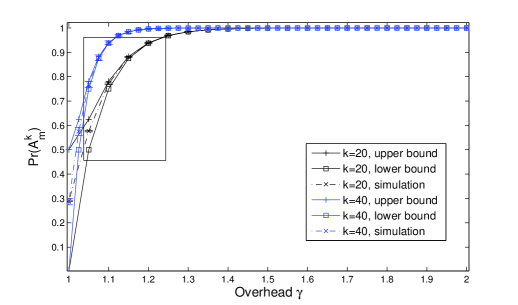
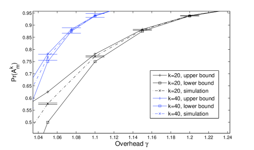
Refer to caption
(a) Full Scale
Refer to caption
(b) Zoom of the rectangular box in (a)
Figure 4: The probabilities of successfully decoding all 20 and 40 source packets by the MU as a function of overhead γ𝛾\gamma of transmission by the BS

IV-D Comparison of the Successful Transmission Probability for Raptor codes and Ideal Fountain codes

In Fig. 5(a) and 5(b), we compare the Raptor code to an ideal fountain code together with the baseline transmission without coding. As can be observed from 5(a) and 5(b), the performance gap between the Raptor code and the ideal fountain code is non-negligible because in the ideal fountain code the number of received symbols needed to decode the source symbols is exactly the number of source symbols, no matter which symbols are received. Hence, the decoding success probability of an ideal fountain code is as high as Pr⁑(Amk)=1,mβ‰₯kformulae-sequencePrsuperscriptsubscriptπ΄π‘šπ‘˜1π‘šπ‘˜\Pr\left(A_{m}^{k}\right)=1,m\geq k. Besides, the coding gain of Raptor codes compared with the baseline transmission without coding is shown to be tremendous. We apply Raptor codes and an ideal fountain code into a single BEC channel with different erasure probability p𝑝p. The probability that the receiver can decode all kπ‘˜k source packets based on the successfully received coded packets, denoted as Ps​u​csubscript𝑃𝑠𝑒𝑐P_{suc}, can be expressed as:

Ps​u​c​(T)subscript𝑃𝑠𝑒𝑐𝑇\displaystyle P_{suc}(T) =\displaystyle= βˆ‘m=kT(mT)Pr(Amk)pTβˆ’m(1βˆ’p)m\displaystyle\sum_{m=k}^{T}(_{m}^{T})\Pr\left(A_{m}^{k}\right)p^{T-m}(1-p)^{m}

As demonstrated in Fig. 5(a) and 5(b), for different erasure probability p𝑝p, transmission without coding can significantly reduce the overhead Ξ³=m/kπ›Ύπ‘šπ‘˜\gamma=m/k of transmitting that required to achieve the same performance. When the target performance, e.g., the probability of successful delivery is set to 0.95 for p=0.1𝑝0.1p=0.1, the ratio of the number of packets transmitted without using coding to that using Raptor code equals 2.069; for p=0.3𝑝0.3p=0.3, the ratio increases to 2.564. It seems that the ratio increases as the channel condition become worse. As for the comparison between the ideal fountain code and Raptor code, for the same target performance of0.95, for p=0.1𝑝0.1p=0.1, the ratio of the number of packets transmitted with Raptor code to that using ideal fountain code equals 1.16; for p=0.3𝑝0.3p=0.3, the ratio decreases to 1.11. It seems that the performance of Raptor code converges to that of the ideal fountain code when the channel condition become worse.
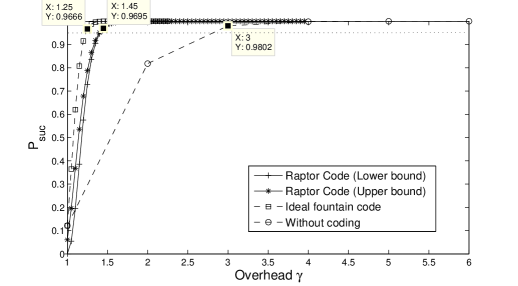
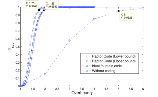
Refer to caption
(a) p=0.1
Refer to caption
(b) p=0.3
Figure 5: The probabilities of successfully decoding all 20 source packets by the MU as a function of overhead γ𝛾\gamma of transmission by the BS

V Conclusion

In this paper we focus on finite-length Raptor codes and derive upper and lower bounds on packet error performance of Raptor codes under maximum-likelihood (ML) decoding, which is measured by the probability that all source packets can be successfully decoded by a receiver with a given number of successfully received coded packets. ML decoding ensures successful decoding when a full-rank matrix is received. Due to the concatenated coding structure of Raptor codes, we have analyzed the rank behavior of product of two random matrix.

On the basis of the results presented in the paper, in the future, we plan to explore the optimum degree distribution and optimal parameter of Raptor codes in different channels.

Appendix A: Proof of Lemma 1

The event that (𝐆L​T;𝐇(nβˆ’k)Γ—n)(m+nβˆ’k)Γ—nsubscriptsuperscript𝐆𝐿𝑇subscriptπ‡π‘›π‘˜π‘›π‘šπ‘›π‘˜π‘›(\mathbf{G}^{LT};\mathbf{H}_{(n-k)\times n})_{(m+n-k)\times n} is a full rank matrix, i.e. its rank equals n𝑛n, is equivalent to the event that (𝐆L​T​𝐆p​r​e)mΓ—ksubscriptsuperscript𝐆𝐿𝑇superscriptπ†π‘π‘Ÿπ‘’π‘šπ‘˜(\mathbf{G}^{LT}\mathbf{G}^{pre})_{m\times k} is a full rank matrix.

Firstly we prove that the event that (𝐆L​T​𝐆p​r​e)mΓ—ksubscriptsuperscript𝐆𝐿𝑇superscriptπ†π‘π‘Ÿπ‘’π‘šπ‘˜(\mathbf{G}^{LT}\mathbf{G}^{pre})_{m\times k} is a full rank matrix is a sufficient condition for the event that (𝐆L​T;𝐇(nβˆ’k)Γ—n)(m+nβˆ’k)Γ—nsubscriptsuperscript𝐆𝐿𝑇subscriptπ‡π‘›π‘˜π‘›π‘šπ‘›π‘˜π‘›(\mathbf{G}^{LT};\mathbf{H}_{(n-k)\times n})_{(m+n-k)\times n} is a full rank matrix. Recall that 𝐇(nβˆ’k)Γ—n=[𝐏(nβˆ’k)Γ—k|𝐈(nβˆ’k)](nβˆ’k)Γ—nsubscriptπ‡π‘›π‘˜π‘›subscriptdelimited-[]conditionalsubscriptππ‘›π‘˜π‘˜subscriptπˆπ‘›π‘˜π‘›π‘˜π‘›\mathbf{H}_{(n-k)\times n}=[\mathbf{P}_{(n-k)\times k}|\mathbf{I}_{(n-k)}]_{(n-k)\times n} , 𝐆nΓ—kp​r​e=[𝐈k|𝐏kΓ—(nβˆ’k)]Tsuperscriptsubscriptπ†π‘›π‘˜π‘π‘Ÿπ‘’superscriptdelimited-[]conditionalsubscriptπˆπ‘˜subscriptππ‘˜π‘›π‘˜π‘‡\mathbf{G}_{n\times k}^{pre}=[\mathbf{I}_{k}|\mathbf{P}_{k\times(n-k)}]^{T} and 𝐇(nβˆ’k)Γ—n×𝐆nΓ—kp​r​e=𝟎subscriptπ‡π‘›π‘˜π‘›superscriptsubscriptπ†π‘›π‘˜π‘π‘Ÿπ‘’0\mathbf{H}_{(n-k)\times n}\times\mathbf{G}_{n\times k}^{pre}=\mathbf{0}. If (𝐆L​T;𝐇(nβˆ’k)Γ—n)superscript𝐆𝐿𝑇subscriptπ‡π‘›π‘˜π‘›(\mathbf{G}^{LT};\mathbf{H}_{(n-k)\times n}) is a full rank matrix, we can obtain that (𝐆L​T;𝐇(nβˆ’k)Γ—n)×𝐆p​r​e=(𝐆L​T​𝐆p​r​e;𝟎(nβˆ’k)Γ—k)superscript𝐆𝐿𝑇subscriptπ‡π‘›π‘˜π‘›superscriptπ†π‘π‘Ÿπ‘’superscript𝐆𝐿𝑇superscriptπ†π‘π‘Ÿπ‘’subscript0π‘›π‘˜π‘˜(\mathbf{G}^{LT};\mathbf{H}_{(n-k)\times n})\times\mathbf{G}^{pre}=(\mathbf{G}^{LT}\mathbf{G}^{pre};\mathbf{0}_{(n-k)\times k})is of full rank, i.e., (𝐆L​T​𝐆p​r​e)mΓ—ksubscriptsuperscript𝐆𝐿𝑇superscriptπ†π‘π‘Ÿπ‘’π‘šπ‘˜(\mathbf{G}^{LT}\mathbf{G}^{pre})_{m\times k} is a full rank matrix.

(𝐆mΓ—nL​T𝐇(nβˆ’k)Γ—n)​(𝐆p​r​e​𝐬T)superscriptsubscriptπ†π‘šπ‘›πΏπ‘‡subscriptπ‡π‘›π‘˜π‘›superscriptπ†π‘π‘Ÿπ‘’superscript𝐬𝑇\displaystyle\left(\begin{array}[t]{c}\mathbf{G}_{m\times n}^{LT}\\ \mathbf{H}_{(n-k)\times n}\end{array}\right)\left(\mathbf{G}^{pre}\mathbf{s}^{T}\right) =\displaystyle= (𝐘mΓ—1𝟎(nβˆ’k)Γ—1)subscriptπ˜π‘š1subscript0π‘›π‘˜1\displaystyle\left(\begin{array}[t]{c}\mathbf{Y}_{m\times 1}\\ \mathbf{0}_{(n-k)\times 1}\end{array}\right)

Then we prove that the event that (𝐆L​T​𝐆p​r​e)mΓ—ksubscriptsuperscript𝐆𝐿𝑇superscriptπ†π‘π‘Ÿπ‘’π‘šπ‘˜(\mathbf{G}^{LT}\mathbf{G}^{pre})_{m\times k} is a full rank matrix is a necessary condition for the event that (𝐆L​T;𝐇(nβˆ’k)Γ—n)(m+nβˆ’k)Γ—nsubscriptsuperscript𝐆𝐿𝑇subscriptπ‡π‘›π‘˜π‘›π‘šπ‘›π‘˜π‘›(\mathbf{G}^{LT};\mathbf{H}_{(n-k)\times n})_{(m+n-k)\times n} is a full rank matrix. Since 𝐇(nβˆ’k)Γ—n×𝐆nΓ—kp​r​e=𝟎subscriptπ‡π‘›π‘˜π‘›superscriptsubscriptπ†π‘›π‘˜π‘π‘Ÿπ‘’0\mathbf{H}_{(n-k)\times n}\times\mathbf{G}_{n\times k}^{pre}=\mathbf{0}, we can observe that row vector space of 𝐇(nβˆ’k)Γ—nsubscriptπ‡π‘›π‘˜π‘›\mathbf{H}_{(n-k)\times n} span the left null space of 𝐆nΓ—kp​r​esuperscriptsubscriptπ†π‘›π‘˜π‘π‘Ÿπ‘’\mathbf{G}_{n\times k}^{pre}, i.e., R​(𝐇(nβˆ’k)Γ—nT)=N​((𝐆nΓ—kp​r​e)T)𝑅superscriptsubscriptπ‡π‘›π‘˜π‘›π‘‡π‘superscriptsuperscriptsubscriptπ†π‘›π‘˜π‘π‘Ÿπ‘’π‘‡R(\mathbf{H}_{(n-k)\times n}^{T})=N((\mathbf{G}_{n\times k}^{pre})^{T}).

(𝐆nΓ—kp​r​e​𝐇nΓ—(nβˆ’k)T)superscriptsubscriptπ†π‘›π‘˜π‘π‘Ÿπ‘’superscriptsubscriptπ‡π‘›π‘›π‘˜π‘‡\displaystyle\left(\begin{array}[t]{c}\mathbf{G}_{n\times k}^{pre}\end{array}\mathbf{H}_{n\times(n-k)}^{T}\right) =\displaystyle= (𝐈k𝐏kΓ—(nβˆ’k)𝐏(nβˆ’k)Γ—k𝐈(nβˆ’k))nΓ—nsubscriptsubscriptπˆπ‘˜subscriptππ‘˜π‘›π‘˜subscriptππ‘›π‘˜π‘˜subscriptπˆπ‘›π‘˜π‘›π‘›\displaystyle\left(\begin{array}[t]{cc}\mathbf{I}_{k}&\mathbf{P}_{k\times(n-k)}\\ \mathbf{P}_{(n-k)\times k}&\mathbf{I}_{(n-k)}\end{array}\right)_{n\times n}

As we can see that rank of (𝐆nΓ—kp​r​e​𝐇nΓ—(nβˆ’k)T)superscriptsubscriptπ†π‘›π‘˜π‘π‘Ÿπ‘’superscriptsubscriptπ‡π‘›π‘›π‘˜π‘‡\left(\begin{array}[t]{c}\mathbf{G}_{n\times k}^{pre}\end{array}\mathbf{H}_{n\times(n-k)}^{T}\right) is n𝑛n, the span of (𝐆nΓ—kp​r​e​𝐇nΓ—(nβˆ’k)T)superscriptsubscriptπ†π‘›π‘˜π‘π‘Ÿπ‘’superscriptsubscriptπ‡π‘›π‘›π‘˜π‘‡\left(\begin{array}[t]{c}\mathbf{G}_{n\times k}^{pre}\end{array}\mathbf{H}_{n\times(n-k)}^{T}\right) is β„€2nsuperscriptsubscriptβ„€2𝑛\mathbb{Z}_{2}^{n}. Hence we can obtain that basis{N((𝐆nΓ—kp​r​e)T)}=basis{R(𝐇(nβˆ’k)Γ—nT)}=basis{β„€2n}\basis\{N((\mathbf{G}_{n\times k}^{pre})^{T})\}=basis\{R(\mathbf{H}_{(n-k)\times n}^{T})\}=basis\{\mathbb{Z}_{2}^{n}\}\backslash b​a​s​i​s​{R​(𝐆nΓ—kp​r​e)}π‘π‘Žπ‘ π‘–π‘ π‘…superscriptsubscriptπ†π‘›π‘˜π‘π‘Ÿπ‘’basis\{R(\begin{array}[t]{c}\mathbf{G}_{n\times k}^{pre}\end{array})\}, i.e., b​a​s​i​s​{R​(𝐆nΓ—kp​r​e)}βˆͺb​a​s​i​s​{N​((𝐆nΓ—kp​r​e)T)}=b​a​s​i​s​{β„€2n}π‘π‘Žπ‘ π‘–π‘ π‘…superscriptsubscriptπ†π‘›π‘˜π‘π‘Ÿπ‘’π‘π‘Žπ‘ π‘–π‘ π‘superscriptsuperscriptsubscriptπ†π‘›π‘˜π‘π‘Ÿπ‘’π‘‡π‘π‘Žπ‘ π‘–π‘ superscriptsubscriptβ„€2𝑛basis\{R(\begin{array}[t]{c}\mathbf{G}_{n\times k}^{pre}\end{array})\}\cup basis\{N((\mathbf{G}_{n\times k}^{pre})^{T})\}=basis\{\mathbb{Z}_{2}^{n}\}. By using the same idea, we can obtain that b​a​s​i​s​{R​((𝐆nΓ—kp​r​e)T)}βˆͺb​a​s​i​s​{N​(𝐆nΓ—kp​r​e)}=b​a​s​i​s​{β„€2n}π‘π‘Žπ‘ π‘–π‘ π‘…superscriptsuperscriptsubscriptπ†π‘›π‘˜π‘π‘Ÿπ‘’π‘‡π‘π‘Žπ‘ π‘–π‘ π‘superscriptsubscriptπ†π‘›π‘˜π‘π‘Ÿπ‘’π‘π‘Žπ‘ π‘–π‘ superscriptsubscriptβ„€2𝑛basis\{R((\mathbf{G}_{n\times k}^{pre})^{T})\}\cup basis\{N(\mathbf{G}_{n\times k}^{pre})\}=basis\{\mathbb{Z}_{2}^{n}\}. Once in binary field, no matter the formation of matrix, we have b​a​s​i​s​{R​((𝐆)T)}βˆͺb​a​s​i​s​{N​(𝐆)}=b​a​s​i​s​{β„€2n}π‘π‘Žπ‘ π‘–π‘ π‘…superscriptπ†π‘‡π‘π‘Žπ‘ π‘–π‘ π‘π†π‘π‘Žπ‘ π‘–π‘ superscriptsubscriptβ„€2𝑛basis\{R((\mathbf{G})^{T})\}\cup basis\{N(\mathbf{G})\}=basis\{\mathbb{Z}_{2}^{n}\}. For 𝐆mΓ—nL​Tsuperscriptsubscriptπ†π‘šπ‘›πΏπ‘‡\mathbf{G}_{m\times n}^{LT}, given that dim(N​(𝐆mΓ—nL​T)∩R​(𝐆nΓ—kp​r​e))=0dimension𝑁superscriptsubscriptπ†π‘šπ‘›πΏπ‘‡π‘…superscriptsubscriptπ†π‘›π‘˜π‘π‘Ÿπ‘’0\dim(N(\mathbf{G}_{m\times n}^{LT})\cap R(\mathbf{G}_{n\times k}^{pre}))=0, we can get

b​a​s​i​s​{N​(𝐆mΓ—nL​T)}π‘π‘Žπ‘ π‘–π‘ π‘superscriptsubscriptπ†π‘šπ‘›πΏπ‘‡\displaystyle basis\{N(\mathbf{G}_{m\times n}^{LT})\} =\displaystyle= b​a​s​i​s​{β„€2n}\b​a​s​i​s​{R​((𝐆mΓ—nL​T)T)}βŠ†b​a​s​i​s​{β„€2n}\b​a​s​i​s​{R​(𝐆nΓ—kp​r​e)}\π‘π‘Žπ‘ π‘–π‘ superscriptsubscriptβ„€2π‘›π‘π‘Žπ‘ π‘–π‘ π‘…superscriptsuperscriptsubscriptπ†π‘šπ‘›πΏπ‘‡π‘‡\π‘π‘Žπ‘ π‘–π‘ superscriptsubscriptβ„€2π‘›π‘π‘Žπ‘ π‘–π‘ π‘…superscriptsubscriptπ†π‘›π‘˜π‘π‘Ÿπ‘’\displaystyle basis\{\mathbb{Z}_{2}^{n}\}\backslash basis\{R((\mathbf{G}_{m\times n}^{LT})^{T})\}\subseteq basis\{\mathbb{Z}_{2}^{n}\}\backslash basis\{R(\mathbf{G}_{n\times k}^{pre})\}
⟹⟹\displaystyle\Longrightarrow b​a​s​i​s​{R​((𝐆mΓ—nL​T)T)}βŠ‡b​a​s​i​s​{R​(𝐆nΓ—kp​r​e)}π‘π‘Žπ‘ π‘–π‘ π‘…superscriptsubscriptπ†π‘›π‘˜π‘π‘Ÿπ‘’π‘π‘Žπ‘ π‘–π‘ π‘…superscriptsuperscriptsubscriptπ†π‘šπ‘›πΏπ‘‡π‘‡\displaystyle basis\{R((\mathbf{G}_{m\times n}^{LT})^{T})\}\supseteq basis\{R(\mathbf{G}_{n\times k}^{pre})\}

Because b​a​s​i​s​{R​(𝐇(nβˆ’k)Γ—nT)}=b​a​s​i​s​{β„€2n}\b​a​s​i​s​{R​(𝐆nΓ—kp​r​e)}π‘π‘Žπ‘ π‘–π‘ π‘…superscriptsubscriptπ‡π‘›π‘˜π‘›π‘‡\π‘π‘Žπ‘ π‘–π‘ superscriptsubscriptβ„€2π‘›π‘π‘Žπ‘ π‘–π‘ π‘…superscriptsubscriptπ†π‘›π‘˜π‘π‘Ÿπ‘’basis\{R(\mathbf{H}_{(n-k)\times n}^{T})\}=basis\{\mathbb{Z}_{2}^{n}\}\backslash basis\{R(\begin{array}[t]{c}\mathbf{G}_{n\times k}^{pre}\end{array})\}, b​a​s​i​s​{(𝐆L​T;𝐇(nβˆ’k)Γ—n)}=π‘π‘Žπ‘ π‘–π‘ superscript𝐆𝐿𝑇subscriptπ‡π‘›π‘˜π‘›absentbasis\{(\mathbf{G}^{LT};\mathbf{H}_{(n-k)\times n})\}=

b​a​s​i​s​{R​((𝐆mΓ—nL​T)T)}βˆͺb​a​s​i​s​{R​(𝐇(nβˆ’k)Γ—nT)}=b​a​s​i​s​{β„€2n}π‘π‘Žπ‘ π‘–π‘ π‘…superscriptsuperscriptsubscriptπ†π‘šπ‘›πΏπ‘‡π‘‡π‘π‘Žπ‘ π‘–π‘ π‘…superscriptsubscriptπ‡π‘›π‘˜π‘›π‘‡π‘π‘Žπ‘ π‘–π‘ superscriptsubscriptβ„€2𝑛\!\!\!\!\!\!basis\{R((\mathbf{G}_{m\times n}^{LT})^{T})\}\cup basis\{R(\mathbf{H}_{(n-k)\times n}^{T})\}=basis\{\mathbb{Z}_{2}^{n}\}. That is (𝐆L​T;𝐇(nβˆ’k)Γ—n)(m+nβˆ’k)Γ—nsubscriptsuperscript𝐆𝐿𝑇subscriptπ‡π‘›π‘˜π‘›π‘šπ‘›π‘˜π‘›(\mathbf{G}^{LT};\mathbf{H}_{(n-k)\times n})_{(m+n-k)\times n} is a full rank matrix, i.e. its rank equals n𝑛n.

Appendix B

The event that 𝐘=𝐆L​Tβ€‹π—π˜superscript𝐆𝐿𝑇𝐗\mathbf{Y}=\mathbf{G}^{LT}\mathbf{X}, where 𝐗=𝐆p​r​e​𝐬T𝐗superscriptπ†π‘π‘Ÿπ‘’superscript𝐬𝑇\mathbf{X}=\mathbf{G}^{pre}\mathbf{s}^{T} can be decoded by using ML decoding is equivalent to the event that (𝐆L​T​𝐆p​r​e)mΓ—ksubscriptsuperscript𝐆𝐿𝑇superscriptπ†π‘π‘Ÿπ‘’π‘šπ‘˜(\mathbf{G}^{LT}\mathbf{G}^{pre})_{m\times k} is a full rank matrix.

Firstly when using a BEC channel, a encoded bit is either correctly received or lost. We consider π˜β€²=𝐆′⁣L​T​𝐆p​r​e​𝐬Tsuperscriptπ˜β€²superscript𝐆′𝐿𝑇superscriptπ†π‘π‘Ÿπ‘’superscript𝐬𝑇\mathbf{Y}^{\prime}=\mathbf{G}^{\prime LT}\mathbf{G}^{pre}\mathbf{s}^{T} as the encoded bits generated by Raptor encoder. After transmission, the coded bits a receiver correctly received can be expressed as 𝐘=𝐆L​Tβ€‹π—π˜superscript𝐆𝐿𝑇𝐗\mathbf{Y}=\mathbf{G}^{LT}\mathbf{X}, where 𝐆L​Tsuperscript𝐆𝐿𝑇\mathbf{G}^{LT} is a part of 𝐆′⁣L​Tsuperscript𝐆′𝐿𝑇\mathbf{G}^{\prime LT}. Provided the rank of 𝐆L​Tsuperscript𝐆𝐿𝑇\mathbf{G}^{LT} is r, so the nullity of 𝐆L​Tsuperscript𝐆𝐿𝑇\mathbf{G}^{LT} is nβˆ’rπ‘›π‘Ÿn-r. Using ML decoding to decode 𝐗𝐗\mathbf{X} from 𝐘𝐘\mathbf{Y} is equivalent to solve the linear equation 𝐘=𝐆L​Tβ€‹π—π˜superscript𝐆𝐿𝑇𝐗\mathbf{Y}=\mathbf{G}^{LT}\mathbf{X} by using Gaussian Elimination method. The set of solutions to 𝐘=𝐆L​Tβ€‹π—π˜superscript𝐆𝐿𝑇𝐗\mathbf{Y}=\mathbf{G}^{LT}\mathbf{X} is an affine set. It has the form 𝐗=𝐗0+N(𝐆L​T)={𝐗0+x,x∈N(𝐆L​T)\mathbf{X}=\mathbf{X}_{0}+N(\mathbf{G}^{LT})=\{\mathbf{X}_{0}+x,x\in N(\mathbf{G}^{LT}) where 𝐗0=𝐆p​r​e​𝐬Tsubscript𝐗0superscriptπ†π‘π‘Ÿπ‘’superscript𝐬𝑇\mathbf{X}_{0}=\mathbf{G}^{pre}\mathbf{s}^{T} and 𝐗0∈R​(𝐆p​r​e)subscript𝐗0𝑅superscriptπ†π‘π‘Ÿπ‘’\mathbf{X}_{0}\in R(\mathbf{G}^{pre}). If we prove that the event that (𝐆L​T​𝐆p​r​e)mΓ—ksubscriptsuperscript𝐆𝐿𝑇superscriptπ†π‘π‘Ÿπ‘’π‘šπ‘˜(\mathbf{G}^{LT}\mathbf{G}^{pre})_{m\times k} is a full rank matrix is a sufficient condition for the event that (𝐆L​T;𝐇(nβˆ’k)Γ—n)(m+nβˆ’k)Γ—nsubscriptsuperscript𝐆𝐿𝑇subscriptπ‡π‘›π‘˜π‘›π‘šπ‘›π‘˜π‘›(\mathbf{G}^{LT};\mathbf{H}_{(n-k)\times n})_{(m+n-k)\times n} is a full rank matrix. Recall that 𝐇(nβˆ’k)Γ—n=[𝐏(nβˆ’k)Γ—k|𝐈(nβˆ’k)](nβˆ’k)Γ—nsubscriptπ‡π‘›π‘˜π‘›subscriptdelimited-[]conditionalsubscriptππ‘›π‘˜π‘˜subscriptπˆπ‘›π‘˜π‘›π‘˜π‘›\mathbf{H}_{(n-k)\times n}=[\mathbf{P}_{(n-k)\times k}|\mathbf{I}_{(n-k)}]_{(n-k)\times n} , 𝐆nΓ—kp​r​e=[𝐈k|𝐏kΓ—(nβˆ’k)]Tsuperscriptsubscriptπ†π‘›π‘˜π‘π‘Ÿπ‘’superscriptdelimited-[]conditionalsubscriptπˆπ‘˜subscriptππ‘˜π‘›π‘˜π‘‡\mathbf{G}_{n\times k}^{pre}=[\mathbf{I}_{k}|\mathbf{P}_{k\times(n-k)}]^{T} and 𝐇(nβˆ’k)Γ—n×𝐆nΓ—kp​r​e=𝟎subscriptπ‡π‘›π‘˜π‘›superscriptsubscriptπ†π‘›π‘˜π‘π‘Ÿπ‘’0\mathbf{H}_{(n-k)\times n}\times\mathbf{G}_{n\times k}^{pre}=\mathbf{0}. If dim{N​(𝐆mΓ—nL​T)∩R​(𝐆nΓ—kp​r​e)}=0dimension𝑁superscriptsubscriptπ†π‘šπ‘›πΏπ‘‡π‘…superscriptsubscriptπ†π‘›π‘˜π‘π‘Ÿπ‘’0\dim\{N(\mathbf{G}_{m\times n}^{LT})\cap R(\mathbf{G}_{n\times k}^{pre})\}=0, i.e., N​(𝐆mΓ—nL​T)∩R​(𝐆nΓ—kp​r​e)={Γ―ΒΏΕ“}𝑁superscriptsubscriptπ†π‘šπ‘›πΏπ‘‡π‘…superscriptsubscriptπ†π‘›π‘˜π‘π‘Ÿπ‘’Γ―ΒΏΕ“N(\mathbf{G}_{m\times n}^{LT})\cap R(\mathbf{G}_{n\times k}^{pre})=\{\textrm{\"{\i}\textquestiondown\oe}\} 𝐗0+N​(𝐆L​T)βˆ‰R​(𝐆nΓ—kp​r​e)subscript𝐗0𝑁superscript𝐆𝐿𝑇𝑅superscriptsubscriptπ†π‘›π‘˜π‘π‘Ÿπ‘’\mathbf{X}_{0}+N(\mathbf{G}^{LT})\notin R(\mathbf{G}_{n\times k}^{pre}). So 𝐗0+N​(𝐆L​T)subscript𝐗0𝑁superscript𝐆𝐿𝑇\mathbf{X}_{0}+N(\mathbf{G}^{LT}) is not the final solution when using ML decoding. 𝐗0=𝐙subscript𝐗0𝐙\mathbf{X}_{0}=\mathbf{Z} is the unique solution left. So the condition that the ML decoding can decode 𝐗𝐗\mathbf{X} correctly, i.e., 𝐗𝐗\mathbf{X} has the unique solution, is that dim{N​(𝐆mΓ—nL​T)∩R​(𝐆nΓ—kp​r​e)}=0dimension𝑁superscriptsubscriptπ†π‘šπ‘›πΏπ‘‡π‘…superscriptsubscriptπ†π‘›π‘˜π‘π‘Ÿπ‘’0\dim\{N(\mathbf{G}_{m\times n}^{LT})\cap R(\mathbf{G}_{n\times k}^{pre})\}=0, which is equivalent to the condition that (𝐆L​T​𝐆p​r​e)mΓ—ksubscriptsuperscript𝐆𝐿𝑇superscriptπ†π‘π‘Ÿπ‘’π‘šπ‘˜(\mathbf{G}^{LT}\mathbf{G}^{pre})_{m\times k} is a full rank matrix.

References

  • [1] A. Shokrollahi, "Raptor codes," IEEE Trans. Inf. Theory, vol. 52, no. 6, pp. 2551-2567, 2006.
  • [2] L. Feng, F. Chuan Heng, C. Jianfei, and C. Liang-Tien, "LT codes decoding: Design and analysis," in Proceedings of IEEE ISIT, 2009, pp. 2492-2496.
  • [3] H. D. T. Nguyen, T. Le-Nam, and H. Een-Kee, "On transmission efficiency for wireless broadcast using network coding and fountain codes," IEEE Commu Letters, vol. 15, no. 5, pp. 569-571, 2011.
  • [4] M. Luby, "LT codes," in Proceedings of the 43rd IEEE FOCS, 2002, pp. 271-280.
  • [5] N. Rahnavard, B. Vellambi, and F. Fekri, "Rateless codes with unequal error protection property," IEEE Trans. Inf. Theorys on, vol. 53, no. 4, pp. 1521-1532, April 2007.
  • [6] "3GPP TS 26.346 v6.1.0 (2005-06) Technical Specification Group Services and System Aspects; Multimedia Broadcast/Multicast Service; Protocols and Codecs," Tech. Rep.
  • [7] R. Karp, M. Luby, and A. Shokrollahi, "Finite length analysis of LT codes," in Proceedings of IEEE ISIT, 2004, p. 39.
  • [8] A. Shokrollahi, S. Lassen, and R. Karp, "Systems and processes for decoding chain reaction codes through inactivation," Feb. 15 2005, US Patent 6,856,263. [Online]. Available: http://www.google.com/patents/US6856263.
  • [9] P. Wang, G. Mao, Z. Lin, X. Ge, and B. Anderson, "Network coding based wireless broadcast with performance guarantee," IEEE Trans. Wireless Communications, vol.14, no.1, pp.532-544, Jan. 2015.
  • [10] T. Stockhammer, A. Shokrollahi, M. Watson, M. Luby, and T. Gasiba, "Application Layer Forward Error Correction for Mobile Multimedia Broadcasting," in Handbook of Mobile Broadcasting: DVB-H, DMB, ISDB-T and Media FLO, B. Furhet and S. Ahson, Eds. Boca Raton, FL: CRC Press, 2008, pp. 239-280..
  • [11] C. D. Meyer, Matrix analysis and applied linear algebra. SIAM, 2000.
  • [12] L. Comtet, Advanced Combinatorics. Reidel, 1974.