The use of a common location measure in the invariant coordinate selection and projection pursuit

Summary

Invariant coordinate selection (ICS) and projection pursuit (PP) are two methods that can be used to detect clustering directions in multivariate data by optimizing criteria sensitive to non-normality. In particular, ICS finds clustering directions using a relative eigen-decomposition of two scatter matrices with different levels of robustness; PP is a one-dimensional variant of ICS. Each of the two scatter matrices includes an implicit or explicit choice of location. However, when different measures of location are used, ICS and PP can behave counter-intuitively. In this paper we explore this behavior in a variety of examples and propose a simple and natural solution: use the same measure of location for both scatter matrices.

Keywords: Cluster analysis; Invariant coordinate selection; Projection pursuit; Robust scatter matrices; Location measures; Multivariate mixture model.

1 Introduction

Consider a multivariate dataset, given as an $n\times p$ data matrix $X$, and suppose we want to explore the existence of any clusters. One way to detect clusters is by projecting the data onto a lower dimensional subspace for which the data are maximally non-normal. Hence, methods that are sensitive to non-normality can be used to detect clusters.

One set of methods based on this principle is invariant coordinate selection (ICS), introduced by Tyler et al., (2009), together with a one-dimensional variant called projection pursuit (PP), introduced by Friedman and Tukey, (1974). ICS involves the use of two scatter matrices, $S_{1}=S_{1}(X)$ and $S_{2}=S_{2}(X)$ with $S_{2}$ chosen to be more robust than $S_{1}$. An eigen-decomposition of $S_{2}^{-1}S_{1}$ is carried out. If the data can be partitioned into two clusters, then typically the eigenvector corresponding to the smallest eigenvalue is a good estimate of the clustering direction. The main choice for the user when carrying out ICS is the choice of the two scatter matrices.

However, in numerical experiments based on a simple mixture of two bivariate normal distributions, some strange behaviour was noticed. In certain circumstances, ICS, and its variant PP, badly failed to pick out the right clustering direction. Eventually, it was discovered that the cause was the use of different location measures in the two scatter matrices. The purpose of this paper is to explore the reasons for this strange behaviour in detail and to demonstrate the benefits of using common location measures.

Section 2 gives some examples of scatter matrices and reviews the use of ICS and PP as clustering methods. Section 3 sets out the multivariate normal mixture model with two useful standardizations of the coordinate system. Section 4 demonstrates in the population setting an ideal situation where ICS and PP work as expected and where an analytic solution is available — the two-group normal mixture model where the two scatter matrices are given by the covariance matrix and a kurtosis-based matrix. Some examples with other robust estimators are given in Sections 5–6, which show how ICS and PP can go wrong when different location measures are used and how the problem is fixed by using a common location measure.

Notation. Univariate random variables, and their realizations, are denoted by lowercase letters, $x$, say. Multivariate random vectors, and their realizations, are denoted by lowercase bold letters, $\boldsymbol{x}$, say. A capital letter, $X$, say is used for $n\times p$ data matrix containing $p$ variables or measurements on $n$ observations; $X$ can be written in terms of its rows as

$$X=\begin{pmatrix}\boldsymbol{x}_{1}^{T}\\ \vdots\\ \boldsymbol{x}_{n}^{T}\end{pmatrix},$$

with $i$th row $\mathbf{\boldsymbol{x}}_{i}^{T}=(x_{i1},\ldots,x_{ip}),\ i=1,\ldots,n$.

2 Background

2.1 Scatter matrices

A scatter matrix $S(X)$, as a function of an $n\times p$ data matrix $X$ is a $p\times p$ affine equivariant positive definite matrix. Following Tyler et al., (2009), it is convenient to classify scatter matrices into three classes depending on their robustness.

• Class I: is the class of non-robust scatter matrices with zero breakdown point and unbounded influence function. Examples include the covariance matrix defined below in (1) and the kurtosis-based matrix in (2).

• Class II: is the class of scatter matrices that are locally robust, in the sense that they have bounded influence function and positive breakdown points not greater than $\frac{1}{p+1}$. An example from this class is the class of multivariate M-estimators, such as the M-estimate for the $t$-distribution (e.g., Kent et al.,, 1994; Arslan et al.,, 1995).

• Class III: is the class of scatter matrices with high breakdown points such as the Stahel-Donoho estimate, the minimum volume ellipsoid (mve) (Van Aelst and Rousseeuw,, 2009) and the constrained M-estimates, (e.g., Kent and Tyler,, 1996).

Each scatter matrix has an implicit location measure. Let us look at the main examples in more detail, and note what happens in $p=1$ dimension. The labels in parentheses are used as part of the notation later in the paper.

The sample covariance matrix (var) is defined by

$$S=\frac{1}{n}\sum_{i=1}^{n}(\boldsymbol{x}_{i}-\bar{\boldsymbol{x}})(\boldsymbol{x}_{i}-\bar{\boldsymbol{x}})^{T},$$ (1)

where for convenience here a divisor of $1/n$ is used, and where $\bar{\boldsymbol{x}}$ is the sample mean vector. The implicit measure of location is just the sample mean.

The kurtosis-based matrix (kmat) is defined by

$$K=\frac{1}{n}\sum_{i=1}^{n}\{(\boldsymbol{x}_{i}-\bar{\boldsymbol{x}})^{T}S^{-1}(\boldsymbol{x}_{i}-\bar{\boldsymbol{x}})\}(\boldsymbol{x}_{i}-\bar{\boldsymbol{x}})(\boldsymbol{x}_{i}-\bar{\boldsymbol{x}})^{T}.$$ (2)

Note that outlying observations are given higher weight than for the covariance matrix, so that $K$ is less robust than $S$. Again the implicit measure of location is just the sample mean. When $p=1$, the scatter matrix $S^{-1}K$ reduces to 3 plus the usual univariate kurtosis.

The $M$-estimator of scatter based on the multivariate $t_{\nu}$-distribution for fixed $\nu$ is the maximum likelihood estimate obtained by maximizing the likelihood jointly over scatter matrix $\Sigma$ and location vector $\mathbf{\boldsymbol{\mu}}$. If both parameters are unknown and $\nu\geq 1$, then under mild conditions on the data, the mle of $(\boldsymbol{\mu},\Sigma)$, is is the unique stationary point of the likelihood. Similarly, if $\nu\geq 0$ and $\mathbf{\boldsymbol{\mu}}$ is known, the mle of $\Sigma$, is is the unique stationary point of the likelihood (Kent et al.,, 1994). In either case, an iterative numerical algorithm is needed. Note that when $\mathbf{\boldsymbol{\mu}}$ is to be estimated as well as $\Sigma$, the mle of $\mu$ is the implicit measure of location for this scatter matrix. For this paper we limit attention to the choice $\nu=2$ (and label it below by t2).

The minimum volume ellipsoid (mve) estimate of scatter $S_{\text{mve}}$, introduced by Rousseeuw, (1985), is the ellipsoid that has the minimum volume among all ellipsoids containing at least half of observations, and its implicit estimate of location, $\bar{\boldsymbol{x}}_{\text{mve}}$, say, is the centre of that ellipsoid. Calculating the exact mve requires extensive computation. In practice, it is calculated approximately by considering only a subset of all subsamples that contain $50\%$ of the observations, (e.g., Van Aelst and Rousseeuw,, 2009; Maronna et al.,, 2006). If the location vector is specified, the search is limited to ellipsoids centred at this location measure.

When $p=1$, the mve reduces to the lshorth, defined as the length of the shortest interval that contains at least half of observations. The corresponding estimate of location, $\bar{\boldsymbol{x}}_{\text{lshorth}}$, say, is the midpoint of this interval. Calculating the lshorth around a known measure of location is trivial; just find the length of the interval that contains half of observations centered at this location measure. The lshorth was introduced by Grubel, (1988), building on earlier suggestion of Andrews et al., (1972) to use $\bar{\boldsymbol{x}}_{\text{lshorth}}$, which they called the shorth, as a location measure.

The minimum covariance determinant estimate of scatter (mcd), $S_{\text{mcd}}$ is defined as the covariance matrix of half of observations with the smallest determinant. The mcd location measure, $\bar{\boldsymbol{x}}_{\text{mcd}}$, say, is the sample mean of those observations. The mcd can be calculated approximately by considering only a subset of all subsamples that contain at least half of observations, (e.g., Rousseeuw and Driessen,, 1999). The mcd estimate of scatter with respect to a known location measure $\boldsymbol{\mu}$ is defined as the covariance matrix about $\boldsymbol{\mu}$ of half of observations with the smallest determinant. Recall that the covariance matrix about $\boldsymbol{\mu}$ for a dataset is given by $S+(\boldsymbol{\mu}-\bar{\boldsymbol{x}})(\boldsymbol{\mu}-\bar{\boldsymbol{x}})^{T}$, where $S$ and $\bar{\boldsymbol{x}}$ are the sample covariance matrix and mean vector of the dataset.

When $p=1$, the mcd reduces to a truncated variance, $v_{\text{trunc}}$, say, defined as the smallest variance of half the observations. Its implicit measure of location, $\bar{x}_{\text{trunc}}$, say, is the sample mean of that interval. Also, a modified definition of $v_{\text{trunc}}$ using a known location measure is trivial and does not require any search; just find the interval that contains half of observations centered at the given location measure and calculate the variance.

Routines are available in R (R Core Team,, 2014) to compute (at least approximately) these robust covariance matrices and their implicit location measures, in particular, tM from the package ICS (Nordhausen et al.,, 2008) for the multivariate $t$-distribution, cov.rob from the package MASS (Venables and Ripley,, 2002) for mve, and CovMcd from the package rrcov (Todorov and Filzmoser,, 2009) for mcd. Modified versions of these routines have been written by us to deal with the case of known location measures.

2.2 Invariant coordinate selection and projection pursuit

Given an $n\times p$ data matrix $X$, the ICS objective function is given by the ratio of quadratic forms

$$\kappa_{\text{ICS}}(\boldsymbol{a})=\frac{\boldsymbol{a}^{T}S_{1}\boldsymbol{a}}{\boldsymbol{a}^{T}S_{2}\boldsymbol{a}},\quad\boldsymbol{a}\in\mathbb{R}^{p},$$ (3)

where $S_{1}=S_{1}(X)$ and $S_{2}=S_{2}(X)$ are two scatter matrices. By convention, $S_{2}$ is chosen to be more robust than $S_{1}$. For exploratory statistical analysis, attention is focused on the choices for $\boldsymbol{a}$ maximizing or minimizing $\kappa_{\text{ICS}}(\boldsymbol{a})$. These values can be calculated analytically as the eigenvectors of $S_{2}^{-1}S_{1}$ corresponding to the maximum/minimum eigenvalues.

The original ICS method did not make a strong distinction between the largest and the smallest eigenvalues. However for clustering purposes between two groups, when the mixing proportion is not too far from $1/2$, it is the minimum eigenvalue which is of interest; see Section 4.

The method of PP can be regarded as a one-dimensional version of ICS. It looks for a linear projection $\boldsymbol{a}$ to maximize or minimize the criterion,

$$\kappa_{\text{PP}}(\boldsymbol{a})=\frac{s_{1}(X\boldsymbol{a})}{s_{2}(X\boldsymbol{a})}.$$ (4)

where $s_{1}=s_{1}(X\boldsymbol{a})$ and $s_{2}=s_{2}(X\boldsymbol{a})$ are two one-dimensional measures of spread. In general, optimizing $\kappa_{\text{PP}}(\boldsymbol{a})$ must be carried out numerically. Searching for a global optimum is computationally expensive, and the complexity of the search increases as the dimension $p$ increases. Alternatively, we can search for a local optimum starting from a sensible initial solution, such as the ICS optimum direction.

Both ICS and PP are equivariant under affine transformations. That is, if $X$ is transformed to $U=\boldsymbol{1}_{n}\boldsymbol{h}^{T}+XQ^{T}$, where $Q(p\times p)$ is nonsingular and $\boldsymbol{h}$ is a translation vector in $\mathbb{R}^{p}$, then for either ICS or PP the new optimal vector $\boldsymbol{b}$, say, for $U$ is related to the corresponding optimal vector $\boldsymbol{a}$ for $X$ by

$$\boldsymbol{b}\propto Q^{-T}\boldsymbol{a}.$$ (5)

For numerical work it is convenient to have an explicit notation for the different choices in ICS and PP. If Scat1 and Scat2 are the names of two types of multivariate scatter matrix, each computed with its own implicit location measure, then the corresponding versions of ICS and PP will be denoted

$$\text{ICS}:\text{Scat1}:\text{Scat2},\quad\text{and}\quad\text{PP}:\text{Scat1}:\text{Scat2}.$$

Note that PP is based on the univariate versions of Scat1 and Scat2. For example, ICS based on the covariance matrix and the minimum volume ellipsoid will be denoted by ICS:var:mve. Other choices for scatter matrices have been summarized in Section 2.

When a common location measure is imposed on Scat1 and Scat2, then this restriction will be indicated by the augmented notation

$$\text{ICS}:\text{Scat1}:\text{Scat2}:\text{Loc},$$

and similarly for PP. In this paper the only choice used for the location measure is the sample mean (mean). For example, ICS based on the covariance matrix and the minimum volume ellipsoid, both computed with respect to the mean vector, is denoted

$$\text{ICS}:\text{var}:\text{mve}:\text{mean}.$$

3 The two-group multivariate normal mixture model

The simple model used to demonstrate the main points of this paper is the two group multivariate normal mixture model, with density

$$f(\boldsymbol{x})=q\phi_{p}(\boldsymbol{x},\boldsymbol{\mu}_{1},\Omega)+(1-q)\phi_{p}(\boldsymbol{x},\boldsymbol{\mu_{2}},\Omega),$$

where $\phi_{p}$ is the multivariate normal density, $\boldsymbol{\mu}_{1}$ and $\boldsymbol{\mu}_{2}$ are two mean vectors, $\Omega$ is a common covariance matrix, and $0<q<1$ is the mixing proportion. Even in this simple case, major problems with ICS and PP can arise.

Since ICS and PP are affine equivariant, we may without loss of generality choose the coordinate system so that

$$\boldsymbol{\mu_{1}}=\alpha\boldsymbol{e_{1}},\quad\boldsymbol{\mu_{2}}=-\alpha\boldsymbol{e_{1}},\quad\Omega=I_{p},$$

where $\boldsymbol{e_{1}}=(1,0,\ldots,0)^{T}$ is a unit vector along the first coordinate axis, and $\alpha>0$. That is, $\boldsymbol{\mu_{1}}$ and $\boldsymbol{\mu_{2}}$ lie equally spaced about the origin along the first coordinate axis, and the covariance matrix of each component equals the identity matrix.

A random vector $\mathbf{\boldsymbol{x}}$ from the mixture model can also be given a stochastic representation,

$$\boldsymbol{x}=\alpha s\boldsymbol{e}_{1}+\boldsymbol{\epsilon},$$

where $\boldsymbol{\epsilon}\sim N_{p}(0,I_{p})$ independently of an indicator variable $s$,

$$s=\left\{\begin{array}[]{rl}1&\text{ with probability }q\\ -1&\text{ with probability }(1-q)\\ \end{array}\right..$$

Moments under the mixture model are calculated most simply in terms of this stochastic representation. In particular,

$$\boldsymbol{\mu}_{x}=E(\boldsymbol{x})=q\boldsymbol{\mu}_{1}+(1-q)\boldsymbol{\mu}_{2}=(2q-1)\alpha\boldsymbol{e}_{1},\quad E(\boldsymbol{xx}^{T})=\alpha^{2}\boldsymbol{e}_{1}\boldsymbol{e}_{1}^{T}+I_{p},$$

so that the covariance matrix is

$$\Sigma_{x}=\text{var}(\boldsymbol{x})=E(\boldsymbol{xx}^{T})-\boldsymbol{\mu}_{x}\boldsymbol{\mu}_{x}^{T}=4q(1-q)\alpha^{2}\boldsymbol{e}_{1}\boldsymbol{e}_{1}^{T}+I_{p}.$$ (6)

For practical work it is also convenient to consider a standardization for which the overall covariance matrix is the identity matrix. That is, define a new random vector

$$\boldsymbol{y}=C^{-1}\boldsymbol{x},$$ (7)

where $C^{-1}=\text{diag}(1/c_{1},\ldots,1/c_{p})$, where $c_{1}=\{1+4q(1-q)\alpha^{2}\}^{1/2}$, and $c_{2}=\cdots=c_{p}=1$. Then $\boldsymbol{y}$ has a stochastic representation

$$\boldsymbol{y}=\delta s\boldsymbol{e}_{1}+\boldsymbol{\eta},$$

where

$$\delta=\alpha/\{1+4q(1-q)\alpha^{2}\}^{1/2},$$ (8)

and

$$\boldsymbol{\eta}\sim N_{p}(0,\text{diag}(\sigma^{2}_{\eta},1,\ldots,1))$$

where the first diagonal term $\sigma^{2}_{\eta}$ has two equivalent formulas,

$$\sigma^{2}_{\eta}=\{1+4\alpha^{2}q(1-q)\}^{-1}\quad\text{or}\quad\sigma^{2}_{\eta}=1-4q(1-q)\delta^{2}$$

The first two moments of $\boldsymbol{y}$ are

$$\boldsymbol{\mu}_{y}=(2q-1)\delta\boldsymbol{e}_{1},\quad\Sigma_{y}=I_{p}.$$

4 A population example: PP based on the kurtosis and ICS based on the kurtosis-based matrix and the covariance matrix

In this section we look at ICS:kmat:var and PP:kmat:var in the population case. In this setting it is possible to derive analytic results. Note that since kmat is based on fourth moments it is less robust than the variance matrix; hence kmat is listed first.

Recall the kurtosis of a univariate random variable $u$, say, with mean $\mu_{u}$, is defined by

$$\text{kurt}(u)=\frac{\text{E}\{(u-\mu_{u})^{4}\}}{\left[\text{E}\{(u-\mu_{u})^{2}\}\right]^{2}}-3.$$

The univariate kurtosis is zero when the random variable has normal distribution. For non-normal distributions the kurtosis lies in the interval $[-2,\infty]$ and is often nonzero.

Peña and Prieto, (2001) studied the population version of PP:kmat:var and showed that when the mixing proportion is not too far from $1/2$ (more precisely, if $q(1-q)>1/6$, i.e. $0.21<q<0.79$), then minimizing the PP objective function picks out the correct clustering direction.

Their result can be derived simply as follows. Let $\mathbf{\boldsymbol{a}}\in\mathbb{R}^{p}$ be a unit vector. Write $\mathbf{\boldsymbol{a}}^{T}\mathbf{\boldsymbol{x}}=\alpha a_{1}s+v$, where $v=\mathbf{\boldsymbol{a}}^{T}\mathbf{\boldsymbol{\epsilon}}\sim N(0,1)$ is independent of $s$. The moments of $s$ are E$(s)=$E$(s^{3})=m$, say, where

$$m=2q-1,$$ (9)

and E$(s^{2})=$ E$(s^{4})=1$. Hence, var$(s)=\sigma^{2}$, say, where

$$\sigma^{2}=4q(1-q).$$ (10)

Then

$$\text{kurt}(s)=-6+4/\sigma^{2}.$$

It can be checked that $\text{kurt}(s)<0$ provided $q(1-q)>1/6$.

Next, we use the property that if $u_{1},u_{2}$ are independent random variables with the same variance, and if $\delta_{1},\delta_{2}$ are coefficients satisfying $\delta_{1}^{2}+\delta_{2}^{2}=1$, then

$$\text{kurt}(\delta_{1}u_{1}+\delta_{2}u_{2})=\delta_{1}^{4}\text{kurt}(u_{1})+\delta_{2}^{4}\text{kurt}(u_{2}).$$

Applying this result to $\mathbf{\boldsymbol{a}}^{T}\mathbf{\boldsymbol{x}}$ yields

$$\text{kurt}(\mathbf{\boldsymbol{a}}^{T}\mathbf{\boldsymbol{x}})=\frac{a_{1}^{4}\alpha^{4}\sigma^{4}}{(\alpha^{2}a_{1}^{2}\sigma^{2}+1)^{2}}\text{kurt}(s).$$ (11)

Provided $\text{kurt}(s)<0$, (11) is minimized when $a_{1}^{2}$ is maximized, that is, if $a_{1}^{2}=1$, so that $\mathbf{\boldsymbol{a}}=\pm e_{1}$ picks out the first coordinate axis.

The ICS calculations proceed similarly. First note that, the first diagonal term in $\Sigma_{x}$, defined in (6), can be expressed in terms of $\sigma^{2}$, defined in (10), as $\alpha^{2}\sigma^{2}+1$.

The first factor in the population version of $K$ defined in (2), $K_{x}$, say, is given by

$$(\boldsymbol{x}-\boldsymbol{\mu}_{x})^{T}\Sigma_{\boldsymbol{x}}^{-1}(\boldsymbol{x}-\boldsymbol{\mu}_{x})=\frac{(x_{1}-\alpha m)^{2}}{1+\alpha^{2}\sigma^{2}}+x_{2}^{2}+\cdots+x_{p}^{2}=D^{2},\text{ say,}$$

where $m$ is defined in (9). Note that $D^{2}$ is an even function in $x_{2},\ldots,x_{p}$. Hence by symmetry all the off-diagonal terms in $K_{x}$ vanish. The first diagonal term is given by

$$E\{D^{2}(x_{1}-\alpha m)^{2}\}=(1+\alpha^{2}\sigma^{2})(p+2)+\frac{\alpha^{4}\sigma^{4}\text{kurt}(s)}{(1+\alpha^{2}\sigma^{2})}.$$

The remaining diagonal terms, $j=2,\ldots,p$ are given by

$$E\{D^{2}x_{j}^{2}\}=p+2.$$

Hence $\Sigma_{x}^{-1}K_{x}$ reduces to

$$\text{diag}(p+2+\frac{\text{kurt}(s)\alpha^{4}\sigma^{4}}{(1+\alpha^{2}\sigma^{2})},p+2,\ldots,p+2).$$

These diagonal values are the eigenvalues. Hence provided $\text{kurt}(s)<0$, $\kappa_{\text{ICS}}$ is minimized when $\boldsymbol{a}=\boldsymbol{e}_{1}$, that is, when $\boldsymbol{a}$ picks out the clustering direction.

If $p=2$, we can write a unit vector as $\boldsymbol{a}=(\cos\theta,\sin\theta)^{T}$, and since $\mathbf{\boldsymbol{a}}$ and $-\boldsymbol{a}$ define the same axis, we can parameterize the ICS and PP objective functions in terms of $\theta,\ -\pi/2\leq\theta\leq\pi/2$. Plots of $\kappa_{\text{ICS}}(\theta)$ and $\kappa_{\text{PP}}(\theta)$ for $\alpha=3$ and $q=1/2$ are shown in Figure 1.

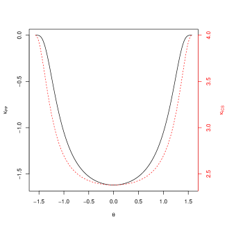
Figure 1: Plot of the population criteria $\kappa_{\text{ICS}}(\theta)$ (red dotted line), and $\kappa_{\text{PP}}(\theta)$ (solid black line) versus $\theta$, for $q=1/2$, $\alpha=3$.

For numerical work, especially when the underlying mixture model is unknown, the only feasible standardization is to ensure the overall variance matrix $\Sigma_{y}$ is the identity rather than the within group variance matrix. In terms of the population model of this section, it means working with $\mathbf{\boldsymbol{y}}$ from (7) rather than $\mathbf{\boldsymbol{x}}$. If $p=2$ and $\mathbf{\boldsymbol{b}}\propto(\cos\phi,\sin\phi)^{T}$, say, is also written in polar coordinates, then from (5) and (7) $\mathbf{\boldsymbol{a}}$ and $\mathbf{\boldsymbol{b}}$ are related by

$$\mathbf{\boldsymbol{b}}\propto C\mathbf{\boldsymbol{a}},$$

hence, $\phi$ and $\theta$ are related by

$$\begin{pmatrix}\cos\phi\\ \sin\phi\end{pmatrix}\propto\begin{pmatrix}c_{1}&0\\ 0&c_{2}\end{pmatrix}\begin{pmatrix}\cos\theta\\ \sin\theta\end{pmatrix}.$$

Thus,

$$\tan\phi=c\tan\theta,$$

where $c=c_{2}/c_{1}$.

The plot of the ICS and PP objective functions in Figure 2 shows that there is a sharper minimum in $\phi$ coordinates than in $\theta$ coordinates because under our mixture model $c$ is less than 1. If $\mathbf{\boldsymbol{x}}$ is scaled as in (7) with $c_{1}>c_{2}$, i.e $c>1$, then there will be a wider minimum in $\phi$.

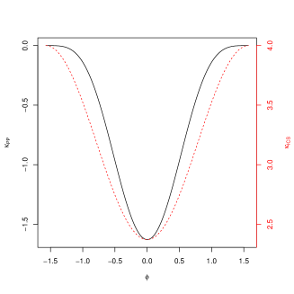
Figure 2: Plot of the population criteria $\kappa_{\text{ICS}}(\phi)$ (red dotted line), and $\kappa_{\text{PP}}(\phi)$ (solid black line) versus $\phi$, for $q=1/2$, and $\delta=0.95$.

5 The effect of using a common location measure on ICS and PP

As we mentioned earlier in Section 2.2, the ICS and PP criteria are expected to have similar behaviour to the kurtosis-based criteria in Section 4. Namely, they are expected to be minimized in the clustering direction when the mixing proportion is not too far from 1/2.

However, when applying ICS with at least one robust estimate of scatter (mainly from Class III), some peculiar behaviour was observed. In particular, the ICS criterion was often maximized in the clustering direction rather than minimized.

Here is an explanation. Under the two-group mixture model with one group slightly bigger than the other, a class III scatter matrix will typically home in on the larger group, with its corresponding location measure at the center of this group and its estimate of the scatter matrix capturing the spread of this group. The other scatter matrix (Class I or II) will measure the overall scatter of the data with its corresponding location measure at the overall center of the data. The result is erratic behaviour in $\kappa_{\text{ICS}}$ and $\kappa_{\text{PP}}$.

Imposing a common location measure on the two scatter matrices fixes this problem. Here is an example in $p=2$ dimensions to illustrate the issues in greater detail.

In this example we look at ICS:var:mve for the population bivariate normal mixture model in Section 3, with $q=1/2$ and any value of $\alpha>0$, i.e. $0\leq\delta\leq 1$, where $\delta$ is given in (8). Standardize the coordinate system so that the overall covariance matrix is the identity, $\Sigma_{y}=I_{2}$. Let $\Sigma_{\text{mve}}$ denote the population minimum volume ellipsoid scatter matrix.

Then it turns out that $\Sigma_{\text{mve}}$ is the within-group covariance matrix for (either) one of the groups,

$$\Sigma_{\text{mve}}=\begin{pmatrix}1-\delta^{2}&0\\ 0&1\end{pmatrix},$$ (12)

where $0\leq\delta\leq 1$ is given in (8). The implicit estimate of the center of the data will be given by the center of either group, $\pm\delta\boldsymbol{e}_{1}$; both values fit equally well.

Figure 3: Plot of the population criterion of ICS:var:mve vs. $\phi$ for $\delta=0.9$.

Figure 3 shows that the clustering direction estimated by the ICS:var:mve method is the direction that minimizes $\kappa_{\text{ICS}}$ (the eigenvector of the smallest eigenvalue of $\Sigma_{\text{mve}}^{-1}$), namely $(0,1)^{T}$, i.e. $\phi=\pm\pi/2$. However, the true direction of group separation direction is $(1,0)^{T}$, i.e. $\phi=0$.

Next consider ICS:var:mve:mean, i.e. the common mean version of the previous example. The overall mean of the data is at the origin. When $\Sigma_{\text{mve}}$ is constrained to have its location measure at the origin, then the ICS criterion now picks out the true clustering direction. In order to give an analytic proof of this result, we restrict attention to the the limiting case of the balanced mixture model, i.e when $\delta=1,\ q=1/2$. Hence, the group components will lie on two parallel vertical lines with means

$$\mu_{1}=(1,0)^{T},\ \ \mu_{2}=(-1,0)^{T},$$

and within-group covariance matrix

$$\begin{pmatrix}0&0\\ 0&1\end{pmatrix}.$$

In this setting, it can be shown that the population version of the MVE matrix, $\Sigma_{\text{mve}}$, say, takes the form

$$\Sigma_{\text{mve}}=c_{t}\Sigma_{t}=\begin{pmatrix}2&0\\ 0&2d^{2}\end{pmatrix},$$

where $d=\Phi^{-1}(.75)=0.674$, the 75th quantile of the standard normal distribution (see the Appendix). Hence the dominant eigenvector is $\mathbf{\boldsymbol{e}}_{1}$. The ellipse of $\Sigma_{\text{mve}}$ is plotted in Figure 4. Figure 5 shows that the criterion of ICS:var:mve:mean, $\kappa_{\text{ICS}:\mu}(\phi)$ picks out the correct clustering direction $\mathbf{\boldsymbol{e}}_{1}$.

Figure 4: Plot of the ellipse of the constrained $\Sigma_{\text{mve}}$.

Figure 5: Plot of the population criteria of ICS:var:mve:mean, $\kappa_{\text{ICS}:\mu}(\phi)$.

Like ICS, PP can fail to detect the clustering direction if applied using different location measures. The reason for that is the projection direction that separates the data into two groups with one slightly bigger than the other, the more robust measure of spread will be located at the larger group. In Section 6, we give a detailed numerical example of the problem arising from using two different location measures in PP:var:mcd, and how the problem is fixed by using a common location measure.

6 Examples

Overview

In this section, we give numerical examples that demonstrate different ways in which ICS and/or PP can go wrong. We also show the effect of using common location measures in these examples. We use one simulated data set and apply different ICS and PP methods, with and without imposing a common location measure (the mean).

A two-dimensional data set of size $n=500$ is generated from the balanced mixture model, defined in Section 3, with $q=1/2$, and $\alpha=3$, so that $\delta=0.95$. Thus the two groups are well-separated and no sensible statistical method should have any problem finding the two clusters. All calculations are done after standardization with respect to the “total” coordinates. That is, the data matrix $Y(500\times 2)$ is standardized to have sample mean $\mathbf{\boldsymbol{0}}$ and sample covariance matrix $I_{2}$.

The ICS and PP methods used are:

• (PP,ICS):var:t2 with corresponding criteria $\kappa_{\text{ICS}}^{1}$, and $\kappa_{\text{ICS}}^{1}$.

• (PP,ICS):var:mcd with corresponding criteria $\kappa_{\text{ICS}}^{2}$, and $\kappa_{\text{PP}}^{2}$.

• (PP,ICS):var:mve with corresponding criteria $\kappa_{\text{ICS}}^{3}$, and $\kappa_{\text{PP}}^{3}$.

• (PP,ICS):t2:mcd with corresponding criteria $\kappa_{\text{ICS}}^{4}$, and $\kappa_{\text{PP}}^{4}$.

• (PP,ICS):t2:mve with corresponding criteria $\kappa_{\text{ICS}}^{5}$, and $\kappa_{\text{PP}}^{5}$.

When imposing the mean as the common location measure, the ICS and PP criteria will be denoted by $\kappa_{\text{ICS:mean}}^{j}$ and $\kappa_{\text{PP:mean}}^{j}$, where $j=1,\ldots,5$.

To understand the behaviour of the ICS and PP, their criteria are plotted against $-\pi/2\leq\phi\leq\pi/2$. The plots are shown in Figure 6.

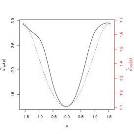
(a) (PP,ICS):var:t2

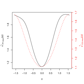
(b) (PP,ICS):var:t2:var

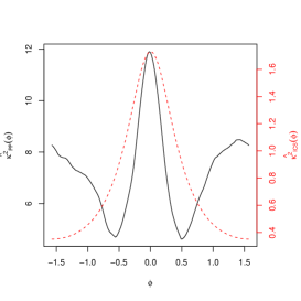
(c) (PP,ICS):var:mcd

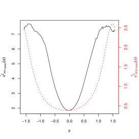
(d) (PP,ICS):var:mcd:mean

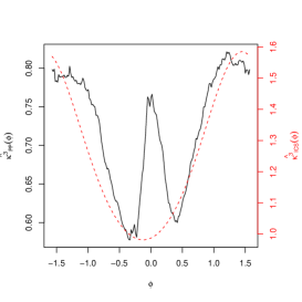
(e) (PP,ICS):var:mve

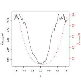
(f) (PP,ICS):var:mve:mean

Figure 6:

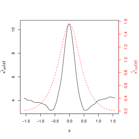
(g) (PP,ICS):t2:mcd

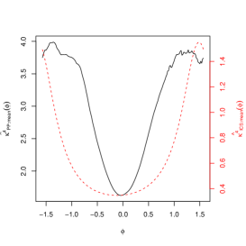
(h) (PP,ICS):t2:mcd:mean

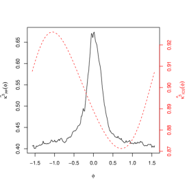
(i) (PP,ICS):t2:mve

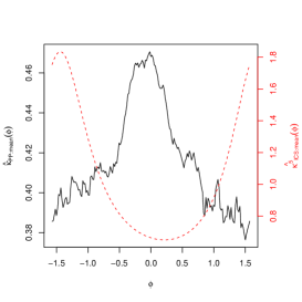
(j) (PP,ICS):t2:mve:mean

Figure 6: For $\delta=0.95$ and $q=1/2$, plots of different ICS (red dashed curve) and PP (black solid curve) criteria without (left) and with imposing a common location measure (right).

From the panels in Figure 6, we make the following remarks based on the simulated data set:

• Panel (a) shows that ICS:var:t2 and PP:var:t2 work well since $\bar{\mathbf{\boldsymbol{y}}}$ and $\bar{\mathbf{\boldsymbol{y}}_{t2}}$ are approximately equal. Hence, imposing a common location measure has little effect, as shown in (b).

• Panels (c), (e), (g), (i) show examples when ICS and/or PP go wrong because of the difference in the location measures.

• Using a common location measure fixes the problem in panel (d) for (PP, ICS):var:mcd, panel (f) for (PP, ICS):var:mve, and panel(h) for (PP, ICS):t2:mcd.

• From panel (j), using a common location measure in PP:t2:mve:mean does not seem to work well. The reason might be due to the unstable behaviour of the mve and lshorth.

• The plots generally suggest that PP will be more accurate than ICS, since the PP plots are narrower at the clustering direction than the ICS plot. This property has been confirmed empirically in Alashwali, (2013) for certain multivariate normal mixture models and choices of scatter matrix.

• Similar patterns are seen with most simulated data sets from this model.

Behaviour of ICS:var:mcd

To gain a deeper understanding of the behaviour of ICS:var:mcd in panel 6 (c) and the effect of forcing a common location measure on mcd in panel (d), we plot the ellipses of $S_{\text{mcd}}$ ( with and without imposing a common location meaure) and superimpose it on the data points of our example. The plots are shown in panels 7 (a) and (b). The behaviour in this example agrees with the interpretation given for the population example in Section 5.

(a)

(b)

Figure 7: Plots of the ellipses of mcd scatter matrix based on (a) mcd location measure, and (b) the sample mean, superimposed on data of size $n=500$, distributed as mixtures of two normal distributions.

Behaviour of PP:var:mcd

The objective function for PP:var:mcd, has a similar problem to ICS; it is maximized rather than minimized near the correct clustering direction.

To understand this behaviour in more detail, we plot in Figure 8 one-dimensional histograms after projections by the following choices for the angle $\phi$: $0^{\circ}$, $15^{\circ}$, $30^{\circ}$, and $90^{\circ}$. For each histogram, we plot the $50\%$ of the data that has the smallest variance, and the corresponding location measure $\bar{x}_{\text{trunc}}$. The plots are repeated where the location measure is constrained at the sample mean $\bar{x}=0$.

(a) $v_{\text{trunc}}=0.08$, $\bar{x}_{\text{trunc}}=-0.93$

(b) $v_{\text{trunc}}=0.54$, $\bar{x}=0$

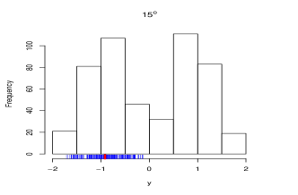
(c) $v_{\text{trunc}}=0.14$, $\bar{x}_{\text{trunc}}=-0.92$

(d) $v_{\text{trunc}}=0.42$, $\bar{x}=0$

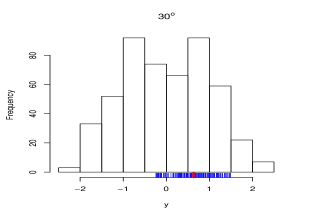
(e) $v_{\text{trunc}}=0.21$, $\bar{x}_{\text{trunc}}=0.63$

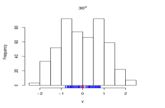
(f) $v_{\text{trunc}}=0.26$, $\bar{x}_{\text{trunc}}=0.02$

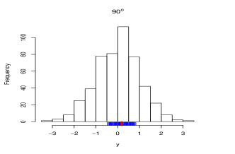
(g) $v_{\text{trunc}}=0.12$, $\bar{x}_{\text{trunc}}=0.18$

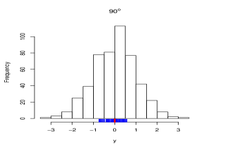
(h) $v_{\text{trunc}}=0.14$, $\bar{x}_{\text{trunc}}=0$

Figure 8: Histograms of $0^{\circ},15^{\circ},30^{\circ}$ and $90^{\circ}$ projections. Left panels show the vectors of $50\%$ of data with the smallest variance (the blue lines), and its location measure (the red lines), right panels show the $50\%$ of data with the smallest variance computed around the mean 0.

The shape of the histograms depends on of the projection directions. Note that as $v_{\text{trunc}}$ gets smaller, the PP criterion $\kappa_{\text{PP}}$ gets larger.

• The $0^{\circ}$ projection produces two widely separated groups with one group is slightly bigger than the other. In this case, $\bar{x}_{\text{trunc}}$ is at the larger group and $v_{\text{trunc}}$ is essentially the variance of this group. Hence $v_{\text{trunc}}$ takes its smallest value and $\kappa_{\text{PP}}$ is largest.

• The $15^{\circ}$ projection produces two slightly separated groups with within-group variance is larger than in the $0^{\circ}$ projection. The value of $v_{\text{trunc}}$ is larger than for $0^{\circ}$.

• The $30^{\circ}$ projection produces one group, with a pseudo-uniform distribution. The value of $v_{\text{trunc}}$ is larger than for $15^{\circ}$.

• The $90^{\circ}$ projection produces one normally distributed group. The value for $v_{\text{trunc}}$ becomes small again.

Constraining the mean to be at the origin fixes the problem. The value of $v_{\text{trunc}}$ steadily decreases from $0^{\circ}$ to $90^{\circ}$.

Appendix

Consider the limiting balanced bivariate normal mixture model,

$$\mathbf{\boldsymbol{y}}=s\mathbf{\boldsymbol{e}}_{1}+z\mathbf{\boldsymbol{e}}_{2},$$

where $s=\pm 1$, each with probability 1/2, independent of $z\sim N(0,1)$, and $\mathbf{\boldsymbol{e}}_{1}=(1,0)^{T}$, $\mathbf{\boldsymbol{e}}_{2}=(0,1)^{T}$. This model is standardized with respect to the “total” coordinates; i.e. $E(\mathbf{\boldsymbol{y}})=\mathbf{\boldsymbol{0}}$ and $\text{var}(\mathbf{\boldsymbol{y}})=I_{2}$. The model can also be described in terms of a mixture of two normal distributions, concentrated on the vertical lines $y_{1}=1$ and $y_{1}=-1$.

In this appendix we shall show that the population version of the mve, constrained to be centred at at the origin, is given by

$$\Sigma_{\text{mve}}=\begin{bmatrix}2&0\\ 0&d^{2}\end{bmatrix},$$

where $d=\Phi^{-1}(.75)$ in terms of the cumulative distribution function of the $N(0,1)$ distribution.

First let $u_{1}<u_{2}$ be two possible values for $y_{2}$ and consider and ellipse based on a matrix $\Sigma$, with inverse $\Sigma^{-1}=\Omega$,

$$\mathbf{\boldsymbol{y}}^{T}\Omega\mathbf{\boldsymbol{y}}=1$$ (A.1)

which intersects the vertical lines at these points,

$$\begin{bmatrix}1&u_{1}\end{bmatrix}\Omega\begin{bmatrix}1\\ u_{1}\end{bmatrix}=1,\quad\begin{bmatrix}1&u_{2}\end{bmatrix}\Omega\begin{bmatrix}1\\ u_{2}\end{bmatrix}=1.$$ (A.2)

By symmetry the ellipse also intersects the points $(-1,-u_{1})^{T}$ and $(-1,-u_{2})^{T}$. Note that $\Sigma$ will be a candidate for the mve matrix if the interior of the ellipse covers 50% of the probability mass, that is,

$$\Phi(u_{2})=\Phi(u_{1})+1/2.$$ (A.3)

If $u_{1}$ and $u_{2}$ are finite, then necessarily $u_{1}<0$ and $u_{2}>0$.

The proof will proceed in two stages. First, for fixed $u_{1},\ u_{2}$ satisfying (A.3), we choose $\Sigma$ to minimize $\det(\Sigma)$ (or equivalently maximize $\det(\Omega)$). Secondly, we optimize over the choice of $u_{1},\ u_{2}$.

Thus, start with a fixed pair of values $u_{1},\ u_{2}$ satisfying (A.3). If $\mathbf{\boldsymbol{y}}=(1,u)^{T}$ represents a point on one of the vertical lines, then the intersection with the ellipse (A.1) can be written

$$\omega_{11}+2\omega_{12}u+\omega_{22}u^{2}=1,$$

or equivalently as the quadratic equation in u,

$$Au^{2}+Bu+C=0,$$

where $A=\omega_{22}$, $B=2\omega_{12}$, $C=\omega_{11}-1$. If this ellipse passes through $(1,u_{1})^{T}$ and $(1,u_{2})^{T}$, then then $u_{1},\ u_{2}$ are roots of the quadratic equation, so

$$u_{1},u_{2}=\frac{-B\pm\sqrt{B^{2}-4AC}}{2A}.$$ (A.4)

In particular, setting $M=(u_{1}+u_{2})/2$ to be the mean of the roots, and $P=u_{1}u_{2}$ to be the product of the roots, we have

$$M=-\frac{B}{2A}=-\frac{\omega_{12}}{\omega_{22}},\quad P=\frac{C}{A}=\frac{\omega_{11}-1}{\omega_{22}}.$$ (A.5)

Let us try to maximize $\det(\Omega)$ subject to the ellipse satisfying (A.2). Start with an arbitrary $\omega_{22}>0$. Then (A.5) determines the remaining elements of $\Omega$,

$$\omega_{12}=-M\omega_{22},\quad\omega_{11}=1+P\omega_{22}.$$

Hence

$$\det(\Omega)=\omega_{11}\omega_{22}-\omega_{12}^{2}=\omega_{22}-Q\omega_{22}^{2},$$

where

$$Q=M^{2}-P=\frac{1}{4}(u_{1}-u_{2})^{2}>0.$$ (A.6)

Maximizing $\det(\Omega)$ with respect to the choice of $\omega_{22}$ leads to $\omega_{22}=1/(2Q)$ and

$$\det(\Omega)=1/(4Q).$$

The remaining task is to choose $u_{1}<0$ (which determines $u_{2}>0$ by (A.3)) to maximize $\det(\Omega)$, or equivalently, to minimize $Q$ in (A.6).

Recall a basic result from calculus. If $t=f(u)$ and $u=g(t)$ are monotone functions which are inverse to one another, then $g(f(u))=u$. Differentiating two times yields the relation between the derivatives,

$$g^{\prime}=1/f^{\prime},\quad g^{\prime\prime}=-f^{\prime\prime}/\{f^{\prime}\}^{3}.$$

In particular, consider $f(u)=\Phi(u)$, with derivatives $f^{\prime}(u)=\phi(u)$ and $f^{\prime\prime}(u)=-u\phi(u)$, where $\phi(u)$ is the probability density function of $N(0,1)$. Then $g(t)=\Phi^{-1}(t)$ with derivatives $g^{\prime}(t)=1/\phi(u)$ and $g^{\prime\prime}(t)=u/\{\phi(u)\}^{2}$, where $u=\Phi^{-1}(t)$.

With this notation, write $u_{1}=g(t)$ for $0<t<1/2$. Then $u_{2}=g(t+1/2)$. Write $\phi_{1}=\phi(u_{1}),\ \phi_{2}=\phi(u_{2})$. The quantity $Q$ in (A.6), treated as a function of $t$, has derivatives

$$Q^{\prime} =\frac{1}{2}\left\{u_{1}u_{1}^{\prime}-u_{1}u_{2}^{\prime}-u_{1}^{\prime}u_{2}+u_{2}u_{2}^{\prime}\right\}$$

$$=\frac{1}{2}\left\{u_{1}(1/\phi_{1}-1/\phi_{2})+u_{2}(1/\phi_{2}-1/\phi_{1})\right\}$$

$$Q^{\prime\prime} =\frac{1}{2}\left\{u_{1}u_{1}^{\prime\prime}+(u_{1}^{\prime})^{2}-u_{1}u_{2}^{\prime\prime}-2u_{1}^{\prime}u_{2}^{\prime}-u_{1}^{\prime\prime}u_{2}+u_{2}u_{2}^{\prime\prime}+(u_{2}^{\prime})^{2}\right\}$$

$$=\frac{1}{2}\left\{u_{1}^{2}/\phi_{1}^{2}+1/\phi_{1}^{2}-u_{1}u_{2}/\phi_{2}^{2}-2/(\phi_{1}\phi_{2})-u_{1}u_{2}/\phi_{1}^{2}+u_{2}^{2}/\phi_{2}^{2}+1/\phi_{2}^{2}\right\}$$

$$=\frac{1}{2}\left\{(1/\phi_{1}-1/\phi_{2})^{2}+u_{1}^{2}/\phi_{1}^{2}+-u_{1}u_{2}/(\phi_{1}^{2}+\phi_{2}^{2})+u_{2}^{2}/\phi_{2}^{2}\right\}.$$

If $u_{1}=-d$, then $u_{2}=d$ and $\phi_{1}=\phi_{2}$ so that the first derivative vanishes. For all $(0<t<1/2)$, the second derivative is positive, so the function is convex. Hence $Q$ is minimized for $u_{1}=-d,\ u_{2}=d$. Then $M=0,Q=-P=d^{2}$ and the optimal $\Sigma$ becomes

$$\Sigma=\Omega^{-1}=\begin{bmatrix}2&0\\ 0&2d^{2}\end{bmatrix},$$

as required.

References

- Alashwali, (2013) Alashwali, F. S. (2013). Robustness and Multivariate Analysis. PhD thesis, University of Leeds.
- Andrews et al., (1972) Andrews, D. F., Bickel, P. J., Hampel, F. R., Huber, P. J., Rogers, W. H., and Tukey, J. W. (1972). Robust Estimates of Location: Survey and Advances. Princeton University Press.
- Arslan et al., (1995) Arslan, O., Constable, P. D., and Kent, J. T. (1995). Convergence behavior of the EM algorithm for the multivariate -distribution. Comm. Statist. Theor. Meth., 24:2981–3000.
- Friedman and Tukey, (1974) Friedman, J. H. and Tukey, J. W. (1974). A projection pursuit algorithm for exploratory data analysis. IEEE Transactions on Computers, 100:881–890.
- Grubel, (1988) Grubel, R. (1988). The length of the shorth. Ann. Statist., 16:619–628.
- Kent and Tyler, (1996) Kent, J. T. and Tyler, D. E. (1996). Constrained M-estimation for multivariate location and scatter. Ann. Statist., 24:1346–1370.
- Kent et al., (1994) Kent, J. T., Tyler, D. E., and Vardi, Y. (1994). A curious likelihood identity for the multivariate -distribution. Comm. Statist. Sim. Comp., 23:441–453.
- Maronna et al., (2006) Maronna, R. A., Martin, R. D., and Yohai, V. J. (2006). Robust Statistics. Wiley, Chichester.
- Nordhausen et al., (2008) Nordhausen, K., Oja, H., and Tyler, D. E. (2008). Tools for exploring multivariate data: the package ICS. Journal of Statistical Software, 28:1–31.
- Peña and Prieto, (2001) Peña, D. and Prieto, F. J. (2001). Cluster identification using projections. J. Am. Statist. Ass., 96:1433–1445.
- R Core Team, (2014) R Core Team (2014). R: A Language and Environment for Statistical Computing. R Foundation for Statistical Computing, Vienna, Austria.
- Rousseeuw, (1985) Rousseeuw, P. (1985). Multivariate estimation with high breakdown point. In Grossman, W., Pflug, G., Vincze, I., , and W., W., editors, Mathematical Statistics and its Applications, volume B, Dordrecht. Reidel.
- Rousseeuw and Driessen, (1999) Rousseeuw, P. J. and Driessen, K. V. (1999). A fast algorithm for the minimum covariance determinant estimator. Technometrics, 41:212–223.
- Todorov and Filzmoser, (2009) Todorov, V. and Filzmoser, P. (2009). An object-oriented framework for robust multivariate analysis. Journal of Statistical Software, 32:1–47.
- Tyler et al., (2009) Tyler, D. E., Critchly, F., Dumbgen, L., and Oja, H. (2009). Invariant co-ordinate selection. J. R. Statist. Soc. B, 71:549–592.
- Van Aelst and Rousseeuw, (2009) Van Aelst, S. and Rousseeuw, P. (2009). Minimum volume ellipsoid. Wiley Interdisciplinary Reviews: Computational Statistics, 1:71–82.
- Venables and Ripley, (2002) Venables, W. N. and Ripley, B. D. (2002). Modern Applied Statistics with S. Springer, New York, fourth edition.