Smoluchowski Diffusion Equation for Active Brownian Swimmers

Abstract

We study the free diffusion in two dimensions of active-Brownian swimmers subject to passive fluctuations on the translational motion and to active fluctuations on the rotational one. The Smoluchowski equation is derived from a Langevin-like model of active swimmers, and analytically solved in the long-time regime for arbitrary values of the Péclet number, this allows us to analyze the out-of-equilibrium evolution of the positions distribution of active particles at all time regimes. Explicit expressions for the mean-square displacement and for the kurtosis of the probability distribution function are presented, and the effects of persistence discussed. We show through Brownian dynamics simulations that our prescription for the mean-square displacement gives the exact time dependence at all times. The departure of the probability distribution from a Gaussian, measured by the kurtosis, is also analyzed both analytically and computationally. We find that for Péclet numbers $\lesssim 0.1$, the distance from Gaussian increases as $\sim t^{-2}$ at short times, while it diminishes as $\sim t^{-1}$ in the asymptotic limit.

I Introduction

The study of self-propelled (active) particles moving at small scales has received much attention Lovely and Dahlquist (1975); Pedley and Kessler (1992); Berg (1993); Ishikawa and Pedley (2007); Howse et al. (2007); Romanczuk et al. (2012); Lauga and Powers (2009); Jülicher and Prost (2009); Sevilla and Nava (2014). This is so since phenomena in nature like motion of plankton, viruses and bacteria, have an important role in many biological processes as well as in industrial applications, and more generally, because active particles are suitable elements of analysis in the context on nonequilibrium statistical physics. Moreover, confined matter made by self-propelled particles has been observed to behave in a very different way compared to matter conformed by passive ones, mainly due to the out-of-equilibrium nature of active systems. For example, it has been observed that active particles, confined in a box with sharp corners, accumulate more at the corners of the container rather than spreading uniformly through the box. This effect originates that the generated pressure on the walls do not be uniform along the container Fily et al. (2014). In contrast, matter conformed by passive particles develop a uniform pressure in the container. It has also been reported that interacting active particles with different sizes and confined in a box, form clusters leaving empty regions inside the box Yang et al. (2014), a very different scenario occurs with passive particles since these particles would spread homogeneously in the container. Thus we notice that the interplay among activity and confinement may provide novel properties to the latter systems, hence the necessity of studying them.

From a technological point of view, the study of active particles is also very relevant. To mention an example, the bioengineering community is constructing self-propelled micromachines Abbott et al. (2009); Kosa et al. (2012); Gao et al. (2014) inspired by natural swimmers, and with the purpose of making devices able to deliver specialized drugs in precise region inside our body, or to serve as micromachines able to detect, and diagnose diseases Mallouk and Sen (2009); Paxton et al. (2006); Mirkovic et al. (2010). These microrobots, in the same way as the smallest microorganisms, are subject to thermal fluctuations or Brownian motion, which is an important issue to take into account, since thermal fluctuations make the particles to lose their orientation, thus affecting the particles net displacement. Most classical literature considering the effect of loss of orientation due to Brownian motion and activity on the particles diffusion, has used a Langevin approach, since it can be considered as a direct way of finding the particles effective diffusion. Within this approach, isotropic self-propelled bodies subject to thermal forces Howse et al. (2007); ten Hagen et al. (2011a); Lobaskin et al. (2008) and anisotropic swimmers ten Hagen et al. (2011a) have been treated in the absence and presence of external fields Ebbens et al. (2010); van Teeffelen and Lowen (2008); ten Hagen et al. (2011b); Sandoval et al. (2014). A Smoluchowski approach to study the effective diffusion of active particles in slightly complex environments has also been undertaken. For example, Pedley Pedley and Kessler (1990) introduced a continuum model to calculate the probability density function for a diluted suspension of gyrotactic bacteria. Bearon and Pedley Bearon and Pedley (2000) studied chemotactic bacteria under shear flow and derived an advection-diffusion equation for cell density. Enculescu and Stark Enculescu and Stark (2011) studied the sedimentation of active particles due to gravity and subject to translational and rotational diffusion. Similarly, Pototsky and Stark Pototsky and Stark (2012) followed a Smoluchowski approach and analyzed active Brownian particles in two-dimensional traps. Saintillan and Shelley Saintillan and Shelley (2008) used a kinetic theory to study pattern formation of suspensions of self-propelled particles.

Self-propelled particles in nature move in general with a time-dependent swimming speed, like microorganisms that tend to relax (rest) for a moment and then to continue swimming Babel et al. (2014). In this work, we assume that particles move with a constant swimming speed, which is a simplified model that has been supported by experimental work Ebbens et al. (2010); Bazazia et al. (2008) and has also been adopted when studying collective behavior Vicsek et al. (1995). Other more complex scenarios where for example active Brownian particles are subject to external flows, have been reported and solved following a Langevin approach Sandoval et al. (2014).

In this paper we follow the approach of Smoluchowski and focus on the coarse-grained probability density of finding an active Brownian particle—that diffuses translationally and rotationally in a two-dimensional, unbounded space, and immersed in a steady fluid—at position $\bm{x}$ at time $t$ without actually knowing its direction of motion. We derive Smoluchowski’s equation for such probability density and we solve it analytically.

We are able to use the Fourier analysis to translate the Fokker-Planck equation for active particles, into an infinite set of coupled ordinary differential equations with a hierarchy similar to the infinite BBGKY (Bogoliubov-Born-Green-Kirkwood-Yvon) hierarchy that appears in the Boltzmann theory, which in principle can be systematically solved. We close the hierarchy at the second level and explicitly solve the first hierarchy equation, which corresponds to the Smoluchowski equation, and provides the probability density function (p.d.f) we are interested in. We transform back to the coordinate space, and we are able to explicitly find the p.d.f. of an active Brownian particle in the short and long time regimes. The mean square displacement (msd) for a swimmer at short and long times is also found, and classical results for the enhanced diffusion of an active particle are recovered. We also find theoretical results for the kurtosis of the swimmer, hence a discussion concerning the non-Gaussian behavior at intermediate times of an active swimmer p.d.f. is also offered. Finally and with comparison purposes, Brownian dynamics simulations were also performed obtaining an excellent agreement among our theoretical and computational results at short and long times for both, kurtosis and mean-square displacement of the swimmer.

II The model

Consider a spherical particle of radius $a$, immersed in a fluid at fixed temperature $T$, that self-propels in a two-dimensional domain. The particle is subject to thermal fluctuations (modeled as white noise) in translation and rotation, that is, $\bm{\xi}_{T}(t)$ and $\xi_{R}(t)$ respectively, where $\langle\bm{\xi}_{T}\rangle=\langle\xi_{R}\rangle=0$, $\langle\xi_{i,T}(t)\xi_{j,T}(s)\rangle=2D_{B}\delta(t-s)$ and $\langle\xi_{R}(t)\xi_{R}(s)\rangle=2D_{\Omega}\delta(t-s)$. Here $D_{B}=k_{B}T/6\pi\eta a$ and $D_{\Omega}$ are respectively, the translational and rotational diffusivities constants, with $\eta$ the viscosity of the fluid.

The particle swimming velocity, $\mathbf{U}_{s}(t)$, is written explicitly as $U_{s}(t)\hat{\bm{u}}(t)$, where we denote by $\hat{\bm{u}}(t)=\left[\cos\varphi(t),\sin\varphi(t)\right]$ ($\varphi(t)$ being the angle between the direction of motion and the horizontal axis) the instantaneous unit vector in the direction of swimming, and $U_{s}(t)$ the instantaneous magnitude of the swimming velocity along $\hat{\bm{u}}(t)$. Each of these quantities may be determined from its own dynamics Romanczuk and Schimansky-Geier (2011), and Langevin equations for each may be written. Here we consider the case of a faster dynamics for the swimming speed such that $U_{s}(t)=U_{0}=$const. In this way, the dynamics of this active Brownian particle, subject to passive-translational and active-rotational noise, is determined by its position $\bm{x}(t)$ and its direction of motion $\hat{\bm{u}}(t)$, computed from $\varphi(t)$, that obey the following Langevin equations

$$\frac{d{}}{dt}\bm{x}(t) =U_{0}\,\hat{\bm{u}}(t)+\bm{\xi}_{T}(t),$$ (1a)

$$\frac{d}{dt}\varphi(t) =\xi_{R}(t).$$ (1b)

In this way, the temporal evolution of the particle’s position [Eq.(1a)] is thus determined by two independent stochastic effects, one that corresponds to translational fluctuations due to the environmental noise, the other, to the swimmer’s velocity whose orientation is subject to active fluctuations [Eq. (1b)]. These same equations have been considered in Ref.Zheng et al. (2013) to model the motion of spherical Platinum-silica Janus particles in a solution of water and H₂O₂.

From now on, we use $D_{\Omega}^{-1}$ and $U_{0}D_{\Omega}^{-1}$ as time and length scales respectively, such that $\widetilde{D}_{B}\equiv D_{B}D_{\Omega}/U_{0}^{2}$ is the only free, dimensionless parameter of our analysis which coincides with the inverse of the so called Péclet number, which in this case corresponds to the ratio of the advective transport coefficient, $U_{0}^{2}/D_{\Omega},$ to the translational diffusion transport coefficient $D_{B}$. For the Janus particles studied by Pallaci et al. in Ref. Palacci et al. (2010), we have that $D_{\Omega}^{-1}\approx 0.9$ s^-1, $D_{B}\approx 0.34$ $\mu$m²/s and swimming speeds between 0.3 and 3.3 $\mu$m/s. These values give $\widetilde{D}_{B}$ between 0.035 and 4.2. Numerical results, on the other hand, are obtained by integrating Eqs. (1) using the Euler-Crome explicit scheme with a time-step of 0.005.

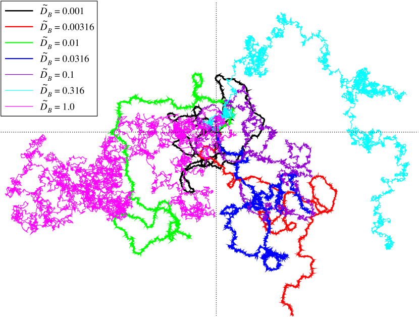
Figure 1: (Color online) Single particle trajectories for different values of $\widetilde{D}_{B}=0.001,\,0.00316,\,0.01,\,0.0316,\,0.1,\,0.316,\,1.0$. Data is generated by solving Eq. (1) during $10^{4}$ time steps, the initial position is chosen at the origin while the initial orientation is drawn from a uniform distribution in $[0,2\pi)$.

In Fig. 1 seven single-particle trajectories are presented to show the effect of varying $\widetilde{D}_{B}.$ The persistence effects are conspicuous for small values of $\widetilde{D}_{B}$ (thick curves).

An equation for the one particle probability density $P({\bm{x}},\varphi,t)\equiv\langle\delta({\bm{x}}-{\bm{x}}(t))\delta(\varphi-\varphi(t))\rangle$ can be derived by differentiating this $P({\bm{x}},\varphi,t)$ with respect to time, namely

$$\frac{\partial}{\partial t}P({\bm{x}},\varphi,t)+U_{0}\hat{\bm{u}}\cdot\nabla P({\bm{x}},\varphi,t)=\\ -\frac{\partial}{\partial\varphi}\langle\xi_{R}(t)\delta({\bm{x}}-{\bm{x}}(t))\delta(\varphi-\varphi(t))\rangle\\ -\nabla\cdot\langle\bm{\xi}_{T}(t)\delta({\bm{x}}-{\bm{x}}(t))\delta(\varphi-\varphi(t))\rangle,$$ (2)

where $\langle\cdot\rangle$ denotes the average over translational and rotational noise realizations and $\nabla=(\partial/\partial x,\partial/\partial y).$ By using Novikov’s theorem, we obtain the following Fokker-Planck equation for an active Brownian particle

$$\frac{\partial}{\partial t}P({\bm{x}},\varphi,t)+U_{0}\,\hat{\bm{u}}\cdot\nabla P({\bm{x}},\varphi,t)=\\ D_{B}\nabla^{2}P({\bm{x}},\varphi,t)+D_{\Omega}\frac{\partial^{2}}{\partial\varphi^{2}}P({\bm{x}},\varphi,t).$$ (3)

We now start to analytically solve Eq. (3). To do so, we apply the Fourier transform to Eq. (3) and we obtain

$$\frac{\partial}{\partial t}\widetilde{P}({\bm{k}},\varphi,t)+iU_{0}\,\hat{\bm{u}}\cdot{\bm{k}}\widetilde{P}({\bm{k}},\varphi,t)=\\ -D_{B}{\bm{k}}^{2}\widetilde{P}({\bm{k}},\varphi,t)+D_{\Omega}\frac{\partial^{2}}{\partial\varphi^{2}}\widetilde{P}({\bm{k}},\varphi,t),$$ (4)

where

$$\widetilde{P}({\bm{k}},\varphi,t)=(2\pi)^{-1}\int d^{2}\bm{x}\,e^{i\bm{k}\cdot\bm{x}}\,P(\bm{x},\varphi,t),$$ (5)

and ${\bm{k}}=(k_{x},k_{y})$ denotes the Fourier wave-vector. For $U_{0}=0$, Eq. (4) has as solution the set of eigenfunctions $\{e^{-(D_{B}k^{2}+D_{\Omega}n^{2})t}e^{in\varphi}\}$ with $n$ an integer. Thus we expand $\widetilde{P}(\bm{k},\varphi,t)$ on this set, expressly

$$\widetilde{P}({\bm{k}},\varphi,t)=\frac{1}{2\pi}\sum\limits_{n=-\infty}^{\infty}\widetilde{p}_{n}({\bm{k}},t)e^{-(D_{B}k^{2}+D_{\Omega}n^{2})t}e^{in\varphi},$$ (6)

with $k=|\bm{k}|$. This expansion allows to separate the effects of translational diffusion contained in the prefactor $e^{-D_{B}k^{2}t}$ from the effects of rotational diffusion due to active fluctuations.

The coefficients of the expansion are given by

$$\widetilde{p}_{n}({\bm{k}},t)=e^{(D_{B}k^{2}+D_{\Omega}n^{2})t}\int_{0}^{2\pi}d\varphi\,\widetilde{P}({\bm{k}},\varphi,t)e^{-in\varphi}.$$ (7)

After substituting Eq. (6) in Eq. (4) and using th orthogonality of the eigenfunctions we get the following set of coupled ordinary differential equations for the $n$-th coefficient of the expansion $\widetilde{p}_{n}({\bm{k}},t),$ namely

$$\frac{d}{dt}\widetilde{p}_{n}=-\frac{U_{0}}{2}ik\,e^{-D_{\Omega}t}\left[e^{2nD_{\Omega}t}e^{-i\theta}\,\widetilde{p}_{n-1}+\right.\\ \left.e^{-2nD_{\Omega}t}e^{i\theta}\,\widetilde{p}_{n+1}\right].$$ (8)

Note that we have introduced the quantities $k_{x}\pm ik_{y}=ke^{\pm i\theta}$.

Our interest lies on $P_{0}(\bm{x},t)=\int_{0}^{2\pi}d\varphi\,P(\bm{x},\varphi,t)$, which is given by the inverse Fourier transform of $\widetilde{P}_{0}(\bm{k},t)=e^{-D_{B}k^{2}t}\widetilde{p}_{0}(\bm{k},t)$ as can be checked from Eq. (7). Let us find $\widetilde{p}_{0}$ by solving Eq. (8) when the initial condition $\widetilde{P}_{n}(\bm{k},0)=\widetilde{p}_{n}(\bm{k},0)=\delta_{n,0}/2\pi$ is considered. This initial condition corresponds to the case when the particle departs from the origin in a random direction of motion drawn from a uniform distribution in $[0,2\pi)$ and is equivalent to the initial condition $P({\bm{x}},\varphi,0)=\delta^{(2)}({\bm{x}})/2\pi$, where $\delta_{n,m}$ and $\delta^{(2)}({\bm{x}})$ denote, respectively, the Kronecker delta and the delta function.

We first deal with the solution of Eq. (8) for long times. To do so, we consider only the first three Fourier coefficients $\widetilde{p}_{n},$ i.e., those with $n=0,\,\pm 1$, later on it will be shown that the other coefficients do not contribute in this regime. From Eq. (8) the three first Fourier coefficients satisfy

$$\frac{d}{dt}\widetilde{p}_{0}=-\frac{U_{0}}{2}ik\,e^{-D_{\Omega}t}\left[e^{-i\theta}\widetilde{p}_{-1}+e^{i\theta}\widetilde{p}_{1}\right],$$ (9a)

$${\frac{d}{dt}\widetilde{p}_{\pm 1}}=-\frac{U_{0}}{2}ik\,{\left[e^{D_{\Omega}t}e^{\mp i\theta}\widetilde{p}_{0}+e^{-3D_{\Omega}t}e^{\pm i\theta}\widetilde{p}_{\pm 2}\right],}$$ (9b)

which after some algebra are combined into a single equation for $\widetilde{p}_{0}$, that is

$$\frac{d^{2}}{dt^{2}}\widetilde{p}_{0}+D_{\Omega}\frac{d}{dt}\widetilde{p}_{0}=-\frac{U_{0}^{2}}{2}k^{2}\widetilde{p}_{0}\\ -\frac{U_{0}^{2}}{4}k^{2}e^{-4D_{\Omega}t}\left(e^{2i\theta}\widetilde{p}_{2}+e^{-2i\theta}\widetilde{p}_{-2}\right).$$ (10)

At this stage we argue that in the long time regime we may neglect the second term in the rhs of Eq. (10). This approximation leads to the telegrapher’s equation

$$\frac{d^{2}}{dt^{2}}\widetilde{p}_{0}+D_{\Omega}\frac{d}{dt}\widetilde{p}_{0}=-\frac{U_{0}^{2}}{2}k^{2}\widetilde{p}_{0},$$ (11)

which is rotationally symmetric in the $\bm{k}$-space and therefore, giving rise to rotationally symmetric solutions in spatial coordinates if initial conditions with the same symmetry are chosen. One may check that Eq. (11) has the solution

$$\widetilde{p}_{0}(\bm{k},t)=\widetilde{p}_{0}(\bm{k},0)\,e^{-D_{\Omega}t/2}\left[\frac{D_{\Omega}}{2\omega_{k}}\sin\omega_{k}t+\cos\omega_{k}t\right],$$ (12)

with $\omega_{k}^{2}\equiv U_{0}^{2}k^{2}/2-D_{\Omega}^{2}/4$. Therefore, by using this result one can explicitly write that $\widetilde{P}_{0}(\bm{k},t)=e^{-D_{B}{k}^{2}t}\widetilde{p}_{0}(\bm{k},t),$ with $e^{-D_{B}{k}^{2}t}$ being the translational diffusion propagator. The solution in spatial coordinates, $P_{0}(\bm{x},t)$, is obtained after taking the inverse Fourier transform of $\widetilde{P}_{0}(\bm{k},t)$, which is given by the convolution of the translational propagator with the probability distribution that retain the effects of active diffusion, i.e.,

$$P_{0}(\bm{x},t)=\int d^{2}\bm{x}^{\prime}G\left(\bm{x}-\bm{x}^{\prime},t\right)p_{0}(\bm{x}^{\prime},t),$$ (13)

where $p_{0}(\bm{x},t)$ is the inverse Fourier transform of $\widetilde{p}_{0}(\bm{k},t)$ and

$$G\left(\bm{x},t\right)=\frac{e^{-\bm{x}^{2}/4D_{B}t}}{4\pi D_{B}t},$$ (14)

is the Gaussian propagator of translational diffusion in two dimensions.

In the asymptotic limit ($t\rightarrow\infty$), at which the coherent wave-like behavior related to the second order time derivative in Eq. (11) can be neglected (mainly due to the random dispersion of the particles direction of motion), $p_{0}(\bm{x},t)$ tends to a Gaussian distribution with diffusion constant $U_{0}^{2}/2D_{\Omega}$, namely

$$p_{0}(\bm{x},t)\xrightarrow[t\rightarrow\infty]{}\frac{e^{-\bm{x}^{2}/4\left(U_{0}^{2}/2D_{\Omega}\right)t}}{4\pi\left(U_{0}^{2}/2D_{\Omega}\right)t}.$$ (15)

Substitution of this last expression into Eq. (13) and performing the integral, one gets in the long-time regime

$$P_{0}(\bm{x},t)=\frac{e^{-\bm{x}^{2}/4\left(D_{B}+U_{0}^{2}/2D_{\Omega}\right)t}}{4\pi\left(D_{B}+U_{0}^{2}/2D_{\Omega}\right)t},$$ (16)

from which the classical effective diffusion constant $D=D_{B}+U_{0}^{2}/2D_{\Omega}$ is deduced Palacci et al. (2010).

In the short time regime $D_{\Omega}t\ll 1$, we approximate $\widetilde{p}_{0}(\bm{k},t)\approx\widetilde{p}_{0}(\bm{k},0)=(2\pi)^{-1}$ and the p.d.f. in spatial coordinates corresponds to the Gaussian

$$P_{0}(\bm{x},t)\approx\frac{1}{2\pi}\frac{e^{-\bm{x}^{2}/4D_{B}t}}{4\pi D_{B}t}.$$ (17)

Though it is a difficult task to obtain from Eq. (13) the explicit dependence on $\bm{x}$ and $t$ of $P_{0}$, a formula in terms of a series expansion of the operator $\nabla^{2}$ applied to $G(\bm{x},t)$ can be derived, to say

$$P_{0}(\bm{x},t)=\frac{1}{2\pi}e^{-D_{\Omega}t/2}\sum_{s=0}^{\infty}\frac{1}{(2s)!}\left(1+\frac{D_{\Omega}t}{2}\frac{1}{2s+1}\right)\times\\ \left(\frac{D_{\Omega}t}{2}\right)^{2s}\left(1+\frac{2U_{0}^{2}}{D_{\Omega}^{2}}\nabla^{2}\right)^{s}\,G(\bm{x},t),$$ (18)

Note that the last formula can be rewritten in terms of $\partial_{t}$ instead of $\nabla^{2}$ by using that $\nabla^{2}G=D_{B}^{-1}\partial_{t}G.$

In figure 2 snapshots of the positions of $10^{5}$ particles taken at different times from numerical simulations, and for the inverse Péclet number $\widetilde{D}_{B}=0.001$, are shown. The first panel from left ($D_{\Omega}t=0.01$), corresponds to a p.d.f. close to the Gaussian given by Eq. (17). Note the formation of a rotationally symmetric ring-like structure at the intermediate time $D_{\Omega}t=0.1$ (second panel from left), mainly due to the persistence effects on the particles’ motion. The structure fades out with time (third and fourth panels from left) and starts turning into the Gaussian distribution [Eq. (16)], as time passes (far right panel for $D_{\Omega}t=100$). We must mention that in spite of the good agreement in the short and asymptotic limits given by (18), this solution does not provide an adequate description of the particles distribution in the intermediate time regime for all values of $\widetilde{D}_{B}$, particularly for the small ones, for which the effects of persistence are conspicuously prominent. The reason of this failure lies, not in the general solution (13) but in the approximated equation (11), which corresponds to the two dimensional telegrapher’s. The solution to this equation [(12)] can not be interpreted as a p.d.f. since becomes negative at short times Porr et al. (1997). This undesired feature, results from the wake effect, characteristic of the solution of the two dimensional wave equation Sevilla and Nava (2014). Notwithstanding this and as is shown later on, the mean-square displacement computed from our approximation coincides with the exact one computed from numerical simulations, at all time regimes.

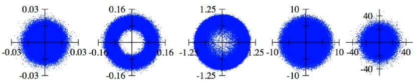
Figure 2: (Color online) Snapshots of the positions of $10^{5}$ particles taken at different times, namely from left to right, $D_{\Omega}t=0.01,\,0.1,\,1.0,\,10,$ and 100, for an inverse Péclet number $\widetilde{D}_{B}=0.001$. Notice the formation of a rotationally symmetric ring-like structure (second panel from left) that develops from a Gaussian distribution (far left panel) due to the effects of persistence in the motion of the particles. The structure fades out as time passes (third and fourth panels from left) to reach a Gaussian distribution at long times (far right panel) .

III Mean-Square Displacement

What are the effects of self-propulsion on the diffusive behavior of the system is a question that has been addressed in several experimental and theoretical studies, and the msd, being a measure of the covered space as a function of time by the random particle, has been of physical relevance in both contexts. Indeed, the msd is obtained in many experimental situations that consider active particles Selmeczi et al. (2005); ten Hagen et al. (2011a); Zheng et al. (2013), hence a way of validating existing theoretical approaches. On the other hand, it is known that the diffusion coefficient of active particles depends on the particle density, due mainly to excluded volume effects of the particles. Here we assume an enough diluted system to neglect those effects.

In what follows, an exact analytical expression for the msd will be obtained. From Eq. (11) one can show that in the coordinate space $P_{0}(\bm{x},t)$ satisfies

$$\frac{\partial^{2}}{\partial t^{2}}P_{0}+D_{\Omega}\frac{\partial}{\partial t}P_{0}=\left(\frac{U_{0}^{2}}{2}+D_{B}D_{\Omega}\right)\nabla^{2}P_{0}\\ +D_{B}\left(2\frac{\partial}{\partial t}-D_{B}\nabla^{2}\right)\nabla^{2}P_{0}.$$ (19)

If last equation is multiplied by $\bm{x}^{2}$ an integrated over the whole space, we obtain for the msd the equation

$$\frac{d^{2}}{dt^{2}}\langle\bm{x}^{2}(t)\rangle+D_{\Omega}\frac{d}{dt}\langle\bm{x}^{2}(t)\rangle=2U_{0}^{2}+4D_{B}D_{\Omega},$$ (20)

whose solution can be easily found, namely

$$\langle\bm{x}^{2}(t)\rangle=4\frac{D_{B}}{D_{\Omega}}\left(1-e^{-D_{\Omega}t}\right)\\ +\frac{2\left(2D_{B}D_{\Omega}+U_{0}^{2}\right)}{D_{\Omega}^{2}}\left[D_{\Omega}t-\left(1-e^{-D_{\Omega}t}\right)\right],$$ (21)

where we have used that $\left(d/dt\right)\left.\langle\bm{x}^{2}(t)\rangle\right|_{t=0}=4D_{B}$ in this case.

The linear dependence on time of the msd, expected in the Gaussian regime, is checked straightforwardly from Eq. (21). In the long-time regime we get

$$\langle\bm{x}^{2}(t)\rangle\xrightarrow[D_{\Omega}t\rightarrow\infty]{}4\left(D_{B}+\frac{U_{0}^{2}}{2D_{\Omega}}\right)t,$$ (22)

which is a classical result indicating that the effective diffusion of a self-propelled particle is enhanced by its activity Berg (1993). In the opposite limit.

$$\left\langle\bm{x}^{2}(t)\right\rangle\xrightarrow[D_{\Omega}t\rightarrow 0]{}4D_{B}t,$$ (23)

which once again the latter equation shows, the linear behavior with time of the msd.

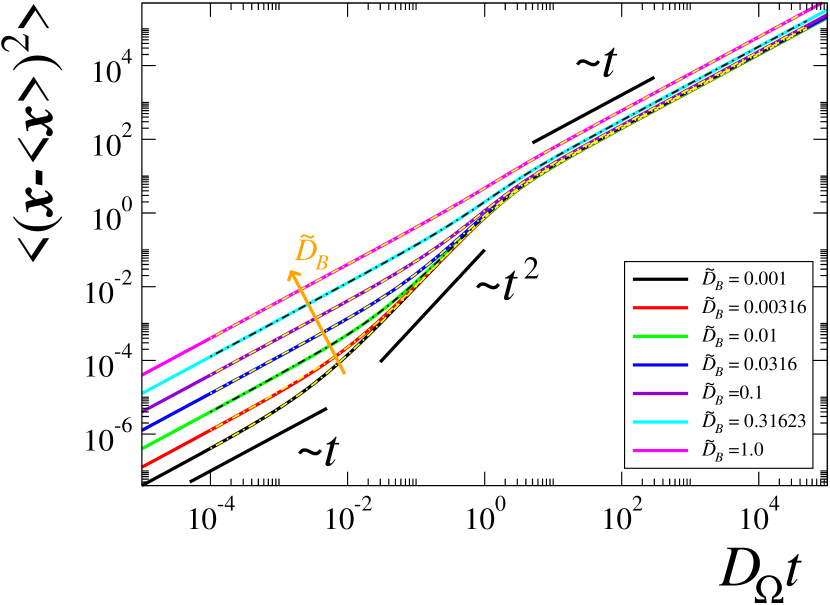
Figure 3: (Color online) Mean-square displacement in units of $U_{0}^{2}/D_{\Omega}^{2}$ as function of the dimensionless time $D_{\Omega}t$ for different values of the inverse Péclet number $\widetilde{D}_{B}$, namely 0.001, 0.0031, 0.01, 0.0316, 0.1, 0.3162, 1.0. Solid lines correspond to the analytical expression given by Eq. (21), while the thin, dash-dotted lines correspond to the results obtained from numerical simulations (see text).

III.1 Comparison of the mean-square displacement

In this subsection we compare the results obtained for the msd at short and long times using Eq. (19) with results obtained following our new Fourier approach.

For long times and with the explicit expression for $P_{0}(\bm{x},t)$ [Eq. (16)], we use the definition of the mean-square displacement, $\langle\bm{x}^{2}(t)\rangle=\int d^{2}\bm{x}\,\bm{x}^{2}P_{0}(\bm{x},t)$ to easily recover Eq. (22). For short times, we expand $\widetilde{P}_{0}(\bm{k},t)$ in powers of $k$, and we keep only the quadratic terms in $k$ for the reason that will be clear immediately afterwards, we have

$$\widetilde{P}_{0}(\bm{k},t)=1+\left(\frac{D_{\Omega}}{2}-D_{B}k^{2}\right)t-\left(\frac{D_{B}D_{\Omega}k^{2}}{2}+\frac{\omega_{k}^{2}}{2}\right)t^{2}.$$ (24)

We now use that

$$\left\langle\bm{x}^{2}(t)\right\rangle=-\nabla_{{\bm{k}}}^{2}\left.\widetilde{P}_{0}(\bm{k},t)\right|_{{\bm{k}}=0}=-\frac{1}{k}\frac{\partial}{\partial k}k\frac{\partial}{\partial k}\left.\widetilde{P}_{0}(\bm{k},t)\right|_{k=0},$$ (25)

hence, at short times, the msd of the active particle is finally given by

$$\left\langle\bm{x}^{2}(t)\right\rangle\approx 4D_{B}t+\left(2D_{B}D_{\Omega}+U_{0}^{2}\right)t^{2},$$ (26)

which shows linear and quadratic behavior of the msd. In the limit $t\rightarrow 0$, the above equation reduces to Eq. (23). Thus we have arrived to the same results by two distinct methods, namely, one method that obtained the explicit expression for the probability density and used it, and the second method that extracted information from Eq. (19) without solving it.

In order to validate our theoretical findings, we have also performed Brownian dynamics simulations. Fig. 3 shows a comparison among our theoretical prediction for any time given by Eq. (21) (solid lines), and our Brownian dynamics simulations (dashed lines) implemented to solve Eqs. (1) and averaging over 10⁵ trajectories. Each plotted line corresponds to different values of $\widetilde{D}_{B}$. We observe and excellent agreement among theory and Brownian simulations. Additionally, Fig. 3 indicates that a transition of the msd from a linear to a quadratic behavior is not always the case. For large values of $\widetilde{D}_{B}$ the linear behavior over time dominates, whereas for $\widetilde{D}_{B}$ smaller than $0.3$, a transition starts to occur. The absence of a transition from a linear to a quadratic behavior has also been reported by ten Hagen et al. ten Hagen et al. (2011a). They suggest that at short times, the msd of a self-propelled particle is affected by the initial orientation and the magnitude of its force propulsion that make that a transition occur or not.

IV Kurtosis

Once we have obtained approximately $P_{0}(\bm{x},t)$ from Eq. (3), we wish to characterize its departure from a Gaussian p.d.f. as a function of time. This quantity has been measured experimentally is systems of Janus particles To this purpose we calculate its kurtosis $\kappa$, given explicitly by Mardia (1974)

$$\kappa=\left\langle\left[(\bm{x}-\langle\bm{x}\rangle)^{T}\Sigma^{-1}(\bm{x}-\langle\bm{x}\rangle)\right]^{2}\right\rangle,$$ (27)

where $\bm{x}^{T}$ denotes the transpose of the vector $\bm{x}$ and $\Sigma$ is the $2\times 2$ matrix defined by the average of the dyadic product $(\bm{x}-\langle\bm{x}\rangle)^{T}\cdot(\bm{x}-\langle\bm{x}\rangle).$ In addition, it can be shown that for circularly symmetric distributions, as the ones considered in the present study, Eq. (27) reduces to

$$\kappa=4\frac{\langle\bm{x}^{4}(t)\rangle_{r}}{\langle\bm{x}^{2}(t)\rangle_{r}^{2}},$$ (28)

here $\langle\bm{\cdot}\rangle_{r}$ stands for the radial average over the radial probability density distribution,  namely $\langle\bm{\cdot}\rangle_{rad}=\int_{0}^{\infty}dr\,rP(r)(\cdot).$ The analytical results obtained for the kurtosis will also be compared with those obtained from numerical simulations.

As we can see, Eq. (28) requires the calculation of the fourth moment. After certain algebraic steps (see appendix B), we explicitly find that the fourth moment is given by

$$\langle\bm{x}^{4}(t)\rangle_{r}=2^{5}\frac{U_{0}^{4}}{D_{\Omega}^{4}}e^{-D_{\Omega}t/2}\left\{\left[-3\frac{D_{\Omega}t}{2}+\left(\frac{D_{\Omega}t}{2}\right)^{2}\left(1+4\widetilde{D}_{B}(1+\widetilde{D}_{B})\right)\right]\cosh\left(\frac{D_{\Omega}t}{2}\right)+\right.\\ \left.\left[3-\frac{D_{\Omega}t}{2}(1+4\widetilde{D}_{B})+\left(\frac{D_{\Omega}t}{2}\right)^{2}(1+4\widetilde{D}_{B}(1+\widetilde{D}_{B}))\right]\sinh\left(\frac{D_{\Omega}t}{2}\right)\right\}.$$ (29)

The latter analytical expression is used in Fig. 4 to plot the kurtosis, to be precise, the ratio of Eq. (29) to the square of Eq. (21). In this figure, kurtosis is plotted as a function of the dimensionless time $D_{\Omega}t$ for different values of $\widetilde{D}_{B}$ (dashed lines), while the corresponding exact results from Brownian dynamics simulations are shown in symbols. Note that for these last ones, $4\leq\kappa\leq 8$.

We observe that the kurtosis shows a clear non-monotonic behavior for $\widetilde{D}_{B}\lesssim 1$, namely, it starts to diminish from $\kappa=8$ as time passes, until it reaches a minimum at a time around $D_{\Omega}^{-1}$ that depends on the inverse of the Péclet number $\widetilde{D}_{B}$. This behavior has been observed in experiments with Janus particles in three dimensions Zheng et al. (2013) and theoretically predicted in one quasi-one-dimensional channels ten Hagen et al. (2009). In the limit of vanishing translational diffusion, the kurtosis is a monotonic increasing function of time, with $\kappa=4$ as its minimum value Sevilla and Nava (2014). At later times the kurtosis starts to increase reaching the value 8 in the asymptotic limit. This behavior becomes less and less evident as the translational diffusion coefficient surpasses the effective diffusion coefficient that originates in the rotational diffusion, $U_{0}^{2}/D_{\Omega}.$ Due to this effect, we note a better agreement between our analytical approximation and our simulation results, as $\widetilde{D}_{B}$ is increased. On the other hand, the persistence effects induced by orientational correlations are revealed in the diminishing regime of the kurtosis, as is shown in Fig. 4 for the cases in which $\widetilde{D}_{B}\lesssim 1$ (see Table 1 for the values of $\kappa$ corresponding to the snapshots shown in Fig. 2). In this regime the orientational correlations surpass the effects of translational noise hence allowing the particles to move persistently outwardly from the origin and giving rise to circularly-symmetric, ring-like distributions as the one shown in Fig. 2 (second from left) at $D_{\Omega}t=0.1$ for $\widetilde{D}_{B}=0.001$. Afterwards, this ring-like distributions turns into a Gaussian distribution as the orientational correlations die out. Notice that the discrepancy between the results given by our analytical approximation and the exact results lies on the wave-like effects given by the second-order-time-derivative term of Eq. (11) which, as shown in Sevilla and Nava (2014), gives $8/3\simeq 2.6667$ as the value for the kurtosis in the vanishing translational diffusion. For $\widetilde{D}_{B}=0.001$, the minimum of the exact kurtosis is about $4.1352$ at $t\approx 0.39D_{\Omega}^{-1}$ while from our analytical approximate $\kappa\approx 3.0184$ at $t\approx 0.239D_{\Omega}^{-1}$.

In the next subsections we find asymptotic expression for the kurtosis for both short and long times that confirm the Gaussianity of the distribution function for these time regimes.

Table 1: Kurtosis values at times $D_{\Omega}t$ that are close to those values chosen in Fig. 2 ($\widetilde{D}_{B}=0.001$).

$D_{\Omega}t$	$0.01$	$0.1$	$1.01$	$10.245$	$100.08$
$\kappa$	$5.9598$	$4.3111$	$4.2729$	$6.7621$	$7.8713$

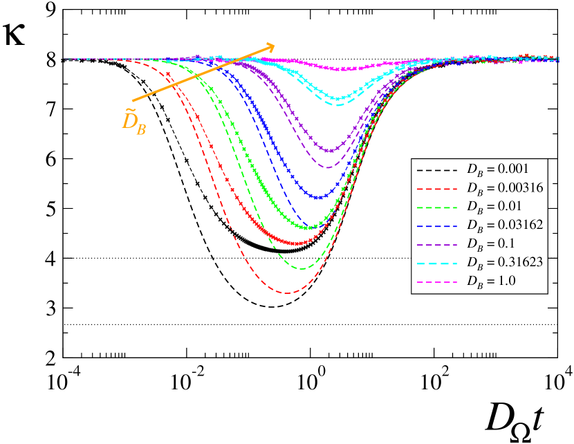
Figure 4: (Color online) Kurtosis of the particles distribution as function of the dimensionless time $D_{\Omega}t$ for different values of $\widetilde{D}_{B}$, namely 0.001, 0.0031, 0.01, 0.0316, 0.1, 0.3162, 1.0. Dashed lines correspond to the exact analytical expression given by the quotient of Eq. (29) and Eq. (21), while the symbols mark the values of the kurtosis obtained from numerical simulations. Thin-dotted lines mark the values 8, 4, 8/3, that correspond respectively in two dimensions to: a Gaussian distribution, a ring-like distribution and wave-like distribution Sevilla and Nava (2014).

IV.1 Kurtosis at short times

In ordet to find $\kappa$ for $t\rightarrow 0,$ we expand $\widetilde{P}_{0}(\bm{k},t)$ in a power series in $k$, use the fact that $\omega_{k}^{2}\equiv U_{0}^{2}k^{2}/2-D_{\Omega}^{2}/4$, and keep terms only of order $k^{4}$ to get

$$\widetilde{P}_{0}(\bm{k},t) \approx k^{4}\left[\frac{D_{\Omega}}{2}\frac{c^{4}t^{5}}{5!}+\frac{c^{4}t^{4}}{4!}+\frac{D_{\Omega}}{2}\frac{c^{2}D_{B}t^{4}}{3!}\right.$$ (30)

$$\left.+\frac{c^{2}D_{B}t^{3}}{2}+\frac{D_{\Omega}D_{B}^{2}t^{3}}{4}+\frac{D_{B}^{2}t^{2}}{2}\right],$$

$$= k^{4}f(t).$$

We now use Eq. (44), that together with Eq. (26), one finally gets for short times that

$$\kappa\approx\frac{4^{3}f(t)}{\left(4D_{B}t+2D_{B}D_{\Omega}t^{2}+U_{0}^{2}t^{2}\right)^{2}}=8,$$ (31)

which means that our derived p.d.f. has a Gaussian behavior at short times. This result has been validated numerically and illustrated in Fig. 4, where kurtosis is plotted versus time. It clearly can be seen that for short times $\kappa$ has a value of $8$.

IV.2 Kurtosis at long times

In ordet to find $\kappa$ for $t\rightarrow\infty,$ we proceed as before, we expand $P\widetilde{P}_{0}(\bm{k},t)$ in power series of $k$, use that $\omega_{k}^{2}\equiv U_{0}^{2}k^{2}/2-D_{\Omega}^{2}/4$, but now keep all the terms in the series expansion. After applying Eq. (44) we get that in the long time limit

$$\langle\bm{x}^{4}(t)\rangle \approx \frac{2^{5}U_{0}^{4}}{D_{\Omega}^{4}}\left[1+\frac{4D_{B}D_{\Omega}}{U_{0}^{2}}\right.$$ (32)

$$\left.+4\left(\frac{D_{B}D_{\Omega}}{U_{0}^{2}}\right)^{2}\right]\left(\frac{D_{\Omega}t}{2}\right)^{2}.$$

Finally we use Eq. (22) to get for long times that

$$\kappa=\frac{\langle\bm{x}^{4}(t)\rangle}{4\left(D_{B}+\frac{U_{0}^{2}}{2D_{\Omega}}\right)t}=8,$$ (33)

which once again, Eq. (33) shows that kurtosis has a Gaussian behavior for long times. This result has also been validated using Brownian dynamics and shown in Fig. 4, where for long values of the dimensionless time, $\kappa$ tends again to a value of $8$.

V The active flux: the velocity field $\bm{V}(\bm{x},t)$ of active particles

The Fourier expansion given by Eq. (6) allows us to obtain the hydrodynamic fields. At the moment we have explicitly calculated $\widetilde{P}_{0}(\bm{k},t)$ that corresponds to the Fourier transform of the density field $\rho(\bm{x},t)$. The Fourier transform of the components of the velocity field $\bm{V}(\bm{x},t)$ are related to $\widetilde{p}_{\pm 1}(\bm{k},t)$ in the following way. By definition

$$\widetilde{V}_{x}(\bm{k},t) =U_{0}\int_{0}^{2\pi}d\varphi\,\cos\varphi\widetilde{P}(\bm{k},\varphi,t),$$ (34a)

$$\widetilde{V}_{y}(\bm{k},t) =U_{0}\int_{0}^{2\pi}d\varphi\,\sin\varphi\widetilde{P}(\bm{k},\varphi,t),$$ (34b)

and after substitution of Eq. (6) in Eq. (34) we get

$${\widetilde{V}_{x}}(\bm{k},t)= \frac{U_{0}}{2}\,e^{-(D_{B}k^{2}+D_{\Omega})t}\,\left[\widetilde{p}_{1}(\bm{k},t)+\widetilde{p}_{1}^{*}(-\bm{k},t)\right],$$ (35a)

$${\widetilde{V}_{y}}(\bm{k},t)= \frac{U_{0}}{2}\,e^{-(D_{B}k^{2}+D_{\Omega})t}\,\left[\widetilde{p}_{1}^{*}(-\bm{k},t)-\widetilde{p}_{1}(\bm{k},t)\right],$$ (35b)

where we have used that $\widetilde{p}_{-n}(\bm{k},t)=\widetilde{p}_{n}^{*}(-\bm{k},t).$ With these expressions, it is straightforward to verify that Eq. (9a) corresponds to the continuity equation $\partial_{t}\rho+\nabla\cdot\bm{V}(\bm{x},t)=0.$ At the long time regime, where only the first three Fourier modes are needed, we have that $\widetilde{p}_{1}(\bm{k},t)$ can be computed from Eq. (12) if we neglect the term that involves $p_{2},$ i.e., from

$${\frac{d}{dt}\widetilde{p}_{1}}=-\frac{U_{0}}{2}ike^{-i\theta}\,e^{D_{\Omega}t}\widetilde{p}_{0}.$$ (36)

We now use the explicit expression for $\widetilde{p}_{0}$, that is Eq. (12), with $\widetilde{p}_{0}(\bm{k},0)=1/(2\pi)$ to integrate Eq. (36). After some steps we find that

$$\widetilde{p}_{1}(\bm{k},t)=-\frac{U_{0}}{4\pi}\left(ik_{x}+k_{y}\right)e^{D_{\Omega}t/2}\frac{\sin\omega_{k}t}{\omega_{k}}.$$ (37)

If we insert the latter into Eqs. (35a)-(35b) we obtain

$$\widetilde{V}_{x}(\bm{k},t) = -\frac{U_{0}^{2}}{4\pi}ik_{x}e^{-\left(D_{B}k^{2}+D_{\Omega}/2\right)t}\frac{\sin\omega_{k}t}{\omega_{k}},$$

$$\widetilde{V}_{y}(\bm{k},t) = -\frac{U_{0}^{2}}{4\pi}ik_{y}e^{-\left(D_{B}k^{2}+D_{\Omega}/2\right)t}\frac{\sin\omega_{k}t}{\omega_{k}}.$$

After inverting the Fourier transform, this pair of expressions can be brought into the form

$$\bm{V}(\bm{x},t)=-\frac{U_{0}^{2}}{2}\nabla F(\bm{x},t),$$ (38)

where the function $F(\bm{x},t)$ depends on $P_{0}$, explicitly

$$F(\bm{x},t)=\int_{0}^{t}ds\,e^{D_{\Omega}(t-s)}\int d^{2}\bm{x}^{\prime}G(\bm{x}-\bm{x}^{\prime},t-s)P_{0}(\bm{x}^{\prime},s).$$ (39)

Last expression corresponds to a non-Fickian constitutive relation that considers nonlocal effect in space and time. This relation, together with the continuity equation, gives rise to a non-local (in both, space and time) diffusion-like equation.

In a similar way, one can systematically find higher Fourier modes for the probability density function, $\widetilde{P}({\bm{k}},\varphi,t)$, in the wave vector space.

VI Final Comments and Conclusions

Though Eq. (21) has been derived from the long time approximation, it does give the correct time dependence at all times as it is shown in Fig. 3, where our analytical formula (solid lines) is compared against numerical simulations (dashed lines). This fact can be understood directly from Eq. (10), since it can be shown that the inhomogeneous term does not contribute to the mean squared displacement (see appendix A), therefore agreeing with the expression obtained from the telegrapher’s Eq. (11).

We want to point out that though the linear time dependence of the msd, characteristic of normal diffusion, is reached at times $D_{\Omega}t\sim 1$ (see Fig. 3), the Gaussian behavior of the distribution is reached at much later times (see Fig. 4), suggesting that at finite times, $D_{\Omega}t>1$, normal diffusion does strictly corresponds to Gaussian distributions. The kurtosis computed from our approximation shows that it tends asymptotically to Gaussian, $\kappa=8$, as $(8-D_{\Omega}t)^{-1}$. In contrast, in the short time regime, the distribution departs from a Gaussian behavior with time as $(8-D_{\Omega}t)^{-2}$ (see Fig. 5).

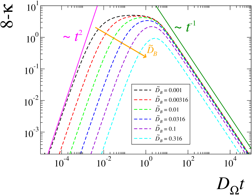
Figure 5: (Color online) The departure from Gaussian behavior of $P_{0}(\bm{x},t),$ measured by $8-\kappa$, differs in the short-time regime from the long-time regime. In the first case the departure captured by the power law $(D_{\Omega}t)^{-2}$ while in the long-time regime such departure is well described simply by $(D_{\Omega}t)^{-1}$.

In summary, we have found a method and obtained with it, an analytical solution to the Smoluchowski equation of an active Brownian particle self-propelling with a constant velocity. We used a Fourier approach and exploited the circular symmetry of the distribution function, to obtain an infinite system of coupled ordinary differential equations for the Fourier modes of the probability density. Our formalism showed that in order to have a whole description for the particles diffusion, we only need the first Fourier coefficient, since it was found that higher Fourier modes do not contribute to the mean-square displacement of the particle. With the explicit p.d.f. in hand, we calculated the particle mean-square displacement for both long and short times, recovering classical results of enhanced diffusion due to activity. We also validated these findings by performing Brownian dynamics simulations that showed and excellent agreement among theory and simulations. In addition, we also performed an asymptotic analysis for short and long times, to the forth moment of our p.d.f. This calculation enabled us to have analytical results for the kurtosis. The asymptotic results for this measure were validated with Brownian dynamics simulations that showed that the p.d.f. of an active particle always starts with a Gaussian behavior, and depending on the vale of the ratio $\widetilde{D}_{B}$, it may evolve to a ring-like distribution, but it always returns to a Gaussian distribution for long times. Finally this work shed light on mathematical procedures to solve a Smoluchowski equation for an active Brownian particle.

Future venues for this research, would be to solve analytically a Smoluchowski equation for confined active particles and/or particles interacting among them.

Appendix A Mean Square Displacement

If we apply the operator $-\nabla^{2}_{\bm{k}}$ to the relation $\widetilde{P}_{0}(\bm{k},t)=e^{-D_{B}{k}^{2}t}\widetilde{p}_{0}(\bm{k},t)$ and evaluate at $\bm{k}=0$, one gets that $\langle\bm{x}^{2}(t)\rangle=4D_{B}t+\langle\bm{x}^{2}(t)\rangle_{0}$, which leads straightforwardly to the pair of relations

$$\frac{d^{2}}{dt^{2}}\langle\bm{x}^{2}(t)\rangle =\frac{d^{2}}{dt^{2}}\langle\bm{x}^{2}(t)\rangle_{0}$$ (40a)

$$\frac{d}{dt}\langle\bm{x}^{2}(t)\rangle =4D_{B}+\frac{d}{dt}\langle\bm{x}^{2}(t)\rangle_{0},$$ (40b)

where $\langle\cdot\rangle_{0}$ denotes the average of $(\cdot)$ with $p_{0}(\bm{x},t)$ as the probability measure. The quantity $\frac{d^{2}}{dt^{2}}\langle\bm{x}^{2}(t)\rangle_{0}$ can be computed directly by applying $-\nabla^{2}_{\bm{k}}$ to Eq. (10) and evaluating at $\bm{k}=0$, which results in

$$\frac{d^{2}}{dt^{2}}\langle\bm{x}^{2}(t)\rangle_{0}+D_{\Omega}\frac{d}{dt}\langle\bm{x}^{2}(t)\rangle_{0}=\frac{U_{0}^{2}}{2}\left[\nabla^{2}_{\bm{k}}(k_{x}^{2}+k_{y}^{2})\widetilde{p}_{0}\right]_{\bm{k}=0}\\ +\frac{U_{0}^{2}}{4}e^{-4D_{\Omega}t}\left\{\nabla^{2}_{\bm{k}}\left[(k_{x}-ik_{y})^{2}\widetilde{p}_{-2}+(k_{x}+ik_{y})^{2}\widetilde{p}_{2}\right]\right\}_{\bm{k}=0}$$ (41)

It is easy to show that the first term of rhs of the last equation is $2U_{0}^{2}$ while the next term, that involves the modes $\widetilde{p}_{\pm 2}$ vanishes identically, thus we get

$$\frac{d^{2}}{dt^{2}}\langle\bm{x}^{2}(t)\rangle_{0}+D_{\Omega}\frac{d}{dt}\langle\bm{x}^{2}(t)\rangle_{0}=2U_{0}^{2},$$ (42)

and therefore, using Eqs. (40) we finally have that

$$\frac{d^{2}}{dt^{2}}\langle\bm{x}^{2}(t)\rangle+D_{\Omega}\frac{d}{dt}\langle\bm{x}^{2}(t)\rangle_{0}=2U_{0}^{2}+4D_{B}D_{\Omega},$$ (43)

which coincides with Eq. (20), deduced from the telegrapher Eq. (11) when considering only the first three Fourier modes $\widetilde{p}_{0}\,,\widetilde{p}_{\pm 1}$.

Appendix B Calculation of the Fourth moment of $P_{0}(\bm{x},t)$

The fourth moment $\langle\bm{x}^{4}(t)\rangle_{r}$ can be obtained through the prescription

$$\langle\bm{x}^{4}(t)\rangle=\left(\frac{1}{k}\frac{\partial}{\partial k}k\frac{\partial}{\partial k}\right)^{2}\left.\widetilde{P}_{0}(\bm{k},t)\right|_{k=0}.$$ (44)

Though it is possible to use this prescription directly on $\widetilde{P}_{0}(\bm{k},t)$, we prefer to apply it to the series expansion in powers of $k$ of $\widetilde{P}_{0}(\bm{k},t)$, this is due to the complicated dependence of $\widetilde{P}_{0}$ on $k$. Such expansion is given by

$$\widetilde{P}_{0}(\bm{k},t)=e^{-D_{\Omega}t/2}\sum_{n,m=0}^{\infty}\sum_{j=0}^{m}\binom{m}{j}\frac{(-D_{B}t)^{n}}{n!}\frac{(it)^{2m}}{(2m)!}\\ \times\left(1+\frac{D_{\Omega}t}{2(2m+1)}\right)\left(-\frac{D_{\Omega}^{2}}{4}\right)^{m-j}\left(\frac{U_{0}^{2}}{2}\right)^{j}\,k^{2(n+j)}.$$ (45)

where we have used the explicit dependence on $k$, of $\omega_{k},$ given in section II.

Since

$$\left(\frac{1}{k}\frac{\partial}{\partial k}k\frac{\partial}{\partial k}\right)^{2}k^{2(n+j)}=\left[2(n+j)\right]^{2}\times\\ \left[2(n+j-1)\right]^{2}k^{2(n+j-2)},$$ (46)

the only terms that survives when evaluating at $k=0$ are those for which $n+j=2$ with the condition that $0\leq j\leq m$. Thus we can write

$$\langle\bm{x}^{4}(t)\rangle=4^{4}\frac{U_{0}^{4}}{D_{\Omega}^{4}}e^{-D_{\Omega}t/2}\sum_{m=0}^{\infty}\left(\frac{D_{\Omega}t}{2}\right)^{2m+2}\left[\left(\frac{D_{\Omega}t}{2}\right)^{2}\left(1+\frac{D_{\Omega}t}{2}\frac{1}{2m+5}\right)\frac{(m+2)(m+1)}{2(2m+4)!}+\right.\\ \widetilde{D}_{B}\left(\frac{D_{\Omega}t}{2}\right)\left(1+\frac{D_{\Omega}t}{2}\frac{1}{2m+3}\right)\frac{m+1}{(2m+2)!}+\widetilde{D}_{B}^{2}\left.\left(1+\frac{D_{\Omega}t}{2}\frac{1}{2m+1}\right)\frac{1}{2(2m)!}\right]$$ (47)

The sums can be written in terms of hyperbolic function, and after some algebraic steps Eq. (29) is recovered.

References

- Lovely and Dahlquist (1975) P. S. Lovely and F. W. Dahlquist, J. Theor. Biol. 50, 477 (1975).
- Pedley and Kessler (1992) T. J. Pedley and J. O. Kessler, Annu. Rev. Fluid Mech. 24, 313 (1992).
- Berg (1993) H. C. Berg, Random walks in biology (Princeton University Press, Princeton, N. J., 1993).
- Ishikawa and Pedley (2007) T. Ishikawa and T. Pedley, J. Fluid Mech. 588, 437 (2007).
- Howse et al. (2007) J. R. Howse, R. A. L. Jones, A. J. Ryan, T. Gough, R. Vafabakhsh, and R. Golestanian, Phys. Rev. Lett. 99, 048102 (2007).
- Romanczuk et al. (2012) P. Romanczuk, M. Bar, W. Ebeling, B. Lindner, and L. Schimansky-Geier, Eur. Phys. J. Special Topics 202, 1 (2012).
- Lauga and Powers (2009) E. Lauga and T. Powers, Rep. Prog. Phys. 72, 096601 (2009).
- Jülicher and Prost (2009) F. Jülicher and J. Prost, The European Physical Journal E 29, 27 (2009).
- Sevilla and Nava (2014) F. J. Sevilla and L. A. Gomez Nava, Physical Review E 90, 022130 (2014).
- Fily et al. (2014) Y. Fily, A. Baskaran, and M. F. Hagan, Soft Matter 10, 5609 (2014).
- Yang et al. (2014) X. Yang, M. L. Manning, and M. C. Marchetti, Soft Matter 10, 6477 (2014).
- Abbott et al. (2009) J. J. Abbott, K. E. Peyer, M. C. Lagomarsino, L. Zhang, L. Dong, I. K. Kaliakatsos, and B. J. Nelson, Int. J. Robot. Res. 28, 1434 (2009).
- Kosa et al. (2012) G. Kosa, P. Jakab, G. Szekely, and N. Hata, Biomed. Microdevices 14, 165 (2012).
- Gao et al. (2014) W. Gao, R. Dong, S. Thamphiwatana, J. Li, W. Gao, L. Zhang, and J. Wang, ACS nano (2014).
- Mallouk and Sen (2009) T. E. Mallouk and A. Sen, Sci. Am. 300, 72 (2009).
- Paxton et al. (2006) W. F. Paxton, S. Sundararajan, T. E. Mallouk, and A. Sen, Angew. Chem., Int. Ed. 45, 5420 (2006).
- Mirkovic et al. (2010) T. Mirkovic, N. S. Zacharia, G. D. Scholes, and G. A. Ozin, ACS Nano 4, 1782 (2010).
- ten Hagen et al. (2011a) B. ten Hagen, S. van Teeffelen, and H. Lowen, J. Phys. Condens. Matter 23, 194119 (2011a).
- Lobaskin et al. (2008) V. Lobaskin, D. Lobaskin, and I. Kulic, Eur. Phys. J. Special Topics. 157, 149 (2008).
- Ebbens et al. (2010) S. Ebbens, R. A. L. Jones, A. J. Ryan, R. Golestanian, and J. R. Howse, Phys. Rev. E 82, 015304(R) (2010).
- van Teeffelen and Lowen (2008) S. van Teeffelen and H. Lowen, Phys. Rev. E 78, 020101 (2008).
- ten Hagen et al. (2011b) B. ten Hagen, R. Wittkowski, and H. Lowen, Phys. Rev. E. 84, 031105 (2011b).
- Sandoval et al. (2014) M. Sandoval, N. K. Marath, G. Subramanian, and E. Lauga, J. Fluid Mech. 742, 50 (2014).
- Pedley and Kessler (1990) T. J. Pedley and J. O. Kessler, Journal of Fluid Mechanics 212, 155 (1990), ISSN 1469-7645, URL http://journals.cambridge.org/article_S0022112090001914.
- Bearon and Pedley (2000) R. N. Bearon and T. J. Pedley, Bull. Math. Biol. 62, 775 (2000).
- Enculescu and Stark (2011) M. Enculescu and H. Stark, Phys. Rev. Lett. 107, 058301 (2011), URL http://link.aps.org/doi/10.1103/PhysRevLett.107.058301.
- Pototsky and Stark (2012) A. Pototsky and H. Stark, EPL 98, 50004 (2012).
- Saintillan and Shelley (2008) D. Saintillan and M. J. Shelley, Phys. Rev. Lett. 100, 178103 (2008), URL http://link.aps.org/doi/10.1103/PhysRevLett.100.178103.
- Babel et al. (2014) S. Babel, B. ten Hagen, and H. Lowen, J. Stat. Mech. P02011, 1 (2014).
- Bazazia et al. (2008) S. Bazazia, J. Buhl, J. J. Hale, M. L. Anstey, G. A. Sword, S. J. Simpson, and I. D. Couzin, Curr. Biol. 18, 735 (2008).
- Vicsek et al. (1995) T. Vicsek, A. Czirok, E. Ben-Jacob, I. Cohen, and O. Shochet, Phys. Rev. Lett. 75, 1226 (1995).
- Romanczuk and Schimansky-Geier (2011) P. Romanczuk and L. Schimansky-Geier, Phys. Rev. Lett. 106, 230601 (2011), URL http://link.aps.org/doi/10.1103/PhysRevLett.106.230601.
- Zheng et al. (2013) X. Zheng, B. ten Hagen, A. Kaiser, M. Wu, H. Cui, Z. Silber-Li, and H. Lowen, Physical Review E 88, 032304 (2013).
- Palacci et al. (2010) J. Palacci, C. Cottin-Bizonne, C. Ybert, and L. Bocquet, Phys. Rev. Lett. 105, 088304 (2010).
- Porr et al. (1997) J. M. Porra, J. Masoliver, and G. H. Weiss, Phys. Rev. E 55, 7771 (1997), URL http://link.aps.org/doi/10.1103/PhysRevE.55.7771.
- Selmeczi et al. (2005) D. Selmeczi, S. Mosler, P. H. Hagedorn, N. B. Larsen, and H. Flyvbjerg, Biophys. J. 89, 912 (2005).
- Mardia (1974) K. V. Mardia, Sankhyā: The Indian Journal of Statistics, Series B pp. 115 – 128 (1974).
- ten Hagen et al. (2009) B. ten Hagen, S. van Teeffelen, and H. Lowen, Cond. Mat. Phys. 12, 725 (2009).