DES13S2cmm: The First Superluminous Supernova from the Dark Energy Survey

Abstract

We present DES13S2cmm, the first spectroscopically-confirmed superluminous supernova (SLSN) from the Dark Energy Survey (DES). We briefly discuss the data and search algorithm used to find this event in the first year of DES operations, and outline the spectroscopic data obtained from the European Southern Observatory (ESO) Very Large Telescope to confirm its redshift ($z=0.663\pm 0.001$ based on the host-galaxy emission lines) and likely spectral type (type I). Using this redshift, we find $M^{peak}_{U}=-21.05^{+0.10}_{-0.09}$ for the peak, rest-frame $U$-band absolute magnitude, and find DES13S2cmm to be located in a faint, low metallicity (sub-solar), low stellar-mass host galaxy ($\log(\mathrm{M}/\mathrm{M}_{\odot})=9.3\pm 0.3$); consistent with what is seen for other SLSNe-I. We compare the bolometric light curve of DES13S2cmm to fourteen similarly well-observed SLSNe-I in the literature and find it possesses one of the slowest declining tails (beyond $+30$ days rest frame past peak), and is the faintest at peak. Moreover, we find the bolometric light curves of all SLSNe-I studied herein possess a dispersion of only 0.2–0.3 magnitudes between $+25$ and $+30$ days after peak (rest frame) depending on redshift range studied; this could be important for ‘standardising’ such supernovae, as is done with the more common type Ia. We fit the bolometric light curve of DES13S2cmm with two competing models for SLSNe-I – the radioactive decay of ⁵⁶Ni, and a magnetar – and find that while the magnetar is formally a better fit, neither model provides a compelling match to the data. Although we are unable to conclusively differentiate between these two physical models for this particular SLSN-I, further DES observations of more SLSNe-I should break this degeneracy, especially if the light curves of SLSNe-I can be observed beyond 100 days in the rest frame of the supernova.

1 Introduction

The last five years have seen the emergence of a new class of ultra-bright stellar explosions: superluminous supernovae (SLSNe; for a review see Gal-Yam, 2012), some 50 times brighter than classical supernova (SN) types. Data on these rare and extreme events are still sparse, with only $\sim$50 SLSN detections reported in the literature. These events have generally been poorly studied with incomplete imaging and spectroscopy, leaving many aspects of their observational characteristics, and their physical nature, unknown.

Yet these SLSNe could play a key role in many diverse areas of astrophysics: tracing the evolution of massive stars, driving feedback in low mass galaxies at high redshift, and providing potential line-of-sight probes of interstellar medium to their high-redshift hosts (Berger et al., 2012). SLSNe have also been detected to $z\sim 4$ (Cooke et al., 2012), far beyond the reach of the current best cosmological probe, type Ia supernovae (SNe Ia). If SLSNe can be standardised (e.g. Inserra & Smartt, 2014), as is done with SNe Ia (Tripp, 1998; Phillips, 1993; Riess et al., 1996), then a new era of SN cosmology would be possible, with the potential to accurately map the expansion rate of the universe far into the epoch of deceleration (Delubac et al., 2014).

SLSNe have been divided into three possible types: SLSN-II, SLSN-I and SLSN-R (see Fig. 1 of Gal-Yam, 2012). SLSNe-II show signs of interactions with CSM via narrow hydrogen lines (e.g., Ofek et al., 2007; Smith et al., 2007), and thus may simply represent the bright end of a continuum of Type IIn SNe (although this is not well established).

SLSN-I are spectroscopically classified as hydrogen free (Quimby et al., 2011), and are possibly related to Type Ic SNe at late times (Pastorello et al., 2010), but normal methods of powering such SNe (e.g., the radioactive decay of ⁵⁶Ni or energy from the gravitational collapse of a massive star) do not appear to be able to simultaneously reproduce their extreme brightness, slowly-rising light curves, and decay rates (Inserra et al., 2013). Many alternative models have been proposed: the injections of energy into a SN ejecta via the spin down of a young magnetar (Kasen & Bildsten, 2010; Woosley, 2010; Inserra et al., 2013); interaction of the SN ejecta with a massive (3-5 M_⊙) C/O-rich circumstellar material (CSM; e.g., Blinnikov & Sorokina, 2010); or collisions between high-velocity shells generated from a pulsational pair-instability event (Woosley et al., 2007). These explanations are still actively debated in the literature.

SLSNe-R are rare and characterised by possessing extremely long, slow-declining light curves ($>200$ days in the rest frame). SLSNe-R originally appeared consistent with the death of $\gtrsim$100 M_⊙ stars via the pair instability mechanism (Gal-Yam et al., 2009). However, new observations – and the lack of significant spectral differences between SLSN-I and SLSN-R – have challenged the notion that these classes are truly distinct (Nicholl et al., 2013) and maybe better described together as Type Ic SLSNe (Inserra et al., 2013).

In summary, the origin of the power source for SLSNe (of all types) remains unclear, with the possibility that further sources of energy may be viable. A more detailed understanding requires an increase in both the quantity and quality of the data obtained on these events. However, finding more SLSNe (of any type) with existing transient searches is challenging, especially in the local universe where the rates are only $\simeq 10^{-4}$ that of the core-collapse SN rate (Quimby et al., 2013; McCrum et al., 2014) thus making it hard to assemble large samples of events over reasonable timescales, even from large surveys. For example, McCrum et al. (2014) detected only 10 SLSN candidates over $0.3\leq z\leq 1.4$ within the first year of the PanSTARRS1 Medium Deep Survey.

Searches for SLSNe at higher redshifts may be more profitable as the rates of SLSNe appear to rise by a factor of $\sim$10-15 at $z>1.5$ (Cooke et al., 2012), perhaps tracking the increased cosmic star-formation rate and/or decreasing cosmic metallicity: SLSNe are preferentially found in faint, low-metallicity galaxies (Neill et al., 2011; Chen et al., 2013; Lunnan et al., 2014). Moreover, the peak of a SLSN’s energy output is located in the UV region of the electromagnetic spectrum, which is redshifted to optical wavelengths at high redshift.

In this paper, we outline our first search for SLSNe in the Dark Energy Survey (DES). In Section 2, we discuss details of DES and our preliminary search, while in Section 3, we describe the first SLSN detected in DES and provide details of its properties, including our spectroscopic confirmation. In Section 4, we compare our SLSN to other events in the literature and explore the possible power sources for our event. We conclude in Section 5. Throughout this paper, we assume a flat $\Lambda$-dominated cosmology with $\Omega_{M}=0.28$ and $H_{0}=70$ km s^-1 Mpc^-1, consistent with recent cosmological measurements (e.g. Anderson et al., 2014; Betoule et al., 2014).

2 The Dark Energy Survey

The Dark Energy Survey (DES; Flaugher, 2005) is a new imaging survey of the southern sky focused on obtaining accurate constraints on the equation-of-state of dark energy. Observations are carried out using the Dark Energy Camera (DECam; Flaugher et al., 2012; Diehl & For the Dark Energy Survey Collaboration, 2012) on the 4-metre Blanco Telescope at the Cerro Tololo Inter-American Observatory (CTIO) in Chile. DECam was successfully installed and commissioned in 2012, and possesses a 3 deg² field-of-view with 62 fully depleted, red-sensitive CCDs.

2.1 DES Supernova Survey

DES conducted science verification (SV) observations from November 2012 to February 2013, and then began full science operations in mid-August 2013, with year one running until February 2014. DES is performing two surveys in parallel: a wide-field, multi-colour ($grizY$) survey of 5000 deg² for the study of clusters of galaxies, weak lensing and large scale structure; and a deeper, cadenced multi-colour ($griz$) search for SNe. In this paper we focus on this DES SN Survey, as outlined in Bernstein et al. (2012), which surveys 30 deg² over 10 DECam fields (two ‘deep’, eight ‘shallow’) located in the XMM-LSS, ELAIS-S, CDFS and ‘Stripe82’ regions. As of November 2014, the DES SN Survey has already discovered over a thousand SN Ia candidates, with more than 70 spectroscopic classifications to date.

This rolling search for SNe Ia is also ideal for discovering other transient phenomena including SLSNe. Using the light curve of SNLS-06D4eu (a SLSN-I; Howell et al., 2013), we calculate that DES could detect such an event to $z=2.5$ given the limiting magnitudes for the DES deep fields. For example, assuming a volumetric rate of $32\,\mathrm{Gpc}^{-3}\,\mathrm{yr}^{-1}$ from Quimby et al. (2013) and correcting for time dilation, we estimate DES should find approximately 3.5 SLSN-I events per DES season (five months) in the deep fields and many more in the shallow fields (although at a lower redshift). This basic prediction is uncertain because: i) We have not corrected for ‘edge effects’ that will reduce the number of SLSNe with significant light-curve coverage; ii) The volumetric rates themselves may evolve with redshift (e.g., Cooke et al., 2012) and have large uncertainties (McCrum et al., 2014); and iii) We have not included any corrections for survey completeness.

2.2 Selecting SLSNe candidates

We began our search for SLSNe using the data products from the DES SN Survey. All imaging data were de-trended and co-added using a standard photometric reduction pipeline at the National Center for Supercomputing Applications (NCSA) using the DES Data Management system (DESDM; Mohr et al., 2012; Desai et al., 2012), producing approximately 30 ‘search images’ per field (in all filters) over the duration of the five-month DES season. We perform difference imaging on each of these search images, using deeper template images for each field created from the co-addition of several epochs of data obtained during the SV period in late 2012. Before differencing, the search and template images were convolved to the same point spread function (PSF).

Objects were selected from the difference images using SExtractor (Bertin & Arnouts, 1996) v2.18.10, and previously unknown transient candidates were identified and examined using visual inspection (or ‘scanning’) by DES team members. Over the course of the first year of DES approximately $25,000$ new transient candidates were selected in this manner, including many data artefacts in addition to legitimate SN-like objects. A machine learning algorithm (Goldstein et al., in preparation) was used to improve our efficiency of selecting real transients. Transient candidates were photometrically classified using the Photometric SN IDentification software (PSNID; Sako et al., 2008, 2011) to determine the likely SN type based on fits to a series of SN templates. These SN candidates were stored in a database and prioritized for their spectroscopic follow-up.

During the first season of DES, PSNID only included templates for the normal SN types Ib/c, II and Ia, so a fully automated classification of SLSN candidates was not possible. Therefore, for this first season of DES, we searched for candidate SLSNe using the following criteria: i) At least one month of multi-colour data, i.e., typically five to six detections ($S/N>3.5$) in each of $griz$; ii) A low PSNID fit probability to any of the standard SN sub-classes; iii) Located greater than one pixel from the centroid of the host galaxy (to eliminate AGN); and iv) Peak observed brightness no fainter than one magnitude below that of its host galaxy. These broad criteria will be satisfied by most SLSNe, while also helping to eliminate many of the possible contaminating sources.

Using this methodology, we selected 10 candidate SLSNe over the course of the first season. We secured a useable spectrum for one of our SLSN candidates, DES13S2cmm, which is discussed in detail in Section 3, while none of the other candidates were spectroscopically confirmed. We are attempting to obtain spectroscopic redshifts from the host galaxies of these other SLSN candidates, though this will be challenging in the several cases where no host is detected in our template images.

3 DES13S2cmm

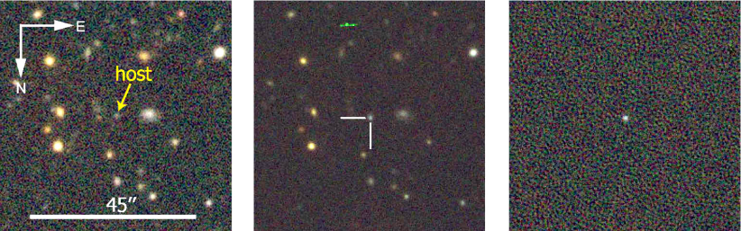
Figure 1: Colour images (riz) of the field surrounding DES13S2cmm. Left: Deep template image created from the co-addition of several epochs of data obtained during the DES Science Verification period in late 2012; the likely host galaxy is indicated by the arrow. Centre: The search image taken close to maximum light (28-Sept-2013) with the position of DES13S2cmm indicated. Right: The difference of the two previous images, clearly identifying DES13S2cmm at center. This image demonstrates the quality of difference images used for discovery and monitoring during the DES observing season.

In Fig. 1 we show DES riz imaging data at the position of DES13S2cmm: pre-explosion, post-explosion, and their difference image. DES13S2cmm is located at $\mathrm{RA}(2000)=02^{\mathrm{h}}42^{\mathrm{m}}32\aas@@fstack{s}82$, $\mathrm{Dec.}~{}(2000)=-01\degr 21\arcmin 30\aas@@fstack{\prime\prime}1$, and was first detected on 2013 August 27 in the DES SN ‘S2’ field (a ‘shallow’ field) located in the Stripe 82 region. DES transient names are formatted following the convention DESYYFFaaaa, where YY are the last two digits of the year in which the observing season began (13), FF is the two character field name (S2), and the final characters (all letters, maximum of 4) provide a running candidate identification, unique within an observing season, as is traditional in SN astronomy (cmm).

3.1 Light Curve

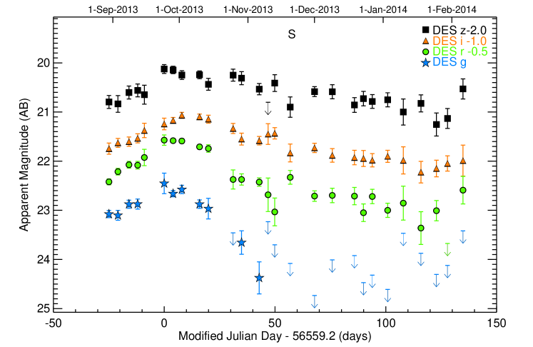
Figure 2: The observed AB magnitude light curve of DES13S2cmm in the four DES SN search filters ($griz$) as a function of the observed phase. ‘S’ denotes the epoch when the ESO VLT spectrum was obtained. The error-bars represent 1-$\sigma$ uncertainties, and the arrow symbols are 3-$\sigma$ upper limits. The phase relative to peak was defined using the observed-frame $r$-band. We have artificially offset (in magnitudes) the $r$, $i$ and $z$ band data for clarity.

In Fig. 2 we present the multi-colour light curve for DES13S2cmm constructed from the first year of DES observations. We have not included upper limits from the earlier, pre-explosion epochs available from the DES SV period in 2012-2013, as these data were taken hundreds of days prior to the data shown in Fig. 2 and are already used to create the reference template image for this field used in the difference imaging detection of the SNe.

We use the photometric pipeline from Sullivan et al. (2011) (also used in Maguire et al., 2012; Ofek et al., 2013) to reduce the DES photometric data for DES13S2cmm. This pipeline is based on difference imaging, subtracting a deep, good seeing, pre-explosion reference image from each frame the SN is present in. The photometry is then measured from the differenced image using a PSF-fitting method, with the PSF determined from nearby field stars in the unsubtracted image. This average PSF is then fit at the position of the SN event, weighting each pixel according to Poisson statistics, yielding a flux, and flux error, for the SN.

We calibrate the flux measurements of DES13S2cmm to a set of tertiary standard stars produced by the DES collaboration (Wyatt et al., in preparation), intended to be in the AB photometric system (Oke & Gunn, 1983). The photometry shown in Fig. 2 has also been checked against the standard DES detection photometry, used to find and classify all candidates for follow-up, and found to be in good agreement. The light-curve data are presented in Table 1.

We correct for Galactic extinction using the maps of Schlafly & Finkbeiner (2011), which estimate ${\rm E(B-V)}=0.028$ at the location of DES13S2cmm, leading to extinction values of 0.123, 0.070, 0.051 and 0.039 magnitudes in the DES $griz$ filters respectively. We do not include these corrections in the values reported in Table 1, but do correct for extinction in all figures and analysis herein, including Figure 2.

Table 1: Light curve data for DES13S2cmm used in Fig. 2. We provide the observed calendar date, modified Julian Day (MJD), observed phase relative to peak MJD (defined relative to peak flux in the r-band), and fluxes (not corrected for Galactic extinction) with 1-$\sigma$ uncertainties in the DES griz passbands. These fluxes can be converted to AB magnitudes using $\mathrm{mag}_{\mathrm{AB}}=-2.5\log_{10}\left(f\right)+31$.

Date	MJD	Phase	$f_{g}$		$f_{r}$		$f_{i}$		$f_{z}$
		(days)
30-AUG-2013	56534.3	-25	1138$\pm$	77	1705$\pm$	94	1730$\pm$	181	1913$\pm$	231
3-SEP-2013	56538.3	-21	1112$\pm$	103	2063$\pm$	129	2234$\pm$	186	1845$\pm$	288
8-SEP-2013	56543.3	-16	1369$\pm$	104	2348$\pm$	148	2285$\pm$	198	2285$\pm$	277
12-SEP-2013	56547.2	-12	1373$\pm$	130	2329$\pm$	167	2433$\pm$	207	2376$\pm$	284
15-SEP-2013	56550.2	-9	$\pm$		2691$\pm$	413	2818$\pm$	380	2193$\pm$	389
24-SEP-2013	56559.2	0	2022$\pm$	388	3727$\pm$	363	3183$\pm$	346	3548$\pm$	295
28-SEP-2013	56563.2	4	1668$\pm$	97	3688$\pm$	133	3400$\pm$	187	3488$\pm$	241
2-OCT-2013	56567.2	8	1805$\pm$	141	3666$\pm$	166	3742$\pm$	209	3169$\pm$	261
10-OCT-2013	56575.2	16	1370$\pm$	108	3285$\pm$	137	3636$\pm$	192	3182$\pm$	230
14-OCT-2013	56579.1	20	1260$\pm$	243	3182$\pm$	223	3482$\pm$	259	2663$\pm$	295
25-OCT-2013	56590.3	31	886$\pm$	346	1782$\pm$	319	2924$\pm$	277	3163$\pm$	352
29-OCT-2013	56594.1	35	667$\pm$	146	1782$\pm$	187	2398$\pm$	267	2987$\pm$	366
6-NOV-2013	56602.1	43	344$\pm$	103	1698$\pm$	132	2326$\pm$	185	2433$\pm$	257
10-NOV-2013	56606.1	47	803$\pm$	426	1338$\pm$	418	2633$\pm$	510	1817$\pm$	634
13-NOV-2013	56609.1	50	-312$\pm$	276	970$\pm$	252	2672$\pm$	281	2726$\pm$	426
20-NOV-2013	56616.1	57	347$\pm$	195	1855$\pm$	239	1848$\pm$	307	1739$\pm$	331
1-DEC-2013	56627.0	68	184$\pm$	107	1306$\pm$	129	2032$\pm$	176	2322$\pm$	216
9-DEC-2013	56635.0	76	259$\pm$	208	1322$\pm$	178	1766$\pm$	225	2318$\pm$	304
19-DEC-2013	56645.1	86	302$\pm$	226	1305$\pm$	211	1697$\pm$	230	1808$\pm$	248
23-DEC-2013	56649.1	90	261$\pm$	136	956$\pm$	157	1667$\pm$	248	2038$\pm$	276
27-DEC-2013	56653.1	94	41$\pm$	156	1295$\pm$	174	1613$\pm$	201	1930$\pm$	248
3-JAN-2014	56660.0	101	252$\pm$	119	1000$\pm$	132	1736$\pm$	196	1993$\pm$	261
10-JAN-2014	56667.1	108	310$\pm$	343	1144$\pm$	364	1609$\pm$	408	1586$\pm$	387
18-JAN-2014	56675.0	116	-75$\pm$	236	717$\pm$	220	1290$\pm$	261	1863$\pm$	297
25-JAN-2014	56682.0	123	306$\pm$	158	992$\pm$	188	1382$\pm$	215	1254$\pm$	270
30-JAN-2014	56687.0	128	345$\pm$	188	523$\pm$	179	1518$\pm$	217	1404$\pm$	261
6-FEB-2014	56694.0	135	-346$\pm$	359	1459$\pm$	376	1602$\pm$	465	2443$\pm$	461

3.2 Spectroscopy

On 2013 November 12, we requested Director’s Discretionary Time at the European Southern Observatory (ESO) Very Large Telescope (VLT) to observe DES13S2cmm, and were awarded target-of-opportunity time within days. The closeness of the object to the moon and instrument scheduling issues conspired to delay observations until 2013 November 21, at which point DES13S2cmm was approximately 30 days after peak brightness (rest frame). A spectrum was obtained with the FOcal Reducer and low dispersion Spectrograph (FORS2 Appenzeller et al., 1998) using the GRIS_300I+11 grism, the OG590 order blocker, and a 1″ slit, with an exposure time of 3600s (3$\times$1200s). This configuration provided an effective wavelength coverage of $5950$ Å to $9400$ Å.

The reduction of the FORS2 data followed standard procedures using the Image Reduction and Analysis Facility environment (v2.16), using the pipeline described in Ellis et al. (2008). This pipeline includes an optimal two-dimensional (2D) sky subtraction technique as outlined in Kelson (2003), subtracting a 2D sky frame constructed from a sub-pixel sampling of the background spectrum and a knowledge of the wavelength distortions determined from 2D arc comparison frames. The extracted 1D spectra were then scaled to the same flux level, the host-galaxy emission lines interpolated over, and the spectra combined using a weighted mean and the uncertainties in the extracted spectra.

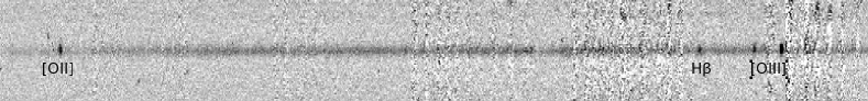
Figure 3: The reduced VLT FORS2 two-dimensional spectrum for DES13S2cmm. The key nebular emission lines used to derive the redshift of the host galaxy, and therefore supernova, are labelled.

In Fig 3 we present our reduced 2D FORS2 spectrum, where wavelength increases to the right along the horizontal axis and the vertical axis is distance along the slit. We highlight the obvious narrow nebular emission lines in the host galaxy of DES13S2cmm, specifically [O ii] $\lambda 3727$ Å, H$\beta$ $\lambda 4861$ Å, and [O iii] $\lambda 4959,5007$ Å. We assume these lines originate from the underlying host galaxy as their spatial extent along the vertical axis is greater than the observed trace of the main supernova spectrum. This observation does not exclude the possibility that such emission lines come from the supernova, but it is difficult to address this issue with our low resolution, and low signal-to-noise, data. We note the observed emission lines are not significantly broadened or asymmetrical, as witnessed in type IIn supernovae.

We see no evidence of any further emission lines, from the SN and/or host galaxy. Therefore, it is unlikely DES13S2cmm is a type II supernova (normal or superluminous).

Using these nebular emission lines, we determine a redshift of $z=0.663\pm 0.001$ for the host galaxy of DES13S2cmm, where the uncertainty is derived from the wavelength dispersion between individual emission lines. This measurement is consistent with the redshift of the SN based on identifications of the broad absorption features seen in the spectrum. As the redshift derived from the host-galaxy spectrum is significantly more precise, henceforth we adopt this value as the redshift to DES13S2cmm.

The spectral classification for DES13S2cmm is based on the superfit program (Howell et al., 2005), which compares observed spectra of SNe to a library of template SN spectra (via $\chi^{2}$ minimisation) while accounting for the possibility of host-galaxy contamination in the data. We added as template spectra of SLSNe-I (PTF09atu, PTF09cnd, PTF10nmn) and SLSN-R (SN 2007bi) to superfit to facilitate our classification. We found that the highest-ranked fits to DES13S2cmm were these SLSNe templates, preferred over templates of normal SN types (e.g., SN Ia). The SLSNe-I templates were slightly better fits to DES13S2cmm than SN 2007bi (SLSN-R), although this may be due to not having a template for SN 2007bi at a similar phase to our spectrum for DES13S2cmm.

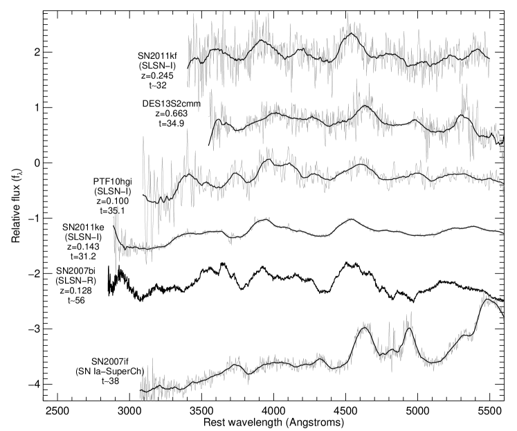
Figure 4: The VLT FORS2 spectrum of DES13S2cmm (second from top) compared to other SLSNe of similar phase in their light curves. From top to bottom, we also show SN 2011kf (Inserra et al., 2013), PTF10hgi (Quimby et al., 2011), SN 2011ke (Inserra et al., 2013) and SN 2007bi(classified as Type R in Gal-Yam et al., 2009); as discussed in Section 3.2, superfit identifies these SLSNe as some of the best-fitting spectral templates to DES13S2cmm. In each case, the light grey shows the raw data and the solid line is a Savitsky-Golay smoothed version of the spectrum. The spectra are labelled with the SN name, SLSN type (except DES13S2cmm), redshift, and the phase when the spectrum was taken. We show the spectrum of the ‘super-Chandrasekhar’ SN Ia SN 2007if as discussed in Scalzo et al. (2010). Note that the spectrum for 2007bi, while at a later phase than the other data, is the earliest spectral observation of this SN.

We show our spectrum of DES13S2cmm in Fig. 4, alongside spectra from other well-studied SLSNe in the literature at a similar phase in their light curves (Quimby et al., 2011; Inserra et al., 2013; Gal-Yam et al., 2009). There is a deficit of spectra for SLSNe in the literature at these late phases for a robust comparison. However, the broad resemblance between the spectra of PTF10hgi, SN 2011kf, SN 2011ke and DES13S2cmm, all taken at approximately $+30$ days past peak, suggests DES13S2cmm is a similar object to these other SLSNe-I. The spectrum of DES13S2cmm is also similar to the spectrum of SN 2007bi (a SLSN-R in Gal-Yam et al., 2009), although the differences between Type I and Type R SLSNe remains unclear, and either classification would be interesting given the sparseness of the data. We also show in Fig. 4 the spectrum of SN 2007if, a ‘super-Chandrasekhar’ SN Ia (Scalzo et al., 2010), an over-luminous ($M_{V}=-20.4$) and likely thermonuclear SN located in a faint host galaxy. This comparison clearly shows that DES13S2cmm is unlikely to be a super-Chandrasekhar SN Ia.

3.3 Host-galaxy properties

The host galaxy of DES13S2cmm is detected in our reference images that contain no SN light. Using sextractor in dual-image mode and the $i$-band image as the detection image, we measure host-galaxy magnitudes of $g=24.24\pm 0.13$, $r=23.65\pm 0.10$, $i=23.31\pm 0.10$ and $z=23.26\pm 0.17$ (AB mag_auto magnitudes). The large photometric errors are due to the relatively shallow depth, and poor seeing, of the template image from the DES SV data – we cannot use the DES first-year data for the host photometry as all epochs of this data contain some light from DES13S2cmm.

The estimated photometric redshift of the host galaxy at the time of discovery was $z_{\mathrm{photo}}=0.86\pm 0.13$ (68 percentile error). This photometric redshift was derived by the DESDM neural network photo-z module code, with uncertainties estimated from the nearest neighbour method, using data taken during SV (Sánchez et al., 2014). Photometric redshifts (when available) are used when selecting SLSN candidates for spectroscopic follow-up, and for DES13S2cmm this redshift implied the event was brighter than $M^{\mathrm{peak}}_{U}=-21$ (typical for SLSNe; Gal-Yam, 2012). Since the start of the first DES observing season the photometric catalog derived from SV data has improved, and presently the DESDM photo-z for the host of DES13S2cmm has improved to $z_{\mathrm{photo}}=0.71\pm 0.06$, which is in better agreement with our measured spectroscopic redshift ($z=0.663\pm 0.001$).

Using the DES host-galaxy photometry and the spectroscopic redshift from VLT, we estimate that the stellar mass of the host galaxy is $\log(M/M_{\odot})=9.3\pm 0.3$ using stellar population models from PEGASE.2 (Fioc & Rocca-Volmerange, 1997), and $\log(M/M_{\odot})=9.0\pm 0.3$ using the stellar population templates from Maraston (2005) (both corrected for Milky Way extinction and fixing the redshift of the templates to $z=0.663$). Such a low stellar-mass host galaxy is consistent with the findings for other SLSNe (Neill et al., 2011; Chen et al., 2013; Lunnan et al., 2014).

We estimate the host-galaxy metallicity from our VLT spectrum using the double-valued metallicity indicator $R_{23}$, defined as $([\textrm{O}\textsc{II}]~{}\lambda 3727+[\textrm{O}\textsc{III}]~{}\lambda\lambda 4959,5007)/H\beta$. Fluxes and uncertainties are derived individually for each emission line from fits of a gaussian plus a first-order polynomial, with the assumption that there is no contamination of the galaxy emission lines from the SN. We compute metallicities using the calibrations of Kobulnicky & Kewley (2004) and McGaugh (1991), and use the formulae derived in Kewley & Ellison (2008) to convert these metallicities into the calibration of Kewley & Dopita (2002) – a step that allows for direct comparison between different methods. We note that since $H\alpha$ and $\textrm{N}\textsc{II}~{}\lambda 6584$ are redshifted to wavelengths beyond our spectral coverage, we cannot determine the branch of the $R_{23}$ function that the metallicity lies on. However, the derived value for $R_{23}$ is close to its theoretical maximum, which minimizes the difference in metallicity estimates between the two branches.

Assuming the lower (upper) branch, we find a metallicity ($12+\log$[O/H]) of 8.30 (8.38) from McGaugh (1991) and 8.30 (8.42) from Kobulnicky & Kewley (2004), which is consistent with the median metallicity of $8.35$ found by Lunnan et al. (2014) for a sample of 31 SLSNe host galaxies. The total uncertainty is dominated by the calibration ($\sim 0.15$ dex), while the statistical uncertainty and the scatter induced by the conversion to Kewley & Dopita (2002) are comparatively negligible. We thus find a host-galaxy abundance ratio that is distinctly sub-solar (8.69; Asplund et al., 2009), though not as extremely low as has been seen for other SLSNe, such as SN2010gx ($12+\log$[O/H]=7.5; Chen et al., 2013).

4 Results

4.1 Bolometric light-curve of DES13S2cmm

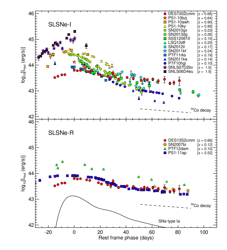
Figure 5: The bolometric light curve of DES13S2cmm (red circles) compared to other SLSNe in the literature (see text for explanation). These bolometric light curves were constructed by fitting a single black-body spectrum to the multicolour data available per epoch (requiring at least three photometric measurements per epoch), and then by integrating the black-body spectral energy distribution to produce the bolometric luminosity per rest-frame epoch (described in detail in Section 4.2). We show statistical errors on the blackbody fits to each epoch of these light curves, but in most cases this error is smaller than the plotting symbol. We stress that these errors do not account for systematic uncertainties involved in the bolometric calculation (e.g., assuming a blackbody for the spectral energy distribution of SLSNe, especially for the UV part of the rest-frame spectral energy distribution). The phase relative to peak (y-axis) for the literature SLSNe is taken directly from the published individual studies and not recalculated herein. The dashed lines shown in both panels represent the expected ⁵⁶Co decay rate at late times. In the lower panel, we show the bolometric light curve expected for a typical Type Ia SNe (solid line) to again illustrate the extraordinary brightness, and extended duration, of these SLSNe

We show in Fig. 5 the bolometric light curve of DES13S2cmm. This single light curve was constructed by fitting a single black-body spectrum to the DES multi-colour data (requiring measurements in a minimum of three photometric bandpasses for a fit), on each epoch in the light curve (Table 1). In detail, we redshift black-body spectra to the observer frame and integrate these spectra through the response functions of the DES filters. We then determine the best-fitting parameters for a black body to the extinction-corrected photometry and integrate this spectrum in the rest frame to obtain the bolometric luminosity per epoch. This procedure benefits from the homogeneity of the DES data as we possess approximately equally-spaced epochs across the whole light curve – typically in four DES passbands – due to our rolling search. The errors on the bolometric luminosities were calculated from the fitting uncertainties on the black-body spectra.

We visually checked our best-fit blackbody curves for each epoch of the DES13S2cmm light curve against the observed $griz$ photometry and found them to be reasonable within the errors. The largest discrepancies were seen in the g-band where some epochs were below the fitted curves, possibly due to UV absorption in the underlying spectral energy distributions relative to a blackbody curve. Inserra et al. (2013) compared the predicted UV flux (from a blackbody curve) for two SLSNe with SWIFT UV observations, and found the fluxes were consistent within the error. Therefore we make no additional correction to the derived bolometric light curve, but note that quantifiable systematic errors in the bolometric luminosity require spectral templates, which in turn requires more spectral data of SLSNe than is currently publicly available.

Using the bolometric light curve of DES13S2cmm, we can determine the peak luminosity of the event and compare it to the definition of a SLSNe in Gal-Yam (2012). This was achieved by integrating the best-fitting black-body spectra through a standard $U$-band filter response function (on the Vega system) to obtain the rest-frame absolute magnitude in $U$-band ($M_{U}$). We find the 2013 September 24 epoch ($t=0$ relative phase in Table 1) gives the largest (peak) absolute $U$-band magnitude of $M^{peak}_{U}=-21.05^{+0.10}_{-0.09}$, which is consistent with the SLSNe threshold of $M^{peak}_{U}<-21$ in Gal-Yam (2012).

We check this result using a model-independent estimate based on the observed $r$-band peak magnitude. At the redshift of DES13S2cmm, the observer-frame $r$ band maps into the rest frame as a synthetic filter with an effective wavelength of $\approx 3800$Å, slightly redward of the standard $U$-band. Defining a synthetic filter as such means the k-correction is independent of the SN spectral energy distribution, and since we are in the AB system the correction is simply $2.5\log(1+z)$. We apply this k-correction to the observed $r$-band peak magnitude, as well as corrections for Galactic extinction and distance modulus, to yield an estimated peak absolute magnitude of $-20.47$ (AB), or $-20.74$ (Vega) in our synthetic filter (where we have computed the AB to Vega conversion for our filter). While this is fainter than our blackbody-based estimate, Vega magnitudes are sensitive to the exact shape of the filter in this region due to the jump in Vega from 3700-3900Å; thus even the small difference in effective wavelength between $U$ band and our synthetic filter can result in significant offsets. The absolute magnitude in our synthetic filter from the best-fitting blackbody method yields $M_{\rm synthetic}=-20.59$, proving that our model-independent estimate is consistent with our results from the blackbody fitting.

We note that the peak magnitude (Vega) for DES13S2cmm classifies it as a SLSN, provided the magnitude is intrinsic to the SN and not enhanced by other effects. Visual inspection of the images in Fig. 1 (including the surrounding areas) shows little evidence for strong gravitational lensing which could affect the observed brightness of this SN (we note that the host galaxy would have to be lensed as well). We cannot conclusively rule out the possibility of strong lensing, as in the case of PS1-10afx (Quimby et al., 2014), but as discussed above the spectrum and extended light curve of DES13S2cmm are inconsistent with a normal SN, while the probability of such a strong lensing event in our DES data is less than the probability of discovering a SLSN, based on the lensing statistics given in Quimby et al. (2014), and the lower redshift of DES13S2cmm and smaller search area of DES. Moreover, the observed $r-i$ peak colour of DES13S2cmm is consistent with the expected colours of other unlensed SNe (including SLSNe) shown in Figure 4 of Quimby et al. (2014), i.e., DES13S2cmm is located below the thick black line in this plot. Therefore, we do not consider gravitational lensing further in this paper, but higher-resolution imaging data should be obtained for DES13S2cmm, after the SN event has vanished, to provide better constraints on possible strong lensing as discussed in Quimby et al. (2014).

4.2 Comparison of bolometric light-curves

For comparison with DES13S2cmm, we also show in Fig. 5 the bolometric light curves for fourteen SLSNe-I (or Ic, as discussed in Inserra et al., 2013) in the literature: PS1-10ky. PS1-10awh (Chomiuk et al., 2011) and PS1-10bzj (Lunnan et al., 2013); SN 2010gx (Pastorello et al., 2010); PTF 10hgi, SN 2011ke, PTF 11rks, SN 2011kf and SN 2012il (Inserra et al., 2013); SNLS 06D4eu and SNLS 07D2bv (Howell et al., 2013); and LSQ 12dlf, SSS 120810 and SN 2013dg (Nicholl et al., 2014). We exclude from this figure, and our analysis, other SLSNe-I that do not possess data for at least three passbands for each epoch (defined as being taken within a 24 hour window) over a majority of their light curves. This criterion, so defined to ensure well-constrained bolometric light-curve fits, excludes namely PTF 09atu, PTF 09cnd, and PTF 09cwl (Quimby et al., 2011); SCP 06F6 (Barbary et al., 2009); and SN 2006oz (Leloudas et al., 2012).

The full bolometric light curves for these SLSNe-I were calculated using the same methodology as described above for DES13S2cmm (i.e. using the published photometric data and requiring three or more passbands per epoch). As a check, our bolometric light curves for PTF 10hgi, SN 2011ke, PTF 11rks, SN 2011kf and SN 2012il are similar to those published in Inserra et al. (2013), with any offsets due to differences in the integration of the blackbody curve; we integrate over all wavelengths, while Inserra et al. (2013) integrate over the wavelength range of their observed optical passbands (we are able to reproduce their luminosities if we follow their procedure). Our bolometric light-curves for PS1-10ky. PS1-10awh, and PS1-10bzj are also similar to those published in the literature.

In Fig. 5, the phase relative to peak for DES13S2cmm was defined as the peak of the observer-frame r-band, which occurred on MJD 56563.2, while for other SLSNe-I we simply used the phase relative to peak as reported by the individual literature studies. In the case of SNLS 06D4eu and SNLS 07D2bv, Howell et al. (2013) reported a phase based on their calculation of the bolometric light curves, which we use herein, but note there may be greater uncertainty in the definition of the time of peak for these light curves.

The top panel of Fig. 5 shows that DES13S2cmm is one of the faintest SLSNe-I around peak compared to the other SLSNe-I in the literature, and possesses one of the slowest declining tails (beyond approximately $+30$ rest-frame) of the SLSNe studied herein. In the bottom panel of Fig. 5, we compare DES13S2cmm to possible Type R SLSNe (to be consistent with the classification scheme of Gal-Yam, 2012) and find the late-time light curve of DES13S2cmm is similar to both PS1-11ap (McCrum et al., 2014) and SN2007bi (Gal-Yam et al., 2009), highlighting the possible overlap between these two SLSNe types, as discussed in Section 3.2 and Inserra et al. (2013).

Fig. 5 also demonstrates that the fifteen SLSNe-I light curves (top panel) have similar luminosities at approximately $+25$ days (rest frame) past peak, close to the inflection point in the light curves when their extended tails begin to appear. We calculate the dispersion, as a function of relative phase, for the SLSNe-I light curves shown in Fig. 5, linearly interpolating between large gaps in each light curve to provide an evenly sampled set of data. We find a minimum dispersion of $\sigma({\rm log_{10}L_{bol}})=0.11$ – equivalent to $0.29$ magnitudes – around $+30$ days past peak (rest frame), derived from the nine SLSNe in Fig. 5 constraining this phase. This dispersion in the light-curves can be decreased to $\sigma({\rm log_{10}L_{bol}})=0.083$, or $0.20$ magnitudes, at approximately $+25$ days past peak (rest frame) if we exclude the four highest redshift SLSNe-I above $z\simeq 1$ (SNLS 06D4eu, SNLS 07D2bv, PS1-10ky. PS1-10awh). The bolometric luminosities of these SLSNe-I are more difficult to estimate because of the uncertainties associated with modelling the UV part of the spectrum by assuming a simply blackbody curve. There could also be evolution in the population with redshift. As commented in Quimby et al. (2011), such light curve characteristics could point towards a possible ‘standardisation’ of SLSNe-I, as with SNe Ia, leading to their use as high-redshift ‘standard candles’ for cosmological studies (King et al., 2014).

Recently, Inserra & Smartt (2014) has proposed a ‘standardisation’ of the peak magnitude of 16 SLSNe using a stretch-luminosity correction similar to the $\Delta m_{15}$ relationship of Phillips (1993) for SNe Ia. They find that SLSNe that are brighter at peak have slower declining light curve over the first $30$ days after peak (rest frame) and, correcting for this correlation, the dispersion of the peak magnitude of SLSNe can be reduced to $\sigma\simeq 0.2$. This is similar in size to the dispersion between $+25$ to $+30$ days past peak seen in Fig. 5 and is only a factor of two worse than the dispersion obtained for standardised SNe Ia.

Both Fig. 5 and Inserra & Smartt (2014) suggest some standardisation of SLSNe light curves is possible but further observations and analyses are required to find the best approach. For example, the light curve of DES13S2cmm does not appear to follow the correlation found by Inserra & Smartt (2014) as it has a faint peak magnitude, relative to other SLSNe, but is also slowly declining towards $+30$ days after peak. A direct comparison to Inserra & Smartt (2014) is difficult as our study uses different sample selection criteria (only 9 of their 16 SLSNe are included here because of our requirement to have three passbands per epoch), while Inserra & Smartt (2014) estimate a common synthetic peak magnitudes for all their SLSNe using their own time-evolving spectral template. A more detailed comparison will be possible with further DES SLSNe.

4.3 Power source of DES13S2cmm

The details of the power source of SLSN-I remain unclear and are much debated (see Section 1). Here we investigate the two popular explanations in the literature for SLSNe-I: radioactive decay of ⁵⁶Ni, and energy deposition from a Magnetar.

4.3.1 Radioactive ⁵⁶Ni model

As can been seen in Fig. 5, the decline rate of DES13S2cmm is approximately that expected from the decay of ⁵⁶Co (dashed line). This is suggestive of the SN energy source being the production and subsequent decay of large quantities of ⁵⁶Ni produced in the explosion. To test this theory we fit the bolometric light curve of DES13S2cmm to a model of ⁵⁶Ni, following the prescription of Arnett (1982), which is the approximation of an homologously expanding ejecta (Chatzopoulos et al., 2009; Inserra et al., 2013) where the luminosity at any given time (in erg s^-1) is given by

$$L(t) =M_{\textrm{Ni}}\,e^{-(t/\tau_{m})^{2}}\biggl{[}\epsilon_{\textrm{Ni}}\int_{0}^{t}\frac{2u}{\tau_{m}^{2}}\,e^{(u/\tau_{m})^{2}}\,e^{-u/\tau_{\textrm{Ni}}}du$$

$$+\epsilon_{Co}\int_{0}^{t}\frac{2u}{\tau_{m}^{2}}\,e^{(u/\tau_{m})^{2}}\biggl{(}e^{-u/\tau_{\textrm{Ni}}}-e^{-u/\tau_{\textrm{Co}}}\biggr{)}du\biggr{]}\delta_{\gamma},$$ (1)

where $u$ is the (time) integration variable. The energy production rate and decay rate for ⁵⁶Ni are $\epsilon_{\textrm{Ni}}=3.9\times 10^{10}$ erg s^-1 g^-1 and $\tau_{\textrm{Ni}}=8.8$ days, while for ⁵⁶Co these values are $\epsilon_{\textrm{Co}}=6.8\times 10^{9}$ erg s^-1 g^-1 and $\tau_{\textrm{Co}}=111.3$ days. The amount of ⁵⁶Ni produced in the explosion is $M_{\textrm{Ni}}$. Parameterizing the rise-time of the light curve, $\tau_{m}$ (from Eqns 18 and 22 of Arnett, 1982) is the geometric mean of the diffusion and expansion timescales, and is given by

$$\tau_{m}=1.05\,\Bigl{(}\frac{\kappa}{\beta c}\Bigr{)}^{1/2}\Bigl{(}\frac{M^{3}_{\textrm{ej}}}{E}\Bigr{)}^{1/4}$$ (2)

Here $E$ is the explosion energy, $M_{\textrm{ej}}$ is the total amount of ejected mass, $\kappa$ is the optical opacity (assumed to be 0.1 cm² g^-1 and constant throughout, as in Inserra et al. (2013)), and $\beta$ is a constant with value $\approx 13.7$ (Arnett, 1982).

We use $\delta_{\gamma}$ to denote the gamma-ray deposition function: the efficiency with which gamma-rays are trapped within the SN ejecta. For this function we follow Arnett (1982), which is also used by Inserra et al. (2013) and uses the deposition function defined in Colgate et al. (1980),

$$\delta_{\gamma}=G[1+2G(1-G)(1-0.75G)],$$ (3)

where $G\equiv\tau_{\gamma}/(\tau_{\gamma}+1.6)$, with the ‘optical depth’ for gamma-rays approximately given by

$$\tau_{\gamma}\approx\Bigl{(}\frac{0.1}{\kappa}\Bigr{)}\Bigl{(}\frac{\tau_{m}^{2}}{4\tau_{\textrm{Ni}}^{2}}\Bigr{)}\Bigl{(}\frac{5.53\times 10^{10}}{v_{ej}(0.1+t/\tau_{\textrm{Ni}})^{2}}\Bigr{)}.$$ (4)

Here $v_{ej}=\sqrt{10E_{k}/3M_{\textrm{ej}}}$ and is in units of cm s^-1. We note that the deposition function used in Chatzopoulos et al. (2009) has a functional form that is similar to that used here, but in their approximation $\tau_{\gamma}$ only deviates from $\approx 1$ at much later epochs, resulting in a light-curve decay rate mirroring ⁵⁶Co and largely insensitive to changes in the explosion energy or ejecta mass.

We thus have four parameters in our model: the explosion epoch ($t_{0}$), the energy of the explosion ($E$), the total ejected mass (M${}_{\textrm{ej}}$), and the amount of ejected mass which is ⁵⁶Ni ($M_{\textrm{Ni}}$). We define the fraction of the ejecta mass that is in ⁵⁶Ni as $f_{\textrm{Ni}}=M_{\textrm{Ni}}/M_{\textrm{ej}}$. We fit our model to the data with a variety of upper limits on $f_{\textrm{Ni}}$, varying from 0.3 to 1.0. However, we follow Inserra et al. (2013) in assuming a physically motivated upper limit on $f_{\textrm{Ni}}$ of 0.5, which they base on the prevalence of intermediate-mass elements in their spectra of lower-$z$ SLSNe, and the calculations of ⁵⁶Ni production in core-collapse SNe by Umeda & Nomoto (2008). We report the best-fitting parameters and goodness of fit for these models in Table 2 as well as show the range of $f_{\textrm{Ni}}$ models in Figure 6 to illustrate the scale of uncertainties in the theoretical modelling.

Table 2: Best-fitting parameters for a variety of ⁵⁶Ni model fits to the bolometric light curve for DES13S2cmm. $f_{\textrm{Ni,max}}$ is the maximum fraction of ⁵⁶Ni allowed in the ejecta for each fit; for DES13S2cmm the best-fitting model always maximizes this value. Ejecta and ⁵⁶Ni masses are given in units of solar masses. There are 22 degrees of freedom for each fit.

$f_{\textrm{Ni,max}}$	$E(10^{51}$ erg)	$M_{\textrm{ej}}$	$M_{\textrm{Ni}}$	$t_{0}$ (MJD)	$\chi^{2}$
0.30	31.88	14.77	4.43	56508.8	81.5
0.40	14.83	10.59	4.23	56510.4	76.0
0.50	8.22	8.21	4.10	56511.5	71.5
0.60	5.08	6.68	4.01	56512.4	67.9
0.70	3.38	5.62	3.93	56513.1	65.0
0.80	2.38	4.84	3.88	56513.7	62.7
0.90	1.74	4.25	3.83	56514.2	60.9
1.00	1.32	3.79	3.79	56514.6	59.4

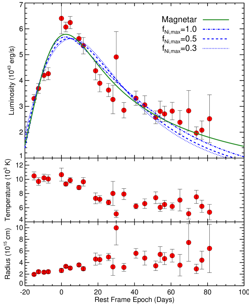
Figure 6: Upper panel: Bolometric light curve of DES13S2cmm, with the best-fit magnetar model (green solid line) and three ⁵⁶Ni models with different $f_{\mathrm{Ni,max}}$ (blue lines) overplotted. The magnetar model is a better match to the data than the best-fit ⁵⁶Ni, and has a significantly better $\chi^{2}$ than the models with a more realistic $f_{\mathrm{Ni,max}}$ (see text). However both models have difficulty reproducing the peak luminosity, the post-peak decline, and the late-time flattening. Middle and Bottom panels: Temperature and radius evolution of the best-fitting blackbody to each photometric epoch which is used to construct the bolometric light curve.

We find that the ⁵⁶Ni model is not a good fit to the bolometric light curve, as the best-fitting model has a $\chi^{2}/\mathrm{dof}=2.7$ ($\chi^{2}$ of 59 for 22 degrees of freedom), and is physically unrealistic ($f_{\textrm{Ni}}=1$). As can be seen in Table 2, the model prediction for $M_{\mathrm{Ni}}$ is relatively robust ($3.8-4.4M_{\odot}$), as this parameter is primarily constrained by the peak luminosity of the light curve. However, to match the late time ($t>30$ days) flattening of the light curve a large amount of ejecta mass or low explosion energy (see Eqn. 2) is required to increase the diffusion time-scale, which simultaneously makes the fit to the post-peak decline poor while predicting a much longer rise time than is seen. We also note that these parameters are poorly constrained individually as $E$ and $M_{\textrm{ej}}$ are correlated (Equation 2), and this degeneracy cannot be broken without the presence of high-quality spectral data (Mazzali et al., 2013).

We do not provide uncertainties on the best fit parameters for each $f_{\textrm{Ni}}$ model in Table 2. This is because the formal uncertainties on parameters (such as $M_{\textrm{Ni}}$) are smaller for each fit than they are between fits with different constraints on $f_{\textrm{Ni}}$. This is due to the simplicity of the ⁵⁶Ni model; we do not consider herein Ni mixing, non-standard density profiles, nor other possible variations in this basic model that could yield different light-curve shapes. For example, it has been noted that a two-component model that is denser in the inner component would produce a quicker flattening post-peak (Maeda et al., 2003).

4.3.2 Magnetar model

As an alternative to the radioactive decay of ⁵⁶Ni, we also fit our derived bolometric light curve for DES13S2cmm to a magnetar model, which proposes that SLSNe are powered by the rapid spinning-down of a neutron star with an extreme magnetic field (Woosley, 2010; Kasen & Bildsten, 2010). In this model the input energy is defined by the initial spin period ($P_{ms}$, in milliseconds) and magnetic field strength ($B_{14}$, in units of $10^{14}$ Gauss) of the magnetar, and the rise-time parameter ($\tau_{m}$, Eqn. 2) reflects the combined effect of the explosion energy ($E$), the ejected mass ($M_{\textrm{ej}}$), and the opacity ($\kappa$). We use the semi-analytical model outlined in Inserra et al. (2013). The luminosity of the magnetar model at time $t$ is given by (in erg s^-1)

$$L(t) =4.9\times 10^{46}\,e^{-(t/\tau_{m})^{2}}\delta\int_{0}^{t}\frac{2u}{\tau_{m}^{2}}\,e^{(u/\tau_{m})^{2}}\,\frac{B_{14}^{2}\,P_{ms}^{-4}}{(1+u/\tau_{p})^{2}}du,$$ (5)

where $u$ is the (time) integration variable, $\tau_{p}$ is the spin-down timescale, $\tau_{p}=4.7\,B_{14}^{-2}\,P_{ms}^{2}$ days, and $\delta$ is the deposition function for the magnetar radiation; here we assume full trapping (i.e., $\delta=1$) following Inserra et al. (2013). We do not include any additional contribution from ⁵⁶Ni decay in this model.

In Fig. 6 we include the best-fitting magnetar model to the bolometric light curve of DES13S2cmm. The best-fitting parameters of this model are a magnetic field of $1.43\times 10^{14}$ Gauss, an initial spin period of $5.28$ ms, a diffusion timescale of $22.9$ days, and an explosion date of MJD 56511.0. This model has a $\chi^{2}/\mathrm{dof}=2.0$ ($\chi^{2}$ of 44 for 22 degrees of freedom) and is therefore a significantly better fit to our data than the ⁵⁶Ni model. However, it is still clear that the model does not fit well: it is unable to reproduce the factor of two drop in luminosity post-peak within 30 days of explosion (although it does a better job than ⁵⁶Ni). Intriguingly the late-time epochs seem to fit the magnetar model well. Our time coverage of DES13S2cmm allows us to determine whether either model is able to reproduce detailed features of the light curve, but discerning between the two models would be improved by an even longer time-scale over which the two models cannot mimic one another; DES alone will unlikely provide longer light curve coverage as its observing season is typically not much more than 5 months a year.

5 Conclusions

In this paper we have presented DES13S2cmm, the first spectroscopically-confirmed superluminous supernova (SLSN) from the Dark Energy Survey. Using spectroscopic data obtained from the ESO Very Large Telescope, we measured a redshift of $z=0.663\pm 0.001$, and assigned a classification of SLSN-I. However, we cannot exclude the possibility that DES13S2cmm is a type R (Fig. 4 and 5) if this is in fact a distinct SLSN type.

Using this redshift and correcting for Milky Way extinction, we find the rest-frame $U$-band absolute magnitude of DES13S2cmm at peak to be $M^{peak}_{U}=-21.05^{+0.10}_{-0.09}$, consistent with the SLSNe definition of Gal-Yam (2012). Like other SLSNe (Lunnan et al., 2014), DES13S2cmm is located in a faint low stellar-mass host galaxy ($\log(\mathrm{M}/\mathrm{M}_{\odot})=8.9\pm 0.3$) with sub-solar metallicity.

In Fig. 5, we compare the bolometric light curve of DES13S12cmm to fourteen similarly well-observed SLSNe-I light curves in literature, and see that DES13S2cmm has one of the slowest declining tails (beyond $+30$ rest frame past peak) of all SLSNe-I studied herein, as well as likely being the faintest at peak. We further find that the dispersion between the bolometric light curves of all SLSNe-I shown in Fig. 5 has a minimum of $0.29$ magnitudes around $+30$ days past peak (rest frame). This reduces to $0.20$ magnitudes around $+25$ days if we remove the four SLSNe-I above $z\simeq 1$ from the measurement because of the increased uncertainty in their rest-frame UV luminosities. This observation raises the tantalising possibility of ‘standardising’ these SLSNe like SNe Ia (Quimby et al., 2011; Inserra & Smartt, 2014) and starting a new era of supernova cosmology (King et al., 2014). Further study is required to confirm if SLSNe can be standardised and investigate further the k-corrections of SLSNe, which would be needed to use SLSNe as robust distance indicators.

In Fig. 6, we fit the bolometric light curve of DES13S2cmm with two possible models for the power source of these extreme events; the radioactive decay of ⁵⁶Ni and a magnetar (e.g. see Inserra et al., 2013). We find that the ⁵⁶Ni model is not a good fit to the bolometric light curve, as the best-fitting model has a $\chi^{2}/$DoF$=2.7$ with an unrealistic fraction of ⁵⁶Ni to ejected mass ($f_{\textrm{Ni}}=1$). The model does provide a relatively robust prediction for the overall ⁵⁶Ni mass ($3.8-4.4M_{\odot}$), as this is primarily constrained by the peak luminosity of the light curve, but is unable to reproduce the late time ($t>30$ days) evolution of the light curve. The Magnetar model provides a smaller $\chi^{2}$ (for the same degrees of freedom) than ⁵⁶Ni, but is likewise not a good fit to the data as it is unable to fully reproduce the drop in luminosity within 30 days of explosion.

In the future, DES should find many more SLSN-I. Such data should allow us to further test these two models, especially if we can measure the (rest frame) light curves to $>100$ days (see Fig. 6 and Inserra et al. 2013). Therefore, we have begun a new project entitled ‘SUrvey with Decam for Superluminous Supernovae’ (SUDSS), which will enable extended monitoring of some DES SN fields (in addition to several non-DES fields) to over 8 months, greatly enhancing both our ability to detect many more SLSNe and measure their long light curves.

Affiliations

¹ Institute of Cosmology and Gravitation, Dennis Sciama Building, University of Portsmouth, Burnaby Road, Portsmouth, PO1 3FX, UK
² School of Physics and Astronomy, University of Southampton, Southampton, SO17 1BJ, UK
³ Berkeley Center for Cosmological Physics, University of California at Berkeley, Berkeley, CA 94720, USA
⁴ Argonne National Laboratory, 9700 S. Cass Avenue, Argonne, IL 60439, USA
⁵ George P. & Cynthia Woods Mitchell Institute for Fundamental Physics & Astronomy, Texas A. & M. University, Dept. of Physics & Astronomy, College Station, TX, USA
⁶ National Center for Supercomputing Applications, 1205 West Clark St., Urbana, IL 61801, USA
⁷Astronomy Department, University of Illinois at Urbana-Champaign, 1002 W. Green Street, Urbana, IL 61801, USA
⁸ Fermi National Accelerator Laboratory, P.O. Box 500, Batavia, IL 60510, USA
⁹Dept. of Physics & Astronomy, University of Pennsylvania 209 South 33rd Street,Philadelphia, PA 19104, USA
¹⁰ Department of Physics, University of Illinois Urbana-Champaign, 1110 W. Green Street, Urbana, IL 61801, USA
¹¹ Astronomy Dept., University of California at Berkeley, Berkeley, CA 94720, USA
¹² Lawrence Berkeley National Laboratory, 1 Cyclotron Road, Berkeley, CA 94720, USA
¹³ Kavli Institute for Cosmological Physics, University of Chicago, Chicago, IL 60637, USA
¹⁴ Department of Physics & Astronomy, 5640 South Ellis Avenue, University of Chicago, Chicago, IL 60637, USA
¹⁵ Australian Astronomical Observatory, PO Box 915, North Ryde NSW 1670, Australia
¹⁶ Cerro Tololo Inter-American Observatory, National Optical Astronomy Observatory, Casilla 603, La Serena, Chile
¹⁷ Department of Physics and Astronomy, University College London, London WC1E 6BT, UK
¹⁸ Space Telescope Science Institute (STScI), 3700 San Martin Drive, Baltimore, MD 21218, USA
¹⁹ Carnegie Observatories, 813 Santa Barbara St., Pasadena, CA 91101, USA
²⁰ Observatório Nacional, Rua Gal. José Cristino 77, Rio de Janeiro, RJ - 20921-400, Brazil
²¹ Laboratório Interinstitucional de e-Astronomia - LIneA, Rua Gal. José Cristino 77, Rio de Janeiro, RJ - 20921-400, Brazil
²² Department of Physics, Ludwig-Maximilians-Universität, Scheinerstr. 1, 81679 München, Germany
²³ Excellence Cluster Universe, Boltzmannstr. 2, 85748 Garching, Germany
²⁴ Jet Propulsion Laboratory, California Institute of Technology,4800 Oak Grove Drive, Pasadena, 91109 CA
²⁵ Department of Physics, University of Michigan, Ann Arbor, MI 48109, USA
²⁶ Department of Astronomy, University of Michigan, Ann Arbor, MI 48109, USA
²⁷ University Observatory Munich, Scheinerstrasse 1, 81679 Munich, Germany
²⁸ Max Planck Institute for Extraterrestrial Physics, Giessenbachstrasse, 85748 Garching, Germany
²⁹ Department of Physics, The Ohio State University, Columbus, OH 43210, USA
³⁰ ICRA, Centro Brasileiro de Pesquisas Físicas, Rua Dr. Xavier Sigaud 150, CEP 22290-180, Rio de Janeiro, RJ, Brazil
³¹ Institut de Física d’Altes Energies, Universitat Autònoma de Barcelona, E-08193 Bellaterra, Barcelona, Spain
³² Institució Catalana de Recerca i Estudis Avançats, E-08010 Barcelona, Spain
³³ Brookhaven National Laboratory, Dept of Physics, Bldg 510A, Upton, NY 11973
³⁴ Department of Physics and Astronomy, Pevensey Building, University of Sussex, Brighton, BN1 9QH, UK
³⁵ SLAC National Accelerator Laboratory, Menlo Park, CA 94025, USA
³⁶ Centro de Investigaciones Energéticas, Medioambientales y Tecnológicas (CIEMAT), Avda. Complutense 40, Madrid, Spain
³⁷ Instituto de Física, UFRGS, Caixa Postal 15051, Porto Alegre, RS - 91501-970, Brazil
³⁸ Kavli Institute. for Particle Astrophysics & Cosmology, Stanford University, Stanford, CA 94305, USA
³⁹ Jodrell Bank Centre for Astrophysics, University of Manchester, Manchester M13 9PL, UK.

References

- Anderson et al. (2014) Anderson L. et al., 2014, MNRAS, 441, 24
- Appenzeller et al. (1998) Appenzeller I. et al., 1998, The Messenger, 94, 1
- Arnett (1982) Arnett W. D., 1982, ApJ, 253, 785
- Asplund et al. (2009) Asplund M., Grevesse N., Sauval A. J., Scott P., 2009, ARA&A, 47, 481
- Barbary et al. (2009) Barbary K. et al., 2009, ApJ, 690, 1358
- Berger et al. (2012) Berger E. et al., 2012, ApJ, 755, L29
- Bernstein et al. (2012) Bernstein J. P. et al., 2012, ApJ, 753, 152
- Bertin & Arnouts (1996) Bertin E., Arnouts S., 1996, A&AS, 117, 393
- Betoule et al. (2014) Betoule M. et al., 2014, arxiv:1401.4064
- Blinnikov & Sorokina (2010) Blinnikov S. I., Sorokina E. I., 2010, arxiv:1009.4353
- Chatzopoulos et al. (2009) Chatzopoulos E., Wheeler J. C., Vinko J., 2009, ApJ, 704, 1251
- Chen et al. (2013) Chen T.-W. et al., 2013, ApJ, 763, L28
- Chomiuk et al. (2011) Chomiuk L. et al., 2011, ApJ, 743, 114
- Colgate et al. (1980) Colgate S. A., Petschek A. G., Kriese J. T., 1980, ApJ, 237, L81
- Cooke et al. (2012) Cooke J. et al., 2012, Nature, 491, 228
- Delubac et al. (2014) Delubac T. et al., 2014, arxiv:1404.1801
- Desai et al. (2012) Desai S. et al., 2012, ApJ, 757, 83
- Diehl & For the Dark Energy Survey Collaboration (2012) Diehl H. T., For the Dark Energy Survey Collaboration, 2012, Physics Procedia, 37, 1332
- Ellis et al. (2008) Ellis R. S. et al., 2008, ApJ, 674, 51
- Fioc & Rocca-Volmerange (1997) Fioc M., Rocca-Volmerange B., 1997, A&A, 326, 950
- Flaugher (2005) Flaugher B., 2005, International Journal of Modern Physics A, 20, 3121
- Flaugher et al. (2012) Flaugher B. L. et al., 2012, in Society of Photo-Optical Instrumentation Engineers (SPIE) Conference Series, Vol. 8446, Society of Photo-Optical Instrumentation Engineers (SPIE) Conference Series
- Gal-Yam (2012) Gal-Yam A., 2012, Science, 337, 927
- Gal-Yam et al. (2009) Gal-Yam A. et al., 2009, Nature, 462, 624
- Howell et al. (2013) Howell D. A. et al., 2013, ApJ, 779, 98
- Howell et al. (2005) Howell D. A. et al., 2005, ApJ, 634, 1190
- Inserra & Smartt (2014) Inserra C., Smartt S. J., 2014, ArXiv e-prints
- Inserra et al. (2013) Inserra C. et al., 2013, ApJ, 770, 128
- Kasen & Bildsten (2010) Kasen D., Bildsten L., 2010, ApJ, 717, 245
- Kelson (2003) Kelson D. D., 2003, PASP, 115, 688
- Kewley & Dopita (2002) Kewley L. J., Dopita M. A., 2002, ApJS, 142, 35
- Kewley & Ellison (2008) Kewley L. J., Ellison S. L., 2008, ApJ, 681, 1183
- King et al. (2014) King A. L., Davis T. M., Denney K. D., Vestergaard M., Watson D., 2014, MNRAS, 441, 3454
- Kobulnicky & Kewley (2004) Kobulnicky H. A., Kewley L. J., 2004, ApJ, 617, 240
- Leloudas et al. (2012) Leloudas G. et al., 2012, A&A, 541, A129
- Lunnan et al. (2014) Lunnan R. et al., 2014, ApJ, 787, 138
- Lunnan et al. (2013) Lunnan R. et al., 2013, ApJ, 771, 97
- Maeda et al. (2003) Maeda K., Mazzali P. A., Deng J., Nomoto K., Yoshii Y., Tomita H., Kobayashi Y., 2003, ApJ, 593, 931
- Maguire et al. (2012) Maguire K. et al., 2012, MNRAS, 426, 2359
- Maraston (2005) Maraston C., 2005, MNRAS, 362, 799
- Mazzali et al. (2013) Mazzali P. A., Walker E. S., Pian E., Tanaka M., Corsi A., Hattori T., Gal-Yam A., 2013, MNRAS, 432, 2463
- McCrum et al. (2014) McCrum M. et al., 2014, arxiv:1402.1631
- McGaugh (1991) McGaugh S. S., 1991, ApJ, 380, 140
- Mohr et al. (2012) Mohr J. J. et al., 2012, in Society of Photo-Optical Instrumentation Engineers (SPIE) Conference Series, Vol. 8451, Society of Photo-Optical Instrumentation Engineers (SPIE) Conference Series
- Neill et al. (2011) Neill J. D. et al., 2011, ApJ, 727, 15
- Nicholl et al. (2014) Nicholl M. et al., 2014, ArXiv e-prints
- Nicholl et al. (2013) Nicholl M. et al., 2013, Nature, 502, 346
- Ofek et al. (2007) Ofek E. O. et al., 2007, ApJ, 659, L13
- Ofek et al. (2013) Ofek E. O. et al., 2013, Nature, 494, 65
- Oke & Gunn (1983) Oke J. B., Gunn J. E., 1983, ApJ, 266, 713
- Pastorello et al. (2010) Pastorello A. et al., 2010, ApJ, 724, L16
- Phillips (1993) Phillips M. M., 1993, ApJ, 413, L105
- Quimby et al. (2011) Quimby R. M. et al., 2011, Nature, 474, 487
- Quimby et al. (2014) Quimby R. M. et al., 2014, Science, 344, 396
- Quimby et al. (2013) Quimby R. M., Yuan F., Akerlof C., Wheeler J. C., 2013, MNRAS, 431, 912
- Riess et al. (1996) Riess A. G., Press W. H., Kirshner R. P., 1996, ApJ, 473, 88
- Sako et al. (2008) Sako M. et al., 2008, AJ, 135, 348
- Sako et al. (2011) Sako M. et al., 2011, ApJ, 738, 162
- Sánchez et al. (2014) Sánchez C. et al., 2014, arxiv:1406.4407
- Scalzo et al. (2010) Scalzo R. A. et al., 2010, ApJ, 713, 1073
- Schlafly & Finkbeiner (2011) Schlafly E. F., Finkbeiner D. P., 2011, ApJ, 737, 103
- Smith et al. (2007) Smith N. et al., 2007, ApJ, 666, 1116
- Sullivan et al. (2011) Sullivan M. et al., 2011, ApJ, 732, 118
- Tripp (1998) Tripp R., 1998, A&A, 331, 815
- Umeda & Nomoto (2008) Umeda H., Nomoto K., 2008, ApJ, 673, 1014
- Woosley (2010) Woosley S. E., 2010, ApJ, 719, L204
- Woosley et al. (2007) Woosley S. E., Blinnikov S., Heger A., 2007, Nature, 450, 390