Simulating biofilm deformation and detachment with the immersed boundary method

Abstract

We apply the immersed boundary (or IB) method to simulate deformation and detachment of a periodic array of wall-bounded biofilm colonies in response to a linear shear flow. The biofilm material is represented as a network of Hookean springs that are placed along the edges of a triangulation of the biofilm region. The interfacial shear stress, lift and drag forces acting on the biofilm colony are computed by using fluid stress jump method developed by Williams, Fauci and Gaver [Disc. Contin. Dyn. Sys. B 11(2):519–540, 2009], with a modified version of their exclusion filter. Our detachment criterion is based on the novel concept of an averaged equivalent continuum stress tensor defined at each IB point in the biofilm which is then used to determine a corresponding von Mises yield stress; wherever this yield stress exceeds a given critical threshold the connections to that node are severed, thereby signalling the onset of a detachment event. In order to capture the deformation and detachment behaviour of a biofilm colony at different stages of growth, we consider a family of four biofilm shapes with varying aspect ratio. Our numerical simulations focus on the behaviour of weak biofilms (with relatively low yield stress threshold) and investigate features of the fluid-structure interaction such as locations of maximum shear and increased drag. The most important conclusion of this work is that the commonly employed detachment strategy in biofilm models based only on interfacial shear stress can lead to incorrect or inaccurate results when applied to the study of shear induced detachment of weak biofilms. Our detachment strategy based on equivalent continuum stresses provides a unified and consistent IB framework that handles both sloughing and erosion modes of biofilm detachment, and is consistent with strategies employed in many other continuum based biofilm models.

74D10, 74F10, 76D05, 76M20.

1 Introduction

The subject of this work is the flow-induced deformation of a biofilm colony, which is a mesoscale collection of bacterial cells held together by an extracellular polymeric network (EPS) that is secreted by the cells. The dimensions of a biofilm colony can be anywhere from tens to hundreds of microns, whereas the size of an individual bacterial cell making up the colony is on the order of 1–5 microns; our focus is on continuum models that treat the biofilm as a viscoelastic solid continuum rather than incorporating the dynamics of individual bacteria. The flow-induced deformations of the biofilm colony affect the fluid dynamic forces acting on it, and thereby also alter both the extent and the mode of detachment (i.e., sloughing or erosion) that may be experienced by the biofilm. We are particularly interested in understanding whether biofilm colonies gain any protection against detachment when they are in close proximity to other colonies. To this end, our aim is to develop a robust numerical method for simulating the interaction between a biofilm colony and the surrounding fluid that is capable of capturing the different modes of biofilm detachment.

Our approach is based on the immersed boundary (or IB) method, in which the biofilm continuum is replaced by a network of Hookean springs. Although the IB method has already been used by several authors for studying biofilm deformation and detachment [1, 26], our approach of computing an equivalent continuum stress at each IB node is markedly different and using it to initiate detachment provides us with a way of handling detachment in a manner that is consistent with other continuum mechanics based models such as [13].

1.1 Bacterial biofilms

Bacterial biofilms are aggregations of microbes that grow on surfaces in an aqueous environment. They form when bacterial cells suspended in the fluid attach themselves to a surface and begin producing an extracellular polymeric substance in which the growing bacteria cells embed themselves. Biofilms play contrasting roles depending on the scenarios in which they are encountered: in waste-water treatment [39] and environmental engineering they play a helpful role; whereas biofilms encountered on medical devices or food-processing equipment can be detrimental in the sense that they cause infections [9] or compromise food safety [48].

In these and other applications, biofilms experience vastly different physical conditions (temperature and pH), hydrodynamics (ranging from creeping to turbulent flow) and chemical environments (rich or sparse in nutrients, or saturated with antibiotics). Their adaptability to diverse conditions is believed to derive at least in part from the mechanical and chemical protection provided by the gel-like EPS layer. It is important from an engineering standpoint to understand the mechanical properties of biofilms so that we can devise effective methods for not only enhancing biofilm growth and survival but also removing them from surfaces. Consequently, over the past 10 years significant effort has been expended to develop novel rheological methods for measuring mechanical properties of biofilms [25]. Such experiments have typically arrived at different conclusions on how to characterize biofilms, with some concluding that they behave as elastic [40] or viscoelastic solids [28], while others liken biofilms to viscoelastic fluids [55]. Furthermore, even within the same material class, measured material parameter values can vary over a fairly wide range. The general consensus is that biofilms behave as (visco-)elastic solids when the applied fluid shear stress is at or near the stresses at which the biofilm was grown, while at higher values of shear stress the biofilm can yield and behave as a viscoelastic fluid. In this paper, we restrict ourselves to the low shear stress case and model the biofilm mechanically as a viscoelastic solid embedded within a viscous fluid.

1.2 Mathematical models of biofilm growth, deformation and detachment

Mathematical models for simulating biofilm growth must take into account a wide range of mechanistic and other dynamical processes, including growth and death of bacteria, attachment of cells to the substratum, transport of solutes (nutrients, metabolic products, antibiotics) within the surrounding fluid and the biofilm itself, reaction kinetics, and removal of bacterial cells as clusters (sloughing) or as individual cells (erosion) when the biofilm EPS matrix weakens in response to fluid shear or chemical treatments. The earliest models developed in the 1980’s [29, 61] assumed that the biofilm is one-dimensional, while many subsequent modelling efforts have attempted to capture the 2D or 3D morphology that develops during biofilm growth processes. The treatment of the hydrodynamics and its interaction with the biofilm has received varying degrees of treatment in these models, ranging from some models that consider biofilm transport processes in isolation and use a specified nutrient concentration boundary layer thickness at the biofilm-fluid interface, whereas other models perform full fluid flow and nutrient transport calculations with or without incorporating fluid-structure interaction effects. A variety of approaches have been developed to model the growth and spreading of the biomass, including individual-based models [32], cellular automata [64], continuum models [2, 13, 30] and phase field models [67]. An exhaustive review of the different modeling approaches can be found in the article [60] and performance benchmark comparisons are available in [14].

Among the more complete models are those that capture multi-dimensional growth and fluid flow [13, 15, 16, 44], although the role played by hydrodynamics in inducing biofilm deformation and detachment has most often received only ad hoc or approximate treatment. These approximations are aimed at capturing the solid mechanics governing the dynamics of the deforming biofilm while simplifying as much as possible the complex fluid flow that surrounds it. The first attempt at solving the solid mechanics problem inside the biofilm and using it to initiate detachment was in [44] where the biofilm was treated as a linearly elastic material and a von Mises yield stress criterion was used to initiate detachment; however, this work neglected the effects of biofilm deformation. In contrast, the particle-based biofilm model in [65] ignored the fluid and proposed a method for initiating detachment using a detachment speed function that is based on the normal velocity of the biofilm-fluid interface. A similar approach has been used in [49], which includes the effects of both biofilm growth and flow by employing a detachment speed that depends on the interfacial shear stress. This approach to initiating detachment rests on the assumption that regions where the interfacial shear stress is highest correspond to locations where the biofilm strain is also high.

One of the aims of the current study is to verify the validity of this last assumption by considering a full fluid-structure interaction simulation that is capable of determining stresses in both fluid and biofilm. We do not explicitly model biofilm growth but rather mimic the effects of growth by considering a family of biofilm colony shapes of different aspect ratio, where each colony size corresponds to a different instant of time during the growth of the same colony. In each case, we investigate how the deformation affects both the mode and the extent of biofilm detachment. This is in contrast with other approaches [13, 44] where the solid mechanics are simulated but any deformations of the biofilm are neglected.

1.3 Fluid-structure interaction in biofilms

During the last several years, significant progress has been made in the study of fluid-structure interaction (FSI) in biofilms, driven by the increased availability of experimental data on biofilm mechanical properties and the motivation to understand the role they play in biofilm survival. Most FSI studies neglect biofilm growth by taking advantage of a natural separation of time scales, in that growth processes are very slow in relation to fluid motion and biofilm deformation. More recently, a phase field method has been applied successfully in 2D [34] and 3D [47] to simulate biofilm growth coupled with deformation arising from interaction with the surrounding flowing fluid treating the biofilm continuum as a multiphase polymeric gel. With the exception of these two works, the most common approach in the biofilm FSI literature combines a Lagrangian discretization of the biofilm with an Arbitrary Lagrangian Eulerian (or ALE) formulation for the fluid. The first study of this kind appeared in [54] where they studied the deformation of a 2D hemispherical biofilm colony placed in a turbulent flow using the ANSYS^® commercial software package. More recently [53], a similar ALE approach was used to study flow-induced oscillations of 2D biofilm streamers and their effect on mass transfer. A more realistic 3D biofilm model was studied in [7] that used sliced 3D confocal laser scanning microscopy data to construct the colony shapes, and employed a nonlinear hyper-elastic constitutive model that accommodates detachment based on a von Mises yield stress criterion.

The aforementioned approaches have the advantage of being well-established in the literature and capable of easily incorporating experimental parameters that measure biofilm rheology. The primary disadvantage is their high computational cost and algorithmic complexity that result from needing to constantly re-mesh the fluid domain as the biofilm colony deforms. Moreover, this re-meshing cost increases enormously if detachment is incorporated in the model.

Motivated by the desire to develop a simpler and more efficient computational approach, Alpkvist and Klapper [1] proposed an alternate FSI strategy based on the immersed boundary (or IB) method in which the biofilm is discretized at a set of moving Lagrangian points. These IB points move relative to an underlying fixed Cartesian grid on which the fluid equations are solved. The elastic properties of the biofilm are captured by distributing forces onto the fluid that derive from a network of Hookean springs joining the IB points. An incompressible fluid pervades both fluid and biofilm regions and the biofilm inherits the density and viscosity of the surrounding fluid, so that the biofilm is actually a visco-elastic composite material consisting of elastic spring forces and fluid viscous forces. This approach has the clear advantage that no re-meshing of the fluid grid is required. To illustrate the versatility of their approach, Alpkvist and Klapper simulated the deformation of both 2D and 3D biofilm structures, while also incorporating a simple detachment criterion based on cutting individual springs when they are stretched beyond a critical length. We remark that other IB models for biofilms were developed prior to [1], namely the work of Dillon and collaborators [11, 10]; however, these authors were concerned with slow flow and the dynamics of individual bacterial cells aggregating and settling on the substratum, and hence the results are relevant to different phenomena occurring on much smaller spatial scales and at much earlier stages of biofilm formation.

A number of other IB approaches have since appeared, such as [57] who performed 3D simulations of biofilm deformation, comparing Hookean (elastic, spring-only) and Kelvin-Voigt (visco-elastic, spring plus dashpot) models for the biofilm material. Using a parametric study of spring stiffness and damping coefficient and comparisons with experiments, they established that realistic biofilm deformation behaviour can be obtained using the IB method. More recently, Hammond et al. [26] developed more detailed 2D and 3D IB models for fragmentation of a biofilm colony in which the location of actual bacterial cells from 3D images was used to determine coordinates of IB points. They employed a similar spring network and detachment strategy as in [1], but they allowed the density of the biofilm to differ from that of the fluid, and in subsequent work [27] also extended their approach to handle variable viscosity.

Despite the increasing popularity of the IB method in biofilm FSI studies, two main challenges remain to be addressed before the method is capable of simulating realistic biofilm deformation and detachment. The first relates to connecting values of the IB spring parameters (elastic stiffness and damping coefficients) to actual biofilm material properties. Despite the parametric study in [57] that showed it was possible to determine suitable parameters for given biofilm colony shape and IB spring network topology, there remains as yet no a priori method for determining IB parameters for a given biofilm.

The second challenge relates to initiating detachment in the IB framework in a way that is consistent with other more established continuum-mechanics-based biofilm studies mentioned in Section 1.2. Whereas IB methods have so far used strain in any given spring as a measure for initiating detachment, this is not a true measure of strain in the continuum mechanics context. Indeed, Hammond et al. [26] demonstrated that when using spring strain as a detachment criterion the resulting biofilm shape is sensitive to the critical strain parameter, and so it is unclear how to choose this parameter to match a given set of biofilm mechanical properties.

1.4 Objectives and outline

In this paper, we aim to address the challenges identified at the end of the preceding section by developing an immersed boundary approach for simulating biofilms that is capable of capturing realistic deformation and detachment behaviours. We begin with a 2D IB model inspired by that of Alpkvist and Klapper [1], and extend this work guided by two main objectives. Our first objective is to develop a novel approach for initiating biofilm detachment that is consistent with methods employed in biofilm models using continuum mechanics based calculations to enact detachment. In this way, we can retain the simpler spring network representation of the biofilm continuum and the advantages it offers, while also implementing a more physically realistic criterion for detachment. Our second major objective is to investigate the effect of flow-induced deformation on both the mechanical stability and mode of detachment experienced by weak biofilm structures having realistic shapes that resemble those grown under mass transfer limited conditions. This will allow us to better understand such fundamental questions as how flow-induced deformation affects the forces acting on biofilms, and how spatial clustering of biofilm colonies can shield them from detachment by reducing the hydrodynamic shear forces.

Our modelling approach incorporates the work done in several previous computational studies of two-dimensional biofilms in [52, 66] wherein we investigated the fluid shear-induced detachment forces (drag and lift) acting on rigid biofilm colonies that are both uniformly and non-uniformly spaced. In contrast to these earlier studies that were restricted to values of shear rate exceeding 10 $\mathrm{cm/s}$, we focus in this paper on more flexible weak biofilm colonies immersed in a slower shear flow having shear rate less than 1 $\mathrm{cm/s}$.

The organization of the remainder of this paper is as follows. In Section 2, we define the problem geometry and parameters, and describe the governing equations and corresponding numerical scheme for our basic IB model framework. Section 3 contains the novel biofilm-related aspects of our IB model where we derive our approach for calculating fluid shear stress along the biofilm-colony fluid interface and from that the drag/lift forces acting on the biofilm colony. In Section 3.1 we describe how we implement a modified version of the exclusion filter devised by Williams et al. in [63] for accurately approximating interfacial shear stresses on curved immersed boundaries, and then in Section 3.2 we describe how we adopt the concept of a continuum stress around each IB node in the biofilm material. Section 3.3 discusses how these quantities are used to obtain a more realistic detachment criterion for biofilm colonies in the IB context. Finally, in Section 4 we perform a number of numerical tests that validate our numerical approach and also demonstrate the advantage of our IB model for simulating realistic deformation and detachment events in fluid shear-induced biofilm dynamics.

2 Immersed boundary (IB) method

The IB method is both a mathematical formulation and a numerical method for simulating the complex interaction between a deformable solid material and a surrounding fluid. The approach dates back to work of Peskin [42] who originally developed the approach to simulate blood flow interacting with heart muscle, and more recent theoretical and computational developments are summarized nicely in the review paper [43]. The IB approach has been applied extensively to the study FSI in bio-fluid mechanics, including such problems as amoeboid locomotion [8], platelet aggregation [19], and sperm motility [18].

The IB method is a mixed Eulerian-Lagrangian approach wherein the fluid equations are discretized on a fixed, rectangular (Eulerian) mesh whereas the elastic structure is defined by a set of (Lagrangian) IB points that move relative to the underlying fluid mesh as the structure deforms. The effect of the immersed boundary on the fluid is represented using a singular source term in the fluid momentum equations, which is distributed onto the underlying fluid grid by writing it as the convolution of an elastic force density with a regularized delta function.

2.1 Problem geometry

A diagram of the problem domain is given in Fig. 1, which depicts shape of a biofilm colony encountered during different stages of growth. The domain is delimited by two horizontal walls separated by a distance $H$, where the bottom wall (serving as the biofilm substrate) is held stationary while the top wall moves horizontally with constant velocity $U_{wall}$. The domain is filled with a viscous, incompressible fluid so that in the absence of biofilm, the top wall will generate a flow that over time approaches a steady-state corresponding to linear (planar) shear with shear rate $G={U_{wall}}/{H}$.

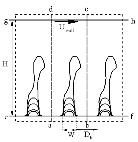
Figure 1: The problem domain consisting of a stationary bottom wall (e-f) separated by a distance $H$ from a top wall (g-h) that moves at velocity $(U_{wall},0)$. Biofilm colonies of width $W_{b}$ and increasing height represent shapes at different stages of growth. The walls are treated with IB points and the whole flow region is embedded in a slightly larger computational domain (abcd) that is periodic in both $x$ and $y$.

Biofilm colonies having identical shape and size are placed along the bottom wall with a uniform spacing of $D_{b}$ between adjacent colonies. In order to simulate biofilms at different growth stages occuring under mass transfer limited conditions, we select four representative biofilm shapes with increasing aspect ratio that have fixed width but increasing height. Motivated by shapes at early stages of growth observed in experiments [12, 31] and 3D simulations [13, 15, 30, 67], we choose an idealized biofilm shape described by the equation

$$\left(\frac{x}{{W_{b}}/{2}}\right)^{n_{1}}+\left(\frac{y}{H_{b}}\right)^{n_{2}}=1\quad\text{with $n_{1},n_{2}>0$ and $y\geqslant 0$},$$ (1)

which is half of a super-ellipse with width $W_{b}$ and height $H_{b}$. In the case when $n_{1}=n_{2}=2$, Eq. (1) reduces to half of a regular ellipse, while further constraining ${W_{b}}=2H_{b}$ yields a semi-circle with radius $H_{b}$.

We believe that this choice is a reasonable parameterization of the typical finger-like shapes that dominate earlier stages of biofilm growth, in contrast with later stages that exhibit a classical mushroom-shaped colony having an ellipsoidal head on top of a thin cylindrical stem. For the purpose of this study, we take values of $n_{1}=n_{2}=2.5$ and $W_{b}=50\;\mathrm{\mbox{$\mu$}m}$, and select a sequence of three initial shapes with $H_{b}=25$, 50 and 75 $\mathrm{\mbox{$\mu$}m}$ respectively. In addition, we consider two other shapes: a semi-circle with diameter 40 $\mathrm{\mbox{$\mu$}m}$ (that is, $n_{1}=n_{2}=2$, $W_{b}=40\;\mathrm{\mbox{$\mu$}m}$ and $H_{b}=20\;\mathrm{\mbox{$\mu$}m}$); and an irregular mushroom-like structure with $W_{b}\approx 60\;\mathrm{\mbox{$\mu$}m}$ and $H_{b}\approx 280\;\mathrm{\mbox{$\mu$}m}$, whose shape is extracted from figures in [1]. The latter mushroom shape is the tallest biofilm colony depicted in Fig. 1 and is chosen to illustrate the effectiveness of the detachment criteria developed in this study by direct comparisons with the results from [1, 26].

Rather than imposing wall boundary conditions directly on the fluid, we simplify the fluid solver by treating the top and bottom walls using immersed boundaries and embed the problem domain inside a slightly larger fluid domain denoted by dashed lines in Fig. 1. Because we are interested in studying repeating arrays of biofilms colonies, periodic boundary conditions are imposed in both the $x$ and $y$ directions so that the computational domain is $\Omega=[0,W]\times[0,H]$ with $W=W_{b}+D_{b}$ (labeled abcd in the figure), and it contains a single biofilm colony.

2.2 Governing equations

The domain $\Omega$ is filled with a Newtonian incompressible fluid having constant density $\rho$ ($\mathrm{g/cm^{3}}$) and dynamic viscosity $\mu$ ($\mathrm{g/cm\;s}$). Denote the infinitesimally thin immersed boundaries representing the fixed bottom wall and moving top wall by $\Gamma_{bot}$ and $\Gamma_{top}$ respectively, and let $\Gamma_{bio}$ represent the solid elastic structure corresponding to the biofilm colony. Note that $\Gamma_{bio}$ is actually a composite material that consists of the elastic force-generating material and fluid that co-exist within the same region. We also assume for the purposes of this study that the biofilm is neutrally buoyant and has the same density as the fluid (although it is straightforward to extend the IB approach to deal with variable density problems [22, 26]). The fluid is therefore governed at all points $\mathbf{x}=(x,y)\in\Omega$ by the incompressible Navier-Stokes equations

$$\rho\frac{\partial\mathbf{u}}{\partial t}+\rho\mathbf{u}\cdot\nabla\mathbf{u}=-\nabla p+\mu\nabla^{2}\mathbf{u}+\mathbf{f},$$ (2)

$$\nabla\cdot\mathbf{u}=0,$$ (3)

where $\mathbf{u}(\mathbf{x},t)$ ($\mathrm{cm/s}$) is the fluid velocity and $p(\mathbf{x},t)$ is pressure ($\mathrm{g/cm\;s^{2}}$).

The effect of the solid boundaries on the fluid is encompassed in the fluid forcing term $\mathbf{f}$, which we consider next. Assume that the configuration of the solid material making up both channel walls and biofilm is described by a function $\mathbf{X}(\mathbf{q},t)$, where $\mathbf{q}$ is a generalized (dimensionless) parameterization that is either a scalar ($\mathbf{q}=s$) in the case of the walls $\Gamma_{bot}$ and $\Gamma_{top}$, or else a vector ($\mathbf{q}=(r,s)$) for a solid region like $\Gamma_{bio}$. The IB force in both cases is specified in terms of a discrete network of IB points connected by springs, and more detail on the precise form of these spring-force connections for walls and biofilm is provided later in Sections 2.4 and 2.5. Assume that the force generated by any deformed configuration can be described by an IB force density function $\mathbf{F}(\mathbf{X}(\mathbf{q},t)$ depending on the current stretched configuration of the spring network. Then the fluid force $\mathbf{f}$ may be determined by spreading the force density at IB points onto the fluid using a delta function convolution

$$\mathbf{f}(\mathbf{x},t)=\int_{\Gamma}\mathbf{F}(\mathbf{X},t)\ \delta(\mathbf{x}-\mathbf{X}(\mathbf{q},t))\;d\mathbf{q},$$ (4)

where $\delta(\mathbf{x})=\delta(x)\delta(y)$ is the Cartesian product of two 1D Dirac delta functions and $\Gamma=\Gamma_{bio}\cup\Gamma_{top}\cup\Gamma_{bot}$ represents the set of all immersed boundaries.

The final equation required to close the system is an evolution equation for the immersed boundaries, which we assume move with the same velocity as the surrounding fluid

$$\frac{\partial\mathbf{X}}{\partial t}=\int_{\Omega}\mathbf{u}(\mathbf{x},t)\delta(\mathbf{x}-\mathbf{X}(\mathbf{q},t)\;d\mathbf{x}.$$ (5)

This is simply another way of stating the no-slip condition for a deformable boundary at location $\mathbf{X}(\mathbf{q},t)$.

2.3 Numerical algorithm

We now describe the basic numerical algorithm for solving Eqs. (2)–(5), which is a semi-implicit scheme very similar to the one employed in [50]. The fluid domain $\Omega$ is discretized on a regular Cartesian mesh with coordinates $\mathbf{x}_{ij}=(x_{i},y_{j})=(ih_{x},jh_{y})$ for $i=0,1,\dots,N_{x}$ and $j=0,1,\dots,N_{y}$, where $h_{x}=W/N_{x}$ and $h_{y}=H/N_{y}$ are constant grid spacings in the $x$ and $y$ directions (and we assume for simplicity that $h_{x}=h_{y}$). The time interval of interest $[0,T]$ is likewise divided into a sequence of $N_{t}$ equally-spaced points denoted $t_{n}=n\Delta t$ for $n=0,1,\ldots,N_{t}$, where $\Delta t=T/N_{t}$ is the time step. Let the discrete values of the velocity and pressure be denoted by $\mathbf{u}_{ij}^{n}$ and $p^{n}_{ij}$ respectively. Suppose that the immersed boundary is described by a set of $N_{b}$ IB points whose locations at any time $t_{n}$ are given by $\mathbf{X}^{n}_{\ell}=(X^{n}_{\ell},Y^{n}_{\ell})$ for $\ell=1,2\ldots,N_{b}$. The corresponding force densities are denoted by $\mathbf{F}^{n}_{\ell}$, with the precise specification of the immersed boundary discretization and force density calculation $\mathbf{F}^{n}_{\ell}$ being given in the the following two sections.

We now describe our algorithm for updating fluid grid quantities $\mathbf{u}^{n}_{ij}$ and $p^{n}_{ij}$ and the IB configuration $\mathbf{X}_{\ell}^{n}$ from time $t_{n}$ to time $t_{n+1}$. The algorithm proceeds in four main steps:

Step 1:

Compute the force density $\mathbf{F}_{\ell}^{n}$ based on the current IB configuration $\mathbf{X}^{n}_{\ell}$ as described in Section 2.5.

Step 2:

Spread the force density onto fluid grid points using a discrete representation of the delta-function convolution in Eq. (4)

$$\mathbf{f}^{n}_{ij}=\sum_{\ell=1}^{N_{b}}\mathbf{F}_{\ell}^{n}\delta_{h}(\mathbf{x}_{ij}-\mathbf{X}^{n}_{\ell}){\cal A},$$ (6)

where $\delta_{h}(\mathbf{x})$ is a regularized delta function given by

$$\delta_{h}(\mathbf{x})=\frac{1}{h_{x}h_{y}}\phi\left(\frac{x}{h_{x}}\right)\phi\left(\frac{y}{h_{y}}\right),$$ (7)

with

$$\phi(r)=\begin{cases}\frac{1}{4}\left(1+\cos(\frac{\pi r}{2})\right),&\text{if }\lvert r\rvert\leqslant 2,\\ 0,&\text{otherwise}.\end{cases}$$ (8)

The scaling factor ${\cal A}$ has units of length for forces generated by the 1D wall interfaces (for which (6) approximates a line integral) whereas ${\cal A}$ has units of area for the 2D biofilm region. To ensure that Eq. (6) is a consistent representation of the corresponding integrals under grid refinement, ${\cal A}$ is inversely proportional to the number of IB points. Details on the precise expression used for ${\cal A}$ in each case are provided in Section 2.5.

Step 3:

Integrate the Navier-Stokes equations using Chorin’s split-step projection scheme:

1. Compute an intermediate velocity $\mathbf{u}^{(1)}_{ij}$ by updating the velocity only for the contribution from the IB elastic force:

   $$\rho\left(\frac{\mathbf{u}^{(1)}_{ij}-\mathbf{u}_{ij}^{n}}{\Delta t}\right)=\mathbf{f}^{n}_{ij}.$$ (9)

2. Compute intermediate velocities $\mathbf{u}^{(2)}_{ij}$ and $\mathbf{u}^{(3)}_{ij}$ by applying convection and diffusion terms using an alternating direction implicit (ADI) approach:

   $$\rho\left(\frac{\mathbf{u}^{(2)}_{ij}-\mathbf{u}^{(1)}_{ij}}{\Delta t}+u^{n}_{ij}D^{0}_{x}\mathbf{u}_{ij}^{(2)}\right)=\mu D^{+}_{x}D^{-}_{x}\mathbf{u}^{(2)}_{ij},$$ (10)

   $$\rho\left(\frac{\mathbf{u}^{(3)}_{ij}-\mathbf{u}^{(2)}_{ij}}{\Delta t}+u^{n}_{ij}D^{0}_{y}\mathbf{u}_{ij}^{(3)}\right)=\mu D^{+}_{x}D^{-}_{x}\mathbf{u}^{(3)}_{ij}.$$ (11)

   The operators $D_{x}^{+}$ and $D_{x}^{-}$ refer to the standard first-order forward and backward difference approximations of the $x$-derivative, and $D_{x}^{0}$ is the standard second-order centered difference approximation. Analogous definitions apply for the $y$-derivative approximations $D^{+}_{y}$, $D^{-}_{y}$ and $D^{0}_{y}$. Equations (10) and (11) thus represent periodic tridiagonal linear systems for the intermediate velocities.

3. Project the intermediate velocity $\mathbf{u}^{(3)}_{ij}$ onto the space of divergence-free vector fields by first solving a Poisson equation for the pressure $p^{n+1}_{ij}$

   $$\nabla_{h}\cdot\nabla_{h}p^{n+1}_{ij}=\frac{\rho}{\Delta t}\nabla_{h}\mathbf{u}^{(3)}_{ij},$$ (12)

   where $\nabla_{h}=(D_{x}^{0},D_{y}^{0})$ is a centered approximation of the gradient operator and the discrete Laplacian $\nabla_{h}\cdot\nabla_{h}$ yields a wide finite difference stencil that spans four grid points in each direction as described in [50]. Because of the periodic boundary conditions, the pressure Poisson equation is solved most efficiently using a fast Fourier transform (FFT). Finally, the velocity projection is completed via the correction

   $$\mathbf{u}_{ij}^{n+1}=\mathbf{u}_{ij}^{(3)}-\frac{\Delta t}{\rho}\nabla_{h}p_{ij}.$$ (13)

Step 4:

Evolve the immersed boundary to time $t_{n+1}$ using

$$\mathbf{X}_{\ell}^{n+1}=\mathbf{X}_{\ell}^{n}+\Delta t\sum_{i,j}\mathbf{u}_{ij}^{n+1}\delta_{h}(\mathbf{x}_{ij}-\mathbf{X}_{\ell}^{n})h_{x}h_{y}.$$ (14)

The IB algorithm explained above is first-order accurate in both time and space. Despite the use of second-order differences for spatial derivatives, the spatial accuracy reduces to first order owing to the particular choice of interpolation used for spreading the fluid velocity onto the immersed boundary [37].

This algorithm has the advantage that it is simple and easy to code, although it suffers from a fairly strict stability restriction on the time step owing to the explicit treatment of the IB forcing term in Step 1 of the algorithm. We implement the above algorithm using MATLAB^®, and when that is combined with the extra cost of implementing a realistic detachment criterion (see details Section 3.3) our approach is restricted to fairly short-time simulations. The scope of this paper is therefore limited to the study of biofilm deformation and detachment in the early stages up until a quasi-steady biofilm configuration in reached. Any full-scale implementation of the detachment criteria described in this study would therefore benefit from a more efficient IB implementation such as the fully implicit approach in [38] or one of the parallel approaches developed in either [24] or [62].

2.4 Discrete representation of walls and biofilm

In this section, we describe the discretization of the immersed boundaries (walls and biofilm) in terms of a network of IB points connected by springs. Section 2.5 will then provide details of the force density calculations based on this discrete IB configuration.

We begin with the horizontal walls at locations $y=0$ and $H$ (labeled e-f and g-h in Fig. 1) that are each replaced by a 1D periodic array of IB points stretching across the domain. Adjacent wall points are not explicitly connected to each other, but instead each IB point is connected by a very stiff spring to a corresponding tether or target point that initially occupies the same position as the IB point. The tether forces generated by these springs constrain the IB points to remain close to their target locations and hence mimic a solid wall. The initial IB point spacing $h_{wall}$ is chosen so that $h_{wall}<\frac{1}{2}\max(h_{x},h_{y})$, which helps to control numerical errors that would otherwise lead to significant leakage of fluid between IB points [43].

Next we consider the discrete representation of the biofilm colony, which is obtained by triangulating the biofilm region, placing IB points at the nodal locations, and constructing a network of Hookean springs corresponding to the edges in the triangulation. The spring stiffness is chosen to approximate the elastic properties of an actual biofilm material. The biofilm is attached to the lower wall by connecting points along the bottom of the colony to a corresponding wall IB point with a stiff spring, where each pair of points initially occupies the same location. To ensure that such a spring network mimics a mechanically isotropic biofilm, we use an initial triangulation that has approximately uniform shape and size of the elements. For this purpose, we use the open-source MATLAB package DistMesh of Persson and Strang [41]. The average spacing between biofilm IB points is initially chosen to be roughly equal to one-third of the fluid grid spacing. This choice is motivated by Vo et al. [57] and ensures that the convective flow inside the biofilm is negligible, so that the biofilm acts as an impermeable material. Nevertheless, we note that during the course of our biofilm simulations as the biofilm deforms and IB points reach their maximum separation, it is possible for portions of the biofilm colony to experience a small apparent permeability. We will return to this point when devising a method for approximating the interfacial shear stress in Section 3.1.

Fig. 2 depicts triangulations of two initial biofilm shapes used in this study, one a super-ellipse with height $H_{b}=75\;\mathrm{\mbox{$\mu$}m}$, and the other a mushroom-shaped biofilm colony with height $H_{b}\approx 280\;\mathrm{\mbox{$\mu$}m}$. A coarser mesh is depicted than what is actually used so that the shape and distribution of triangles are evident.

(a) Super-ellipse shape, with filleted corners at the wall.		(b) Mushroom shape.

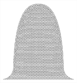
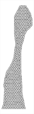
Figure 2: Quasi-uniform triangulations generated by DistMesh for: (a) a super-elliptical biofilm colony with height $H_{b}=75\;\mathrm{\mbox{$\mu$}m}$ and mean edge length 1.5 $\mathrm{\mbox{$\mu$}m}$; and (b) a taller mushroom-shaped colony with mean edge length 4 $\mathrm{\mbox{$\mu$}m}$.

IB simulations with a super-ellipse show that the sharp 90 degree corners at the intersection between the biofilm colony periphery and the bottom wall cause localized discontinuities in the slope of the biofilm colony-fluid interface to develop at these locations as the biofilm colony begins to deform. We believe this is due to the corner-type singularities appearing in the fluid that are communicated to the immersed structure via delta function interpolation. In actual biofilms, such sharp corners seldom occur and so we instead smooth out the corners using a quarter-circular curve or fillet. As depicted in Fig. 2(a), the size of the fillet is kept small so as to minimize its influence on either the biofilm or the corresponding elastic forces.

2.5 Discrete force density calculation

As indicated earlier, the force density function consists of contributions from two classes of immersed boundaries: horizontal rigid walls ($\mathbf{F}_{wall}$) and elastic deformable biofilm regions ($\mathbf{F}_{bio}$). The force contribution in both cases is calculated using a discrete specification that is defined in terms of the current configuration of IB points in either walls or biofilm.

2.5.1 Top and bottom wall forces

The discrete wall force arising at any given wall IB point is determined from the stretched state of the spring of zero resting length that connects it to the corresponding tether point, yielding a force density

$$\mathbf{F}^{n}_{wall,\ell}=\kappa_{wall}\ (\mathbf{X}^{n}_{wall,\ell}-\mathbf{X}^{n}_{teth,\ell}),$$ (15)

where $\kappa_{wall}$ ($\mathrm{g/cm^{2}\;s^{2}}$) is the spring stiffness, and $\mathbf{X}^{n}_{wall,\ell}$ and $\mathbf{X}^{n}_{teth,\ell}$ are the coordinates of the wall at tether points at time level $n$. For the stationary bottom wall all tether points are fixed in time, whereas the top wall tether points move with a given constant velocity $({U}_{wall},0)$ according to

$$\mathbf{X}^{n+1}_{teth,\ell}=\mathbf{X}^{n}_{teth,\ell}+({U}_{wall},0)\Delta t\mod(W,H),$$ (16)

where the “modulo” operator ensures that IB points remain inside the domain by imposing the periodic boundary condition in the horizontal direction. By choosing $\kappa_{wall}$ sufficiently large, we ensure that the wall IB points do not deviate significantly from their tether point locations throughout a simulation. For both sets of wall IB points, we set the integral scaling factor in Eq. (6) equal to the tether point spacing, ${\cal A}=h_{wall}$.

2.5.2 Biofilm forces

The force density at an IB point within the biofilm region is determined by summing up the elastic force contributions coming from all springs connected to that node in the triangulation. Any given spring link is identified by an index pair $\ell,m$ corresponding to two IB points with coordinates $\mathbf{X}_{\ell}^{n}$ and $\mathbf{X}_{m}^{n}$. The elastic force density contribution at node $\ell$ due to spring $\ell,m$ acts in the direction of the vector $\mathbf{d}_{\ell m}^{n}=\mathbf{X}_{\ell}^{n}-\mathbf{X}_{m}^{n}$ joining nodes $\ell$ and $m$. By denoting the resting length of this spring $d^{0}_{\ell m}$, the force density $\mathbf{F}_{bio,\ell}^{n}$ at node $\ell$ owing to all springs attached to that node can be written as [1]

$$\mathbf{F}_{bio,\ell}^{n}=\frac{\kappa_{bio}}{d^{0}}\sum_{m=1}^{N_{b}}\mathbb{I}_{\ell m}\frac{\mathbf{d}_{\ell m}^{n}}{d_{\ell m}^{n}}\frac{(d_{\ell m}^{n}-d^{0}_{\ell m})}{d^{0}_{\ell m}},$$ (17)

where $\kappa_{bio}$ is the spring stiffness coefficient ($\mathrm{g/cm\;s^{2}}$), $d^{0}$ is the average spring resting length and $d_{\ell m}=\|\mathbf{d}_{\ell m}\|$. The symbol $\mathbb{I}_{\ell m}$ is a square connectivity matrix of dimension $N_{b}\times N_{b}$ whose entries are either 1 or 0 depending on whether or not nodes $\ell$ and $m$ are connected. Implicit in this notation is the fact that the summation is only done over pairs of nodes that are connected by an edge in the network. The scaling factor ${\cal A}$ in Eq. (6) for the biofilm force spreading term is taken equal to the average area of a triangle in the biofilm at its rest state, which is equal to the total initial area divided by $N_{b}$ (and hence has units of $\mathrm{cm^{2}}$). Finally, following the arguments of Alpkvist and Klapper [1], we can ensure that the biofilm deformation is independent of grid refinement by scaling the spring stiffness value with the nodal mean distance $d^{0}$ and setting $\widetilde{\kappa}_{bio}=\kappa_{bio}/d^{0}$.

3 Interfacial shear stress, drag and lift forces, and detachment

3.1 Computing forces on the biofilm-fluid interface

Determining the forces acting on a biofilm colony as it deforms in response to fluid shear is of fundamental importance in this study. The most common global measures of hydrodynamic force in such FSI simulations are the drag and lift force. In addition, we are interested in calculating the local interfacial shear stress along the biofilm-fluid interface, owing to its essential role in determining both the mode and extent of biofilm colony detachment. Drag and lift forces are typically calculated in the IB framework by summing the corresponding components of the IB force along the interface [22, 33]. Instead, we follow the approach of Williams, Fauci and Gaver [63] (which we refer from this point on as WFG) wherein the traction force is first calculated from the interfacial shear stress and then integrated along the biofilm-fluid interface. Our aim in this section is therefore to first obtain an expression for interfacial shear stress, and then to derive expressions for the drag and lift forces.

Evaluating interfacial stress in the IB framework is complicated not only by the diffuse nature of immersed boundaries owing to regularized IB forces, but also because of the spatial averaging inherent in the velocity no-slip boundary condition. If not handled appropriately, both of these steps can introduce large errors in interfacial shear stress. This issue was studied by WFG [63] who proposed two methods for calculating the tangential interfacial shear stress based on the equation

$$\underbrace{{\mathbf{t}}\cdot[\boldsymbol{\sigma}]\cdot{\mathbf{n}}}_{\textrm{Jump in FS}}=\underbrace{-\frac{{\mathbf{t}}\cdot\mathbf{F}}{\lvert\frac{\partial\mathbf{X}}{\partial s}\rvert}}_{\textrm{WS}}.$$ (18)

Here, $\mathbf{X}(s,t)$ is a parametric representation of the biofilm-fluid interface, $\mathbf{n}=\frac{\partial\mathbf{X}}{\partial s}/|\frac{\partial\mathbf{X}}{\partial s}|$ is the unit normal vector (directed outward from the biofilm into the surrounding fluid), $\mathbf{t}$ is the counter-clockwise tangent vector, $\boldsymbol{\sigma}=-p\mathbb{1}+\mu(\nabla\mathbf{u}+\nabla\mathbf{u}^{T})$ is the fluid stress tensor, and square brackets $[\cdot]$ denote the jump in a quantity across the interface. WFG proposed evaluating the tangential stress using either side of Eq. (18): the left hand side requires calculating the jump in fluid stress across the biofilm-fluid interface, and so is referred to as the FS method; whereas the right hand side involves local IB force densities, and is called the wall stress or WS method. WFG performed IB simulations of 2D Poiseuille flow in a channel, with and without obstructions, and drew the following conclusions about the relative merits of these two methods:

• On a curved boundary, the WS method over-estimates shear stress in comparison with the FS method.

• In order to maximize accuracy with the FS method, the fluid shear stress associated with an IB point on the interface should be evaluated at a point located inside the domain, directed along the normal vector and separated from the boundary by a distance equal to the fluid grid spacing. The fluid grid cell within which this point falls is called the interpolation box because it defines a set of 4 fluid grid points that will be used for interpolating the stress.

• For a curved immersed boundary, the estimate for shear stress at certain IB points can be adversely affected when the boundary intersects the interpolation box and a portion of the interpolation box lies outside the fluid region. Therefore, only those stresses determined using interpolation boxes that lie entirely on one side of the interface should be included, and for this purpose WFG designed an exclusion filter that omits any such unwanted stress contributions.

We implemented the WFG exclusion filter approach and found that while it works well for the simple immersed boundaries considered in [63], the accuracy of the shear stress calculation degrades for the highly curved interfaces that are so common in biofilm applications. We therefore developed a modified version of the exclusion filter mentioned above that handles highly curved boundaries in a robust fashion.

We begin by explaining the WFG exclusion filter in reference to Fig. 3, which depicts the IB points $\mathbf{X}^{int}_{\ell}$ for $\ell=1,2,\dots,N^{int}$ lying along a biofilm-fluid interface, ordered in the counter-clockwise direction. For each IB point, the outward unit normal $\mathbf{n}_{\ell}$ is computed using a local cubic Lagrange interpolation procedure as explained in [68]. We then identify two points that will be used to evaluate the stress, $\mathbf{XE}^{out}_{\ell}=\mathbf{X}^{int}_{\ell}+h_{x}\mathbf{n}_{\ell}$ and $\mathbf{XE}^{in}_{\ell}=\mathbf{X}^{int}_{\ell}-h_{x}\mathbf{n}_{\ell}$, which lie on either side of the interface located a distance $h_{x}$ along the outward/inward normals from $\mathbf{X}^{int}$, respectively (assuming here that $h_{x}=h_{y}$). The interpolation boxes or fluid grid cells in which these two evaluation points $\mathbf{XE}^{out}_{\ell}$ and $\mathbf{XE}^{in}_{\ell}$ lie are denoted abcd and a$\,{}^{\prime}$b$\,{}^{\prime}$c$\,{}^{\prime}$d$\,{}^{\prime}$, and their respective centroids by $\mathbf{XC}^{out}_{\ell}$ and $\mathbf{XC}^{in}_{\ell}$.

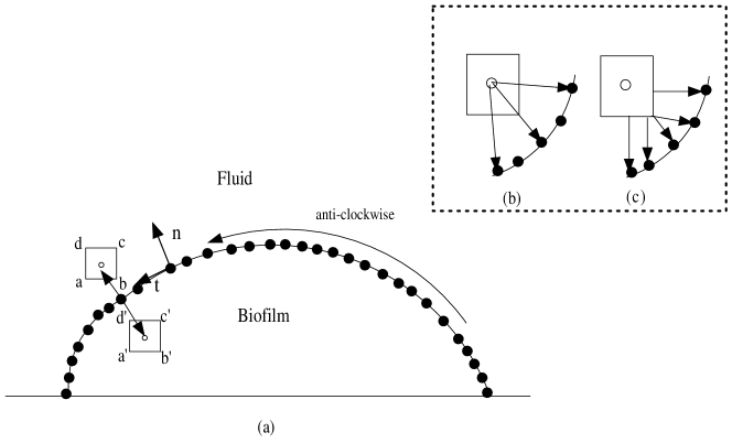
Figure 3: (a) The exclusion filter uses fluid grid cells abcd and a$\,{}^{\prime}$b$\,{}^{\prime}$c$\,{}^{\prime}$d$\,{}^{\prime}$ as the two interpolation boxes, determined by extending an IB point along the outward and inward normals. For the sake of clarity, IB points lying inside the biofilm are not shown here. Distances from the interpolation box to the IB can be calculated in two ways as shown in the inserts: (b) measured from the centroid of the interpolation box, or (c) measured as the shortest distance from the edges.

Then, we calculate the minimum distance from the biofilm-fluid interface to the centroids of the two interpolation boxes (referring to Fig. 3(b)):

$$MD^{out}_{\ell}=\min_{m}\left(D^{out}_{\ell m}\right)\quad\text{and}\quad MD^{in}_{\ell}=\min_{m}\left(D^{in}_{\ell m}\right),$$ (19)

where $m$ ranges over $1,2,\ldots,N^{int}$, and $D^{out}_{\ell m}$ and $D^{in}_{\ell m}$ represent the distance between IB point $m$ and the centroid of the two interpolation boxes associated with the $\ell^{\mathrm{th}}$ IB point.

The main principle behind the WFG exclusion filter [63] is to base stress calculations only on those points that are most representative of the fluid flow around the biofilm colony, first by excluding interpolation boxes that are cut by the interface, and second by choosing stress evaluation points $\mathbf{XE}$ that are as far from the interface as possible (so that they are least affected by the regularized IB force). To this end, we identify IB points $\ell$ for which $MD_{\ell}$ has a local maximum, while also requiring that no interpolation box be used for more than one stress calculation.

As mentioned above, when this WFG filter is applied to biofilms with highly curved interfaces, the accuracy of the stress approximation degrades. One cause of this degradation is that certain portions of the interface may end up with few IB points included, leading to poor resolution. To address this problem, we propose a modification of the WFG exclusion filter that is implemented in Algorithm 1 for stresses on the outer (fluid) side of the interface; only minor changes are required for stresses on the inner (biofilm) side. This new filter makes the following three modifications to the basic WFG exclusion filter:

• In step 8, check whether each interpolation box is cut by the biofilm-fluid interface.

• In step 11, compute the minimum distance between the biofilm-fluid interface and the edges of the interpolation box abcd as shown in Fig. 3(c), rather than the centroid in the original filter. This provides additional resolution by differentiating between nearby IB points that are equidistant from the centroid, since points are not equally-spaced from the edges of the box (compare Figs. 3(b,c)). The minimum distance calculation from the edge of an interpolation box is performed using a fast and elegant algorithm from [4] that introduces no significant additional cost.

• In step 18, the strong local maximum criterion is relaxed and we instead introduce a new user-specified filtering parameter $\epsilon_{min}$. This change ensures (for an appropriate choice of $\epsilon_{min}$) that we retain some IB points that would otherwise have been rejected by the original WFG filter.

Algorithm 1 Modified WFG exclusion filter, which determines a list of IB points (pt_list) and interpolation boxes (box_list) for stress calculations.

1:  for all interface IB points $\mathbf{X}^{int}_{\ell}$ do

2:     Compute the outward unit normal $\mathbf{n}_{\ell}$.

3:     Locate the evaluation point $\mathbf{XE}^{out}_{\ell}=\mathbf{X}^{int}_{\ell}+h_{x}\mathbf{n}_{\ell}$.

4:     Identify the interpolation box abcd corresponding to the fluid cell containing $\mathbf{XE}^{out}_{\ell}$.

5:     Add abcd to the sorted list box_list and remove duplicates.

6:  end for

7:  for all interpolation boxes $\mbox{abcd}\in$ box_list do

8:     if abcd  is intersected by any of the $N^{int}-1$ line segments comprising the biofilm-fluid interface then

9:        Remove abcd from box_list.

10:     else

11:        Determine the minimum distance $MD^{out}_{\ell}$ from the edges of box abcd to the biofilm-fluid interface, and the corresponding IB point $\ell$.

12:        Store $MD^{out}_{\ell}$ and abcd in the data structure for IB point $\ell$.

13:     end if

14:  end for

15:  Initialize pt_list to contain a list of all interface IB points.

16:  for all $\mathbf{X}_{\ell}\in$ pt_list do

17:     Let abcd be the interpolation box corresponding to $\mathbf{X}_{\ell}$.

18:     if either of the neighbouring IB points $\ell\pm 1$ has the same interpolation box abcdor the minimum distance $MD_{\ell}<\epsilon_{min}$ then

19:        Remove $\mathbf{X}_{\ell}$ from pt_list.

20:     end if

21:  end for

After executing Algorithm 1, we obtain a list of IB points at which fluid stress tensor components can be estimated inside corresponding interpolation boxes. We first determine approximations of the velocity derivatives at the corners of each interpolation box using one-sided second-order differences, where the points included in the difference stencils are chosen to lie entirely inside (or outside) the biofilm colony as determined by the unit normal to the interface. We then take the velocity derivatives and pressures, and apply bicubic interpolation [45] to determine corresponding values at the stress evaluation point, which are then combined to obtain the stress tensor components, $\sigma_{11}$, $\sigma_{22}$ and $\sigma_{12}=\sigma_{21}$. In most cases, the set of IB points selected for computing the stress tensor components inside and outside the biofilm colony are different; therefore, computing stress jumps requires that stresses be interpolated onto points in each set. We may then obtain all necessary values of the the stress jump $[\boldsymbol{\sigma}]$ and the tangential component of the interfacial shear stress, $\mathbf{t}\cdot[\boldsymbol{\sigma}]\cdot\mathbf{n}$. Finally, the drag and lift forces are computed by integrating the jump in shear stress along the biofilm-fluid interface using

$$\begin{pmatrix}f_{D}\\ f_{L}\end{pmatrix}=\int\left(n_{1},n_{2}\right)\cdot\begin{pmatrix}[\sigma_{11}]&[\sigma_{12}]\\ [\sigma_{21}]&[\sigma_{22}]\end{pmatrix}\;dS.$$ (20)

3.2 Computing the averaged equivalent continuum stress inside the biofilm

In our IB model, the biofilm continuum is replaced by a network of discrete springs wherein the elastic restoring forces arising from stretched/compressed springs take the place of stress and strain in an real elastic continuum. The most natural way to simulate biofilm detachment within such a spring network representation is to cut any spring links for which the local strain exceeds a critical value, as explained in [1, 27]. However, this approach suffers from several drawbacks. First of all, the force resulting from stretching or contraction of a 1D spring element cannot accurately capture the actual strain in an elastic continuum and consequently there is no direct way to determine a critical spring strain threshold based on measured biofilm mechanical properties. This contrasts markedly with other approaches such as [7, 13, 44] that discretize the solid mechanics equations directly and employ a more physically realistic von Mises yield stress criterion to initiate detachment. In addition, there is no reliable way in the spring network approach to determine spring parameters so as to ensure that different triangulations exhibit similar detachment dynamics under the same flow conditions.

In order to bridge this gap between continuum mechanics-based biofilm models and the discrete IB spring-based model, we introduce the notion of a stress tensor defined at each node in the network. This is accomplished by assuming that there is an equivalent continuum representative elementary area or REA surrounding each node, within which we compute an average value of the stress tensor components in terms of the spring forces acting on that node. The primary motivation for this definition comes from the Discrete Element Method (DEM) for computing microstructural stress in a granular medium [5, 20]. In the DEM, the dynamics of a granular medium are determined by treating each grain separately and solving the governing force balance equations under the combined action of grain contact forces, body forces and external forces. In place of grains we have IB points, and our Hookean spring connections replace the contact forces between the grains.

3.2.1 Constructing the REA around each IB point

In contrast with DEM simulations of granular media that identify an REA with a Voronoi cell constructed from a Delaunay triangulation [5], we employ instead a control volume finite element method construction [59] that is based on a (non-Delaunay) triangulation generated by DistMesh [41]. For each biofilm point labelled $I$ in the triangulation, the corresponding REA is constructed by joining with straight lines the centroids of all surrounding triangles to the mid-points of the corresponding edges (springs) emanating from node $I$ as depicted in Fig. 4. If there are $m$ springs connected to node $I$, then the corresponding REA is a polygon with $2m$ sides. By this construction, we note that the area $A$ of the REA around a node (which is required for calculating the stress tensor later in Eq. (29)) is one-third of the total area of all triangles surrounding the node. This REA construction extends in a straightforward manner to volumes in three dimensions.

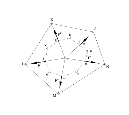
Figure 4: The representative elementary area (REA) surrounding IB node $I$ corresponds to the polygonal region ${\cal P}$ (shown using dashed lines) connecting the centroids ($a,b,c,d,e$) of the surrounding triangles to mid-points ($j,k,l,m,n$) of the edges emanating from node $I$.

3.2.2 Computing the equivalent continuum stress tensor

Consider the REA surrounding a point $\mathbf{X}^{I}$ in the triangulation, pictured as a dashed polygonal region in Fig. 4. Denote the REA and its boundary by ${\cal P}$ and $\partial{\cal P}$ respectively, and let $A$ refer to the area of ${\cal P}$. Suppose that an equivalent continuum material occupies the REA, with stress field having Cartesian components $\sigma^{eq}_{ij}$ for $i,j=1,2$. Then the average stress over ${\cal P}$ is

$$\overline{\sigma}_{ij}^{eq}=\frac{1}{A}\iint_{\cal P}\sigma^{eq}_{ij}\;dA,$$ (21)

which can be manipulated to obtain

$$\overline{\sigma}_{ij}^{eq}=\frac{1}{A}\iint_{\cal P}\sigma^{eq}_{kj}x_{i,k}\;dA=\frac{1}{A}\iint_{\cal P}\left[(\sigma^{eq}_{kj}\ x_{i})_{,k}-x_{i}\ \sigma^{eq}_{kj,k}\right]\;dA,$$

where the subscript “$,\,k$” denotes a $k$-component derivative and the Einstein summation convention is assumed for repeated indices. The divergence theorem may then be applied to the first term to get

$$\overline{\sigma}_{ij}^{eq}=\frac{1}{A}\left(\oint_{\partial{\cal P}}\sigma^{eq}_{kj}x_{i}n_{k}\;dS-\iint_{\cal P}x_{i}\ \sigma^{eq}_{kj,k}\;dA\right).$$ (22)

Now consider the two types of force that can act on the REA: a surface traction force $T_{j}(\mathbf{x})$ that acts at points on the REA boundary, and a body force $g_{j}(\mathbf{x})$ acting at interior points. Imposing a force balance on the boundary yields

$$\sigma^{eq}_{ij}n_{i}(\mathbf{x})=T_{j}(\mathbf{x})$$ (23)

at points $\mathbf{x}\in\partial{\cal P}$, where $n_{i}$ denotes the outward-pointing unit normal vector to $\partial{\cal P}$. We note here that the convention in solid mechanics is to use the inward normal (which ensures compressive stresses are positive), however we break this convention for the sake of consistency with rest of the text. Balancing forces in the interior of the REA gives

$$\sigma^{eq}_{ij,i}\;\;+\;\;\rho g_{j}=\rho a_{j},$$ (24)

where $a_{j}$ is the $j$–component of acceleration. Substituting Eqs. (23)–(24) into (22) then yields

$$\overline{\sigma}_{ij}^{eq}=\frac{1}{A}\left(\oint_{\partial{\cal P}}x_{i}T_{j}\;dS\;\;+\;\;\iint_{\cal P}\rho x_{i}(g_{j}-a_{j})\;dA\right).$$ (25)

We now introduce notation for IB nodes $\mathbf{X}^{\alpha}$, $\alpha=J,K,L,M,N$, that are immediate neighbors of node $I$ in the triangulation shown in Fig. 4, along with corresponding edge vectors $\mathbf{E}^{\beta}$ for $\beta=j,k,l,m,n$ directed outward along springs (with $\mathbf{E}^{j}=\mathbf{X}^{J}-\mathbf{X}^{I}$ when $\beta=j$, for example). The edge mid-points are then denoted by $\mathbf{Z}^{\beta}=\mathbf{X}^{I}+\mathbf{E}^{\beta}/2$, with corresponding spring forces $\mathbf{F}^{\beta}$. If we associate the boundary traction force $\mathbf{T}(\mathbf{x})$ for $\mathbf{x}\in\partial{\cal P}$ with the spring forces $\mathbf{F}^{\beta}$, then the boundary integral term in (25) may be rewritten in component form as

$$\oint_{\partial{\cal P}}x_{i}T_{j}\;dS=\sum_{\beta\in\partial{\cal P}}Z^{\beta}_{i}F^{\beta}_{j}.$$ (26)

Substituting this expression into (25) yields

$$\overline{\sigma}_{ij}^{eq} =\frac{1}{A}\left(\sum_{\beta\in\partial{\cal P}}Z^{\beta}_{i}F^{\beta}_{j}+\iint_{\cal P}\rho x_{i}(g_{j}-a_{j})\;dA\right).$$ (27)

We assume in this paper that the biofilm is neutrally buoyant and that the equivalent continuum stress is computed in a steady-state configuration for which inertial forces are negligible; consequently, the integral term in Eq. (27) is zero. The remaining summation term can be further simplified by substituting $\mathbf{Z}^{\beta}=\mathbf{X}^{I}+\mathbf{E}^{\beta}/2$ and using the equilibrium condition

$$X^{I}_{i}\sum_{\beta\in\partial{\cal P}}F^{\beta}_{j}=0,$$ (28)

to obtain

$$\left(\overline{\sigma}_{ij}^{eq}\right)_{I}=\frac{1}{2A}\sum_{\beta\in\partial{\cal P}}E^{\beta}_{i}F^{\beta}_{j}.$$ (29)

We note that this averaged equivalent continuum stress tensor is guaranteed to be symmetric ($\overline{\sigma}_{ij}^{eq}=\overline{\sigma}_{ji}^{eq}$), which should be contrasted with the analogous derivation for granular media where the DEM approach leads to a non-symmetric stress tensor owing to contact forces with a nonzero moment about grain centers [5]. This does not happen in our IB spring network because elastic spring forces always act along lines connecting IB points and hence do not generate any such moments.

For our choice of polygonal REA around node $I$, the area $A$ in (29) is equal to one-third of the total area of all triangles surrounding the node. If we apply our stress calculation method to a biofilm that only deforms and experiences no detachment, the number of springs connected to each node is constant and a simple data structure can be used to store the information needed to compute stress. Furthermore, the area $A$ and edge vector components ${E}_{i}^{\beta}$ are easily updated using the current IB node coordinates. However, in the more complicated case with detachment, extra geometric information must be stored along with the IB point data; for example, we must keep track of the changing number springs connecting each IB node as well as the number of active triangles around each node. The necessary changes to the code and data structures are straightforward, and the added computational cost is negligible in comparison to that for the IB algorithm.

3.3 Biofilm detachment criterion

As mentioned earlier, we handle biofilm detachment using a yield stress criterion from the von Mises stress theory, which is one of many approaches used to model failure of a ductile material subjected to external loading [3]. The von Mises yield stress criterion has been employed successfully in the context of biofilm modeling [7, 13, 44], even though the biofilm composite (composed of cells, EPS and fluid) is not strictly a ductile material. In two dimensions, the von Mises yield stress at any IB point inside the biofilm region can be expressed in terms of the averaged equivalent continuum stress tensor components in Eq. (29) as

$$(\sigma_{von})^{2}=(\overline{\sigma}^{eq}_{11})^{2}-\overline{\sigma}^{eq}_{11}\overline{\sigma}^{eq}_{22}+(\overline{\sigma}^{eq}_{22})^{2}+3(\overline{\sigma}^{eq}_{12})^{2}.$$ (30)

The value of $\sigma_{von}$ is then compared to some threshold yield stress, which is a measure of the biofilm cohesive strength. If $\sigma_{von}$ exceeds the threshold, then detachment is initiated by severing all springs connecting it to neighbouring IB points. This should be contrasted with other approaches based on edge strain [1, 27], wherein springs are cut individually based on some threshold strain value and an IB point is only detached from the colony when all springs connected to it are severed.

The detachment process in the case of biofilms is complicated somewhat by the fact that yield strength varies throughout the biofilm colony. For example, the strength with which the base of the biofilm colony adheres to the substratum, which we call the biofilm adhesive strength $\Sigma_{adh}$, is several orders of magnitude larger than the cohesive strength of the bulk biofilm material. Furthermore, the bulk cohesive strength also varies since the portion of the colony nearest the biofilm-fluid interface has a stress threshold $\Sigma_{coh}^{ext}$ that is significantly smaller than the value $\Sigma_{coh}^{int}$ in the interior. Consequently, we have three threshold values satisfying $\Sigma_{coh}^{ext}<\Sigma_{coh}^{int}<\Sigma_{adh}$, which leads to a natural separation of the biofilm into three zones – substratum, interface and interior.

With this in mind, we propose the following detachment strategy. First, for any given IB point $\mathbf{X}_{\ell}$ we calculate the shortest distance from point $\ell$ to the substratum and to the biofilm-fluid interface, denoted by $D_{\ell}^{sub}$ and $D_{\ell}^{ext}$ respectively. We then select a yield stress criterion to be imposed by determining which zone the IB point belongs to:

Zone 1:

consists of all IB points near the substratum that satisfy $D_{\ell}^{sub}\leqslant\epsilon^{sub}$, where $\epsilon^{sub}$ is a user-specified parameter. In this case, the point detaches whenever $\sigma_{von}\geqslant\Sigma_{adh}$.

Zone 2:

consists of any of remaining IB points near the biofilm-fluid interface that satisfy $D_{\ell}^{ext}\leqslant\epsilon^{ext}$. Here, the point detaches when $\sigma_{von}\geqslant\Sigma_{coh}^{ext}$.

Zone 3:

consists of all remaining interior biofilm points, which detach if $\sigma_{von}\geqslant\Sigma_{coh}^{int}$.

Calculating the distance $D_{\ell}^{sub}$ is trivial because the bottom wall in our numerical simulations is parallel to the $x$–axis. However, the calculation of $D_{\ell}^{ext}$ is more involved owing to the irregular biofilm shape and also because the colony deforms in time, hence requiring that $D_{\ell}^{ext}$ be recalculated in each time step. Therefore, care must be taken in order to design an efficient algorithm for estimating $D_{\ell}^{ext}$; for this purpose we employ a finite element-based signed distance function for triangles developed in [17], which is an extension of the fast marching method. The cost of this algorithm can be optimized by only calculating the distance function at IB points lying within a narrow band near the interface. As an illustration, Fig. 5 shows sample contour plots of $D_{\ell}^{ext}$ for two different biofilm colony shapes.

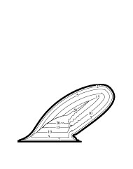
Figure 5: Contours of the distance function $D_{\ell}^{ext}$ (labels in $\mathrm{cm}$) from any given IB point to the biofilm-fluid interface, computed using the algorithm in [17]. Two biofilm colonies are shown near steady-state: (a) the elliptical configuration Sup75, and (b) a mushroom-shaped colony.

The treatment of biofilm detachment is performed after completing Step 1 (the force calculation step) in the immersed boundary algorithm. The steps in the yield stress based detachment process are summarized in Algorithm 2. We note that in the implementation outlined here, we make use of three integer arrays of “status flags” – named *_STATUS with * = INODE, ISPRING, ITRI – one each for IB nodes, springs and triangles. These flags are set to either 0 or 1 depending on whether the status is detached or active, respectively.

Algorithm 2 Biofilm detachment algorithm based on equivalent continuum stress and the von Mises yield stress criterion.

1:  For each IB node $\ell$, compute the distance from the substratum, $D_{\ell}^{sub}$.

2:  Identify IB nodes $\ell$ that lie on the interface, and assign $D_{\ell}^{ext}=0$ there.

3:  At all remaining IB nodes, compute the distance function $D_{\ell}^{ext}$ using the algorithm in [17].

4:  for all IB nodes $\mathbf{X}_{\ell}$ that are active (with INODE_STATUS = 1) do

5:     Compute the REA area $A$ as the sum of areas of all active triangles (with ITRI_STATUS = 1) neighbouring node $\ell$.

6:     Use all active springs (with ISPRING_STATUS = 1) to calculate the equivalent continuum stress components $\sigma^{eq}_{ij}$ from Eq. (29).

7:     Compute the von Mises yield stress $\sigma_{von}$ using Eq. (30).

8:     if $D_{\ell}^{sub}\leqslant\epsilon^{sub}$ then

9:        Let THRESHOLD = $\Sigma_{adh}$.

10:     else if $D_{\ell}^{ext}\leqslant\epsilon^{ext}$ then

11:        Let THRESHOLD = $\Sigma_{coh}^{ext}$.

12:     else

13:        Let THRESHOLD = $\Sigma_{coh}^{int}$.

14:     end if

15:     if $\sigma_{von}\geqslant$ THRESHOLD then

16:        Let INODE_STATUS = 0 (detached).

17:        For each spring adjacent to this node, set ISPRING_STATUS = 0.

18:        Use INODE_STATUS and ISPRING_STATUS to update the status of the triangle associated with the detached node to inactive (ITRI_STATUS = 0).

19:     end if

20:  end for

4 Numerical simulations

4.1 Model parameters

Table 1 summarizes all parameter values used in our numerical simulations of biofilm–fluid interaction. The parameters are separated naturally into the following categories:

Table 1: Parameter values for the various numerical test cases.

Description		Values
Fluid domain:
	Domain height	$H=3\times H_{b}$
	Colony spacing	$D_{b}=50,\ 150,\ 250,\ 400\;\mathrm{\mbox{$\mu$}m}\;(W_{b},3W_{b},5W_{b},8W_{b})$
Biofilm shape (width and height):
	Semi-circle:	$W_{b}=40\;\mathrm{\mbox{$\mu$}m}$, $H_{b}=20\;\mathrm{\mbox{$\mu$}m}$ (Semi20)
	Super-ellipse:	$W_{b}=50\;\mathrm{\mbox{$\mu$}m}$, $H_{b}=25\;\mathrm{\mbox{$\mu$}m}$ (Sup25)
		$W_{b}=50\;\mathrm{\mbox{$\mu$}m}$, $H_{b}=50\;\mathrm{\mbox{$\mu$}m}$ (Sup50)
		$W_{b}=50\;\mathrm{\mbox{$\mu$}m}$, $H_{b}=75\;\mathrm{\mbox{$\mu$}m}$ (Sup75)
Fluid/biofilm grid:
	Fluid grid spacings	$h_{x}=h_{y}=0.5\;\mathrm{\mbox{$\mu$}m}$ (Semi20, Sup25)
		$h_{x}=h_{y}=0.75\;\mathrm{\mbox{$\mu$}m}$ (Sup50, Sup75)
	IB wall point spacing	$h_{wall}=\frac{1}{4}\min(h_{x},\;h_{y})$
	Biofilm spring rest-length	$d^{0}=0.15\;\mathrm{\mbox{$\mu$}m}$ (Semi20, Sup25)
		$d^{0}=0.225\;\mathrm{\mbox{$\mu$}m}$ (Sup50, Sup75)
Fluid/biofilm material properties:
	Fluid density	$\rho=1.0\;\mathrm{g/cm^{3}}$
	Fluid viscosity	$\mu=0.01\;\mathrm{g/cm\;s}$
	Shear rate	$G=0.625\;\mathrm{s^{-1}}$
	Biofilm spring stiffness	$\kappa_{bio}=0.75d^{0},\;7.5d^{0},\;75d^{0}\;\;\mathrm{g/cm^{2}\;s^{2}}$
	Wall spring stiffness	$\kappa_{wall}=10^{5}\;\mathrm{g/cm^{2}\;s^{2}}$

• Biofilm geometry: We took four different biofilm colony shapes, one a semi-circle of radius $20\;\mathrm{\mbox{$\mu$}m}$ and width $W_{b}=40$ (labeled Semi20), and three (semi-)super-ellipses having width $W_{b}=50\;\mathrm{\mbox{$\mu$}m}$ and height $H_{b}=25$, $50$ and $75\;\mathrm{\mbox{$\mu$}m}$ (labeled Sup25, Sup50, Sup75 respectively). These dimensions are representative of typical biofilm colonies and also capture a range of aspect ratios observed in early stages of biofilm colony growth.

• Fluid domain: The vertical spacing $H$ between top and bottom channel walls is set to triple the height of the biofilm colony ($H=3H_{b}$) in order to minimize boundary effects. Simulations reveal that at our results are relatively insensitive to changes in $H$. The width of the fluid domain is $W_{b}+D_{b}$, and values of $D_{b}=W_{b}$, $3W_{b}$, $5W_{b}$ and $8W_{b}$ were used to study the effect of colony spacing.

• Fluid grid: We chose relatively small values of fluid grid spacing $h_{x}$ and $h_{y}$ that permit accurate resolution of the biofilm colony. In particular, we aimed to ensure that recirculating eddies arising from flow separation are well captured. A constant time step of $\Delta t=10^{-5}\;\mathrm{s}$ was used in all simulations.

• Biofilm grid: The mean spacing $d^{0}$ between biofilm IB points was chosen to satisfy $d^{0}\leqslant\frac{1}{3}\min(h_{x},\;h_{y})$ as in [57] so as to avoid numerical errors due to leakage of fluid between IB points. This value of $d^{0}$ is provided to the DistMesh code as a measure of average edge length for the biofilm triangulation; for example, the Sup75 biofilm colony with $d^{0}=0.225\;\mathrm{\mbox{$\mu$}m}$ yields a triangulation with 81,449 IB nodes and $222,659$ edges.

• Fluid material properties: We take fluid parameters consistent with water: $\rho=1\;\mathrm{g/cm^{3}}$ and $\mu=0.01\;\mathrm{g/cm\;s}$. The shear rate was set to $G=0.625\;\mathrm{s^{-1}}$ for all simulations, which is high enough to induce large deformations in weak biofilm colonies while also attaining a steady state over a relatively short time period (roughly 2–8 $\mathrm{s}$). This shear rate corresponds to a Reynolds number $Re={\rho GW_{b}^{2}}/{\mu}=1.5625\times 10^{-3}$ for the case $W_{b}=50\;\mathrm{\mbox{$\mu$}m}$, where we have used the width of the biofilm colony as a length scale.

• Biofilm material properties: To mimic weak biofilms with varying mechanical strength, we choose several values of the IB spring stiffness corresponding to $\widetilde{\kappa}_{bio}=0.75$, 7.5 and 75, where we recall that $\widetilde{\kappa}_{bio}={\kappa_{bio}}/{d^{0}}$. The wall spring stiffness $\kappa_{wall}=10^{5}$ is chosen much larger so that wall points do not move appreciably.

In summary, we consider four different biofilm shapes, four colony spacings and three values of the spring constant, corresponding to a total of 48 simulations with a single value of shear rate $G=0.625\;\mathrm{s^{-1}}$.

4.2 Model validation: Channel with a rigid bump

Before applying our immersed boundary algorithm to the biofilm test cases outlined in the previous section, we first validate our numerical approach using a simpler set-up consisting of a rectangular channel containing a rigid semi-circular bump on the bottom wall. The same problem was considered in Williams et al. [63] as an illustration of their exclusion filter approach for interfacial stress calculation.

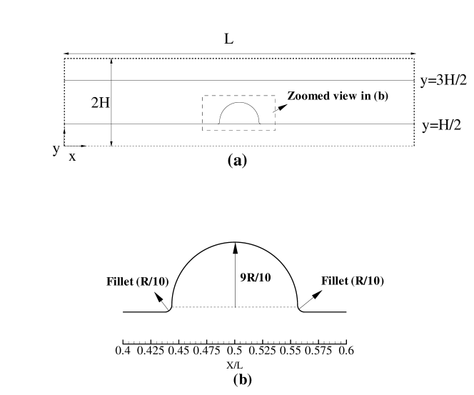
Figure 6: (a) Computational domain for the channel flow with a rigid bump. The fluid domain is a box of size $L\times 2H$ containing two parallel, horizontal walls at height $y=\frac{H}{2}$ and $\frac{3H}{2}$. Attached to the bottom wall is a filleted (smoothed) semi-circular bump. The flow is driven from left to right through the central channel by imposing a constant (positive) fluid body force. (b) Zoomed view of the semi-circular obstruction.

The problem geometry is shown in Fig. 6, consisting of a channel of width $H$ constructed from two parallel horizontal walls along $y=\frac{H}{2}$ and $y=\frac{3H}{2}$. The channel is embedded within a larger rectangular fluid domain of size $L\times 2H$ and periodic boundary conditions are imposed the outer boundaries. A constant fluid body force $\mathbf{f}_{B}(\mathbf{x})=(\Delta P/L,\;0)$ is applied at each fluid grid point inside the channel, which in the absence of any obstruction would generate a parabolic Poiseuille flow with pressure difference $\Delta P$ across the channel from left to right. However, an obstruction is introduced within the channel consisting of an immersed boundary in the shape of a semi-circle of radius $\frac{9R}{10}$ and centered at $(\frac{L}{2},\;\frac{H}{2}+\frac{R}{10})$. The corners connecting the bump to the bottom wall are smoothed using quarter-circular fillets with radius $\frac{R}{10}$ as shown in Fig. 6(b) that serve to regularize the IB shape and avoid flow irregularities near sharp corners.

The channel walls and semi-circular obstruction are represented using IB points, each of which is connected by a single spring to a tether point that is fixed in space, and the spring stiffness is chosen large enough that the IB points do not move appreciably. The spacing $h_{wall}$ between adjacent IB points is chosen so that $h_{wall}\leqslant\frac{1}{2}\min(h_{x},\;h_{y})$, which aims to minimize any numerical errors arising from leakage of fluid across the immersed boundaries.

We choose parameter values the same as in [63], namely $H=0.1\;\mathrm{m}$, $L=0.8\;\mathrm{m}$, $R=0.05\;\mathrm{m}$, $\Delta P/L=-10^{5}\;\mathrm{kg/m^{2}}$, $\mu=25\;\mathrm{kg/m\;s}$, $\rho=1\;\mathrm{kg/m^{3}}$ and $\kappa=10^{9}\;\mathrm{kg/m^{2}\;s^{2}}$. In contrast with the CGS units used in the rest of this paper, we employ MKS units in this section only for ease of comparison with the results in [63]. The fluid domain is discretized on a uniform grid of $512\times 128$ points and we use a constant time step $\Delta t={0.16\rho h_{wall}^{2}}/{\mu}$. The Reynolds number based on channel height is $Re={\rho\Delta PH^{3}}/({8\mu^{2}L})\approx 0.02$, which indicates that inertial effects are negligible and permits us to make comparisons with the Stokes flow solution from Gaver and Kute [21].

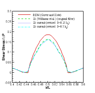
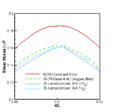
Figure 7: (a) Dimensionless interfacial shear stress computed along a semi-circular obstruction in a channel. For comparison, results are included from another IB approach [63] and the boundary element method [21]. (b) Close-up view near the apex of the bump where shear stress attains a maximum.

The computed interfacial shear stress, non-dimensionalized by $\Delta P$, is shown in Fig. 7(a) along the central portion of the bottom wall including the semi-circular bump. Results are presented for two values of the exclusion filter parameter, $\epsilon_{min}=0.15h_{x}$ and $0.4h_{x}$. Also included in this figure are numerical results computed with two other methods, namely the WFG method with an FS-based exclusion filter [63], and the boundary element computations of Gaver and Kute [21]. The results from our revised exclusion filter are within approximately 5% of WFG’s results, with the differences most pronounced on either side of the crest of the bump (see Fig. 7(b)). The correspondence with WFG’s results improves as $\epsilon_{min}$ increases from $0.15h_{x}$ to $0.4h_{x}$, which can be explained as follows: even though the number of IB points retained by the filter decreases with increasing $\epsilon_{min}$, the quality of those points is high because they are separated further from the smearing effects of the interface.

A non-dimensional flow rate can be computed by integrating the computed velocity vertically along the channel inlet

$$Q=\frac{12\mu L}{H^{3}\Delta P}\int_{y=\frac{1}{2}H}^{y=\frac{3}{2}H}u(0,y)\;dy,$$ (31)

yielding a value of $Q=0.554$ that agrees exactly with the result of WFG [63] for the same grid resolution. We also compute the dimensionless drag

$$f^{\ast}_{D}=\frac{L}{RH\Delta P}\int_{\Gamma}T_{1}\;dS,$$ (32)

where $T_{1}$ is the $x$–component of the traction force and $\Gamma$ represents the portion of the bottom wall corresponding to the semi-circular bump. Our simulations yield $f^{\ast}_{D}=4.662$ and $5.195$ for filter parameters $\epsilon_{min}=0.15h_{x}$ and $0.40h_{x}$ respectively, which should be compared with the WFG result of 5.617. This discrepancy of 7–17% is acceptable in view of the increased flexibility we gain from our modified filter in terms of being able to compute stress along strongly-curved biofilm interfaces.

4.3 Simulating biofilm deformation: Flow structure and forces

In this section, we investigate the response of deformable biofilm colonies to a shear flow by studying the effect of changes in various parameters on the biofilm shape, flow structure, hydrodynamic drag and interfacial shear stress.

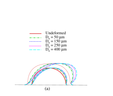
Figure 8: Initial (undeformed) and steady-state (deformed) biofilm shapes with $\widetilde{\kappa}_{bio}=0.75$ as the spacing between colonies $D_{b}$ is varied. (a) Test cases Semi20 and Sup25. (b) Test cases Sup50 and Sup75.

We begin by varying the inter-colony spacing $D_{b}$ for the four initial colony shapes Semi20, Sup25, Sup50, Sup75. Fig. 8 depicts the initial and final (steady-state) biofilm profiles for values of $D_{b}$ lying between 50 and $400\;\mathrm{\mbox{$\mu$}m}$, holding the stiffness parameter $\widetilde{\kappa}_{bio}=0.75$. The extent of the deformation clearly increases as the biofilm height is increased, with the largest deformations occurring for the Sup75 colony. This behaviour is physically reasonable because longer structures are not only more flexible but also extend further into the shear flow where they experience a higher flow velocity. The extent of deformation also increases with the spacing parameter $D_{b}$, which is to be expected since the shear flow is more able to impinge between colonies having a greater separation.

Note that our simulated biofilm colonies appear to simply shear to the right without exhibiting any of the elongation or vertical lifting that is observed in the numerical simulations of Vo et al. [57, 58]. This discrepancy can be attributed to several sources: (a) Vo et al. used different colony shapes having a sinusoidal profile that is much taller (corresponding to $H=180\;\mathrm{\mbox{$\mu$}m}$); (b) their spring stiffness is roughly 100 times larger than ours; and (c) they also considered a much faster flow corresponding to $Re=230$ (based on hydraulic diameter of the square capillary reactor as length scale) whereas we have $Re={\rho GW_{b}^{2}}/{\mu}\approx 10^{-3}$ (based on a much shorter length scale $W_{b}$ corresponding to the biofilm width). It was also suggested in [58] that a significant contributor to elongation from lifting at high enough Reynolds number is inertial effects arising from biofilm deformation as well as the nature of the flow surrounding the colony.

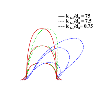
Figure 9: Final (steady state) biofilm shapes for different values of $\widetilde{\kappa}_{bio}$ and constant colony spacing $D_{b}=250\;\mathrm{\mbox{$\mu$}m}$. The super-ellipse test cases Sup25, Sup50 and Sup75 are shown.

We next investigate the effect of changes in the spring stiffness on the steady-state deformation, taking values of $\widetilde{\kappa}_{bio}=0.75$, 7.5 and 75 for three different initial colony shapes while holding $D_{b}=250\;\mathrm{\mbox{$\mu$}m}$ constant. Fig. 9 depicts the final deformed shapes from which we observe that at the lowest shear rate, even a relatively modest value of biofilm stiffness $\widetilde{\kappa}_{bio}\approx 7.5$ is sufficient to resist deformation. Indeed, it is only when stiffness is reduced to $\widetilde{\kappa}_{bio}=0.75$ that any significant bending of the biofilm colony occurs.

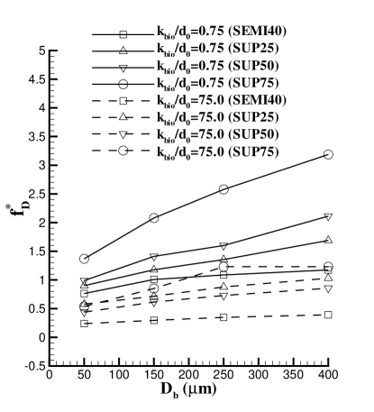
Figure 10: Variation of dimensionless drag force $f^{\ast}_{D}$ (at steady state) with colony spacing $D_{b}$. Curves are shown for four different initial colony shapes and for $\widetilde{\kappa}_{bio}=0.75$, $75$.

The drag force acting on the biofilm at steady state is then computed for all of simulations above. Fig. 10 plots the drag force in each case as a function of colony spacing $D_{b}$. Here, the drag force has been non-dimensionalized using $f^{\ast}_{D}=f_{D}/(\mu GW_{b})$, where the reference value $\mu GW_{b}$ can be thought of as the force exerted by a linear shear flow with shear rate $G$ acting on a very thin biofilm colony with $H_{b}\ll W_{b}$. The corresponding lift force is not shown because lift is much smaller than drag (by at least a factor of 10), not to mention that lift force is much less affected by changes in colony spacing. We observe from Fig. 10 that $f^{\ast}_{D}$ is an increasing function of $D_{b}$, with the rate of increase being largest for the weakest biofilms having $\widetilde{\kappa}_{bio}=0.75$. In particular, as $D_{b}$ increases from 50 to 400 $\mathrm{\mbox{$\mu$}m}$, the drag force increases by a factor of 50% for cases Sup25 and Sup50, with the largest colony in Sup75 exhibiting a roughly 100% increase in drag. These results should be contrasted with the simulations of rigid biofilms in [52] where the drag force was non-monotonic, attaining a local minimum at some intermediate value of $D_{b}$. Because the drag fails to level out at the upper end of the range $W_{b}\leqslant D_{b}\leqslant 8W_{b}$ considered here, we would have to explore significantly larger values of colony separation in order to obtain results consistent with an isolated biofilm colony. Because a much larger domain size would be required, we have not investigated this high-$D_{b}$ regime for reasons of high computational cost.

Another observation is that for stiffer biofilms ($\widetilde{\kappa}_{bio}=7.5$ and 75) organized into the closest-spaced colonies ($D_{b}=50\;\mathrm{\mbox{$\mu$}m}$), the drag force increases by at most 20% as the colony height increases from Semi20 to Sup75, whereas the drag on the weaker biofilms ($\widetilde{\kappa}_{bio}=0.75$) increases by more than 50%. This should be contrasted with the widest-spaced colonies ($D_{b}=400\;\mathrm{\mbox{$\mu$}m}$) where the drag increase for stiff biofilms is roughly 100% and over 150% for weak biofilms. In the latter case, the majority of the drag increase occurs when the biofilm height increases from 50 to 75 $\mathrm{\mbox{$\mu$}m}$, which cannot be accounted for by the increase in colony surface area alone (i.e., perimeter in 2D). We therefore conclude that biofilm colonies may be able to grow into tall structures even if they are weak mechanically because of the protection they gain from having other colonies in close spatial proximity.

More insight into the causes and extent of fluid-induced deformation can be derived by visualizing the flow structure using path-lines or fluid particle trajectories. Fig. 11 depicts four path-line plots for the Sup75 case, corresponding to biofilms that are weak/stiff (with $\widetilde{\kappa}_{bio}=0.75$, 75) and spaced closely/widely ($D_{b}=50$, 400). For the stiffer biofilm, the flow over the widest-spaced colony in Fig. 11(d) clearly exhibits flow separation both upstream and downstream of the colony. As the spacing between the stiff biofilm colonies is reduced, the up/downstream eddies merge to form a single large eddy as pictured in Fig. 11(c), which is similar to what has been observed in numerical simulations of rigid biofilms at high shear rates [52, 66].

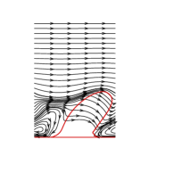
(a) $D_{b}=50\;\mathrm{\mbox{$\mu$}m}$, $\widetilde{\kappa}_{bio}=0.75$

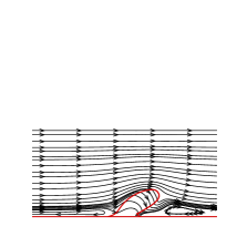
(b) $D_{b}=400\;\mathrm{\mbox{$\mu$}m}$, $\widetilde{\kappa}_{bio}=0.75$

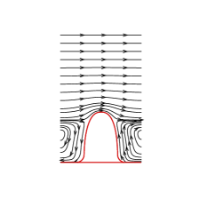
(c) $D_{b}=50\;\mathrm{\mbox{$\mu$}m}$, $\widetilde{\kappa}_{bio}=75$

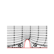
(d) $D_{b}=400\;\mathrm{\mbox{$\mu$}m}$, $\widetilde{\kappa}_{bio}=75$

Figure 11: Pathlines for Sup75 showing the flow structure and biofilm deformation as a function of stiffness and colony separation.

In the case of a weak biofilm, the eddy structure and dynamics are more interesting. In narrow-spaced colonies ($D_{b}=50$) the deflection of the weak biofilm causes the single eddy located between the neighbouring colonies to become distorted and “climb” the upstream face as seen in Fig. 11(a). For more widely-spaced colonies ($D_{b}=400$) with two distinct eddies present, the increased deformation in the weak biofilm causes the upstream eddy to shrink while the downstream eddy grows, as shown in Fig. 11(b).

We remark that for the weak biofilms in Figs. 11(a,b), path-lines clearly traverse the interior of the colony which corresponds to a very slow flow (slower by several orders of magnitude than the flow outside the biofilm region). The spring network making up our simulated biofilm therefore behaves like a porous medium, which has a very small permeability [51] that can be attributed to small volume conservation errors that are well-studied in the context of the IB method [23]. The porous flow is so small that it has minimal effect on the biofilm deformation or the flow, but it cannot be ignored when computing shear stress along the interface using the FS method described earlier in Section 3.1. The porosity is particularly important along portions of the biofilm–fluid interface that experience flow separation adjacent to recirculating eddies on the upstream and downstream faces of the colony. The effect of the weak porous flow inside the biofilm colony is accounted for in the FS method by including its contribution to the jump term in Eq. 18. This requires performing the filtering operation twice: once to select IB points suitable for calculating the fluid stress component outside the biofilm colony, and second time for the stress inside. As mentioned earlier in Section 3.1, different IB points are selected for the stress calculations inside and outside the biofilm colony, necessitating an interpolation between the two sets of IB points. This is in contrast with the stress calculations of WFG [63], where the interior flow was assumed to be weak and its contribution to the interfacial stress was neglected. This assumption did not affect their calculated interfacial shear stress, since there was no flow separation at the low Reynolds numbers they considered.

To conclude this section, we investigate the interfacial shear stress distribution along the biofilm-fluid interface, which is depicted in Fig. 12 for weak/stiff biofilms ($\widetilde{\kappa}_{bio}=0.75$, 75) that are closely/widely spaced ($D_{b}=50$ and $400\;\mathrm{\mbox{$\mu$}m}$).

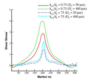
(a) Case Semi20

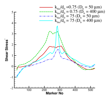
(b) Case Sup25

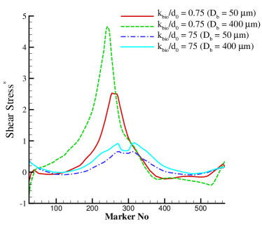
(c) Case Sup50

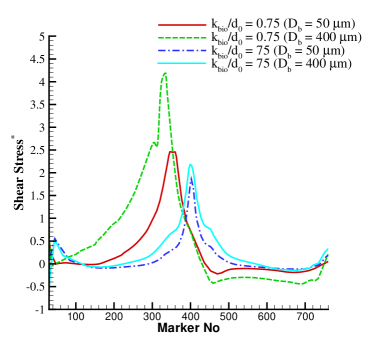
(d) Case Sup75

Figure 12: Dimensionless interfacial shear stress plotted as a function of IB point index, numbered from left to right along the biofilm-fluid interface. Results are shown for cases Semi20, Sup25, Sup50 and Sup75, with two values of colony spacing ($D_{b}=50$, $400\;\mathrm{\mbox{$\mu$}m}$) and two stiffness values ($\widetilde{\kappa}_{bio}=0.75$, 75).

The shear stress is plotted against the IB point index numbered from left to right along the interface (note that the total number of IB points increases with the size of the colony). In all cases, the shear stress is non-dimensionalized using the reference value $\mu G$, which corresponds to the steady uniform shear flow that would occur in the absence of any obstacle. We adopt a sign convention that assumes stress is positive when the flow adjacent to the biofilm-fluid interface is in the same direction as the primary channel flow (i.e., from left to right). A zero shear stress indicates a point where flow separates and a recirculating eddy attaches to the biofilm surface.

For each test case depicted in Figs. 12(a)–(d) there are four curves, which can be separated into two pairs having similar shape: one pair corresponding to weak biofilms with high shear stress, and the second to stiff biofilms with low shear stress. Within each pair of curves, increasing the colony spacing from 50 to 400 $\mathrm{\mbox{$\mu$}m}$ causes the maximum shear stress to increase but leaves the general shape of the stress curve unchanged; however, there is a slight downstream shift of the location of the maximum stress for the three super-ellipse cases SupNN.

In summary, these results indicate that both the magnitude of the shear stress and its variation along the interface can change significantly when the biofilm colony deforms. We will see next that this has important implications for biofilm detachment.

4.4 Simulating biofilm detachment using equivalent continuum stress

To demonstrate the effectiveness of our equivalent continuum stress-based detachment strategy, we now consider a different colony shape pictured in Fig. 1. This mushroom-shaped colony features wide head and base sections connected by a relatively narrow stem. The reason for using this shape is two-fold: first, these long and thin structures are more realistic especially during the advanced stages of deformation just before a detachment event; and second, that it allows comparison with other IB studies of biofilm deformation and detachment that use similar mushroom shapes [1, 27]. Based on solid mechanics principles and experimental evidence, we know that when such an elongated colony is subjected to a sufficiently strong shear flow, it will rupture at a location inside the narrow stem region where the cross-sectional area is smallest. Consequently, this scenario serves as a simple validation of our detachment algorithm.

The precise mushroom shape used in our simulations is extracted digitally from [1, Fig. 3a] which in turn was taken from experimental images. We use the following values of the physical and geometric parameters: $H=300\;\mathrm{\mbox{$\mu$}m}$, $D_{b}=240\;\mathrm{\mbox{$\mu$}m}$, $h_{x}=h_{y}=5\;\mathrm{\mbox{$\mu$}m}$, $d^{0}=1.25\;\mathrm{\mbox{$\mu$}m}$, $G=0.625\;\mathrm{s^{-1}}$ and $\widetilde{\kappa}_{bio}=15$. As before, DistMesh is used to triangulate the initial biofilm region, yielding a total of 6155 IB nodes connected by 6500 edges (springs). In the remainder of this section, we present results using two different detachment strategies: the first based on spring strain; and the second based on equivalent averaged continuum stress. In particular, we aim to identify the drawbacks of the strain-based approach that in turn highlight the advantages of our new equivalent averaged continuum stress approach developed in Section 3.

4.4.1 Spring strain-based detachment

We start by considering a detachment strategy based on spring strain, $\varepsilon_{\ell m}=d_{\ell m}/d^{0}_{\ell m}-1$, where $d_{\ell m}$ represents the length of a spring and $d^{0}_{\ell m}$ is the corresponding unstressed (or resting) length. The central parameter in this detachment model is the critical strain, $\varepsilon_{max}$, beyond which the spring will break. Other studies employing a similar detachment criterion [1, 27] have used $\varepsilon_{max}\equiv 1$, which coincides with detachment occuring when a spring is stretched to twice its resting length. The reason for this choice of critical strain was not justified, even though it is evident on physical grounds that $\varepsilon_{max}$ should not be constant but rather depend on the strength of the biofilm matrix (which in our IB model is expressed by $\widetilde{\kappa}_{bio}$).

As an illustration of strain-based detachment, we simulate flow over the mushroom-shaped biofilm using the parameters indicated above. Fig. 13 depicts the resulting biofilm configuration at four equally-spaced times between $t=0$ and $1\;s$. Unlike the SupNN (super-ellipse shaped) test cases, we have not simulated the mushroom shaped colony for long enough time to reach a quasi-steady state. Up to time $t=1\;\mathrm{s}$, the mushroom shaped colony exhibits continuous deformation characterized by a near-constant IB point displacement velocity of approximately 60$\;\mathrm{{\mathrm{\mbox{$\mu$}m}}/{s}}$ (not shown in the figure). Fig. 13 shows the edges in the deformed triangulation after 0.75 seconds, colored according to the local strain value. For the sake of clarity, we have only shown the edges with strain greater than 0.1 (where positive strain corresponds to a spring that is stretched relative to the resting configuration). Clearly, the base of the colony near the substratum experiences the highest strain, with values near 0.5. The next highest edge strains (between 0.25 and 0.5) occur in sizable portions of the head and base as well as a few points near the midsection of the stem region, which can be seen in the zoomed view in Fig. 13. An alternate view of the stem is shown in Fig. 14, with the edges having negative strain colored green, while edges with strain greater than 0.25 are colored magenta (and all other edges shown in black). The high strain (magenta) edges are clearly aligned along the long axis of the colony, whereas those experiencing compression (negative strain, green) are aligned at an angle of 45–60 degrees to the main colony axis.

We now illustrate a critical drawback of the spring strain-based detachment methodology that has not received attention in earlier biofilm IB studies [1, 27]. We assume that detachment is initiated after 0.75 s of deformation and apply a critical strain threshold of $\varepsilon_{max}=0.25$ that is significantly lower than the value 1.0 used in these other studies. Performing a single detachment step yields the modified spring network shown in Fig. 14 (noting that in an actual detachment scenario, these springs would be severed gradually over time instead of all at once). On comparing Figs. 14 and Fig. 14, we see that the edge connectivity around many IB nodes in the stem has been altered so that there are now a significant number of rectangular elements in the place of triangles. Based on the work of Lloyd et al. [35] we know that two spring networks, one built of triangles and the other with rectangles, (but otherwise having the same edge length and spring stiffness) will approximate equivalent elastic continua that have different Young’s modulus. Therefore, the spring cutting operation we just performed has effectively introduced an instantaneous change in the local mechanical stiffness of the biofilm, which is clearly undesirable and hence is a major disadvantage of the spring strain-based detachment strategy.

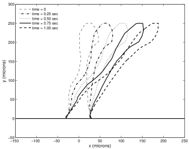
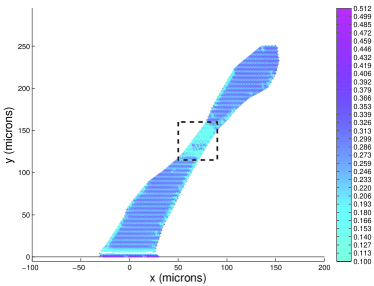
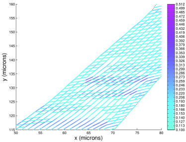
Figure 13: (a) Deformation of the mushroom-shaped biofilm colony at various times in the interval $t\in[0,1]\;\mathrm{s}$. (b) Edges colored according to strain at $t=0.75\;\mathrm{s}$. (c) zoomed view showing edges inside dotted box in (b).

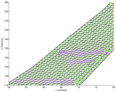
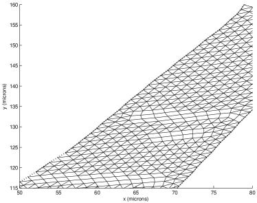
Figure 14: (a) Edges in the stem region inside the dotted box in Fig. 13. Magenta identifies edges with strain above 0.25 and green indicates negative strain, while all other edges are colored black. (b) Spring connectivity after cutting all edges with strain greater than 0.25 at $t=0.75\;\mathrm{s}$.

4.4.2 Equivalent continuum stress-based detachment

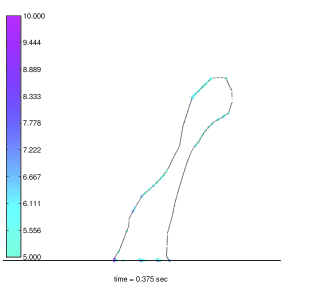
(a) time $=0.375\;\mathrm{s}$

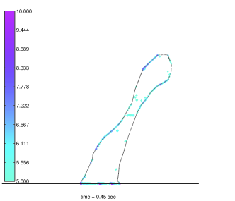
(b) time $=0.45\;\mathrm{s}$

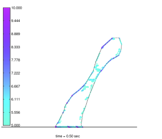
(c) time $=0.50\;\mathrm{s}$

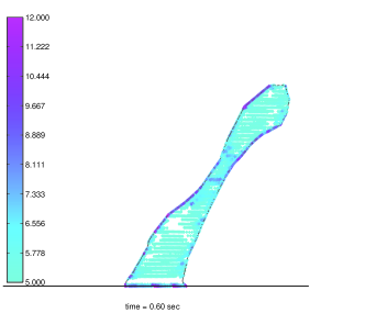
(d) time $=0.60\;\mathrm{s}$

Figure 15: Von Mises stress inside the deformed biofilm at a sequence of times. For purpose of clarity, only points where the stress exceeds $5\mathrm{dyne/cm^{2}}$ are colored.

We next apply the equivalent continuum stress-based detachment strategy to the same problem. The stress tensor components are computed using Eq. (29) after which the von Mises yield stress is computed at each IB node using Eq. (30). Fig. 15 displays the von Mises stress value inside the biofilm region at four time instants during its deformation, where we only color those points with stress above the threshold $5~{}\mathrm{dyne/cm^{2}}$. The von Mises stress has relatively low values throughout most of the colony except in three areas: the stem region, near the base where the colony attaches to the substratum, and in portions of the biofilm-fluid interface that are subject to large fluid shear. The von Mises stress is discontinuous as well as noisy, which is consistent with other numerical simulations of microstructural stress inside granular materials [6, 20]. However, we emphasize that this behaviour is in stark contrast with the apparently smooth von Mises stress field obtained by Towler et al. [54] for a simpler biofilm shape using a finite element simulation.

We make no attempt here to draw any explicit correspondence between results from the strain- and stress-based detachment strategies because the spring strain-based threshold parameter $\varepsilon_{max}$ cannot be translated into a von Mises yield stress value. However, we can still compare the two by simulating detachment for the equivalent continuum stress methodology using the same parameters. This time, we initiate detachment after $0.25\;\mathrm{s}$ of deformation and choose the two distance threshold parameters $\epsilon^{sub}=\epsilon^{ext}=2\;\mathrm{\mbox{$\mu$}m}$ (refer to Section 3.3). This divides the mushroom shaped colony into three zones: in zone 1 near the substratum, the adhesive strength is $\Sigma_{adh}=10~{}\mathrm{dyne/cm^{2}}$; for zone 2 near the biofilm-fluid interface, the interfacial cohesive strength is $\Sigma_{coh}^{ext}=0.1~{}\mathrm{dyne/cm^{2}}$; and for zone 3 in the interior, the cohesive strength is $\Sigma_{coh}^{int}=2.5~{}\mathrm{dyne/cm^{2}}$. Based on these parameter values, Fig. 16 depicts those IB points that will be severed according to the local value of von Mises stress, with the red points indicating detachment in zone 2, while the green points corresponding to detachment in zones 1 and 3. From this figure it is clear that two regions within the colony neck experience complete rupture, which is in agreement with what one would expect from solid mechanics. Furthermore, the detachment criterion is active along the entire biofilm-fluid interface, which corresponds to an erosion process.

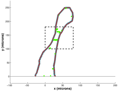
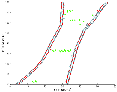
Figure 16: Points where detachment occurs in the biofilm colony at time $t=0.25\;\mathrm{s}$ (zoomed-in view on the right). Detachment parameters are $\epsilon^{sub}=\epsilon^{ext}=2$, $\Sigma_{adh}=10$, $\Sigma_{coh}^{int}=2.5$ and $\Sigma_{coh}^{ext}=0.1$.

In summary, our new detachment strategy based on equivalent continuum stress provides an unambiguous method for performing biofilm detachment that is also consistent with methods employed by other continuum biofilm models. The detachment of any IB point proceeds by cutting of all springs attached to it so that the topology of the spring network remains triangular, thereby avoiding a major disadvantage of the spring strain-based detachment strategy. However, this approach does introduce some additional computational work in each time step for evaluating the equivalent continuum stress and distance functions at each IB node, not to mention maintaining all of the relevant data structures.

4.5 Biofilm deformation and internal stress

This section presents a final series of simulations that study the biofilm stress distribution in more detail and draw specific conclusions regarding the various modes of detachment (sloughing or erosion). We also provide evidence that questions the validity of another class of detachment models based on a detachment speed function.

The steady-state von Mises stress for the Semi20 and Sup75 simulations from the previous section are depicted in Fig. 17 for two values of biofilm spacing, $D_{b}=50$ and $400\;\mathrm{\mbox{$\mu$}m}$. In all cases, the stress is lowest in the interior of the biofilm and largest along the biofilm-fluid and biofilm-wall interfaces, with the absolute maxima occurring on the wall near the leading and trailing corners. We also observe that the proportion of the biofilm experiencing high von Mises stresses increases as the spacing parameter $D_{b}$ increases, which is consistent with the results from Section 4.3. Finally, the stresses experienced in a long, thin colony such as Sup75 are significantly larger (note the increase in the colormap scale by a factor of 10 for plots in the bottom row in Fig. 17).

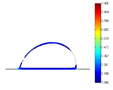
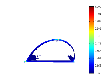
(a) Semi20, $D_{b}=50$	(b) Semi20, $D_{b}=400$
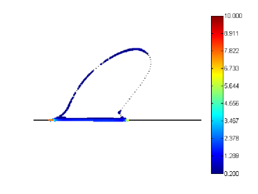
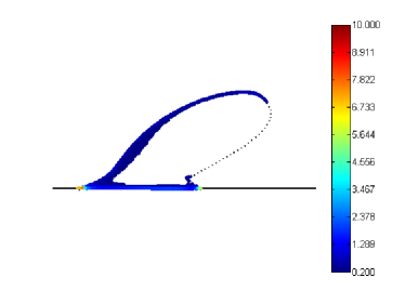
(c) Sup75, $D_{b}=50$	(d) Sup75, $D_{b}=400$

Figure 17: Von Mises yield stress at steady state for cases Semi20 and Sup75, with $\widetilde{\kappa}_{bio}=0.75$ and $D_{b}=50$ and $400\;\mathrm{\mbox{$\mu$}m}$. For ease of visualization, only IB points with stress above a threshold of $0.050~{}\mathrm{dyne/cm^{2}}$ in (a) and (b) and $0.20~{}\mathrm{dyne/cm^{2}}$ in (c) and (d) are shown.

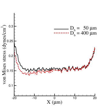
(a) Semi20, biofilm-wall interface

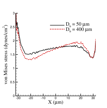
(b) Sup75, biofilm-wall interface

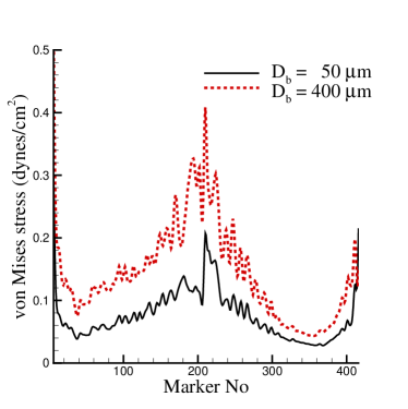
(c) Semi20, biofilm-fluid interface

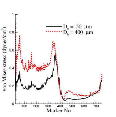
(d) Sup75, biofilm-fluid interface

Figure 18: Von Mises yield stress adjacent to the wall (a,b) and on the biofilm-fluid interface (c,d) for the same simulations as in Fig. 17.

The corresponding plots of von Mises stress along the bottom edge of the colony are shown in Figs. 18(a,b) from which it is clear that the stress peaks at the up/downstream corners. These plots actually terminate a short distance away (5–8 IB points) from the corners because the stress maxima at the corners is 8 to 10 times the value in the interior. We do the same for the stress along the biofilm-fluid interface in Figs. 18(c,d), from which we see that the interfacial shear stress attains a local maximum near the biofilm tip where the fluid shearing force is largest. On comparing the stress plots for the wall and biofilm-fluid interfaces, it is clear that increasing the colony spacing $D_{b}$ has a much more pronounced effect on the biofilm-fluid interface than on the wall stresses. We conclude from these results that for widely-spaced colonies, detachment is more likely to occur by surface erosion than by sloughing from the substratum. This behavior is to be expected since we have used a relatively large value of the spring stiffness connecting the wall and biofilm (compared to the value inside the biofilm). However, if we were to use a lower value to mimic weak wall attachment then we could capture the competition between surface erosion and sloughing modes of detachment, with the dominant mode being determined by the relative sizes of the adhesive ($\Sigma_{adh}$) and exterior cohesive ($\Sigma_{coh}^{ext}$) stress thresholds.

Upon closer investigation of the plots in Fig. 17(c,d), we note that for case Semi20 the von Mises stress increases along the entire exposed biofilm surface as $D_{b}$ increases, whereas in case Sup75 only the left face experiences an increase. This suggests that surface erosion is more uniform for circular colonies, whereas long thin colonies will tend to erode only along the upstream face. Based on this result, and the fact that von Mises stresses are much larger for Sup75, it seems reasonable to suppose that the enhanced surface erosion observed in elongated colonies could be a precursor to formation of streamers that are observed in experiments at low Reynolds number [46, 56]. An in-depth investigation of streamer formation is beyond the scope of this work but could form the basis for an interesting future study based on our IB model.

Additional insight can be gained by comparing plots of interfacial shear stress computed earlier in Figs. 12(a,d) (with $\widetilde{\kappa}_{bio}=0.75$) with the corresponding von Mises stress curves for the same biofilm colonies in Figs. 18(c,d). For the Semi20 case, the interfacial fluid stress and von Mises stress curves have the same general shape along the central portion, with the main difference being that the von Mises stress increases towards the corners whereas the interfacial shear stress does not. For the elongated colony in Sup75, both stresses are asymmetric about the colony apex (near IB point 360) and although both experience a rapid decrease to the right (downstream) of the apex, the upstream behaviour is very different. In particular, the interfacial fluid stress increases gradually on the left toward the apex, while the von Mises stress sustains a relatively large value on the left with a more rapid rise to the maximum.

These differences just mentioned point to an important error in another commonly-used detachment approximation based on a detachment speed function. In this approach, rather than explicitly solving the continuum equations for mechanically-induced detachment, they account for these effects instead by specifying a local speed at which the biofilm-fluid interface recedes into the biofilm [36, 65]. For example, this detachment speed function may depend on the local interfacial shear stress [13] or interfacial curvature [65]. Based on the IB results above in which significant differences occur between fluid shear stress and von Mises stress along the biofilm-fluid interface, it is clear that even for a reasonably stiff biofilm a detachment speed function depending on interfacial shear stress is incapable of correctly capturing detachment dynamics at all points along the interface. It is possible that an alternate speed function could be found that accounts for the variation in von Mises stress along the interface that has been identified in this study and so this would be an worthwhile subject for further study.

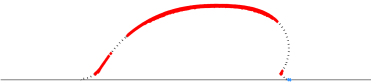
(a) Sup25, $D_{b}=50\;\mathrm{\mbox{$\mu$}m}$

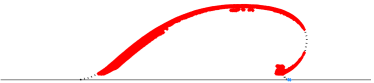
(b) Sup25, $D_{b}=400\;\mathrm{\mbox{$\mu$}m}$

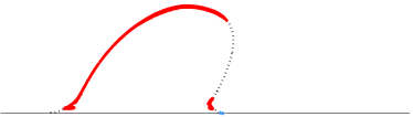
(c) Sup50, $D_{b}=50\;\mathrm{\mbox{$\mu$}m}$

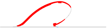
(d) Sup50, $D_{b}=400\;\mathrm{\mbox{$\mu$}m}$

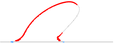
(e) Sup75, $D_{b}=50\;\mathrm{\mbox{$\mu$}m}$

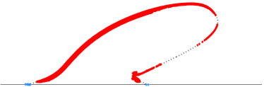
(f) Sup75, $D_{b}=400\;\mathrm{\mbox{$\mu$}m}$

Figure 19: Plots indicating the portion of the biofilm colony (at steady state) that will detach for cases Sup25, Sup50 and Sup75 with $\widetilde{\kappa}_{bio}=0.75$. Sub-figures (a,c,e) have colony spacing $D_{b}=50\;\mathrm{\mbox{$\mu$}m}$, while (b,d,f) have $D_{b}=400\;\mathrm{\mbox{$\mu$}m}$. Other parameters: $\epsilon^{sub}=\epsilon^{ext}=2\;\mathrm{\mbox{$\mu$}m}$, $\Sigma_{coh}^{ext}=0.1\;\mathrm{dyne/cm^{2}}$, $\Sigma_{coh}^{int}=1\;\mathrm{dyne/cm^{2}}$ and $\Sigma_{adh}=5\;\mathrm{dyne/cm^{2}}$.

As a further illustration of the detachment process, Fig. 19 shows the portion of the biofilm that will detach at steady state for cases Sup25, Sup50 and Sup75 with $\widetilde{\kappa}_{bio}=0.75$ and $D_{b}=50$ or $400\;\mathrm{\mbox{$\mu$}m}$. The remaining parameters in the detachment algorithm from Section 3.3 are $\epsilon^{sub}=\epsilon^{ext}=2\;\mathrm{\mbox{$\mu$}m}$, $\Sigma_{coh}^{ext}=0.1\;\mathrm{dyne/cm^{2}}$, $\Sigma_{coh}^{int}=1\;\mathrm{dyne/cm^{2}}$ and $\Sigma_{adh}=5\;\mathrm{dyne/cm^{2}}$. In practice, the removal of IB points by detachment will alter the forces acting on the colony, which in turn induces further deformation; this process repeats until no further detachment is possible. Simulations implementing this alternating detachment/deformation process were conducted for a few selected cases; however, the time step limitation in our IB algorithm ($\Delta t\approx 10^{-5}\;\mathrm{s}$) precluded integrating the solution over the long time intervals required. Consequently, the scope of this work is restricted to introducing the equivalent continuum stress based detachment strategy and validating the results on a range of colony shapes. Efforts to develop a more efficient implementation for a complete deformation and detachment strategy are currently underway with a more efficient IB algorithm and will form the basis for a future publication.

5 Conclusions

We employed a 2D immersed boundary method to simulate the deformation of a periodic array of uniformly-spaced, wall-bounded, weak biofilm colonies in response to a linear shear flow. In order to capture different stages of biofilm growth under mass transfer-limited conditions, we chose a family of biofilms having the same generic shape (sections of a super-ellipse) but with increasing aspect ratios (fixed width, increasing height). Actual biofilm colonies behave mechanically like viscoelastic solids and we mimic this behaviour by replacing the biofilm with a network of Hookean springs corresponding to the edges in a quasi-uniform triangulation of the colony.

We began by performing a parametric study that investigated the effect of colony spacing and spring stiffness on the drag/lift forces and interfacial shear stress acting on the biofilms. The main results of this parametric study can be summarized as follows:

• Varying spring constant: At low shear rates, colonies with even a moderate spring stiffness of $\widetilde{\kappa}_{bio}\geqslant 10$ are able of resisting large deformation forces. Weak biofilm colonies with $\widetilde{\kappa}_{bio}\leqslant 1$ experience increased drag and larger deformations with a maximum displacement in the 10’s of microns. These larger deformations are accompanied by a change in the interfacial shear stress profile wherein stress increases along the upstream face and decreases downstream.

• Varying colony spacing: For low to moderate biofilm stiffness ($\widetilde{\kappa}_{bio}<10$) reducing the colony spacing from 400 to 50 $\mathrm{\mbox{$\mu$}m}$ reduces the drag by as much as 50-100%, accompanied by a change in the shear stress profile along the biofilm-fluid interface. The interfacial shear stress in colonies with large aspect ratio (Sup75) differs significantly from ones with small aspect ratio (Semi20).

• Varying colony shape: It is possible for biofilm colonies to grow into tall structures with large aspect ratio even if they are weak mechanically ($\widetilde{\kappa}_{bio}<10$) owing to the protection from surface erosion afforded by being in close spatial proximity to other colonies. We believe that this result will carry through to 3D (although to a lesser degree) and this is an issue that we plan to investigate further in a future study.

We also developed a new method for initiating biofilm detachment using averaged equivalent continuum stress, which we implemented within our IB framework. We overcame problems encountered in other spring strain based detachment strategies such as in [27] and [1]. The following conclusions can be drawn regarding detachment:

• Variation in von Mises stress: Increasing the spacing between colonies leads to an increased tendency for surface erosion instead of sloughing from the wall. Based on the von Mises stress along the biofilm-fluid interface, we concluded that semi-circular biofilm colonies will undergo roughly uniform surface erosion, while colonies with larger aspect ratios erode predominantly along the upstream face.

• Correlation between fluid stress and von Mises stress: The fluid stress and von Mises yield stress along the biofilm-fluid interface differ substantially. We conclude that biofilm dynamics based on a detachment speed function approach [13, 36] (where detachment speed is a function only of local interfacial fluid stress) cannot capture the actual detachment behaviour resulting from excessive straining. This highlights the importance of using detachment strategies that accurately capture the biofilm mechanics.

The main advantage of our detachment algorithm is that it provides a uniform framework for handling biofilm deformation, surface erosion and sloughing through the use of a continuum mechanics-based detachment model that employs measured biofilm mechanical properties. The primary disadvantage of our approach as implemented herein is the high computational cost; in particular, the small time step required for stability reasons combines with the extra work of simulating detachment to make long-time computations of simultaneous deformation and detachment impractical. We emphasize that this is not a limitation of the immersed boundary approach, but rather our specific implementation that uses a simple explicit time-stepping strategy. We conclude therefore that the full potential of our detachment algorithm can only be realized in combination with either a (semi-)implicit time-stepping approach or an efficient parallel implementation (such as [62]), which will be the subject of future work.

References

- [1] E. Alpkvist and I. Klapper. Description of mechanical response including detachment using a novel particle model of biofilm/flow interaction. Water Sci. Technol., 55(8-9):265, 2007.
- [2] E. Alpkvist and I. Klapper. A multidimensional multispecies continuum model for heterogeneous biofilm development. Bull. Math. Biol., 69(2):765–789, 2007.
- [3] A.P.Boresi and R.J. Schmidt. Advanced mechanics of materials. Wiley New York, 6th edition, 2003.
- [4] J. Arvo. Graphics Gems II, volume 2. Morgan Kaufmann, 1991.
- [5] K. Bagi. Stress and strain in granular assemblies. Mech. Mater., 22(3):165–177, 1996.
- [6] R. Balevičius, I. Sielamowicz, Z. Mroz, and R. Kačianauskas. Investigation of wall stress and outflow rate in a flat-bottomed bin: A comparison of the DEM model results with the experimental measurements. Powder Technol., 214(3):322–336, 2011.
- [7] M. Böl, R. B. Möhle, M. Haesner, T. R. Neu, H. Horn, and R. Krull. 3D finite element model of biofilm detachment using real biofilm structures from CLSM data. Biotechnol. Bioeng., 103(1):177–186, 2009.
- [8] D. C. Bottino and L. J. Fauci. A computational model of ameboid deformation and locomotion. Euro. Biophys. J., 27(5):532–539, 1998.
- [9] J. W. Costerton, P. S. Stewart, and E. P. Greenberg. Bacterial biofilms: A common cause of persistent infections. Science, 284(5418):1318–1322, 1999.
- [10] R. Dillon and L. Fauci. A microscale model of bacterial and biofilm dynamics in porous media. Biotechnol. Bioeng., 68(5):536–547, 2000.
- [11] R. Dillon, L. Fauci, A. Fogelson, and D. Gaver III. Modeling biofilm processes using the immersed boundary method. J. Comput. Phys., 129(1):57–73, 1996.
- [12] R. M. Donlan and W. J. Costerton. Biofilms: survival mechanisms of clinically relevant microorganisms. Clin. Microbiol. Rev., 15(2):167–193, 2002.
- [13] R. Duddu, D. L. Chopp, and B. Moran. A two-dimensional continuum model of biofilm growth incorporating fluid flow and shear stress based detachment. Biotechnol. Bioeng., 103(1):92–104, 2009.
- [14] H. J. Eberl, E. Morgenroth, D. Noguera, C. Picioreanu, B. Rittmann, M. van Loosdrecht, and O. Wanner. Mathematical Modeling of Biofilms, volume 18 of Scientific and Technical Report Series. International Water Association, London, 2006.
- [15] H. J. Eberl, D. F. Parker, and M. C. M. van Loosdrecht. A new deterministic spatio-temporal continuum model for biofilm development. Theor. Med., 3(3):161–175, 2001.
- [16] H. J. Eberl and R. Sudarsan. Exposure of biofilms to slow flow fields: The convective contribution to growth and disinfection. J. Theor. Biol., 253(4):788–807, 2008.
- [17] R. N. Elias, Marcos A. D. Martins, and Alvaro L. G. A. Coutinho. Simple finite element-based computation of distance functions in unstructured grids. Int. J. Numer. Meth. Eng., 72(9):1095–1110, 2007.
- [18] L. J. Fauci and A. McDonald. Sperm motility in the presence of boundaries. Bull. Math. Biol., 57(5):679–699, 1995.
- [19] A. L. Fogelson and R. D. Guy. Platelet–wall interactions in continuum models of platelet thrombosis: formulation and numerical solution. Math. Med. Biol., 21(4):293–334, 2004.
- [20] J. Fortin, O. Millet, and G. De Saxcé. Construction of an averaged stress tensor for a granular medium. Euro. J. Mech. A Solids, 22(4):567–582, 2003.
- [21] D. P. Gaver III and S. M. Kute. A theoretical model study of the influence of fluid stresses on a cell adhering to a microchannel wall. Biophys. J., 75(2):721–733, 1998.
- [22] S. Ghosh and J. M. Stockie. Numerical simulations of particle sedimentation using the immersed boundary method. Commun. Comput. Phys., 2014. Under revision.
- [23] B. E. Griffith. On the volume conservation of the immersed boundary method. Commun. Comput. Phys., 12(2):401–432, 2012.
- [24] B. E. Griffith, R. D. Hornung, D. M. McQueen, and C. S. Peskin. An adaptive, formally second order accurate version of the immersed boundary method. J. Comput. Phys., 223(1):10–49, 2007.
- [25] T. H. Guélon, J. D. Mathias, and P. Stoodley. Advances in biofilm mechanics. In H.-C. Flemming, J. Wingender, and U. Szewzyk, editors, Biofilm Highlights, volume 5 of Springer Series on Biofilms, pages 111–139. Springer, 2011.
- [26] J. F. Hammond, E. J. Stewart, M. J. Solomon, J. G. Younger, and D. M. Bortz. Spatially heterogeneous biofilm simulations using an immersed boundary method with Lagrangian nodes defined by bacterial locations. J. Comput. Phys., 2013. Under revision.
- [27] J. F. Hammond, E. J. Stewart, and J. G. Younger. Modeling and simulation of biofilm fragmentation in fluid flow. J. Comput. Phys., 303:1–24, 2012.
- [28] D. N. Hohne, J. G. Younger, and M. J. Solomon. Flexible microfluidic device for mechanical property characterization of soft viscoelastic solids such as bacterial biofilms. Langmuir, 25(13):7743–7751, 2009.
- [29] J. C. Kissel, P. L. McCarty, and R. L. Street. Numerical simulation of mixed-culture biofilm. J. Environ. Eng., 110(2):393–411, 1984.
- [30] I. Klapper and J. Dockery. Finger formation in biofilm layers. SIAM J. Appl. Math., 62(3):853–869, 2002.
- [31] M. Klausen, A. Aaes-Jørgensen, S. Molin, and T. Tolker-Nielsen. Involvement of bacterial migration in the development of complex multicellular structures in Pseudomonas aeruginosa biofilms. Mol. Microbiol., 50(1):61–68, 2003.
- [32] J. U. Kreft, C. Picioreanu, J. W. T. Wimpenny, and M. C. M. van Loosdrecht. Individual-based modelling of biofilms. Microbiology+, 147(11):2897–2912, 2001.
- [33] M.-C. Lai and C. S. Peskin. An immersed boundary method with formal second-order accuracy and reduced numerical viscosity. J. Comput. Phys., 160(2):705–719, 2000.
- [34] B. Lindley, Q. Wang, and T. Zhang. Multicomponent hydrodynamic model for heterogeneous biofilms: Two-dimensional numerical simulations of growth and interaction with flows. Phys. Rev. E, 85(3):031908, 2012.
- [35] B. A. Lloyd, G. Székely, and M. Harders. Identification of spring parameters for deformable object simulation. IEEE Trans. Vis. Comput. Graphics, 13(5):1081–1094, 2007.
- [36] B. V. Merkey, B. E. Rittmann, and D. L. Chopp. Modeling how soluble microbial products (SMP) support heterotrophic bacteria in autotroph-based biofilms. J. Theor. Biol., 259(4):670–683, 2009.
- [37] Y. Mori. Convergence proof of the velocity field for a Stokes flow immersed boundary method. Commun. Pure Appl. Math., 61:1213–1263, 2008.
- [38] Y. Mori and C. S. Peskin. Implicit second-order immersed boundary methods with boundary mass. Comput. Method. Appl. Mech. Eng., 197(25):2049–2067, 2008.
- [39] C. Nicolella, M. C. M. van Loosdrecht, and J. J. Heijnen. Wastewater treatment with particulate biofilm reactors. J. Biotechnol., 80(1):1–33, 2000.
- [40] A. Ohashi and H. Harada. A novel concept for evaluation of biofilm adhesion strength by applying tensile force and shear force. Water Sci. Technol., 34(5-6):201–211, 1996.
- [41] P.-O. Persson and G. Strang. A simple mesh generator in MATLAB. SIAM Review, 46(2):329–345, 2004.
- [42] C. S. Peskin. Numerical analysis of blood flow in the heart. J. Comput. Phys., 25(3):220–252, 1977.
- [43] C. S. Peskin. The immersed boundary method. Acta Numerica, 11:479–517, 2003.
- [44] C. Picioreanu, M. C. M. van Loosdrecht, and J. J. Heijnen. Two-dimensional model of biofilm detachment caused by internal stress from liquid flow. Biotechnol. Bioeng., 72(2):205–218, 2001.
- [45] W. H. Press. Numerical Recipes in Fortran 77: The Art of Scientific Computing, volume 1. Cambridge University Press, 1992.
- [46] R. Rusconi, S. Lecuyer, N. Autrusson, L. Guglielmini, and H. A. Stone. Secondary flow as a mechanism for the formation of biofilm streamers. Biophys. J., 100(6):1392–1399, 2011.
- [47] P. Seeluangsawat. 3-D computational investigation of viscoelastic biofilms using GPUs. PhD thesis, Department of Mathematics, University of South Carolina, Columbia, SC, 2011.
- [48] X. Shi and X. Zhu. Biofilm formation and food safety in food industries. Trends Food Sci. Technol., 20(9):407–413, 2009.
- [49] B. Smith, B. Vaughan, and D. Chopp. The extended finite element method for boundary layer problems in biofilm growth. Commun. Appl. Math. Comput. Sci., 2(1):35–56, 2007.
- [50] J. M. Stockie. Analysis and computation of immersed boundaries, with application to pulp fibers. PhD thesis, Department of Mathematics, University of British Columbia, 1997.
- [51] J. M. Stockie. Modelling and simulation of porous immersed boundaries. Comput. Struct., 87(11-12):701–709, 2009.
- [52] R. Sudarsan, K. Milferstedt, E. Morgenroth, and H. J. Eberl. Quantification of detachment forces on rigid biofilm colonies in a roto-torque reactor using computational fluid dynamics tools. Water Sci., 52(7):149–154, 2005.
- [53] D. Taherzadeh, C. Picioreanu, and H. Horn. Mass transfer enhancement in moving biofilm structures. Biophys. J., 102(7):1483–1492, 2012.
- [54] B. W. Towler, A. Cunningham, P. Stoodley, and L. McKittrick. A model of fluid-biofilm interaction using a Burger material law. Biotechnol. Bioeng., 96(2):259–271, 2007.
- [55] B. W. Towler, C. J. Rupp, A. B. Cunningham, and P. Stoodley. Viscoelastic properties of a mixed culture biofilm from rheometer creep analysis. Biofouling, 19(5):279–285, 2003.
- [56] A. Valiei, A. Kumar, P. P. Mukherjee, Y. Liu, and T. Thundat. A web of streamers: biofilm formation in a porous microfluidic device. Lab on a Chip, 12(24):5133–5137, 2012.
- [57] G. D. Vo, E. Brindle, and J. Heys. An experimentally validated immersed boundary model of fluid-biofilm interaction. Water Sci. Technol., 61(12):3033–3040, 2010.
- [58] G. D. Vo and J. Heys. Biofilm deformation in response to fluid flow in capillaries. Biotechnol. Bioeng., 108(8):1893–1899, 2011.
- [59] V. R. Voller. Basic Control Volume Finite Element Methods for Fluids and Solids. World Scientific, Singapore, 2009.
- [60] Q. Wang and T. Zhang. Review of mathematical models for biofilms. Solid State Commun., 150(21-22):1009–1022, 2010.
- [61] O. Wanner and W. Gujer. A multispecies biofilm model. Biotechnol. Bioeng., 28(3):314–328, 1986.
- [62] J. K. Wiens and J. M. Stockie. An efficient parallel immersed boundary algorithm using a pseudo-compressible fluid solver. J. Comput. Phys., 281:917–941, 2015.
- [63] H. A. R. Williams, L. J. Fauci, and D. P. Gaver. Evaluation of interfacial fluid dynamical stresses using the immersed boundary method. Disc. Contin. Dyn. Syst. B, 11(2):519–540, 2009.
- [64] J. W. T. Wimpenny and R. Colasanti. A unifying hypothesis for the structure of microbial biofilms based on cellular automaton models. FEMS Microbiol. Ecol., 22(1):1–16, 1997.
- [65] J. D. B. Xavier, C. Picioreanu, and M. C. M. van Loosdrecht. A general description of detachment for multidimensional modelling of biofilms. Biotechnol. Bioeng., 91(6):651–669, 2005.
- [66] J. Xu, R. Sudarsan, G. A. Darlington, and H. J. Eberl. A computational study of external shear forces in biofilm clusters. In 22nd International Symposium on High Performance Computing Systems and Applications, pages 139–145, Québec, Canada, 2008. IEEE.
- [67] T. Zhang, N. Cogan, and Q. Wang. Phase-field models for biofilms. II. 2-D numerical simulations of biofilm-flow interaction. Commun. Comput. Phys., 4(1):72–101, 2008.
- [68] P. Zhao and J. C. Heinrich. Front-tracking finite element method for dendritic solidification. J. Comput. Phys., 173(2):765–796, 2001.