Spectral functions and time evolution from the Chebyshev recursion

Abstract

We link linear prediction of Chebyshev and Fourier expansions to analytic continuation. We push the resolution in the Chebyshev-based computation of $T=0$ many-body spectral functions to a much higher precision by deriving a modified Chebyshev series expansion that allows to reduce the expansion order by a factor $\sim\frac{1}{6}$. We show that in a certain limit the Chebyshev technique becomes equivalent to computing spectral functions via time evolution and subsequent Fourier transform. This introduces a novel recursive time evolution algorithm that instead of the group operator $e^{-iHt}$ only involves the action of the generator $H$. For quantum impurity problems, we introduce an adapted discretization scheme for the bath spectral function. We discuss the relevance of these results for matrix product state (MPS) based DMRG-type algorithms, and their use within dynamical mean-field theory (DMFT). We present strong evidence that the Chebyshev recursion extracts less spectral information from $H$ than time evolution algorithms when fixing a given amount of created entanglement.

I Introduction

Expanding the spectral density $A(\omega)$ of an operator $H$ in the monomes $\omega^{n}$ via the moments

$$\mu_{n}^{\text{mon}}=\int d\omega\,A(\omega)\omega^{n},$$

is a tool that originates in the early days of quantum mechanics.(Weiße et al., 2006) Computing these moments iteratively though is numerically unstable(Gautschi, 1967, 1968) and one replaced expansions in $\omega^{n}$ by expansions in such polynomials $p_{n}(\omega)$ of degree $n$ that can be stably computed.(Gautschi, 1970; Sack and Donovan, 1971) A prominent example for $p_{n}(\omega)$ are Chebyshev polynomials, whose associated three-term recursion is stable as it does not admit a so-called minimal(Gautschi, 1967) solution.

After the development of stable recursions the next step in the mid 1990s was the introduction of kernels that damp the erroneous Gibbs oscillations of truncated polynomial expansions of discontinuous functions,(Silver and Röder, 1994; Wang, 1994; Wang and Zunger, 1994) which lead to the kernel polynomial approximation. It deals with redefined series expansions that represent the convolution of the expanded function with a broadening kernel, like a Gaussian or Lorentzian. This technique has been reviewed in Ref. Weiße et al., 2006 and more recently in Ref. Lin et al., 2013 from a numerical linear algebra perspective.

In this paper, we drop the idea of such broadening kernels in frequency space or the equivalent damping or windowing kernels in the associated Fourier or Chebyshev expansions. Instead, we employ the fundamentally different technique of linear prediction.(Press et al., 2007) Linear prediction is a linear recursive reformulation (Appendix C) of the non-linear problem to fit the surrogate function

$$g(t)=\sum_{i}\alpha_{i}e^{i\omega_{i}t},\quad\alpha_{i},\omega_{i}\in\mathbb{C},~{}t\in\mathbb{R},$$ (1)

to given numerical data $\{t_{n},g_{n}\}$. Due to linearity, linear prediction is able to treat superpositions of hundreds of terms, and by that reliably extracts much information about an underlying function from its local knowledge $\{t_{n},g_{n}\}$. In order for this to be meaningful, the underlying function, e.g. a Green’s function, must be compatible with (1).

In particular, we note that (1) can serve as an ansatz for analytic continuation of a zero-temperature Green’s function

$$G(t)=-i\langle\psi_{0}|e^{-i(H-E_{0})t}|\psi_{0}\rangle,$$ (2)

where $|\psi_{0}\rangle$ is a single-particle excitation of the groundstate $|E_{0}\rangle$ of $H$, for example the creation of a fermion $|\psi_{0}\rangle=c^{\dagger}|E_{0}\rangle$. Note that in the case of fermions, (2) describes only the $t>0$ contribution (then usually more precisely denoted $G^{>}(t)$) of the full fermionic Green’s function. $G(t)$ is analytic everywhere in the complex plane except for $t\rightarrow i\infty$ and thereby allows for an analytic continuation of $G(t)$ from a local description $\{t_{n},G(t_{n})\}$ to the domain $[t_{0},\infty)$. This analytic continuation is highly different from the ill-conditioned problem of continuing the frequency-space represented Green’s function from a domain in the complex plane (e.g. the imaginary-frequency axis or a parallel of the real-frequency axis) to the real-frequency axis, where the frequency-space Green’s function has poles.

In the context of Green’s functions, linear prediction has for the first time been used to extrapolate the time evolution of the spin structure factor in the one dimensional Heisenberg model.(White and Affleck, 2008; Barthel et al., 2009) While for the spin-$1$ model it was clear that the ansatz (1) is justified as the time evolution is dominated by a small number of magnons whose excitation energies correspond directly to the frequencies $\omega_{i}$ in (1),(White and Affleck, 2008) this was not the case for the spin-$\frac{1}{2}$ model.(Barthel et al., 2009) In the latter, spinons dominate which lead to an (infinitely) high number of poles on the real-frequency axis, and the direct correspondence of pole energies and frequencies $\omega_{i}$ in (1) is lost. Still the ansatz works(Barthel et al., 2009) in an approximate sense by extracting effective frequencies.

For the computation of spectral functions, the use of linear prediction for the time evolution of Green’s functions provides a highly attractive alternative approach to the usual damping or windowing in real-time or broadening in frequency space: an approach that enhances resolution in frequency space. Up to now, it is not entirely clear in which cases this is controlled. On the other hand, the approach of damping the truncated series expansion cannot be considered controlled, too: Although a broadened function $f_{\eta}(\omega)$, which is for Gaussian broadening given by $f_{\eta}(\omega)=\frac{1}{\eta\sqrt{2\pi}}\int d\omega^{\prime}e^{-(\omega^{\prime}-\omega)^{2}/2\eta^{2}}f(\omega^{\prime})$, converges uniformly to the underlying original function $f(\omega)$ for $\eta\rightarrow 0$, extraction of information (deconvolution) from $f_{\eta}(\omega)$ about $f(\omega)$ is uncontrolled as it corresponds to the problem of analytic continuation from a domain in the complex plane to the real axis.

Recently, Ref. Ganahl et al., 2014a suggested to extrapolate the Chebyshev expansion of a spectral function using linear prediction, albeit only justified by the empirical success. In the remainder of this introduction, we place these results in the context of the preceding discussion, and by that put this approach on more firm grounds.

I.1 Chebyshev and Fourier transformation basics

The Chebyshev polynomials of the first kind

$$T_{n}(x)=\cos\left(n\arccos(x)\right)$$ (3)

can be generated by the recursion

$$T_{n}(x)=2xT_{n-1}(x)-T_{n-2}(x),\quad T_{1}=x,\quad T_{0}=1,$$ (4)

which is numerically stable if $\left|x\right|\leq 1$. Chebyshev polynomials are orthonormal with respect to the weighted inner product

$$\int_{-1}^{1}dx\,w_{n}(x)T_{m}(x)T_{n}(x) =\delta_{nm},$$ (5a)

$$w_{n}(x) =\frac{2-\delta_{n0}}{\pi\sqrt{1-x^{2}}}.$$ (5b)

Any integrable function $f(x)|_{x\in[-1,1]}$ can be expanded in $T_{n}(x)$

$$f(x) =\sum_{n=0}^{\infty}w_{n}(x)\mu_{n}T_{n}(x),$$ (6a)

$$\mu_{n} =\int_{-1}^{1}dx\,T_{n}(x)f(x),$$ (6b)

where the definition of the so-called Chebyshev moments $\mu_{n}$ via the non-weighted inner product (6b) follows when applying $\int_{-1}^{1}dx\,T_{m}(x)\dots$ to both sides of (6a).

Analogously, any integrable function $f(\omega)|_{\omega\in[-\frac{a}{2},\frac{a}{2}]}$, where $a\in\mathbb{R}$, can be expanded in a Fourier series

$$f(\omega) =\frac{1}{2a\pi}\sum_{n=-\infty}^{\infty}e^{i\omega t_{n}}f(t_{n}),$$ (7a)

$$f(t_{n}) =\int_{-a/2}^{a/2}d\omega\,e^{-i\omega t_{n}}f(\omega),\quad t_{n}=\frac{n}{a},$$ (7b)

which represents a Fourier transform for $a\rightarrow\infty$.

I.2 Expansion of a spectral function

Consider now the expansion of the spectral function $A(\omega)$ of a Hamilton operator $H$ with respect to a reference energy $E_{\text{ref}}$ and a state $|\psi_{0}\rangle$ as in (2)

$$A(\omega) =\langle\psi_{0}|\delta(\omega-(H-E_{\text{ref}}))|\psi_{0}\rangle.$$ (8)

The spectral function is related to the Green’s function of (2) via its Fourier transform: $A(\omega)=-\frac{1}{\pi}\text{Im}\,G(\omega+i0^{+})$.

The coefficients of the Fourier expansion can be computed by inserting an identity of eigenstates $\sum_{i}|E_{i}\rangle\langle E_{i}|$ in the integral over the delta function $\delta(\omega-(H-E_{\text{ref}}))$

$$f(t_{n}) =\int_{-a/2}^{a/2}d\omega\,e^{-i\omega t_{n}}A(\omega)=\langle\psi_{0}|\psi(t_{n})\rangle,$$ (9a)

$$|\psi(t_{n})\rangle =e^{-i(H-E_{\text{ref}})t_{n}}|\psi_{0}\rangle,\quad t_{n}=\frac{n}{a}.$$ (9b)

In order for (9) to hold true, $a$ must be chosen large enough for that the support of $A(\omega)$ is contained in $[-\frac{a}{2},\frac{a}{2}]$. A sufficient condition for that is $\text{spec}(H-E_{\text{ref}})\subset[-\frac{a}{2},\frac{a}{2}]$, which is possible as we consider operators $H$ with bounded spectra. Eq. (9b) makes it obvious that $a$ has the meaning of an inverse time step.

To compute the coefficients for the Chebyshev expansion, we need to consider a spectral function whose support is contained in $[-1,1]$. For this, introduce a rescaled and shifted version of $H$ with appropriately chosen constants $a$ and $b$

$$\mathcal{H}_{a,b}=\frac{H-E_{\text{ref}}}{a}+b,\quad x=\frac{\omega}{a}+b,$$ (10)

where $a$ can again be considered an “inverse time step” and $\mathcal{H}$ is dimensionless. Note that in Ref. Wolf et al., 2014a, the definition of $b$ differed from the one here by a factor $a$. Then

$$\mathcal{A}_{a,b}(x)=\langle\psi_{0}|\delta(x-\mathcal{H}_{a,b})|\psi_{0}\rangle$$ (11)

yields the original spectral function via $A(\omega)=\frac{1}{a}\mathcal{A}\big{(}\tfrac{\omega}{a}+b\big{)}$, where we omitted to specify the indices $a,b$, as in most of the rest of this paper. The Chebyshev moments for $\mathcal{A}(x)$ can be computed analogously to the Fourier coefficients (9)

$$\mu_{n} =\int_{-1}^{1}dx\,\mathcal{A}(x)T_{n}(x)=\langle\psi_{0}|\psi_{n}\rangle,$$ (12a)

$$|\psi_{n}\rangle =T_{n}(\mathcal{H})|\psi_{0}\rangle.$$ (12b)

Inserting the recursive definition (4) of $T_{n}(\mathcal{H})$ in the definition (12b) of $|\psi_{n}\rangle$, one obtains a practical calculation scheme for the power series expansion of $T_{n}(\mathcal{H})$, and by that for the Chebyshev states $|\psi_{n}\rangle$ in (12):

$$|\psi_{n}\rangle=2\mathcal{H}|\psi_{n-1}\rangle-|\psi_{n-2}\rangle,\quad|\psi_{1}\rangle=\mathcal{H}|\psi_{0}\rangle.$$ (13)

I.3 Analytic continuation

A comparison of (9b) and (12b) clarify why linear prediction is an equally justified approach for a Chebyshev as for a Fourier expansion.

Rewriting the “evolution operators” that appear in (9b) and (12b) as

$$\exp(-in\mathcal{H}_{a,b=0})\qquad\text{and}\qquad\cos(n\arccos(\mathcal{H}_{a,b}))$$ (14)

makes it clear that we deal with analytic functions of $n$ if we consider $n$ as a continuous complex variable. By (9a) and (12a), this makes the Fourier and the Chebyshev coefficients $f(t_{n})$ and $\mu_{n}$ analytic functions of $n$, too. In addition, $\text{Re}\,\exp(-in\mathcal{H}_{a,b})=\cos(n\mathcal{H}_{a,b})$ shows that the real part of the functional dependence of the time evolution operator on $n$ is the same as for the “Chebyshev evolution operator”, when neglecting a redefinition of oscillations frequencies. As this redefinition can be accounted for by the fitting procedure, the particular form of the surrogate function $g(t)$ in (1) is equally suited to analytically continue both types of expansions. A fundamental theorem from complex analysis then tells us that if linear prediction provides us with a function $g(t)$ that locally agrees with $f(t_{n})$ or $\mu_{n}$, we know that this function globally agrees with $f(t_{n})$ or $\mu_{n}$. Of course, in practice these arguments are to be taken with care, as we will never numerically find a function $g(t_{n})$ that agrees exactly with the local data $\{g_{n},t_{n}\}$.

I.4 Outline of the paper

We will first study the convergence properties of the Chebyshev expansion of discontinuous (spectral) functions in the thermodynamic limit. This allows to derive a new scheme for a Chebyshev series defintion that leads to exponential convergence and allows to reduce expansion orders in practical calculations by a factor $\sim\frac{1}{6}$ (Sec. II). We then apply these results to the computation of spectral functions for finite systems (Sec. III), and discuss the relevance for matrix product state (MPS) based computations (Sec. IV). After that, we describe the approximate equivalence of the Chebyshev recursion to time evolution and show how this leads to a novel time evolution algorithm (Sec. V). Finally, we conclude the paper (Sec. VI).

II Spectral functions in the thermodynamic limit

A spectral function for a system of finite size $L$ has a finite-size peak structure due to an agglomeration of eigenvalues that is not present in the thermodynamic limit. In a weakly interacting system, this agglomeration happens around the positions of the eigenvalues of the corresponding noninteracting (single-particle) system. This argument gives us the best, though still very rough, estimate $W_{\text{single}}/L$ for the spacing of finite-size peaks, where $W_{\text{single}}$ is the single-particle bandwidth. At a much smaller spacing than that, spectral functions have an underlying delta peak structure, as is obvious from definition (8), which can be rewritten as

$$A(\omega) =\sum_{i}W_{i}\,\delta(\omega-(E_{i}-E_{\text{ref}})),$$ (15)

with weights $W_{i}=\left|\langle\psi_{0}|E_{i}\rangle\right|^{2}$. The delta peak structure merges to a (section-wise) smooth function only in the thermodynamic limit.

Expanding the spectral function of a finite-size system in orthogonal polynomials is a very efficient way to not resolve either finite-size peaks or the delta peak structure, but to extract only the smooth function of the thermodynamic limit, as e.g. discussed in Ref. Wolf et al., 2014a. It is this function of the thermodynamic limit that we are interested in, and for which we start our discussion.

II.1 Discontinuity of spectral functions

The state $|\psi_{0}\rangle$ and the energy $E_{\text{ref}}$ in (15) are generally associated to the ground state of a certain symmetry sector $N$ of $H$, which for fermions is typically a particle number. The reference energy for $|\psi_{0}\rangle=c^{\dagger}|E_{0}\rangle$ then is the Fermi energy, which is the ground state energy $E_{\text{ref}}=E_{0}^{N-1}$ of the contiguous symmetry sector of $|\psi_{0}\rangle$ (or $E_{\text{ref}}=E_{0}^{N+1}$ for a hole excitation). The weights $W_{i}=\left|\langle\psi_{0}|E_{i}\rangle\right|^{2}$ in the spectral function (15) can be non-zero only for eigenstates $|E_{i}\rangle$ and eigenvalues $E_{i}$ from the sector $N$. The particular meaning of $E_{\text{ref}}$ as a ground state energy then implies that even if the global spectral function

$$A_{\text{global}}(\omega)=\sum_{i}\delta(\omega-(E_{i}-E_{\text{ref}}))$$ (16)

is smooth, the weights $W_{i}$ generally introduce a discontinuity at $\omega=0$ (we use the term global here, as $|\psi_{0}\rangle$ usually is a local excitation associated with a certain quantum number).

II.2 Convergence of Chebyshev series expansions

The convergence of the Chebyshev moments $\mu_{n}\rightarrow 0$ of a function $f(x)$ in the limit $n\rightarrow\infty$ can be characterized by the degree of differentiability of $f(x)$, similar to a Fourier expansion.(Boyd, 2001) Let $k$ denote the highest integer for which the $k$th derivative of $f(x)$ is integrable: If $f(x)$ is smooth ($k=\infty$), the envelope of $\mu_{n}$ converges exponentially to zero with respect to $n$; if $f(x)$ is a step function ($k=1$), the envelope converges algebraically with $\frac{1}{n}$; and if $f(x)$ is a delta function, the envelope remains constant. In general, the order of convergence is at least $\frac{1}{n^{k}}$. Although in Ref. Boyd, 2001, this is stated for moments computed with the weighted inner product (5b), it also holds for moments computed using (6b) (see Appendix A). In practice, we are not interested in the limit $n\rightarrow\infty$, but rather in intermediate values of $n$: but also here, the degree of differentiability of $A(\omega)$ helps us to learn something about the convergence of $\mu_{n}$.

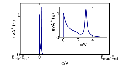
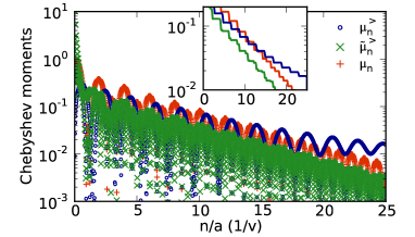
Figure 1: (Color online) Top: Typical example of a discontinuous spectral function due to the restriction to a given symmetry sector. In this case, this is the particle contribution of the spectral function of the single-impurity Anderson model (SIAM) with semi-elliptic bath density of states of half-bandwidth $2v$ and interaction $U/v=4$,(Raas et al., 2004) taken from Ref. Wolf et al., 2014a. The spectral function is given by (8) using $|\psi_{0}\rangle=c^{\dagger}|E_{0}\rangle$, where $|E_{0}\rangle$ denotes the half-filled ground state and $E_{\text{ref}}$ is the Fermi energy $E_{0}$. Here, only the shape of the scalar function is of importance, therefore we postpone the model definition to (30). The same spectral function is obtained for the local density of states of the first site for spinless fermions hopping on a semi-infinite chain with tunneling $v$ and and an interaction of $U/v=4$ that acts only on the first site. Bottom: Comparison of convergence of the Chebyshev moments of $A^{>}(\omega)$ with its redefinitions $\widetilde{A}^{>}(\omega)$ and $A(\omega)$, giving rise to moments $\mu_{n}^{>}$, $\widetilde{\mu}_{n}^{>}$ and $\mu_{n}$, respectively. The full spectral function (18) for this example is $A(\omega)=A^{>}(\omega)+A^{>}(-\omega)$ as here, $A^{<}(\omega)=A^{>}(\omega)$ due to particle-hole symmetry. All of this is for the setup $b=0$ using a rescaling of $a=100v$ in (10).

Consider a typical discontinuous spectral function $A^{>}(\omega)$ as shown in the top panel of Fig. 1. Its corresponding Chebyshev moments $\mu_{n}^{>}$ are computed by numerically integrating (6b) and shown in the bottom panel of Fig. 1 as blue circles. The blue line in the inset shows the envelope of $\mu_{n}^{>}$, which evidently decreases algebraically to zero.

Now note that continuity of $A^{>}(\omega)$ at $\omega=0$ can easily be restored by defining

$$\widetilde{A}^{>}(\omega)=A^{>}(\omega)-A^{>}(0).$$ (17)

The green crosses (lines) in the bottom panel of Fig. 1 show that the Chebyshev moments $\widetilde{\mu}_{n}^{>}$ of $\widetilde{A}^{>}(\omega)$ converge exponentially for the values of $n$ considered in the plot, i.e., qualitatively differently than $\mu_{n}^{>}$. This is observed although $\widetilde{A}^{>}(\omega)$ is not smooth, but only once differentiable (kink in first derivative at $\omega=0$).

While the construction of $\widetilde{A}^{>}(\omega)$ is completely general, for the particular case of a fermionic spectral function, another way of constructing a continuous function from $A^{>}(\omega)$ has been favored: In the appendix of Ref. Holzner et al., 2011, it was mentioned that the Chebyshev expansion of the full spectral function

$$A(\omega) =A^{>}(\omega)+A^{<}(-\omega),$$ (18)

$$A^{\gtrless}(\omega) =\langle\psi_{0}^{\gtrless}|\,\delta(\omega-(H-E_{0}))|\psi_{0}^{\gtrless}\rangle,$$

obtained by summing over particle ($>$) and hole ($<$) contributions, is much better suited for a Chebyshev expansion than $A^{\gtrless}(\omega)$, as it lacks the discontinuity. In Ref. Ganahl et al., 2014a it was then pointed out that the full $A(\omega)$ is smooth and therefore, Chebyshev moments should decrease exponentially, which would allow to use linear prediction. In general, it is not true that $A(\omega)$ is smooth, due to the possibility of van Hove singularities, as appear e.g. for the $U=0$ case of the spectral function of the single impurity Anderson model (SIAM) (see Appendix B, Fig. 11). Still, $A(\omega)$ is likely to be smooth, and for the present example, it is. The bottom panel of Fig. 1 therefore shows that the Chebyshev moments $\mu_{n}$ for $A(\omega)$ decrease at the same exponential rate as the moments $\widetilde{\mu}_{n}^{>}$ of $\widetilde{A}^{>}(\omega)$.

The statements about the qualitatively different convergence behaviors of $A^{>}(\omega)$, $\widetilde{A}^{>}(\omega)$ and $A(\omega)$ are confirmed for further typical examples in Appendix B.

II.3 Comparison of setups $b=0$ and $b\simeq-1$

In Ref. Wolf et al., 2014a, we pointed out that the choice $b=0$ in (10) is computationally much less efficient than the choice $b\simeq-1$ (called “$b\simeq-a$” in Ref. Wolf et al., 2014a). Whereas constructing a Chebyshev expansion of the full spectral function $A(\omega)$ requires choosing $b=0$, this is not the case for $\widetilde{A}(\omega)$. For $\widetilde{A}(\omega)$, we can therefore use the exponential rate of convergence to quantify the amount of spectral information that the Chebyshev recursion extracts from $H$ in the setups $b=0$ and $b\simeq-1$, and by that understand the observations of Ref. Wolf et al., 2014a quantitatively.

The key observation to make is that the integral

$$\mu_{n}^{>}=\int_{-1}^{1}dx\,\mathcal{A}_{a,b}^{>}(x)T_{n}(x)$$ (19)

extracts a highly different amount of information about the structure of $A^{>}(\omega)$ depending on how $a$ and $b$ in (10) are chosen when generating $\mathcal{A}_{a,b}^{>}(x)$.

Throughout the whole paper, we keep $a=100v$ fixed to guarantee the numerical stability of the Chebyshev recursion for the typical system sizes of around $L\geq 80$ that are large enough to display “thermodynamic limit behavior”. If we chose $a$ smaller, we could only stably compute “small” systems or we would have to resort to the technique of energy truncation, which is strongly prone to errors.(Holzner et al., 2011) Furthermore, in the MPS context, it is important to compare only computations in which $a$ is kept constant: constant $a$ means constant effective hopping energies $\frac{v}{a}$ in $\mathcal{H}$, and by that a constant amount of entanglement production in a single iteration step of (13). The parameter $b$, by contrast, can be chosen freely without affecting the numerical stability, and in principle, without affecting entanglement production in MPS computations.

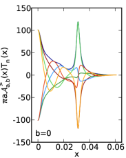
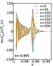
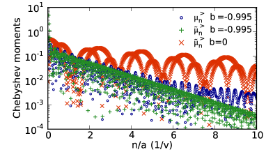
Figure 2: (Color online) Top: Integrand for computation of moments for the spectral function shown in Fig. 1. in the two setups $b=0$ (left) and $b=-0.995$ (right). Bottom: Comparison of convergence of moments computed with the integrands shown in the top panels. In all of that, $a=100v$.

The top panels of Fig. 2 show the convolution of $\mathcal{A}_{a,b}^{>}(x)$ with Chebyshev polynomials $T_{n}(x)$ of different degree $n$ for the two setups $b=0$ and $b=-0.995\simeq-1$. The highly increased oscillation frequency that is evident in the setup $b=-0.995$ can be understood by looking at the natural stretching of the frequency scale of Chebyshev polynomials close to the boundaries of $[-1,1]$. Expressing the integral (19) by substituting $x=\cos\theta$

$$\mu_{n}^{>}=-\int_{\pi}^{0}d\theta\,\mathcal{A}_{a,b}^{>}(\cos\theta)\cos(n\theta)\sin\theta,$$ (20)

one arrives at a convolution with the regularly oscillating $\cos(n\theta)$. Consider now the interval of width $0.05$ on $[-1,1]$, which corresponds to the (single-particle) support of $\mathcal{A}_{a,b}^{>}(x)$ in the example of Fig. 2. By computing the integral widths under the map $x=\cos\theta$, one learns that placing the support in the “boundary region” $[-0.995,-0.95]$, as results for $b=-0.995$, increases the resolution by a factor $\sim 6.4$ compared to placing it in the “center region” $[0,0.05]$, as results for $b=0$. These effects are well known boundary effects of the Chebyshev polynomials that are exploited also in the solution of differential equations.(Boyd, 2001)

The bottom panel of Fig. 2 shows the Chebyshev moments obtained in the $b=-0.995$ setup, for $A^{>}(\omega)$ (blue circles) and for $\widetilde{A}^{>}(\omega)$ (green pluses). As mentioned before, for this setup, no Chebyshev expansion of the full spectral function $A(\omega)$ is possible. Instead, we compare the $b=-0.995$ results to the $b=0$ results, depicted as red crosses. It is evident that the Chebyshev expansion in the $b=-0.995$ setup converges much faster than the one in the $b=0$ setup. After $n=1000$ iterations, the magnitude differs by more than 100.

This difference directly appears in the error of the Chebyshev series, as stated by the following general rule: the order of the error $\varepsilon$ of a Chebyshev (or Fourier) series representation of a function that is truncated at $n=N$ can be estimated by (see Ref. Boyd, 2001, Chap. 2.12)

$$\varepsilon =\mathcal{O}(\mu_{N})\quad\text{ if $\mu_{n}$ converges exponentially},$$ (21a)

$$\varepsilon =\mathcal{O}(N\mu_{N})\quad\text{ if $\mu_{n}$ converges algebraically}.$$ (21b)

II.4 Linear prediction for the Chebyshev expansion

The main motivation for studying the convergence of different Chebyshev expansions in the previous sections lies in the possibility to extrapolate exponentially decreasing sequences with linear prediction. As discussed in the introduction, the latter allows an extremely high gain in resolution, if its application is justified. For details on linear prediction, see Appendix C.

In what follows, we compare the known approach of using linear prediction for the Chebyshev expansion of $A(\omega)$, as suggested in Ref. Ganahl et al., 2014a, with the new approach of extrapolating the Chebyshev expansion of $\widetilde{A}^{>}(\omega)$.

We first compute the Chebyshev moments of the step function that has the discontinuity of $A^{>}(\omega)$ at $\omega=0$, which transforms to $x=-b$ for $\mathcal{A}^{>}(x)$, as

$$\mu_{n}^{{}_{\text{step}}} =\int_{-b}^{1}dx\,T_{n}(x)$$ (22)

$$=\frac{1}{2}\Big{(}\frac{\cos[(n+1)\arccos x]}{n+1}$$

$$\qquad~{}-\frac{\cos[(n-1)\arccos x]}{n-1}\Big{)}\Big{|}_{-b}^{1}.$$

The Chebyshev moments of $\widetilde{A}^{>}(x)$ are then given by

$$\widetilde{\mu}_{n}^{>}=\mu_{n}^{>}-A^{>}(0)\mu_{n}^{{}_{\text{step}}}$$ (23)

and are accessible by linear prediction, as they decrease exponentially.

The core problem in this new approach is that the value $A^{>}(0)$ of the spectral function is, in general, unknown prior to linear prediction. But it fulfills the following self-consistency problem, which can be iteratively solved: Choosing a start value $A_{0}^{>}(0)$ for $A^{>}(0)$, we compute $\widetilde{\mu}_{n}$, extrapolate the sequence up to convergence, and then use the extrapolated sequence to reconstruct $A^{>}(\omega)$, which provides us with a new value $A_{1}^{>}(0)$. We repeat the procedure until the new and the old version $A_{i}^{>}(0)$ and $A_{i+1}^{>}(0)$ agree. This procedure is found to converge stably and quickly for all examples studied (see also Appendix B).

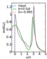
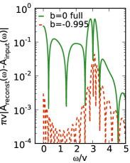
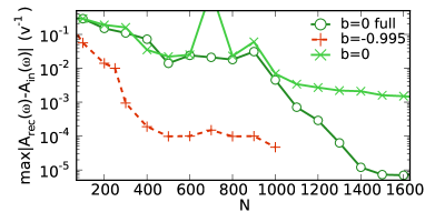
Figure 3: (Color online) Top: Input spectral function and reconstructed spectral functions using linear prediction for $N=200$ computed Chebyshev moments. We compare our proposal with the original proposal,(Ganahl et al., 2014a) where for the $b=0$ setup the expansion of the full spectral function was extrapolated. Left: In the first case, we use the Chebyshev expansion of $\widetilde{A}^{>}(\omega)$ in the $b=-0.995$ setup (red dashed lines), and in the second, we use the Chebyshev expansion of the full spectral function $A(\omega)$ in the $b=0$ setup (solid green line). Right: Error of these functions $|A_{\text{reconst}}(\omega)-A_{\text{input}}(\omega)|$ for both setups. Bottom: The error $\max_{\omega\geq 0}|A_{\text{reconst}}(\omega)-A_{\text{input}}(\omega)|$ versus number $N$ of computed Chebyshev moments. Here, we also show results for using the Chebyshev expansion of $\widetilde{A}^{>}(\omega)$ in the $b=0$ setup (light green crossed line). This is different from using the full spectral function $A(\omega)$ in the $b=0$ setup. Lower error levels only occur for much higher higher expansion orders than shown in the panel.

Fig. 3 compares the approach of reconstructing the full spectral funciton $A(\omega)$ from $A^{>}(\omega)$, using linear prediction for the expansion of $A(\omega)$ in the $b=0$ setup, with the new approach of using linear prediction of $\widetilde{A}(\omega)$ in the $b=-0.995$ setup. We take the function of Fig. 1 as input function that shall be reconstructed. In the top panels of Fig. 3, we compare both setups for $N=200$ computed moments that are then extrapolated to $N\gg 1000$ until they converge to a value of $10^{-6}$. We choose this comparatively small number of computed moments, as in MPS algorithms the number of moments that can be computed in a controlled way is strongly limited.(Wolf et al., 2014a)

The upper left panel of Fig. 3 shows that already for $N=200$, our approach (dashed red line) allows a very good reconstruction of the input function. In the upper right panel we show the error of this reconstruction, which becomes maximal at the second peak of the input function and is of order $10^{-2}$, i.e., a relative error of a few per cent. The situation is very different for the extrapolation scheme of the full $A(\omega)$ that uses the $b=0$ setup. For $N=200$ computed moments, large errors are observed in both top panels of Fig. 3.

In the bottom panel of Fig. 3, we plot the maximal error, defined as $\max_{\omega\geq 0}|A_{\text{reconst}}(\omega)-A_{\text{input}}(\omega)|$, versus different values of the number of computed moments $N$. An orders of magnitude reduction of the error is seen upon using our over the previous approach. If one compares the expansion order $N$ for which an error of $5\cdot 10^{-3}$ is reached ($N\sim 250$ in the $b\simeq-1$ setup, and $N=1200$ in the $b=0$ setup), one recovers the factor $\sim 6$ that has been derived in the previous section.

Only at very high expansion orders, that in practice can often not be reached by MPS computations, the original approach allows to reach smaller error levels for the presently studied generic example. More examples are studied in Appendix B.

III Spectral functions for finite systems

Let us now study the case of finite systems, where a discretized representation of the spectral function is used for reconstruction. The general previous arguments are still valid, but several technical details have to be taken into account. In particular, we suggest a new discretization scheme suited for reconstruction with Chebyshev expansions. Such a discretization scheme can be used for problems that allow to manipulate the discretization of the spectral function. This is e.g. the case for impurity models, for which the discretization of the input bath spectral function determines the discretization of the spectral function. Still, the following discussion is also relevant to e.g. finite lattice models for which the discretization is physically constrained.

To construct a discrete representation of a continuous function $A(\omega)$, we employ the scheme that is used to discretize the hybridization function of impurity models in the numerical renormalization group.(Bulla et al., 2008) This proceeds as follows. For $L$ given discretization intervals $[\omega_{l},\omega_{l+1}],\,\,l=1,...,L$, we compute discrete weights $V_{l}^{2}$ and eigenvalue positions $\epsilon_{l}$ by

$$V_{l}^{2} =\int_{\omega_{l}}^{\omega_{l+1}}d\omega\,A(\omega),\quad$$ (24)

$$\epsilon_{l} =\frac{1}{V_{l}^{2}}\int_{\omega_{l}}^{\omega_{l+1}}d\omega\,\omega A(\omega).$$

The first line associates a weight and the second line a representative energy with an interval of energies $[\omega_{l},\omega_{l+1}]$. For the energy, one could e.g. take(Lin et al., 2013) the simple average $\frac{1}{2}(\omega_{l}+\omega_{l+1})$. Eq. (24), by contrast, produces an average using the weighting function $\frac{1}{V_{l}^{2}}A(\omega)$, which attributes more weight to peaks of $A(\omega)$.

We choose the left boundary of the first interval $\omega_{1}$ and the right boundary of the last interval $\omega_{L+1}$ such that the distance $\omega_{L+1}-\omega_{1}$ is minimized but(Wolf et al., 2014a)

$$\int_{\omega_{1}}^{\omega_{L+1}}d\omega\,A(\omega)\geq 0.999\int_{-\infty}^{\infty}d\omega\,A(\omega),$$ (25)

where the integrand is non-negative, which guarantees that $[\omega_{1},\omega_{L+1}]$ contains almost the complete support of $A^{>}(\omega)$, but minimizes finite-size effects. The intermediate values of the discretization intervals $\{\omega_{2},...,\omega_{L}\}$ can be chosen using a logarithmic discretization, as done in NRG.(Bulla et al., 2008) But if an unbiased resolution is wanted, one usually chooses a linear discretization(Ganahl et al., 2014a; Wolf et al., 2014a)

$$\omega_{l} =(l-1)\Delta\omega+\omega_{1},\quad l=2,...,L$$

$$\Delta\omega =\tfrac{1}{L}(\omega_{L+1}-\omega_{1}).$$ (26)

As Chebyshev polynomials do not show an unbiased energy resolution as they oscillate much quicker at the boundaries of [-1,1] than in the center, the linear discretization will first resolve the finite size (discrete) structure close to the boundaries of $[-1,1]$. We suggest to adapt the discretization to account for the cosine mapping (20) of the energy scale that is responsible for this phenomenon.

Let us study the case of even $L$ (for odd $L$, see Appendix D) and assume without loss of generality that we want as many intervals $\{\omega_{l},\omega_{l+1}\}$ on the positive half-axis as on the negative half-axis, which implies

$$\omega_{L/2}=0.$$ (27)

As we already know $\omega_{L+1}$ from (25), we only have to fix the intermediate interval boundaries $\{\omega_{L/2+1},...,\omega_{L}\}$. We define

$$\omega_{L/2+l} =a\big{(}\cos(\theta_{L/2}+l\Delta\theta)-b\big{)},\quad l=1,...,L/2$$

$$\Delta\theta =\tfrac{2}{L}(\theta_{L+1}-\theta_{L/2}),$$

$$\theta_{L/2} =\arccos b,$$

$$\theta_{L+1} =\arccos(b+\tfrac{\omega_{L+1}}{a}).$$ (28)

Using these definitions, a discrete representation $A_{\text{discr}}(\omega)$ of $A(\omega)$ (in the sense that $A_{\text{discr}}(\omega)\rightarrow A(\omega)$ for $L\rightarrow\infty$) is given by

$$A_{\text{discr}}(\omega) =\langle\psi_{0}|\delta(\omega-H)|\psi_{0}\rangle,$$

$$H_{ll^{\prime}} =\epsilon_{l}\delta_{ll^{\prime}},\quad l,l^{\prime}=1,...,L$$

$$|\psi_{0}\rangle_{l} =V_{l},$$ (29)

where $H\in\mathbb{R}^{L\times L}$ and $|\psi_{0}\rangle\in\mathbb{R}^{L}$, and the parameters $\epsilon_{l}$ and $V_{l}$ are given in (24). This is consistent with definition (8) if we realize that this is a single-particle Hamiltonian for a particle that is in either of $\epsilon_{l}$ energy states with probability $V_{l}^{2}$. The reference energy would be the ground state energy of the vacuum $E_{\text{ref}}=0$. To obtain the step function behavior of $A^{>}(\omega)$, we project out the positive energy contributions from the initial state $|\psi_{0}\rangle$.

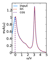
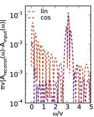
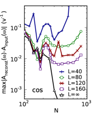
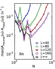
Figure 4: (Color online) Reconstruction of the spectral function of Fig. 1 represented by the discrete Hamiltonian (29). Top left: Input function and reconstructed functions using $L=80$, $N=200$, $a=100v$, $b=-0.995$. We compare the linear discretization (26) with the cosine (28) discretization. Top right: Difference of input and reconstructed functions of the top left panel. Bottom left: The error $\max_{\omega\geq 0}|A_{\text{reconst}}(\omega)-A_{\text{input}}(\omega)|$ versus number $N$ of computed Chebyshev moments using a cosine discretization. Bottom right: Error for linear discretization.

In Fig. 4, we show the reconstruction of spectral functions based on the linear prediction of the moments computed for $\widetilde{A}_{\text{discr}}^{>}(\omega)$ using the operator-valued Chebyshev expansion presented in Sec. I.2 for the “Hamiltonian” defined in (29). This is analogous to the top left panel of Fig. 3, which treated the thermodynamic limit.

For the finite-size system, the specific choice of discretization is important and we compare the linear and the cosine discretization in the top panels of Fig. 4 for the expansion order $N=200$ and a system size $L=80$. From the large error at $\omega=0$ for the linear discretization (red dashed line) seen in the right top panel of Fig. 4, which was not present in the thermodynamic limit (red dashed line in right top panel of Fig. 3), we conclude that the linear discretization starts resolving finite-size features close to $\omega=0$ already for $N=200$. The lower panels then show how the error behaves as a function of the number of computed moments for different system sizes $L$. While the cosine discretization follows the error of the thermodynamic limit quite closely for low values of $N$ and lattice sizes of $L\geq 80$, it almost saturates in a plateau for higher expansion orders, and only starts increasing slightly for very high expansion orders. For the linear discretization, neither the close correspondence with the thermodynamic limit is observed, nor does the error only moderately depend on the expansion order: Instead, the error increases exponentially for high values of $N$, as then, finite-size features are inhomogeneously resolved. Both features make it difficult to determine the value of $N$ for which the computation of Chebyshev moments should be stopped in order to obtain a minimal error.

IV Implications for MPS representations

What is the relevance of the previous results for matrix product state (MPS) based computations of the spectral function for a given matrix product operator (MPO) $H$?(Schollwöck, 2011) Repeated MPO operations on MPS create entanglement, which eventually makes manipulating and storing MPS computationally very costly. Manipulations, such as applying $H$ to states $|t_{n}\rangle$ in the recursion (13), or performing subsequent time evolution steps $e^{-iH\Delta t}$, can therefore only be carried out up to a certain recursion order $n$ or time $t$, before hitting an exponential wall in computation cost. For time evolution algorithms, this has long been known,(Gobert et al., 2005; Eisert and Osborne, 2006) but this also limits computations using the Chebyshev recursion.(Wolf et al., 2014a)

In the following, we show that the method introduced in the previous sections outperforms the previous approach:(Ganahl et al., 2014a) it extracts more spectral information from $H$ when creating the same amount of entanglement or, which is equivalent up to technical details of the algorithm, using the same computation time.

As an example, we compute the spectral function of the single impurity Anderson model (SIAM), which serves as a common benchmark(Raas et al., 2004; Ganahl et al., 2014a, b; Wolf et al., 2014a, b) and is highly relevant as it is at the core of dynamical mean-field theory (DMFT).(Metzner and Vollhardt, 1989; Georges and Kotliar, 1992; Georges et al., 1996; Kotliar et al., 2006)

The Hamiltonian of the SIAM is given as,

$$H^{\text{SIAM}} =H_{\text{imp}}+H_{\text{bath}}+H_{\text{hyb}},$$ (30)

$$H_{\text{imp}} =U\left(n_{0\uparrow}-\tfrac{1}{2}\right)\left(n_{0\downarrow}-\tfrac{1}{2}\right),$$

$$H_{\text{bath}} =\sum_{l=1}^{L_{b}}\sum_{\sigma}\epsilon_{l}c^{\dagger}_{l\sigma}c_{l\sigma},$$

$$H_{\text{hyb}} =\sum_{l=1}^{L_{b}}\sum_{\sigma}\left(V_{l}c^{\dagger}_{0\sigma}c_{l\sigma}+\text{H.c.}\right).$$

By a unitary transform effected by Lanczos tridiagonalization, this can be mapped on the so-called chain geometry. But as this leads to higher entanglement, we simply order bath states by their potential energy which directly gives a one-dimensional array that can be treated with MPS.(Wolf et al., 2014b) We solve the model for the semi-elliptic bath density of states

$$-\frac{1}{\pi}\text{Im}\Lambda(\omega)=\frac{1}{2v\pi}\sqrt{4-\Big{(}\frac{\omega}{v}\Big{)}^{2}},$$ (31)

which is discretized according to the procedure discussed in Sec. III, and then yields the parameters $\epsilon_{l}$ and $V_{l}$. It is important to realize that here, we discretize the bath hybridization function whereas in Sec. III, we discretized the spectral function. While Sec. III did this to illustrate the effect of discretization for a toy model for which the spectral function was known from the beginning, in the present case, a true many-body compuation is involved. In the present case, the relevant discretization parameter is the bath size $L_{b}=L-1$, and no longer the system size.(Wolf et al., 2014a)

We compute the spectral function (18) of the impurity Green’s function, where the initial states are single-particle excitations of the ground state: $|\psi_{0\sigma}^{>}\rangle=c_{0\sigma}^{\dagger}|E_{0}\rangle$ and $|\psi_{0\sigma}^{<}\rangle=c_{0\sigma}|E_{0}\rangle$. As we consider the particle-hole and spin-symmetric case of (30), we only need to compute one Chebyshev recursion; to be precise: $|\psi_{0}\rangle=c_{0\uparrow}^{\dagger}|E_{0}\rangle$. We compare our results with dynamic DMRG results from Ref. Raas et al., 2004, which are believed to be highly reliable. In particular, we compare computations in the formerly suggested setup(Holzner et al., 2011; Ganahl et al., 2014a) that uses the Chebyshev recursion for $b=0$ in (10) and reconstructs the full spectral function $A(\omega)$ using linear prediction,(Ganahl et al., 2014a) and the one suggested here, that uses $b=-0.995$ and reconstructs the shifted spectral function $\widetilde{A}(\omega)$ using linear prediction.

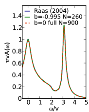
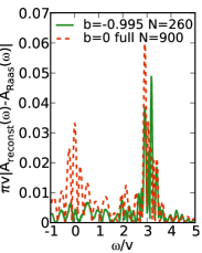
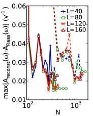
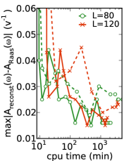
Figure 5: (Color online) Comparison of MPS computed spectral functions in the two setups studied in the previous sections, with data by Raas et al. (2004). Solid lines refer to the new method that uses $\widetilde{A}(\omega)$, dashed lines refer to the method that uses the full spectral function $A(\omega)$. Top left: For $L=80$ and two exemplary expansion orders. Top right: Errors of comparison in top left panel. Bottom left: Plot of the maximum error versus expansion order $N$. Bottom right: Plot of the maximum error versus computer time.

In the top left panel of Fig. 5, we show computations of the spectral function of the SIAM for $L=80$ for $N=260$ in the $b=-0.995$ setup, and $N=900$ in the $b=0$ setup and compare it with the result of Ref. Raas et al., 2004. We choose these two expansion orders, as they lead to a comparable maximum error, as shown in the top right panel of Fig. 5. In the $b=-0.995$ setup, this maximum error is slightly smaller. Around $\omega=0$, by contrast, the error in the $b=-0.995$ setup is much smaller. If we compare the computation time that is needed to reach this precision ($\text{max}|A_{\text{reconst}}(\omega)-A_{\text{input}}|\simeq 0.015/v$), we find that the $b=-0.995$ setup required $\sim$$145\text{\,}\mathrm{m}\mathrm{i}\mathrm{n}$ whereas the $b=0$ setup required $\sim$$434\text{\,}\mathrm{m}\mathrm{i}\mathrm{n}$. If one makes this comparison for a slightly larger error ($\text{max}|A_{\text{reconst}}(\omega)-A_{\text{input}}|\simeq 0.025/v$), realized for expansion order $N=120$ for the $b=-0.995$ setup, and for expansion order $N=200$ for the $b=0$ setup, the comparison in computation times reads $\sim$$12\text{\,}\mathrm{m}\mathrm{i}\mathrm{n}$ versus $\sim$$160\text{\,}\mathrm{m}\mathrm{i}\mathrm{n}$.

When studying the convergence of the maximum error with respect to expansion order $N$ in the lower left panel of Fig. 5, we see that this is, after a sharp decrease for low expansion orders, not monotonously decreasing. The previously mentioned choices, $N=260$ in the $b=-0.995$ setup and $N=900$ in the $b=0$ setup, both correspond to a minimum in the oscillations, as seen when inspecting the green solid (dashed) lines for the $b=-0.995$ ($b=0$) setup. The non-monotonicity makes general comparisons for the speedup difficult. But the lower right panel of Fig. 5 still shows that with only a few exceptions, the solid ($b=-0.995$) lines are always clearly below the dashed ($b=0$) lines. The logarithmic abscissa therefore indicates a high speedup.

V Comparison to time evolution

It is interesting to compare the efficiency of the available MPS algorithms to extract spectral information from $H$. Candidates are, aside from the dynamic DMRG,(Jeckelmann, 2002) which is believed to be computationally highly costly, time evolution and recursive algorithms. The latter are, in particular, expansions in Chebyshev polynomials(Holzner et al., 2011) and the Lanczos algorithm.(García et al., 2004; Dargel et al., 2012) Lanczos is numerical instable as the basis that it spans looses its orthogonality for high numbers of iterations.(Arbenz, 2012) This seems to to disqualify Lanczos as a high-performing candidate. Therefore the main question is whether the Chebyshev recursion can more efficiently extract spectral information from $H$ than time evolution algorithms.

To answer this question, in the following, we exploit the fact that for $b=0$ in the limit $a\rightarrow\infty$, the Chebyshev expansion becomes a Fourier expansion, and the Chebyshev states directly describe the time evolved system. This is different from the procedure of computing the time dependence of a Green’s function via a Fourier transform of its spectral function.(Tal-Ezer and Kosloff, 1984; Leforestier et al., 1991; Holzner et al., 2011; Halimeh. et al., 2015) For comparison, we summarize the latter technique in Appendix E.

The approximate equivalence of the Chebyshev recursion to time evolution can be used as a novel time evolution algorithm. This is interesting as for long-range interacting Hamiltonians $H$, the MPO representation of $e^{-iHt}$ is not available, or only approximately.(Zaletel et al., 2014) Although it is possible to use so-called Krylov algorithms for such problems, this requires some programming effort, and is in general believed to be numerically rather inefficient as compared ot other time evolution algorithms. Long-range interacting problems appear e.g. if mapping a two-dimensional system on a one-dimensional chain, or in the solution of a SIAM using a star geometry(Wolf et al., 2014b) as in (30).

V.1 Statement of approximate equivalence

The time evolution of a state $|\psi_{0}\rangle$

$$|\psi(t)\rangle=\exp(-iHt)|\psi_{0}\rangle,$$ (32)

can be approximately linked to the sequence of Chebyshev vectors generated by starting from $|\psi_{0}\rangle$ as follows.

Choose a reference energy $E_{\text{ref}}$ in (10) that is characteristic for the initial state of the time evolution and the Chebyshev recursion. When computing the time evolution of the Green’s function with $|\psi_{0}\rangle=c^{\dagger}|E_{0}\rangle$, one chooses $E_{\text{ref}}=E_{0}$, if $|\psi_{0}\rangle$ is not an eigenstate, we choose $E_{\text{ref}}=\langle\psi_{0}|H|\psi_{0}\rangle$.

Then define $|\phi(t)\rangle=\exp(iE_{\text{ref}}t)|\psi(t)\rangle$ and $\mathcal{H}=(H-E_{\text{ref}})/a$ as in (10) in the $b=0$ setup. Here $a$ has the meaning of an inverse time step of unit energy. With these definitions, (32) reads as

$$|\phi(t)\rangle =\exp(-ia\mathcal{H}t)|\psi_{0}\rangle$$

$$=\big{(}\cos(a\mathcal{H}t)-i\sin(a\mathcal{H}t)\big{)}|\psi_{0}\rangle$$

$$\equiv|\phi_{\text{cos}}(t)\rangle-i|\phi_{\text{sin}}(t)\rangle.$$ (33)

Let us discretize time by defining $t_{n}=\frac{n}{a}$, then

$$|\phi_{\text{cos}}(t_{n})\rangle=\cos(n\mathcal{H})|\psi_{0}\rangle,$$ (34a)

$$|\phi_{\text{sin}}(t_{n})\rangle=\sin(n\mathcal{H})|\psi_{0}\rangle.$$ (34b)

We now want to compute the action of $\cos(n\mathcal{H})|\psi_{0}\rangle$ on $|\psi_{0}\rangle$ using a recursion that only involves the action of $\mathcal{H}$. This is not possible with the standard recursion for the cosine function, as shown in Appendix F.1.

Let us instead consider the action of the Chebyshev polynomials

$$T_{n}(\mathcal{H})=\cos(n\arccos(\mathcal{H}))$$ (35)

on $|\psi_{0}\rangle$. This action approximately reproduces the action of the plane cosine function, if we consider every 4th iteration, i.e. introduce the new index $n^{\prime}=4n$, $n\in\mathbb{N}$:

$$T_{n^{\prime}}(\mathcal{H})|\psi_{0}\rangle =\cos\Big{(}n^{\prime}\Big{(}\frac{\pi}{2}-\mathcal{H}\Big{)}\Big{)}|\psi_{0}\rangle+\epsilon(n^{\prime})|\psi_{0}\rangle$$ (36)

$$=\cos\Big{(}n^{\prime}\mathcal{H}\Big{)}|\psi_{0}\rangle+\epsilon(n^{\prime})|\psi_{0}\rangle.~{}n^{\prime}=0,4,8,...$$

In the first line, we used the Taylor expansion $\arccos(\mathcal{H})=\frac{\pi}{2}-\mathcal{H}+\frac{1}{6}\mathcal{H}^{3}+\cdots$, that leads to the error function $\epsilon(n^{\prime})$ (Appendix F.5), and in the second line, we used $n^{\prime}\frac{\pi}{2}=2\pi n$, $n\in\mathbb{N}$, which obviously drops out of the argument of the cosine (also see Appendix F.2).

The error $\epsilon(n^{\prime})$ is bounded by (78)

$$|\epsilon(t_{n^{\prime}})| =\frac{t}{t_{\text{err}}}\qquad\text{if}\quad t<t_{\text{err}}$$

$$t_{\text{err}} =\frac{a^{2}}{\sigma^{3}}$$ (37)

where $\sigma$ is the spectral width of the initial state $|\psi_{0}\rangle\equiv|\psi_{0}\rangle$ around $E_{\text{ref}}$,

$$\sigma=\max_{|E_{k}\rangle\in|\psi_{0}\rangle}|E_{k}-E_{\text{ref}}|,$$ (38)

where “$|E_{k}\rangle\in|\psi_{0}\rangle$” refers to the decomposition of the initial state in eigenstates $|E_{k}\rangle$ of $\mathcal{H}$

$$|\psi_{0}\rangle=\sum_{k}c_{k}|E_{k}\rangle.$$ (39)

The “spectral width” $\sigma$ is usually small compared to reasonably high values of the inverse time step $a$. If one is unsure of whether $a$ was chosen large enough, one reruns a calculation with a higher value of $a$ and checks convergence.

We can now compute the time evolution

$$|\phi_{\text{cos}}(t_{n^{\prime}})\rangle =|\phi_{\text{cheb}}(t_{n^{\prime}})\rangle+\epsilon(t_{n^{\prime}})|\psi_{0}\rangle,$$

$$|\phi_{\text{cheb}}(t_{n^{\prime}})\rangle =T_{n^{\prime}}(\mathcal{H})|\psi_{0}\rangle,\quad n^{\prime}=0,4,8,\dots$$ (40)

via the recursion (13)

$$|\phi_{\text{cheb}}(t_{n})\rangle =2\mathcal{H}|\phi_{\text{cheb}}(t_{n-1})\rangle-|\phi_{\text{cheb}}(t_{n-2})\rangle,$$

$$|\phi_{\text{cheb}}(t_{1})\rangle =\mathcal{H}|\psi_{0}\rangle,\quad n=0,1,2,\dots.$$ (41)

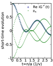
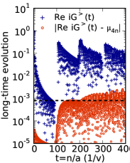
Figure 6: (Color online) Left: Time evolution of a particle created on the first site of a chain of length $L=100$ with hopping $v=1$ that is $|\psi_{0}\rangle=c_{0}^{\dagger}|\text{vac}\rangle$. We compare the time evolution of the Green’s function $iG^{>}(t)=e^{iE_{0}t}\langle\psi_{0}|\psi(t)\rangle$ (shown as blue crosses) with the Chebyshev moments $\mu_{n}=\langle\psi_{0}|\psi_{n}\rangle$ (shown as green dots) obtained when computing the recursion $|\psi_{n}\rangle=2H/a|\psi_{n-1}\rangle-|\psi_{n}-2\rangle$. Hopping amplitudes $v_{l}$ are obtained from the discretization of the spectral function of Fig. 1. A qualitatively equivalent behavior is obtained for a chain with homogeneous hopping $v_{l}=v$. Right: Long-time evolution of the Green’s function (blue crosses), and difference of the Green’s function and the Chebyshev moments (red dots). The horizontal dashed line marks the the prefactor of the error estimate (37), which is computed as $\sigma^{3}/a^{2}=8\cdot 10^{-4}$.

V.2 Numerical examples

V.2.1 Single-particle computation for SIAM

Fig. 6 shows the numerically exact time evolution of a single particle created on the first site $|\psi_{0}\rangle=c_{0}^{\dagger}|E_{0}\rangle$ of a chain of 100 lattice sites. The spectral width therefore is $\sigma=2v$. The left panel of Fig. 6 plots the Chebyshev moments $\mu_{n}=\langle\psi_{0}|t_{n}\rangle$ obtained with $a=100v$ and the time evolution of the corresponding Green’s function $iG^{>}(t)=e^{iE_{0}t}\langle\psi_{0}|\psi(t)\rangle$ for the time step $\frac{4}{a}$. Every forth Chebyshev moment agrees with a value of the Green’s function. In the right panel, we show the long time behavior of $G^{>}(t)$ and the difference $G^{>}(4n/a)-\mu_{4n}$. The difference is seen to be clearly below the conservative upper bound (37), it remains of the order of $\sigma^{3}/a^{2}=8\cdot 10^{-4}$ up to very high times that correspond to 100 hopping processes ($t=100/v$).

V.2.2 MPS computation for SIAM

We now study the time evolution of the SIAM (7) in the star geometry(Wolf et al., 2014b) for the single-particle excitation $|\psi_{0}\rangle=c_{0\uparrow}^{\dagger}|E_{0}\rangle$ of the half-filled ground state $|E_{0}\rangle$. The left panel shows the time evolution of the corresponding Green’s function, computed with an MPS Krylov algorithm that imposes the error bound

$$\big{|}\big{|}\,|\psi(t+\Delta t)\rangle-\exp(-iH\Delta t)|\psi(t)\rangle\,\big{|}\big{|}<\varepsilon_{\text{kry}},$$

for a time step of $\Delta t=\frac{4}{a}$. An error bound of $\varepsilon_{\text{kry}}=5\cdot 10^{-4}$ suffices to reliably compute times up to $15/v$.

In the MPS implementation of the Chebyshev recursion, we fix the global truncation error per iteration step, as discussed in Ref. Wolf et al., 2014a

$$\big{|}\big{|}\,|t_{n}\rangle-(2\mathcal{H}|t_{n-1}\rangle-|t_{n-2}\rangle)\,\big{|}\big{|}<\varepsilon_{\text{che}}.$$ (42)

To achieve this, two options are available. If during the variational compression of $(2\mathcal{H}|t_{n-1}\rangle-|t_{n-2}\rangle)$, the truncation error exceeds $\varepsilon_{\text{che}}$, even when choosing a better and better guess state, one can either directly increase the bond dimension, or reduce the truncated weight per bond, which indirectly increases the bond dimension. While for the setup in Ref. Wolf et al., 2014a, there were reasons to choose the former option, here we choose the latter as our Krylov algorithm uses a similar adaption.

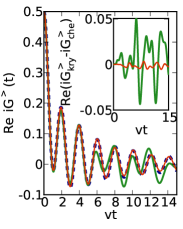
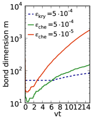
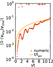
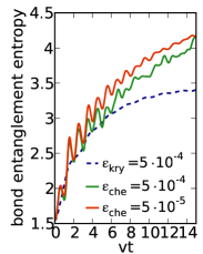
Figure 7: (Color online) Time evolution of the single particle excitation $c_{0\uparrow}^{\dagger}|E_{0}\rangle$ in the half-filled single impurity Anderson Model (30) with semi-elliptic density of states of half-bandwidth $2v$ and interaction $U/v=4$ for $L=40$. Computations using an MPS Krylov algorithm with error tolerance $\varepsilon_{\text{kry}}=5\cdot 10^{-4}$ and the Chebyshev recursion (40) for different error tolerances $\varepsilon_{\text{che}}=5\cdot 10^{-4}$ and $\varepsilon_{\text{che}}=5\cdot 10^{-5}$. Top left: Time evolution of Greens’s function. Both algorithms produce the same result upon using the smaller error tolerance for the Chebyshev algorithm. The legend is found in the top right panel. Top right: Maximal bond dimension, located at the central bond. The Krylov time evolution leads to a much smaller maximal bond dimension, as its computation produces a faithful result already with the relatively high error tolerance of $\varepsilon_{\text{kry}}=5\cdot 10^{-4}$, for which the Chebyshev algorithm shows strong errors in the Green’s function. Bottom left: Difference of overlap of Chebyshev and Krylov evolved states, comparing the $\varepsilon_{\text{che}}=5\cdot 10^{-5}$ with the $\varepsilon_{\text{kry}}=5\cdot 10^{-4}$ computation. The difference of overlap is bounded by the analytical prediction of (37), except for few exceptions that lie above it. These exceptions are of purely numerical origin as they are not visible in any other quantity. For the highest times shown, truncation errors have accumulated so much that the analytical prediction starts to fail. Bottom right: Bond entanglement entropy at center bond.

We compare the results of the Krylov algorithm with the Chebyshev algorithm (40). In the top left panel of Fig. 7, we plot the Green’s function $iG^{>}(t)=e^{iE_{0}t}\langle\psi_{0}|\psi(t)\rangle$. If imposing the same error tolerance $\varepsilon_{\text{che}}=\varepsilon_{\text{kry}}$, we obtain agreement of both algorithms only for short times. Only a much smaller tolerance for the Chebyshev algorithm $\varepsilon_{\text{che}}=\frac{1}{10}\varepsilon_{\text{kry}}$ leads to agreement also for long times. We conclude that error accumulation in the Chebyshev recursion is much worse conditioned than in the time evolution algorithm, and even worse than what could be expected from the four “auxiliary steps” made in (41) between each “physical time step”: imposing a tolerance $\varepsilon_{\text{che}}=\frac{1}{4}\varepsilon_{\text{kry}}$ for the Chebyshev recursion is not sufficient to produce comparable results.

The reduced error tolerance $\varepsilon_{\text{che}}=\frac{1}{10}\varepsilon_{\text{kry}}$ for the Chebyshev recursion comes at the price of an order of magnitude increase in the bond dimension compared to the Krylov algorithm, as shown in the top right panel of Fig. 7. But also for $\varepsilon_{\text{che}}=\varepsilon_{\text{kry}}$, the Chebyshev recursion needs higher bond dimensions than the Krylov algorithm. The lower left panel compares the overlap of the Chebyshev-evolved and the Krylov-evolved states by plotting $|1-\langle\psi_{\text{cheb}}|\psi_{\text{kry}}\rangle/\langle\psi_{\text{cheb}}|\psi_{\text{cheb}}\rangle|$. With only few exceptions, this quantity is bounded by the theoretical prediction of (37), when setting $\sigma=4v=U$. The exceptions are artifacts of the detailed implementation of the algorithms as the key observable $G^{>}(t)$ is correctly computed, but still their existence suggest that the implementation can be improved. Ignoring these exceptions, we see that the normalized overlap $\langle\psi_{\text{cheb}}|\psi_{\text{kry}}\rangle$ deviates from one only by a few percent even for long times. But these few percent come with a considerable growth of the entanglement entropy, as can be concluded by inspecting the lower right panel of Fig. 7. There, already the $\varepsilon_{\text{che}}=\varepsilon_{\text{kry}}$ case shows a considerably increased entropy.

Aside from the two preceding fundamental reasons (different error accumulation, small difference of states), the increased bond dimensions in the Chebyshev algorithm can also be related to a purely technical question: the variational compression(Schollwöck, 2011) in each Chebyshev iteration produces a state that fulfills (42), but might be a state with unnecessarily high bond dimension $m$. Similarly to the DMRG ground state optimization algorithm, also variational compression can get stuck in local minima. Currently, we use White’s mixing factor(White, 2005) to avoid this. A recent publication suggests an even better strategy and explains these problems concisely.(Hubig et al., 2015)

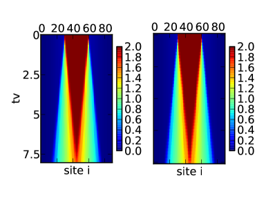
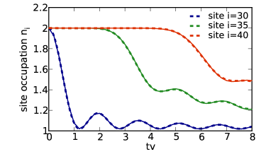
Figure 8: (Color online) Time evolution of a one dimensional fermionic Hubbard model on $L=90$ sites, with an interaction of $U/v=4$ and nearest neighbor hopping $v$ starting from a product state (double occupation in the center of the system). Left: Chebyshev computation using $\varepsilon_{\text{che}}=0.0001$. Right: Krylov computation using $\varepsilon_{\text{kry}}=\varepsilon_{\text{che}}$. Bottom: Detailed comparison for the occupation of specific sites. Chebyshev results are shown as dashed lines, Krylov results are shown as solid lines. Deviations are smaller than 1%.

In general the subspace of the Hilbert space that is needed to be faithfully described in order to measure the spectral function can be spanned using different basis states. In principle, the most efficient spanning would be provided by the Lanczos algorithm, as the latter provides orthogonal states. But it is impractical due to numerical instability. The basis states provided by time evolution or the Chebyshev recursion are not orthogonal to each other, but can be stably generated. The numerical evidence discussed in the previous paragraphs indicates that the Chebyshev recursion generates a much higher entangled basis of this subspace than a time evolution algorithm: it extracts less spectral information when fixing a maximal entanglement entropy. But these arguments directly hold only for the “$b=0$ setup” of the Chebyshev recursion, in which it is transparently comparable with a time evolution algorithm as there is a one-to-one correspondence of time evolution steps and iterations of the recursion.

Sections II–IV of this paper showed that the $b=0$ setup is the computationally least favorable setup of the Chebyshev recursion, and a $b\simeq-1$ setup much better. Still the gains in computation time of the $b\simeq-1$ setup over the $b=0$ setup shown in the bottom right panel of Fig. 5 seem not to be sufficient to compensate the clear inferiority of the Chebyshev method shown in the upper right panel of Fig. 7. A definitive statement is difficult due to the non-monotonic behavior of the error in Fig. 5 and due to the fact that such a comparison is strongly affected by the details of the implementation of the algorithms, and not only by the principle nature of how strongly entangled its resulting basis states are. For this reason, the discussion on the most efficient method for computing spectral functions using MPS cannot be generally considered settled.

V.2.3 Expansion in Hubbard model

Finally, we study the time evolution of the one-dimensional Hubbard model

$$H^{\text{Hubbard}}=U\sum_{l}\left(n_{l\uparrow}-\tfrac{1}{2}\right)\left(n_{l\downarrow}-\tfrac{1}{2}\right)$$

$$-v\sum_{l\sigma}(c^{\dagger}_{l\sigma}c_{l+1\sigma}+\text{h.c.}),$$ (43)

starting from a product state with doubly occupied sites in the center of the system, and evolving this state at interaction $U/v=4$, as shown in Fig. 8. We obtain very good agreement of the Krylov and the Chebyshev algorithm, although there is no rigorous a priori reason, for which the initial product state should have a narrow spectral width, i.e. small $\sigma$ in the sense of (38), as was the case for the single particle excited initial state. On the other hand, for example in the many studies on the eigenstate thermalization hypothesis(Deutsch, 1991; Srednicki, 1994) it is a frequently met assumption that for typical initial states the energy distribution around its mean value is extremely narrow, with a width of the order of the single-particle energy scale (see e.g. Ref. Rigol et al., 2007 Fig. 3b).

VI Conclusion

We started by linking linear prediction to analytic continuation, which explains why linear prediction is a reasonable method to extrapolate both Fourier and Chebyshev expansions of spectral functions. In order to apply linear prediction, we introduced a new method to avoid the algebraic convergence of Chebyshev moments (expansion coefficients) of generic step-like spectral functions. This amounts to a particular redefinition of the series expansion that is based on a subtraction of the Chebyshev moments of a self-consistently determined step function.

We then showed that this allows to reduce the expansion order by a factor $\frac{1}{6}$ as compared to the existing method.(Ganahl et al., 2014a) For linearly scaling algorithms, as in exact diagonalization,(Weiße et al., 2006; Lin et al., 2013) this means a reduction of computation time of the same factor. But also for matrix product state computations high speedups are obtained. Furthermore, we showed how to adapt the discretization of hybridization functions of impurity models to the Chebyshev method.

Finally, we showed the approximate equivalence of the Chebyshev recursion to time evolution in a certain limit. This lead to a novel time evolution algorithm and allowed to transparently compare standard time evolution and the Chebyshev recursion in how efficient they extract spectral information from an operator $H$. For exact representations, the Chebyshev recursion is superior to time evolution as the latter is equivalent to the least favorable setup of the Chebyshev expansion, which can be improved by the previously mentioned factor $\frac{1}{6}$. For matrix product state representations, our results indicate that the Chebyshev expansion is inferior: we observe a much higher entanglement production in the Chebyshev recursion than in standard time evolution. We identify as main reason for this an unfavorable error accumulation in the Chebyshev recursion that requires computations at higher accuracy. So while in the history of the solution of differential equations for non-time periodic problems, Chebyshev expansions replaced Fourier expansions in the course of time,(Boyd, 2001) in the matrix product state context such a transition now seems unlikely. Still the Chebyshev recursion provides an easy-to-implement and straight-forward way to compute spectral functions.

Relevant applications of the results of this paper are the computation of conductivities,(Garcia et al., 2014) the computation of time evolution of long-range interacting systems,(Zaletel et al., 2014) and in particular, the challenging solution of dynamical mean-field theory.(Ganahl et al., 2014a; Wolf et al., 2014a) For example, the latter can usually not be accessed by combining analytical and numeric techniques as recently done for the Hubbard model in Ref. Seabra et al., 2014.

VII Acknowledgements

FAW acknowledges fruitful discussions with D. Braak, M. Eckstein and R. Leike, and support by the research unit FOR 1807 of the DFG.

Appendix

Appendix A Convergence speed

Analogously to Ref. Boyd, 2001, Chap. 2.9, we give the argument for the speed of convergence of the Chebyshev sequence, computed with the non-weighted inner product of (6b)

$$\mu_{n} =\int_{-1}^{1}dxf(x)T_{n}(x)$$

$$=\int_{0}^{\pi}d\theta f(\cos\theta)\cos(n\theta)\sin\theta$$

$$=\text{Re}\int_{0}^{\pi}d\theta\widetilde{f}(\cos\theta)e^{in\theta},$$ (44)

where $\widetilde{f}(\theta)=f(\cos\theta)\sin\theta$. We can then do $k$ partial integrations, if $\widetilde{f}(\theta)$ is $k$ times differentiable

$$\mu_{n} =\text{Re}\Big{[}-\sum_{j=1}^{k}\Big{(}\Big{(}\frac{i}{n}\Big{)}^{j}e^{in\theta}\widetilde{f}^{(j-1)}(\theta)\Big{|}_{0}^{\pi}\Big{)}$$

$$\qquad+\Big{(}\frac{i}{n}\Big{)}^{k}\int_{0}^{\pi}d\theta\widetilde{f}^{(k)}(\theta)e^{in\theta}\Big{]},$$ (45)

where $\widetilde{f}^{(j)}(\theta)$ denotes the $j$th derivative of $\widetilde{f}(\theta)$. If $\widetilde{f}^{(j)}(0)=\widetilde{f}^{(j)}(\pi)=0$ for $j=0,\dots,k-1$, which is fulfilled for typical single-particle spectral functions as in Fig. 2, and if $\widetilde{f}^{(k)}(\theta)$ is integrable, (A) constitutes an upper bound $\mathcal{O}\big{(}\frac{1}{n^{k}}\big{)}$ for the sequence $\mu_{n}$.

Appendix B Examples for linear prediction of Chebyshev expansions

In Sec. II, we compared the reconstruction of a spectral functions using its extrapolated (linearly predicted) Chebyshev expansion. We focussed on a typical example for this discussion, given by the $U/v=4$ spectral function of the half-filled SIAM with semi-elliptic bath density of states, which is shown in the top panel of Fig. 1.

In this appendix, we support the arguments of Sec. II by showing further generic examples. Starting from a step-like input function $A^{>}(\omega)$, we again compare the two reconstructions based on (i) linearly predicting the “subtracted” spectral function $\widetilde{A}^{>}(\omega)$ of (17) and (ii) linearly predicting the “full” (summed particle and hole contributions) spectral function $A(\omega)$ of (18).

To consider generic cases, we study functions that show “features” at $\omega=0$ and at some distance, of order of the single-particle bandwidth, away from it. The most natural choice for constructing such functions are superpositions of (non-normalized) Lorentzians and Gaussians

$$f^{>}(\omega) =\left\{\begin{array}[]{ll}0&\text{for }\omega<0\\ \sum_{\omega_{0}\in\{0,4\}}h(\omega,\omega_{0})&\text{else,}\end{array}\right.$$ (48)

$$h_{l}(\omega,\omega_{0}) =\frac{\eta^{2}}{(\omega-\omega_{0})^{2}+\eta^{2}},$$

$$h_{g}(\omega,\omega_{0}) =e^{-\frac{(\omega-\omega_{0})^{2}}{2\eta^{2}}}.$$

The function $f^{>}(\omega)$ is plotted for both choices in the top panels of Figs. 9 and 10 for $\eta=0.2$.

Based on the same argument as is the basis for Sec. V in this paper (approximate equivalence of Fourier and Chebyshev expansion), Ref. Wolf et al., 2014a showed the decrease of Chebyshev moments for superpositions of Lorentzians and Gaussians, to be approximately exponential and $\propto e^{-\alpha n^{2}}$, respectively. This behavior is observed in both center panels of Figs. 9 and 10. For high values of $n$, in Fig. 10, the decrease $\propto e^{-\alpha n^{2}}$ transitions into an exponential decrease, which is not in contradiction with the result of Ref. Wolf et al., 2014a. This, as the discussion of Sec. V, make statements for intermediate values of $n$.

In the bottom panels of Figs. 9 and 10 we then show the error obtained for the different methods of reconstruction. Linearly predicting $\widetilde{A}^{>}(\omega)$ yields considerably lower errors than linearly predicting the “full” spectral function $A(\omega)$. Only in the case of Lorentzians (lower panel of Fig. 9), using $A(\omega)$ leads to lower errors for values of $n$.

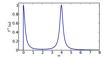
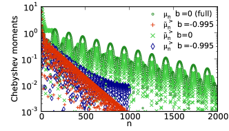
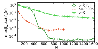
Figure 9: (Color online) Top: Test function consisting of two Lorentzians (48). Center: Corresponding Chebyshev moments in the three different setups $\mu^{>}$, $\widetilde{\mu}^{>}$ and $\mu$, analogously to the bottom panel of Fig. 2. Bottom: Error of reconstructed spectral function, analogously to the bottom panel of Fig. 3. All of this is for $a=100$.

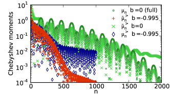
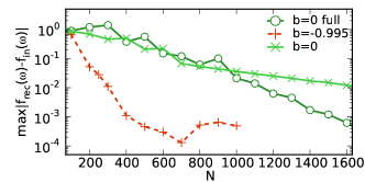
Figure 10: (Color online) Top: Test function consisting of two Gaussians (48). Center: Corresponding Chebyshev moments in the three different setups $\mu^{>}$, $\widetilde{\mu}^{>}$ and $\mu$, analogously to the bottom panel of Fig. 2. Bottom: Error of reconstructed spectral function, analogously to the bottom panel of Fig. 3. All of this is for $a=100$.

Finally, in Fig. 11, we show results for the spectral function of the half-filled non-interacting SIAM with semi-elliptic bath density of states, which itself is semi-elliptic,

$$A^{>}(\omega)=\left\{\begin{array}[]{ll}\qquad 0&\text{for }\omega<0,\\ \qquad 0&\text{for }\omega>2v,\\ \frac{1}{2v\pi}\sqrt{4-\Big{(}\frac{\omega}{v}\Big{)}^{2}}&\text{else.}\end{array}\right.$$ (52)

$A^{>}(\omega)$ has a kink at $\omega=2v$, as can be seen in the top panel of Fig. 11. Therefore, Chebyshev moments decrease only algebraically, as seen in the center panel of Fig. 11.

If we consider the error of the linear-prediction-based reconstructed $A^{>}(\omega)$, shown in the bottom panel of Fig. 11, we see that this yields much better results than the estimate (21) gives for a plain truncation of an algebraically decreasing series. Concerning the comparison between the two methods of reconstructing $\widetilde{A}^{>}(\omega)$ and the full $A(\omega)$, we observe that $\widetilde{A}^{>}(\omega)$ yields to smaller errors throughout.

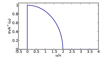
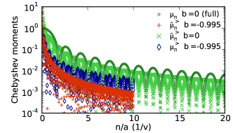
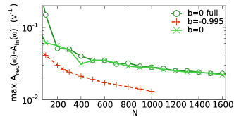
Figure 11: (Color online) Top: Particle spectral function of half-filled non-interacting SIAM. Center: Corresponding Chebyshev moments in the three different setups $\mu^{>}$, $\widetilde{\mu}^{>}$ and $\mu$, analogously to the bottom panel of Fig. 2. Bottom: Error of reconstructed spectral function, analogously to the bottom panel of Fig. 3.

We finally note that studying the spectral function of the non-interacting SIAM with a constant bath density of states as in Ref. Holzner et al., 2011 and Ref. Ganahl et al., 2014a, does not constitute a more general case. The analytic expression for this is very close to a single Lorentzian.

Appendix C Linear prediction

In the context of time evolution linear prediction has been long established in the DMRG community,(White and Affleck, 2008; Barthel et al., 2009) but it has only recently been applied to the computation of Chebyshev moments.(Ganahl et al., 2014a; Wolf et al., 2014a) The optimization problem for the sequence $\mu_{n}$ becomes linear, if the sequence can be defined recursively

$$\tilde{\mu}_{n}=-\sum_{i=1}^{p}a_{i}\mu_{n-i},$$ (53)

which is easily found to be equivalent to (1).(Barthel et al., 2009) The strategy is then as follows. Compute $N_{c}$ Chebyshev moments, and predict moments for higher values of $n$ using (53).

The coefficients $a_{i}$ are optimized by minimizing the least-square error $\sum_{n\in\mathcal{N}_{\text{fit}}}|\tilde{\mu}_{n}-\mu_{n}|^{2}$ for a subset $\mathcal{N}_{\text{fit}}=\{N_{c}-n_{\text{fit}},\dots,N_{c}-1,N_{c}\}$ of the computed data. We confirmed $n_{\text{fit}}=N_{c}/4$ to be a robust choice, (i) small enough to go beyond complicated low-order (short-time) behavior and (ii) large enough to have a good statistics for the fit. Earlier,(Wolf et al., 2014a) we chose $n_{\text{fit}}=N_{c}/2$, which leads to a better statistics for the fit. But this improvement is not important, as we do not deal with stochastic data. Minimization yields

$$R\bm{a} =-\bm{r},\quad\bm{a}=-R^{-1}\bm{r},$$ (54)

$$R_{ji} =\sum_{n\in\mathcal{N}_{\text{fit}}}\mu^{*}_{n-j}\mu_{n-i},\quad r_{j}=\sum_{n\in\mathcal{N}_{\text{fit}}}\mu^{*}_{n-j}\mu_{n}.$$

Linear prediction is more prone to overfitting if choosing $p$ to be very high. Therefore one should restrict the number of coefficients to $p=\min(n_{\text{fit}}/2,100)$. Furthermore, one adds a small constant $\delta=10^{-6}$ to the diagonal of $R$ in order to enable the inversion of the singular matrix $R$. Defining(Barthel et al., 2009)

$$M=\left(\begin{array}[]{ccccc}-a_{1}&-a_{2}&-a_{3}&\dots&-a_{p}\\ 1&0&0&\dots&0\\ 0&1&0&\dots&0\\ \vdots&\ddots&\ddots&\ddots&\vdots\\ 0&0&\dots&1&0\\ \end{array}\right),$$

one obtains the predicted moments $\tilde{\mu}_{N_{c}+n}=(M^{n}\bm{\mu}_{N_{c}})$, where $\bm{\mu}_{N_{c}}=(\mu_{N_{c}-1}\;\mu_{N_{c}-2}\;\dots\;\mu_{N_{c}-p})^{T}$. The matrix $M$ might have eigenvalues with absolute value larger than $1$, either due to numerical inaccuracies or due to the fact that linear prediction cannot be applied as $\mu_{n}$ rather increases than decreases on the training subset $\mathcal{N}_{\text{fit}}$. In order to obtain a convergent prediction, we set the weights that correspond to these eigenvalues to zero measuring the ratio of the associated discarded weight compared to the total weight. If this ratio is higher than a few percent, we conclude that linear prediction cannot be applied. One can then restart the computation to increase the number of computed moments $N_{c}$, and try applying linear prediction for a higher number of moments.

Appendix D Discretization for odd $L$

In the case of odd $L$ we cannot equate the central interval boundary with 0 as in (27). Instead we have to choose the correct width for the “central interval” by choosing the neighboring boundaries $\omega_{(L+1)/2}$ and $\omega_{(L+1)/2+1}$ correctly. This is achieved by subtracting an offset $\Delta w$ from each of the positive boundaries defined in (28), such that for $l=1,2,...$

$$\omega_{(L+1)/2+l} =a\big{(}\cos(\theta_{(L+1)/2+1}+l\Delta\theta)-b-\Delta\omega\big{)},$$

$$\Delta\theta =\tfrac{2}{L}(\theta_{L+1}-\theta_{(L+1)/2+1}),$$

$$\theta_{(L+1)/2+1} =\arccos b,$$

$$\theta_{L+1} =\arccos(b+\tfrac{\omega_{L+1}}{a}),$$ (55)

$$\Delta\omega =\frac{1}{2}\big{(}\cos(\theta_{(L+1)/2+1}+\Delta\theta)-b\big{)}.$$

For negative boundaries $\Delta\omega$ has to be added instead of subtracted.

Appendix E Time evolution by Fourier transform

Given the Chebyshev expansion in frequency space

$$A^{>}(\omega) =\frac{1}{a}\mathcal{A}^{>}\big{(}\frac{\omega}{a}+b\big{)},$$

$$\mathcal{A}^{>}(x) =\sum_{n}w_{n}(x)\mu_{n}T_{n}(x),$$ (56)

we can obtain the time evolution of a single Green function, but not for the whole system state, by Fourier transforming

$$G^{>}(t) =\int_{-\infty}^{\infty}d\omega\,A^{>}(\omega)e^{i\omega t}$$

$$=\frac{1}{a}\int_{-\infty}^{\infty}d\omega\,\mathcal{A}^{>}\big{(}\frac{\omega}{a}+b\big{)}e^{i\omega t}$$

$$=\int_{-\infty}^{\infty}dx\,\mathcal{A}^{>}(x)e^{ia(x-b)t}$$

$$=\int_{-\infty}^{\infty}dx\,\sum_{n}w_{n}(x)\mu_{n}T_{n}(x)e^{ia(x-b)t}$$

$$=\sum_{n}\mu_{n}\int_{-\infty}^{\infty}dx\,w_{n}(x)T_{n}(x)e^{ia(x-b)t}$$

$$=e^{-iabt}\sum_{n}(2-\delta_{n0})(-i)^{n}\mu_{n}J_{n}(at),$$ (57)

where the last step (interchanging sum and integral) is only possible if the sum is absolutely convergent, or finite. The Fourier transform can be looked up in a handbook on integrals

$$\int_{-\infty}^{\infty}dx\, w_{n}(x)T_{n}(x)e^{ia(x-b)t}$$

$$=(2-\delta_{n0})e^{-iabt}\int_{-\infty}^{\infty}dx\,\frac{T_{n}(x)e^{iaxt}}{\pi\sqrt{1-x^{2}}}$$

$$=(-i)^{n}(2-\delta_{n0})e^{-iabt}J_{n}(at).$$ (58)

Appendix F Comparison to time evolution

F.1 Standard recursion for cosine

As usual for a vector space of orthogonal polynomials, the space of cosine functions $\{\cos(nx)\}$, where $n\in\mathbb{N},~{}x\in\mathbb{R}$, can be generated using a three-term recursion formula

$$\cos(nx)=2\cos(x)\cos((n-1)x)-\cos((n-2)x),$$ (59)

which can be proven using addition theorems.

Rewriting this in the operator-valued form for the argument $\mathcal{H}$, and acting on $|\psi_{0}\rangle$ yields for the definition of $|\phi_{\text{cos}}(t_{n})\rangle$ in Eq. (34)

$$|\phi_{\text{cos}}(t_{n})\rangle=2\cos\mathcal{H}|\phi_{\text{cos}}(t_{n-1})\rangle-|\phi_{\text{cos}}(t_{n-2})\rangle.$$ (60)

But this provides no solution for our problem as the action of $\cos\mathcal{H}$ on $|\phi_{\text{cos}}(t_{n-1})\rangle$ is not known.

F.2 Shifted cosine

Using an addition theorem

$$\cos\big{(}n (\tfrac{\pi}{2}-\alpha)\big{)}=$$ (61)

$$= \cos\big{(}n\tfrac{\pi}{2}\big{)}\cos(n\alpha)+\sin\big{(}n\tfrac{\pi}{2}\big{)}\sin(n\alpha)$$

$$= \left\{\begin{array}[]{cl}\cos(n\alpha)&\text{ if }\frac{n}{4}\in\mathbb{N}\\ \sin(n\alpha)&\text{ if }\frac{n+2}{4}\in\mathbb{N}\\ \frac{1}{\sqrt{2}}\big{(}\cos(n\alpha)+\sin(n\alpha)\big{)}&\text{ else.}\\ \end{array}\right.$$ (65)

Eq. (36) follows if setting $\alpha=\mathcal{H}$.

F.3 Sine term

Changing the initial conditions of (66a) generates the polynomials $T_{n}^{\prime}=\sin(n\arccos(x))$

$$T_{n}^{\prime}(x)=2xT_{n-1}^{\prime}(x)-T_{n-2}^{\prime}(x),$$ (66a)

$$T_{1}^{\prime}(x)=\sqrt{1-x^{2}},\quad T_{0}^{\prime}(x)=0,$$ (66b)

which approximates the sine function, in the same way as (36) approximates the cosine

$$T_{n}^{\prime}(\mathcal{H})\simeq\sin\Big{(}n\mathcal{H}\Big{)} \text{ if }n/4\in\mathbb{N}.$$ (67)

F.4 Bound for Arccos

Bounding the Arccos works as follows

$$\arccos(x) =\frac{\pi}{2}-\sum_{n=0}^{\infty}\frac{\binom{2n}{n}x^{2n+1}}{4^{n}(2n+1)}$$

$$=\frac{\pi}{2}-x-r(x)$$

$$r(x) =x^{3}\Big{(}\frac{1}{6}+\Big{|}\sum_{n=2}^{\infty}\frac{\binom{2n}{n}x^{2n-2}}{4^{n}(2n+1)}\Big{|}\Big{)}.$$ (68)

Using $\arcsin(1)=\sum_{n=0}^{\infty}\frac{\binom{2n}{n}}{4^{n}(2n+1)}=\frac{\pi}{2}$ we can bound

$$\left|r(x)\right| =|x^{3}|\Big{(}\frac{1}{6}+\Big{|}\sum_{n=2}^{\infty}\frac{\binom{2n}{n}x^{2n-2}}{4^{n}(2n+1)}\Big{|}\Big{)}$$

$$<|x^{3}|\Big{(}\frac{1}{6}+\Big{|}\sum_{n=2}^{\infty}\frac{\binom{2n}{n}}{4^{n}(2n+1)}\Big{|}\Big{)}$$

$$=|x^{3}|\Big{(}\frac{1}{6}+\frac{\pi}{2}-1-\frac{1}{6}\Big{)}$$

$$=|x^{3}|\Big{(}\frac{\pi}{2}-1\Big{)}$$

$$<\frac{2}{3}|x^{3}|.$$ (69)

F.5 Error computation

The approximation in (36) is based on the Taylor expansion

$$\arccos(\mathcal{H}) =\frac{\pi}{2}-\mathcal{H}+\frac{1}{6}\mathcal{H}^{3}+\mathcal{O}(\mathcal{H}^{5}),$$ (70)

$$\mathcal{H} =\frac{H-E_{\text{ref}}}{a},$$

which reflects the fact that the arcus cosine is well approximated already by the leading linear term around $x=0$.

The approximation of $|\phi(t_{n})\rangle$ that has been generated in this way, is good if $a$ is large enough and becomes exact for $a\rightarrow\infty$. But how large does one have to choose $a$ in practice in order for $\epsilon(t_{n^{\prime}})$ to be bounded by the wished accuracy?

Consider the decomposition of the initial state in eigen states $|E_{n}\rangle$ of $\mathcal{H}$

$$|\psi_{0}\rangle=\sum_{k}c_{k}|E_{k}\rangle,$$ (71)

and, defining $\omega_{k}=\frac{E_{k}-E_{\text{ref}}}{a}$, therefore

$$T_{n}(\mathcal{H})|\psi_{0}\rangle=\sum_{k}c_{k}T_{n}(\omega_{k})|E_{k}\rangle.$$ (72)

We are now only interested in indices $n^{\prime}$ that are multiples of $4n$, as only those have the interpretation of a time-evolved state. Therefore,

$$T_{n^{\prime}}(\omega_{k})= \cos(n^{\prime}\arccos(\omega_{k}))$$

$$= \cos(n^{\prime}\omega_{k}-n^{\prime}r_{k})\qquad\text{ as }n^{\prime}=4n,\,\text{see Eq.}\,\eqref{shiftCos}$$

$$= \cos(n^{\prime}\omega_{k})\cos(n^{\prime}r_{k})+\sin(n^{\prime}\omega_{k})\sin(mr_{k})$$

$$= \cos(n^{\prime}\omega_{k})+\epsilon_{k}(n^{\prime}),$$

$$\epsilon_{k}(n^{\prime}) =\cos(n^{\prime}\omega_{k})(\cos(mr_{k})-1)$$

$$\qquad+\sin(n^{\prime}\omega_{k})\sin(mr_{k})$$

Up to here everything was exact.

Now we can strictly bound the absolute value of the error term using $|\sin(r_{k})|<|r_{k}|$ and $|\cos(r_{k})-1|<\frac{r_{k}^{2}}{2}$ and trivially bounding $\cos(n^{\prime}\omega_{k})$ and $\sin(n^{\prime}\omega_{k})$ by one,

$$|\epsilon_{k}(n^{\prime})|<\tfrac{1}{2}n^{\prime 2}r_{k}^{2}+n^{\prime}|r_{k}|$$ (73)

Let us now define the energy eigenvector $|E_{\text{max}}\rangle$ for which the error $\epsilon_{k}$ becomes maximal, which is the one for which $\omega_{\text{max}}$ is maximal, i.e.

$$\omega_{\text{max}}=\max_{|E_{k}\rangle\in|\psi_{0}\rangle}\omega_{k}$$ (74)

with which we compute $r_{\text{max}}$ and $\epsilon_{\text{max}}$. We can then simplify further

$$\sum_{k}c_{k}\epsilon_{k}(n^{\prime})|E_{k}\rangle<\epsilon_{\text{max}}(n^{\prime})\sum_{k}c_{k}|E_{k}\rangle=\epsilon_{\text{max}}(n^{\prime})|\psi_{0}\rangle.$$

We therefore arrive at

$$T_{n^{\prime}}(\mathcal{H})|\psi_{0}\rangle=\cos(n^{\prime}\mathcal{H})|\psi_{0}\rangle+\epsilon(n^{\prime})|\psi_{0}\rangle$$ (75)

The value of $\omega_{\text{max}}$ is determined by the cutoff of the distribution of eigenvectors $|E_{k}\rangle$ in $|\psi_{0}\rangle$. This can be a strict cutoff or a few standard deviations of Gaussian distribution, beyond which no contributions with numerically measurable weight occur. Let denote this cutoff or width $\sigma$ and define it analogously to $\omega_{\text{max}}$, i.e.

$$\sigma=\max_{|E_{k}\rangle\in|\psi_{0}\rangle}|E_{k}-E_{\text{ref}}|\quad\Rightarrow\quad\omega_{\text{max}}=\frac{\sigma}{a}$$ (76)

If, e.g., $|\psi_{0}\rangle$ is constructed by applying a single-particle operator to an eigenstate (e.g. the ground state) of $H$, $\sigma$ is the single particle bandwidth $W_{\text{single}}$ times a small factor of order 1.

Finally we need to bound the error term $r_{k}$ (Appendix F.4)

$$r_{k}=\frac{1}{6}\omega_{k}^{3}+\mathcal{O}(\omega_{k}^{5}),\quad\left|r_{k}\right|<\frac{2}{3}|\omega_{k}^{3}|.$$ (77)

Using the definition of $\sigma$, let us now bound $\epsilon(n^{\prime})$

$$|\epsilon(n^{\prime})| <|\epsilon_{\text{max}}(n^{\prime})|$$

$$<\tfrac{1}{2}n^{\prime 2}r_{\text{max}}^{2}+n^{\prime}|r_{\text{max}}|$$

$$<\tfrac{1}{2}n^{\prime 2}(\tfrac{2}{3})^{2}\omega_{\text{max}}^{6}+n^{\prime}\frac{2}{3}|\omega_{\text{max}}^{3}|$$

$$=\tfrac{1}{2}n^{\prime 2}(\tfrac{2}{3})^{2}\Big{(}\frac{\sigma}{a}\Big{)}^{6}+n^{\prime}\frac{2}{3}\Big{(}\frac{\sigma}{a}\Big{)}^{3}$$

$$<\frac{3}{2}n^{\prime}\frac{2}{3}\Big{(}\frac{\sigma}{a}\Big{)}^{3}\qquad\text{if}\quad n^{\prime}<n^{\prime}_{\text{ref}}$$

$$=\frac{n^{\prime}}{n^{\prime}_{\text{ref}}},\quad n^{\prime}_{\text{ref}}=\Big{(}\frac{a}{\sigma}\Big{)}^{3}.$$

Or expressing this in units of time

$$|\epsilon(t_{n^{\prime}})| =\frac{t}{t_{\text{err}}}\qquad\text{if}\quad t<t_{\text{err}}$$

$$t_{\text{err}} =\frac{a^{2}}{\sigma^{3}}$$ (78)

Inserting typical values, where $v$ is a hopping energy for a single particle process: $\sigma=2v$, $a=100v$ one finds $t_{\text{err}}=\frac{1250}{v}$. The accumulated error $\epsilon(t_{n^{\prime}})$ therefore remains smaller than $10^{-2}$ if $t<12.5\frac{1}{v}$.

References

- Weiße et al. (2006) A. Weiße, G. Wellein, A. Alvermann, and H. Fehske, Rev. Mod. Phys. 78, 275 (2006).
- Gautschi (1967) W. Gautschi, SIAM Review 9, 24 (1967).
- Gautschi (1968) W. Gautschi, Mathematics of Computation 22, 251 (1968).
- Gautschi (1970) W. Gautschi, Mathematics of Computation 24, 245 (1970).
- Sack and Donovan (1971) R. A. Sack and A. F. Donovan, Numerische Mathematik 18, 465 (1971).
- Silver and Röder (1994) R. N. Silver and H. Röder, International Journal of Modern Physics C 05, 735 (1994).
- Wang (1994) L.-W. Wang, Phys. Rev. B 49, 10154 (1994).
- Wang and Zunger (1994) L.-W. Wang and A. Zunger, Physical Review Letters 73, 1039 (1994).
- Lin et al. (2013) L. Lin, Y. Saad, and C. Yang, (2013), arXiv:1308.5467 .
- Press et al. (2007) W. H. Press, S. A. Teukolsky, W. T. Vetterling, and B. P. Flannery, Numerical Recipes 3rd Edition: The Art of Scientific Computing, 3rd ed. (Cambridge University Press, New York, NY, USA, 2007).
- White and Affleck (2008) S. R. White and I. Affleck, Phys. Rev. B 77, 134437 (2008).
- Barthel et al. (2009) T. Barthel, U. Schollwöck, and S. R. White, Phys. Rev. B 79, 245101 (2009).
- Ganahl et al. (2014a) M. Ganahl, P. Thunström, F. Verstraete, K. Held, and H. G. Evertz, Phys. Rev. B 90, 045144 (2014a).
- Wolf et al. (2014a) F. A. Wolf, I. P. McCulloch, O. Parcollet, and U. Schollwöck, Phys. Rev. B 90, 115124 (2014a).
- Boyd (2001) J. B. Boyd, Chebyshev and Fourier Spectral Methods (Dover Publications, Mineola, New York, 2001).
- Raas et al. (2004) C. Raas, G. S. Uhrig, and F. B. Anders, Phys. Rev. B 69, 041102 (2004).
- Holzner et al. (2011) A. Holzner, A. Weichselbaum, I. P. McCulloch, U. Schollwöck, and J. von Delft, Phys. Rev. B 83, 195115 (2011).
- Bulla et al. (2008) R. Bulla, T. Costi, and T. Pruschke, Rev. Mod. Phys. 80, 395 (2008).
- Schollwöck (2011) U. Schollwöck, Annals of Physics 326, 96 (2011).
- Gobert et al. (2005) D. Gobert, C. Kollath, U. Schollwöck, and G. Schütz, Phys. Rev. E 71, 036102 (2005).
- Eisert and Osborne (2006) J. Eisert and T. Osborne, Physical Review Letters 97, 150404 (2006).
- Ganahl et al. (2014b) M. Ganahl, M. Aichhorn, P. Thunström, K. Held, H. G. Evertz, and F. Verstraete, preprint (2014b), arXiv:1405.6728 .
- Wolf et al. (2014b) F. A. Wolf, I. P. McCulloch, and U. Schollwöck, Phys. Rev. B 90, 235131 (2014b), arXiv:1410.3342 .
- Metzner and Vollhardt (1989) W. Metzner and D. Vollhardt, Physical Review Letters 62, 324 (1989).
- Georges and Kotliar (1992) A. Georges and G. Kotliar, Phys. Rev. B 45, 6479 (1992).
- Georges et al. (1996) A. Georges, G. Kotliar, W. Krauth, and M. J. Rozenberg, Rev. Mod. Phys. 68, 13 (1996).
- Kotliar et al. (2006) G. Kotliar, S. Savrasov, K. Haule, V. Oudovenko, O. Parcollet, and C. Marianetti, Reviews of Modern Physics 78, 865 (2006).
- Jeckelmann (2002) E. Jeckelmann, Physical Review B 66, 045114 (2002).
- García et al. (2004) D. J. García, K. Hallberg, and M. J. Rozenberg, Phys. Rev. Lett. 93, 246403 (2004).
- Dargel et al. (2012) P. E. Dargel, A. Wöllert, A. Honecker, I. P. McCulloch, U. Schollwöck, and T. Pruschke, Phys. Rev. B 85, 205119 (2012).
- Arbenz (2012) P. Arbenz, Numerical Methods for Solving Large Scale Eigenvalue Problems (Lecture Notes - ETH Zürich, 2012).
- Tal-Ezer and Kosloff (1984) H. Tal-Ezer and R. Kosloff, The Journal of Chemical Physics 81, 3967 (1984).
- Leforestier et al. (1991) C. Leforestier, R. Bisseling, C. Cerjan, M. Feit, R. Friesner, A. Guldberg, A. Hammerich, G. Jolicard, W. Karrlein, H.-D. Meyer, and et al., Journal of Computational Physics 94, 59 (1991).
- Halimeh. et al. (2015) J. C. Halimeh., F. Kolley, I. P. McCulloch, and U. Schollwöck, to be submitted to Phys. Rev. B (2015).
- Zaletel et al. (2014) M. P. Zaletel, R. S. K. Mong, C. Karrasch, J. E. Moore, and F. Pollmann, preprint (2014), arXiv:1407.1832 .
- White (2005) S. R. White, Phys. Rev. B 72, 180403 (2005).
- Hubig et al. (2015) C. Hubig, I. P. McCulloch, U. Schollwöck, and F. A. Wolf, (2015), arXiv:1501.05504 .
- Deutsch (1991) J. M. Deutsch, Phys. Rev. A 43, 2046 (1991).
- Srednicki (1994) M. Srednicki, Phys Rev E 50, 888 (1994), arXiv:cond-mat/9403051 .
- Rigol et al. (2007) M. Rigol, V. Dunjko, and M. Olshanii, Nature 452, 854 (2007), arXiv:0708.1324 .
- Garcia et al. (2014) J. H. Garcia, L. Covaci, and T. G. Rappoport, (2014), arXiv:1410.8140 .
- Seabra et al. (2014) L. Seabra, F. H. L. Essler, F. Pollmann, I. Schneider, and T. Veness, Phys. Rev. B 90, 245127 (2014), arXiv:1410.1670 .