Stability of Thin-Shell Wormholes from Noncommutative BTZ Black Hole

Abstract

In this paper, we construct thin-shell wormholes in (2+1)-dimensions from noncommutative BTZ black hole by applying the cut-and-paste procedure implemented by Visser. We calculate the surface stresses localized at the wormhole throat by using the Darmois-Israel formalism, and we find that the wormholes are supported by matter violating the energy conditions. In order to explore the dynamical analysis of the wormhole throat, we consider that the matter at the shell is supported by dark energy equation of state $p=\omega\rho$ with $\omega<0$. The stability analysis is carried out of these wormholes to linearized spherically symmetric perturbations around static solutions. Preserving the symmetry we also consider the linearized radial perturbation around static solution to investigate the stability of wormholes which explored by the parameter $\beta$ (speed of sound).

I Introduction

Wormholes and thin-shell wormholes are very interesting topic to the researcher for last two decades. Historically the concept of wormholes was first suggested by Flamm Flamm by means of the standard embedding diagram. After nineteen years a similar construction (wormhole type solution) attempted by Einstein’s and Rosen (1935) Einstein and Rosen known as ‘Einstein-Rosen Bridge’. They tried to investigate the fundamental particles like electrons as space-tunnels threaten by electric lines of force rather than to promote inter-universe travel. But these types of wormholes were not traversable. Interest in traversable wormholes, as a hypothetical shortcuts in space-time after introduced by Morris and Thorne MT1988 . Such types of wormholes are both traversable and stable as a solution of Einstein’s field equations having two asymptotically flat regions (same universe or may be two separate universe) connected by a minimal surface area, called throat, satisfying the flare-out condition HV1997 . Traversable wormholes have some issues such as the violations of energy conditions Visser 1995 ; Visser 2002 , the mechanical stability etc. which also stimulate researcher in several branches.

Though, it is very difficult to deal with the exotic matter (matter not fulfilling the energy conditions), Poisson and Visser Poisson constructed a thin-shell wormhole by cutting and pasting two identical copies of the Schwarzschild solution at $a>2M$, to form a geodesically complete new one with a shell placed in the joining surface. This construction restricts exotic matter to be placed at the wormhole throat and consider linearized radial perturbation around a static solution, in the spirit of Brady ; Balbinot for the stability of wormholes. Though the region of stability lies in a unexpected patch due to the lack of knowledge of known equations of state of exotic matter. Therefore, it is perhaps important to investigate the stability of static wormhole solutions by using specific equation of state (EoS) or by considering a linearized radial perturbations around a static solution. The choice of equation of state for the description of matter violating energy conditions present in the wormhole throat has a great relevance in the existence and stability of wormhole static solutions. Several models for the matter leading to such situation have been proposed Sahni ; Peebles ; Padmanabhan : one of them is the ‘dark energy’ models are parameterized by an equation of state w = p/$\rho$ where p is the spatially homogeneous pressure and $\rho$ is the dark energy density. A specific form of dark energy, denoted phantom energy, possessing with the peculiar property of w $<$ -1. As the phantom energy equation of state, p = w$\rho$ with $w<-1$, is now a fundamental importance to investigate the stability of these phantom thin-shell wormholes have been studied in Jamil ; Lobo2005 ; Lobo2006 ; Sushkov ; Kuhfittig ; Faraoni ; Rahaman2006(38) ; Bronnikov ; Bronnikov2007 . Another one is generalized Chaplygin gas, with equation of state $p\rho^{\alpha}=-A$ ($0<\alpha\leq 1$), also denoted as quartessence, based on a negative pressure fluid, has been proposed by Lobo in Ref. Lobo2006(73) . The existence of GCG model remains hypothetical but the astrophysical observations, supernovae data Bento ; Bertolami , cosmic microwave background radiation Bento2003 ; Bento2003(575) ; Carturan ; Bento2003(35) , gravitational lensing Silva ; Dev ; Fabris , gamma-ray bursts Silva2006 , have suggested the presence of phantom energy in our observable universe. A great amount of works have been found in studying the Chaplygin thin-shell wormholes in Eiroa2011 ; Eiroa2009 ; Eiroa2007 ; Sharif2013 ; Sharif2013(1305) ; Eiroa2012 ; Jamil2009 ; Gorini . The study of thin-shell wormholes have been extended include charge and cosmological constant, as well as other features (see, for example, references Eiroa2004 ; Lobo2004(391) ; Thibeault ; Eiroa2005(71) ; Rahaman2006 ; Richarte ; Dotti ; Usmani ; Rahaman2010 ; Lemos2004 ; Lemos2008 ; Rahaman2009 ).

Recent, years among different outcomes of string theory, we focus our study on noncommutative geometry which is expected to be relevant at the Planck scale where it is known that usual semiclassical considerations break down. The approach is based on the realization that coordinates (which assumes extra dimensions) may become noncommuting operators in a D-brane Smailagic ; Nicolini ; Spallucci ; Nicolini2010 . The noncommutativity of spacetime can be encoded in the commutator [x^μ, x^ν] = i $\theta^{\mu\nu}$, where $\theta^{\mu\nu}$ is an anti-symmetric matrix, similar to the way that the Planck constant $\hslash$ discretizes phase space Gruppuso . Noncommutative geometry is an intrinsic property of space-time which does not depend on particular features such as curvature, rather it is a point-like structures by smeared objects, a minimul length responsible for delocalization of any point like object Smailagic(36) . A number of studies on the exact wormhole solutions in the context of noncommutative geometry can be found in the literature Garattini ; Garattini2013 ; Peter ; Rahaman1305 ; Ayan . Recently, Rahaman et al.Rahaman87 have investigates the properties of a BTZ black hole BTZ1992 constructed from the exact solution of the Einstein field equations in a (2 + 1)-dimensional anti-de Sitter space-time in the context of noncommutative geometry. They showed that noncommutative geometry background is able to account for producing stable circular orbits, as well as attractive gravity, without any need for exotic dark matter. Kuhfittig kh showed that a special class of thin shell wormholes could be possible that are unstable in classical general relativity but are stable in a small region in noncommutative spacetime. Bhar and Rahaman pb have observed that the wormhole solutions exist only in four and five dimensions ; however,in higher than five dimensions no wormhole exists. For five dimensional spacetime, they got a wormhole for a restricted region. In the usual four dimensional spacetime, they obtain a stable wormhole which is asymptotically flat. Garattini and Lobo lobo obtained a self-sustained wormhole in noncommutative geometry. On the other hand, pure gravity in (2+1)-dimensions is not as trivial as it seems at first sight. The specific properties of (2 + 1)- dimensional space-time allow us to improve our understanding of the classical physics it defines before tackling the (3+1) problem. The objective of this paper is to construct thin-shell wormholes from noncommutative BTZ black hole in (2+1)-dimensional gravity. Inspired by this work we provide thin-shell wormholes from noncommutative BTZ black hole in (2+1)-dimensional gravity. A well studied of thin-shell wormholes in lower dimensional gravity have been found in Ayan2013 ; Eiroa2013 ; Mazharimousavi2014 ; Eiroa2014 ; Ayan2012 .

The objective of this paper is to construct thin-shell wormholes from noncommutative BTZ black hole in (2+1)-dimensional gravity. We discuss various properties of wormholes and investigate its stability regions under linearized radial perturbation. This paper is organized as follows: In section II, wormholes are constructed by cutting and pasting geometries associated to the noncommutative BTZ black holes by applying the Darmois Israel formalism. In section III, we discuss effect of gravitational field and calculate the total amount of exotic matter in section IV. In section V, we also consider the specific case of static wormhole solutions, and consider several equations of state. In section VI, stability analysis is carried out for the dynamic case by taking into account specific surface equations of state, and the linearized stability analysis around static solutions is also further explored. Finally, section VII, discusses the results of the paper.

II Construction of Thin-shell Wormhole

Recently Rahaman et al. Rahaman87 have found a BTZ black hole inspired by noncommutative geometry with negative cosmological constant $\Lambda$. The metric is given by

$$ds^{2}=-f(r)dt^{2}+[f(r)]^{-1}dr^{2}+r^{2}d\phi^{2},$$ (1)

where

$$f(r)=M\left[2e^{-\frac{r^{2}}{4\theta}}-1\right]-\Lambda r^{2}.$$ (2)

Here, M is the total mass of the source. Due to the uncertainty, it is diffused throughout a region of linear dimension $\sqrt{\theta}$. In the limit, $\frac{r}{\sqrt{\theta}}\rightarrow\infty$, the Eq. (1) reduces to a BTZ black hole. To construct thin-shell wormhole we take two identical copies from noncommutative BTZ black hole with $r\geq a$:

$$\mathcal{M}^{\pm}=(x\mid r\geq a),$$

and stick them together at the junction surface

$$\Sigma=\Sigma^{\pm}=(x\mid r=a),$$

to get a new geodesically complete manifold $\mathcal{M}=\mathcal{M}^{+}+\mathcal{M}^{-}$. The minimal surface area $\Sigma$, referred as a throat of wormhole where we take $a>r_{h}$, to avoid the event horizon. Thus a single manifold $\mathcal{M}$, which we obtain connects two non-asymptotically flat regions at a junction surface, $\Sigma$, where the throat is located. The wormhole throat $\Sigma$, is a timelike hypersurface define by the parametric equation of the form $f\left(x^{\mu}(\xi^{i})\right)=0$, where we define coordinates $\xi^{i}=\left(\tau,\phi\right)$, with $\tau$ is the proper time on the hypersurface. The induced metric on $\Sigma$ is given by

$$ds^{2}=-d\tau^{2}+a^{2}d\phi^{2}.$$ (3)

In our case the junction surface is a one-dimensional ring of matter. To understand the stability analysis under perturbations preserving the symmetry, we assume the radius of the throat to be a function of proper time i.e., a = a($\tau$ ). Further we assume that the geometry remains static outside the throat, regardless that the throat radius can vary with time, so no gravitational waves are present.

We shall use the Darmois-Israel formalism to determine the surface stresses at the junction boundary Israel ; Papapetrou . The intrinsic surface stress-energy tensor, $S_{ij}$ , is given by the Lanczos equations in the form

$$S^{i}_{j}=-\frac{1}{8\pi}\left(\kappa^{i}_{j}-\delta^{i}_{j}\kappa^{l}_{l}\right),$$ (4)

where $K_{ij}$ is not continuous for the thin shell across $\Sigma$, so that for notational convenience, the discontinuity in the second fundamental form is defined as $\kappa_{ij}=K_{ij}^{+}-K_{ij}^{-}$, with

$$K^{i\pm}_{j}=\frac{1}{2}g^{ik}\frac{\partial g_{kj}}{\partial\eta}\Bigl{\lvert}_{\eta=\pm 0}=\frac{1}{2}\frac{\partial r}{\partial\eta}\Bigl{\lvert}_{r=a}~{}g^{ik}\frac{\partial g_{kj}}{\partial r}\Bigl{\rvert}_{r=a},$$ (5)

where $\eta$ is the Riemann normal coordinate at the junction which has positive signature in the manifold described by exterior space-time and negative signature in the manifold described by interior space-time. Now using the symmetry property of the solution, $K^{i}_{j}$, can be written as

$$K^{i}_{j}=\left(\begin{array}[]{cc}\kappa^{\tau}_{\tau}&0\\ 0&\kappa^{\phi}_{\phi}\\ \end{array}\right).$$ (6)

Thus, the surface stress-energy tensor may be written in terms of the surface energy density, $\sigma$, and the surface pressure, p, as $S^{i}_{j}=\text{diag}\left(-\sigma,p,p\right)$, which taking into account the Lanczos equations, reduce to

$$\sigma = -\frac{1}{8\pi}\kappa_{\phi}^{\phi},$$ (7)

$$v = -\frac{1}{8\pi}\kappa_{\tau}^{\tau}.$$ (8)

This simplifies the determination of the surface stressenergy tensor to that of the calculation of the non-trivial components of the extrinsic curvature, or the second fundamental form. After some algebraic manipulation, we obtain that the energy density and the tangential pressures can be recast as

$$\sigma=-\frac{1}{4\pi a}\sqrt{f+\dot{a}^{2}},$$ (9)

$$p=\frac{1}{8\pi}\frac{2\ddot{a}+f^{\prime}}{\sqrt{f+\dot{a}}^{2}},$$ (10)

respectively. Here $p$ and $\sigma$ obey the conservation equation

$$\frac{d}{d\tau}(\sigma a)+p\frac{d}{d\tau}(a)=0,$$ (11)

or

$$\dot{\sigma}+\frac{\dot{a}}{a}(p+\sigma)=0,$$ (12)

where $\dot{a}\equiv\frac{da}{d\tau}$ and $f^{\prime}\equiv\frac{df}{da}$, respectively. For a static configuration of radius a, we obtain (assuming $\dot{a}=0$ and $\ddot{a}=0$) from Eqs. (9) and (10)

$$\sigma_{0}=-\frac{1}{4\pi a}\sqrt{M\left(2e^{-\frac{a^{2}}{4\theta}}-1\right)-\Lambda a^{2}},$$ (13)

$$p_{0}=-v_{0}=\frac{1}{4\pi}\left[\frac{-\Lambda a-\frac{Ma}{2\theta}e^{-\frac{a^{2}}{4\theta}}}{\sqrt{M\left(2e^{-\frac{a^{2}}{4\theta}}-1\right)-\Lambda a^{2}}}\right].$$ (14)

The energy condition demands, if $\sigma\geq 0$ and $\sigma+p\geq 0$ are satisfied, then the weak energy condition (WEC) holds and by continuity, if $\sigma+p\geq 0$ is satisfied, then the null energy condition (NEC) holds. Moreover, the strong energy(SEC) holds, if $\sigma+p\geq 0$ and $\sigma+2p\geq 0$ are satisfied. We get from Eqs. (13) and (14), that $\sigma<0$ but $\sigma+p\geq 0$ and $\sigma+2p\geq 0$, for all values of M and $\theta$, which show that the shell contains matter, violates the weak energy condition and obeys the null and strong energy conditions which is shown in Fig. (4) (left).

Using different values of mass (M) and noncommutative parameter ($\theta$), we plot $\sigma$ and p as a function of ‘a’, shown in Figs. 1-3.

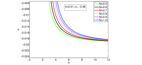
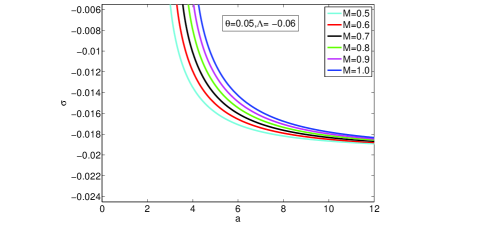
Figure 1: Surface Energy density $\sigma$ has been plotted against $a$ for different values of mass $M$ when noncommutative parameter $\theta=0.01$ (left) and for $\theta=0.05$ (right).

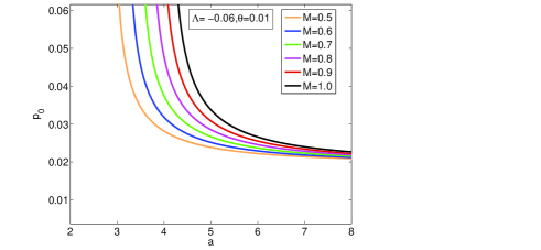
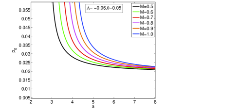
Figure 2: Surface Pressure $p$ has been plotted against $a$ for different values of mass $M$ when noncommutative parameter $\theta=0.01$ (left) and for $\theta=0.05$ (right).

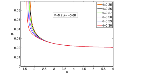
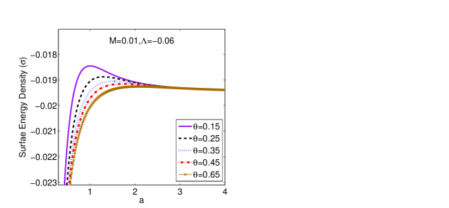
Figure 3: Surface Pressure $p$ has been plotted against $a$ for different values of noncommutative parameter $\theta$ when mass (M) is fixed (left) and surface energy density $\sigma$ has been plotted against $a$ for different values of noncommutative parameter $\theta$ when mass (M) is fixed (right).

III The Gravitational Field

In this section we analyze the attractive or repulsive nature of the wormhole. For this analysis we calculate the observer’s three acceleration $a^{\mu}=u^{\mu}_{~{};\nu}u^{\nu}$, where $u^{\nu}$ is given by

$$u^{\nu}=\frac{dx^{\nu}}{d\tau}=\left(\frac{1}{\sqrt{f(r)}},0,0\right).$$ (15)

The only non-zero component is given by

$$a^{r}=\Gamma_{tt}^{r}=\frac{1}{2}f^{\prime}(r)=-\frac{Mr}{2\theta}e^{-\frac{r^{2}}{4\theta}}-\Lambda r,$$ (16)

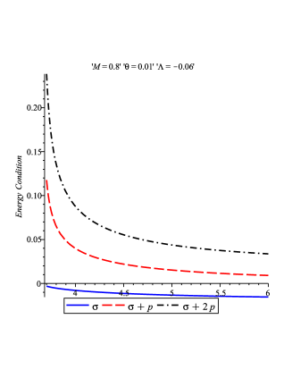
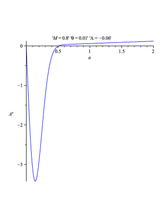
Figure 4: Energy condition is plotted against ‘a’ (left) and $a^{r}$ is plotted against ‘a’(right).

A test particle when radially moving and initially at rest, obeys the equation of motion

$$\frac{d^{2}r}{d\tau^{2}}=-A^{r}=\frac{Mr}{2\theta}e^{-\frac{r^{2}}{4\theta}}+\Lambda r.$$ (17)

If $A^{r}=0$, we get the geodesic equation and solving the eq. (16), for r we obtain

$$r=\pm\sqrt{-4\theta\ln\left(-\frac{2\theta\Lambda}{M}\right)}.$$ (18)

Here we consider only positive sign to find the value of ‘r’ since it was previously assumed $a>r_{h}$.
Now, the wormhole will be attractive in nature if $A^{r}>0$ i.e., ‘r’ satisfying the following condition

$$\sqrt{-4\theta\ln\left(-\frac{2\theta\Lambda}{M}\right)}<r<\infty,$$ (19)

and similarly, the wormhole will be repulsive in nature if $A^{r}<0$, which is given by

$$0<r<\sqrt{-4\theta\ln\left(-\frac{2\theta\Lambda}{M}\right)}.$$ (20)

The Eqs. (18)-(20) will be valid only if $\left|-\frac{2\theta\Lambda}{M}\right|<1$. Fig. 4 (right) shows that the curve cuts the ‘a-axis’ at the point $a=\pm 0.5$ for a fixed value of M = 0.8, $\theta$ = 0.01, and $\Lambda$ = -0.06. Hence, the wormhole will be attractive for $0.5<a<\infty$ and repulsive for $0<a<0.5$.

IV Total amount of Exotic Matter

To construct thin-shell wormholes, we determine the total amount of exotic matter. Though, using noncommutative BTZ black hole in the thin-shell wormhole construction is that, it is not asymptotically flat and therefore the wormholes are not asymptotically flat. Recently Mazharimousavi, Halilsoy and Amirabi Mazharimousavi shown that a non-asymptotically flat black hole solution provides stable thin-shell wormholes which are entirely supported by exotic matter and quantified by the integral KY ; ES ; MC ; FK

$$\Omega=\int[\rho+p_{r}]\sqrt{-g}d^{2}x,$$ (21)

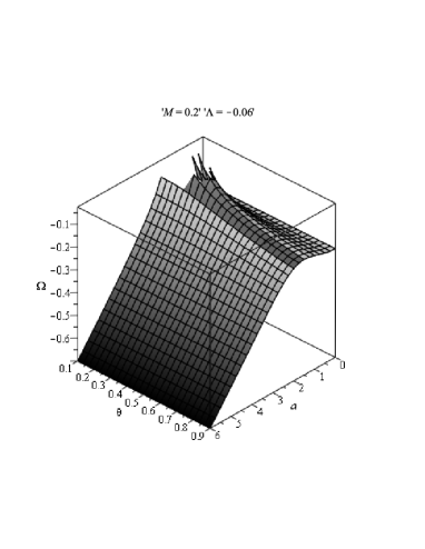
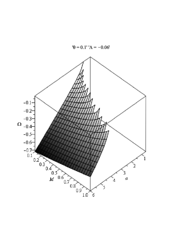
Figure 5: The variation of total amount of exotic matter $\Omega$ has been plotted against $a$ for different values of $\theta$ when mass $M$ is fixed (left) and for different values of mass (M) when noncommutative parameter $\theta$ is fixed (right).

where $g$ represents the determinant of the metric tensor. Now, by introducing the radial coordinate $R=r-a$, we have

$$\Omega=\int_{0}^{2\pi}\int_{-\infty}^{\infty}[\rho+p_{r}]\sqrt{-g}~{}dRd\phi.$$ (22)

Since the shell is infinitely thin, it does not exert any radial pressure, i.e., $p_{r}=0$ and using $\rho=\delta(R)\sigma(a)$ for the above integral we have

$$\Omega=\int_{0}^{2\pi}[\rho\sqrt{g}]|_{r=a}d\phi=2\pi a\sigma(a)=-\frac{1}{2}\sqrt{M\left(2e^{-\frac{a^{2}}{4\theta}}-1\right)-\Lambda r^{2}}.$$ (23)

From Eq. (23), one can see that the total amount of exotic matter depends on the mass of the black hole and the noncommutative parameter $\theta$. With the help of graphical representation (see Fig. (5)) we are trying to describe the variation of the total amount of exotic matter in the shell with respect to the mass of the black hole M and the noncommutative parameter $\theta$. It is clear from Fig. (5), that we can reduce the total amount of exotic matter for the shell by increasing the mass M, of the black hole if we fixed the noncommutative parameter $\theta$ or by choosing very small $\theta$, when the mass M is fixed.

So the mass of the black hole M and the noncommutative parameter $\theta$ plays a crucial role to reduce the total amount of exotic matter for the proposed thin-shell wormhole. Furthermore it can be noted that $\Omega\rightarrow 0$ if $a\rightarrow r_{h}$ i.e., if $a$ is very close to the event horizon of the noncommutative BTZ black hole then the required total amount of exotic matter will be infinitesimal small and if $a>>r_{h}$ then $\Omega\rightarrow-\infty$.

V An Equation of State

Taking the form of the equation of state (EoS) to be $p=\omega\sigma$, we obtain from Eqs. $(13)$ and $(14)$

$$\omega=\frac{p}{\sigma}=\frac{a^{2}\left(\frac{M}{2\theta}e^{-\frac{a^{2}}{4\theta}}+\Lambda\right)}{M\left(2e^{-\frac{a^{2}}{4\theta}}-1\right)-\Lambda a^{2}}.$$ (24)

From Eq. $(24)$, we observe that if the location of the wormhole throat is very large i.e., if $a\rightarrow+\infty$ then $\omega\rightarrow-1$ and if $g(a)=0$ at some $a=a_{0}$ where $g(a)=\frac{M}{2\theta}e^{-\frac{a^{2}}{4\theta}}+\Lambda$, then $p\rightarrow 0$, but in that case $a_{0}<r_{h}$ (see Fig.(6)). So dust shell is never found.

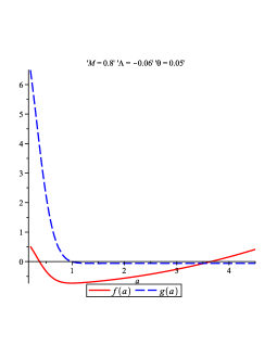
Figure 6: The curve $g(a)$ cuts the ’a’ axis at a point $a_{0}<r_{h}$

VI stability Analysis

In this section we turn to the question of stability of the wormhole using two different approaches: (i) assuming a specific equation of state on the thin shell and (ii) analyzing the stability to linearized radial perturbations.

VI.1 Dark energy equation of State

As the negative surface energy density supports the presence of exotic matter at the throat, we want to study specific cases by giving an equation of state rather than the analysis for a general equation of state of the form p= p($\sigma$). For the dynamical characterization of the shell, we consider the dark energy as exotic matter on the shell which is governed by an equation of state of the form

$$p=\omega\sigma~{}~{}~{}~{}\text{with}~{}~{}~{}\omega<0,$$ (25)

which is a possible candidate for the accelerated expansion of the Universe and consequently violates the null energy condition. Such a dark energy fluid can be divided into three cases: a normal dark energy fluid when -1 $<\omega<$ 0, a cosmological constant fluid when $\omega=-1$, and a phantom energy fluid when $\omega<-1$ . Now, using the Eqs. (25) into (12), we obtain

$$\sigma=\sigma_{0}\left(\frac{a_{0}}{a}\right)^{1+\omega},$$ (26)

where $a=a_{0}$ is the static solution and $\sigma_{0}=\sigma(a_{0})$. Rearranging Eq. $(9)$, one can obtain

$$\dot{a}^{2}+V(a)=0,$$ (27)

where the potential V(a) is defined by

$$V(a)=f(a)-16\pi^{2}a^{2}\sigma^{2}.$$ (28)

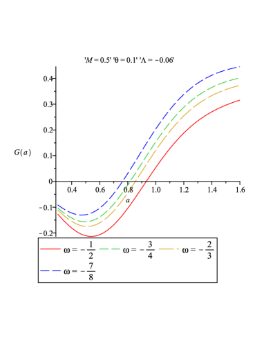
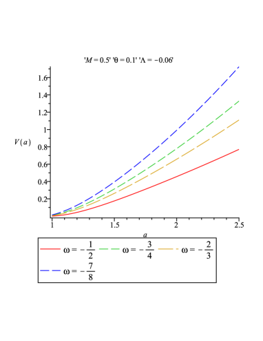
Figure 7: The throat of the thin-shell-wormhole occurs where ‘G(a)’ cuts the ‘a’ axis (Left) and wormholes collapse for the value of $-1<\omega<-\frac{1}{3}$.

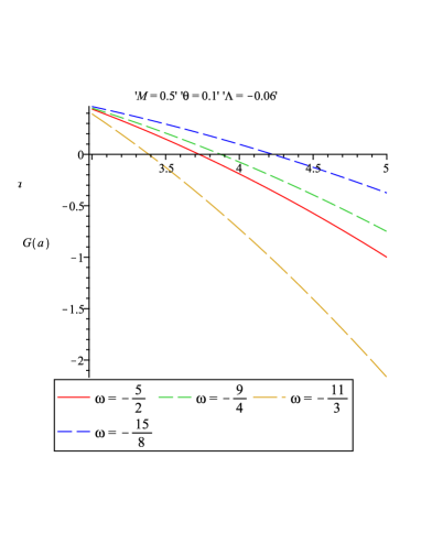
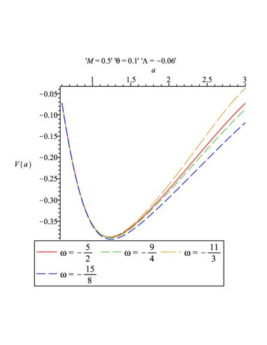
Figure 8: The throat of the thin-shell-wormhole occurs where ‘G(a)’ cuts the ‘a’ axis (Left) and wormholes are stable for the value of $\omega<-1$.

Now employing the Eq. $(26)$ into $(28)$ and substitute the value of $\sigma(a)$, we get

$$V(a)=M\left[2e^{-\frac{a^{2}}{4\theta}}-1\right]-\Lambda a^{2}-\left(\frac{a_{0}}{a}\right)^{2\omega}\left[M\left(2e^{-\frac{a_{0}^{2}}{4\theta}}-1\right)-\Lambda a_{0}^{2}\right].$$ (29)

For the linearized stability criteria, we use Taylor expansion to V (a) (upto second order) around the static solution at $a=a_{0}$, we obtain

$$V(a)=V(a_{0})+(a-a_{0})V^{\prime}(a_{0})+\frac{(a-a_{0})^{2}}{2}V^{\prime\prime}(a_{0})+O[(a-a_{0})^{3}],$$ (30)

where prime denotes derivative with respect to ‘a’. The wormhole is stable if and only if $V(a_{0})$ has local minimum at $a_{0}$ and $V^{\prime\prime}(a_{0})>0$. From Eq. (29) the first derivative of V (a) is

$$V^{\prime}(a)=-\frac{Ma}{\theta}e^{-\frac{a^{2}}{4\theta}}-2a\Lambda+2\omega a_{0}^{2\omega}\left[M\left(2e^{-\frac{a_{0}^{2}}{4\theta}}-1\right)-\Lambda a_{0}^{2}\right]a^{-2\omega-1}.$$ (31)

The second derivative of the potential is

$$V^{\prime\prime}(a_{0})=-\frac{M}{\theta}\left[1-\frac{a_{0}^{2}}{2\theta}\right]e^{-\frac{a_{0}^{2}}{4\theta}}-2\Lambda-\frac{2\omega(2\omega+1)}{a_{0}^{2}}\left[M\left(2e^{-\frac{a_{0}^{2}}{4\theta}}-1\right)-\Lambda a_{0}^{2}\right].$$ (32)

Now the configuration will be stable if and only if $V^{\prime\prime}(a_{0})>0$ for the choice of parameters M, $\theta$ and $\omega$. We are trying to describe the stability of the configuration with help of graphical representation due to complexity of the expression. In Figs. 7-8, we plot the graphs to find the possible range of $a_{0}$ where V $(a_{0})$ possess a local minimum. Using the Eq. (25), we obtain the throat radius of the shell at some a = $a_{0}$ when G(a) cuts the the a-axis which represents the radius of the throat of shell and using the value of $a_{0}$ we find that V$(a_{0})$ posses a local minima when $\omega~{}<-1$ for different values of $\omega$, respectively. Thus, we can obtain stable thin-shell wormholes supported by exotic matter filled with phantom energy EOS.

VI.2 Linearized Stability

We shall study the stability of the configuration under small perturbations around the static solution i.e., $a=a_{0}$, preserving the symmetry. Applying the Taylor series expansion for the potential $V(a)$ upto second order around the stable solution at $a=a_{0}$, which provides

$$V(a)=V(a_{0})+(a-a_{0})V^{\prime}(a_{0})+\frac{(a-a_{0})^{2}}{2}V^{\prime\prime}(a_{0})+O[(a-a_{0})^{3}],$$ (33)

where the prime denotes derivative with respect to $d/da$ and $a_{0}$ is the radius of the static solution. Since we are linearizing around $a=a_{0}$, the stability of static solutions requires $V(a_{0})=0$, $V^{\prime}(a_{0})=0$. Now, the wormhole is stable if and only if $V^{\prime\prime}(a_{0})>0$. To know whether the equilibrium solution is stable or not, we shall follow the procedure adapted by Poisson and Visser Poisson . The physical interpretation of $\beta^{2}$ is a matter of some subtlety which we shall subsequently discuss. First of all we shall restrict ourselves only to the case when $\beta^{2}>0$. The parameter $\beta^{2}$, when lies in the range of $0<\beta^{2}\leq 1$, it can be interpreted as the square of the velocity of sound on the shell and the interpretation is not valid when $\beta^{2}>1$, because it would mean a speed greater than the velocity of light, implying the violation of causality. Now defining the parameter $\beta^{2}$ by

$$\beta^{2}=\frac{\partial p}{\partial\sigma}\Bigl{\lvert}_{\sigma}.$$ (34)

Since $\sigma^{\prime}={\dot{\sigma}/\dot{a}}$, using the Eq. (12), we have $\dot{\sigma}=-\frac{\dot{a}}{a}(\sigma+p)$. The second derivative of the potential is

$$V^{\prime\prime}(a)=-\frac{M}{\theta}e^{-\frac{a^{2}}{4\theta}}\left(1-\frac{a^{2}}{2\theta}\right)-2\Lambda-32\pi^{2}p^{2}-32\pi^{2}\beta^{2}\sigma(p+\sigma).$$ (35)

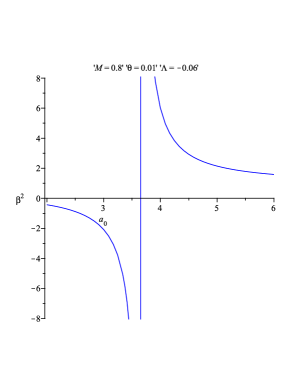
Figure 9: Stability regions for thin-shell wormholes corresponding to $M=0.8$, $\theta=0.01$ and $\Lambda=-0.06$.

Since we are linearizing around $a=a_{0}$, we require that $V(a_{0})=0$ and $V^{\prime}(a_{0})=0$.

Now the configuration will be stable if $V^{\prime\prime}(a_{0})>0$, which gives

$$\beta^{2}<\frac{-\frac{M}{\theta}e^{-\frac{a^{2}}{4\theta}}(1-\frac{a^{2}}{2\theta})-2\Lambda-32\pi^{2}p^{2}}{32\pi^{2}\sigma(\sigma+p)}~{}~{}~{}~{}~{}~{}~{}if~{}(\sigma+p)<0,$$ (36)

and

$$\beta^{2}>\frac{-\frac{M}{\theta}e^{-\frac{a^{2}}{4\theta}}(1-\frac{a^{2}}{2\theta})-2\Lambda-32\pi^{2}p^{2}}{32\pi^{2}\sigma(\sigma+p)}~{}~{}~{}~{}~{}~{}~{}~{}~{}if~{}(\sigma+p)>0,$$ (37)

Now using the values of $\sigma$ and $p$ from Eqs. (13) and (14), and solve for $\beta^{2}$ by letting $V^{\prime\prime}(a_{0})=0$, we have

$$\beta^{2}=\frac{1}{\frac{2M}{a_{0}^{2}}\left[\frac{a_{0}^{2}}{2\theta}e^{-\frac{a_{0}^{2}}{4\theta}}+2e^{-\frac{a_{0}^{2}}{4\theta}-1}\right]}\left[-\frac{M}{\theta}e^{-\frac{a_{0}^{2}}{4\theta}}\left(1-\frac{a_{0}^{2}}{2\theta}\right)-2\Lambda-2\frac{\left(-\Lambda a_{0}-\frac{Ma_{0}}{2\theta}e^{-\frac{a_{0}^{2}}{4\theta}}\right)^{2}}{M\left(2e^{-\frac{a_{0}^{2}}{4\theta}}-1\right)-\Lambda a_{0}^{2}}\right].$$ (38)

Since $\beta$ represents the velocity of the sound so it is expected that $0<\beta^{2}\leq 1$ . The profile of $\beta^{2}$ is shown in Fig. 9, for fixed values of the parameters $M=0.8$, $\theta=0.01$ and $\Lambda=-0.06$. Since Fig. (4) shows that $\sigma+p>0$, so for our model the stability region is given by equation (37) i.e., our model is stable above the curve on the right side of the asymptotes and below the curve of the left side of the asymptotes of Fig. (9). In this case we have $\beta^{2}>1$. As we are dealing with exotic matter, we relaxed the range of $\beta^{2}$ in our stability analysis for the thin-shell wormholes.

VI.3 SUMMARY AND DISCUSSION

In this work, we have taken a noncommutative BTZ black hole solution of the (2+1)-dimensional gravity and followed the cut and paste method for removing the singular part of this manifold in order to construct thin-shell wormholes under the assumption that the equations of state on the shell which defines the throat have the same form as in the static case when it is perturbed preserving the symmetry. Though, a disadvantage with using noncommutative BTZ black holes in the thin-shell wormholes construction is that it is not asymptotically flat and therefore the wormholes are not asymptotically flat. Therefore, there is some matter at infinity. The construction allows a graphical description of both $\sigma$ and p as functions of the radius a of the thin shell, using various values of the mass M and the noncommutative parameter $\theta$. Also we get from Fig. 4 (left) that $\sigma$+p $>0$ and $\sigma$+2p $>0$ are positive which shows matter contained by the shell violates the WEC but satisfy the NEC and SEC. Using the same parameters we determine whether the wormhole is attractive or repulsive. Finally, the total amount of exotic matter required is determined both analytically and graphically with respect to mass and noncommutative parameter.

We draw our main attention on the stability of the shell: It is observed that the matter distribution of the shell is phantom energy type $p=\omega\sigma$ with $\omega<0$, and the stability of the static configurations under radial perturbations was analyzed using the standard potential method and shown that stable wormholes found for $\omega<-1$ in Fig. (8). Next, we have addressed the issue of stability of static configurations under radial perturbations with a linearized equation of state around the static solution i.e., at a=$a_{0}$. The stability analysis concentrated on the parameter $\beta^{2}$, ranges of the parameters for which the stability regions include is $0<\beta^{2}<1$, interpreted as the speed of sound on the shell. We found that stable solutions exist if we relax the range of the parameter $\beta^{2}$, which is not clear to us for exotic matter.

VI.4 Acknowledgments

The authors are thankful to the anonymous referees for their valuable comments to improve the manuscript. AB wishes to thank the authorities of the Inter-University Centre for Astronomy and Astrophysics, Pune, India, for providing Visiting fellowship under which a part of this work was carried out.