Climbing down Gaussian peaks

Abstract

How likely is the high level of a continuous Gaussian random field on an Euclidean space to have a “hole” of a certain dimension and depth? Questions of this type are difficult, but in this paper we make progress on questions shedding new light in existence of holes. How likely is the field to be above a high level on one compact set (e.g. a sphere) and to be below a fraction of that level on some other compact set, e.g. at the center of the corresponding ball? How likely is the field to be below that fraction of the level anywhere inside the ball? We work on the level of large deviations.

Climbing down Gaussian peaks

and t1Research supported in part by US-Israel Binational Science Foundation, 2008262 t2Research supported in part by ARO grant W911NF-12-10385 and NSF grant DMS-1005903 at Cornell University. t4Research supported in part by URSAT, ERC Advanced Grant 320422.

Adler and Samorodnitsky

[class=AMS] [Primary ]60G15, 60F10; [Secondary ]60G60, 60G70, 60G17. Gaussian process, excursion set, large deviations, exceedence probabilities, topology.

1 Introduction

Let $T$ be a compact subset of ${\mathbb{R}}^{d}$. For a real-valued sample continuous random field ${\bf X}=(X({\bf t}),\,{\bf t}\in T)$ and a level $u$, the excursion set of ${\bf X}$ above the level $u$ is the random set

$$A_{u}=\bigl{\{}{\bf t}\in T:\,X({\bf t})>u\bigr{\}}\,.$$ (1.1)

Assuming that the entire index set $T$ has no interesting topological features (i.e., $T$ is homotopic to a ball), what is the structure of the excursion set? This is a generally difficult and important question, and it constitutes an active research area. See Adler and Taylor (2007) and Azaïs and Wschebor (2009) for in-depth discussions. In this paper we consider the case when the random field ${\bf X}$ is Gaussian. Even in this case the problem is still difficult.

In a previous paper Adler et al. (2014) we studied a certain connectedness property of the excursion set $A_{u}$ for high level $u$. Specifically, given two distinct points in ${\mathbb{R}}^{d}$, say, ${\bf a}$ and ${\bf b}$, we studied the asymptotic behaviour, as $u\to\infty$, of the conditional probability that, given $X({\bf a})>u$ and $X({\bf b})>u$, there exists a path $\xi$ between ${\bf a}$ and ${\bf b}$ such that $X({\bf t})>u$ for every ${\bf t}\in\xi$.

In contrast, in this paper our goal is to study the probability that the excursion set $A_{u}$ has holes of a certain size over which the random field drops a fraction of the level $u$. We start with some examples of the types of probabilities we will look at. We will use the following notation. For an Euclidean ball $B$ will denote by $c_{B}$ its center and by $S_{B}=\partial(B)$ the sphere forming its boundary. Consider the following probabilities. For $0<r\leq 1$ denote

$$\Psi_{\text{s}p}(u;r)=P\left(\text{there exists a ball $B$ entirely in $T$ }\right.$$ (1.2)

$$\left.\text{ such that $X({\bf t})>u$ for all ${\bf t}\in S_{B}$ but $X({\bf s})<ru$ for some ${\bf s}\in B$}\right)$$

and

$$\Psi_{\text{s}p;c}(u;r)=P\left(\text{there exists a ball $B$ entirely in $T$ }\right.$$ (1.3)

$$\left.\text{ such that $X({\bf t})>u$ for all ${\bf t}\in S_{B}$ but $X(c_{B})<ru$}\right)\,.$$

Simple arguments involving continuity show that the relevant sets in both (1.2) and (1.3) are measurable. Therefore, the probabilities $\Psi_{\text{s}p}(u;\tau)$ and $\Psi_{\text{s}p;c}(u;\tau)$ are well defined. These are the probabilities of events that, for some ball, the boundary of the ball belongs to the excursion set $A_{u}$, but the excursion set has a hole somewhere inside the ball in one case, containing the center of the ball in another case, in which the value of the field drops below $\tau u$.

We study the logarithmic behaviour of probabilities of this type by using the large deviation approach. We start with a setup somewhat more general than that described above. Specifically, let ${\mathcal{C}}$ be a collection of ordered pairs $(K_{1},K_{2})$ of nonempty compact subsets of $T$. We denote, for $0<r\leq 1$,

$$\Psi_{{\mathcal{C}}}(u;r)=P\left(\text{ there is $(K_{1},K_{2})\in{\mathcal{C}}$ such that }\right.$$ (1.4)

$$\left.\text{ $X({\bf t})>u$ for each ${\bf t}\in K_{1}$ and $X({\bf t})<ru$ for each ${\bf t}\in K_{2}$.}\right)$$

We note that the probabilities $\Psi_{\text{s}p}(u;r)$ and $\Psi_{\text{s}p;c}(u;r)$ are special cases of the probability $\Psi_{{\mathcal{C}}}(u;r)$ with the collections ${\mathcal{C}}$ being, respectively,

$${\mathcal{C}}=\Bigl{\{}\bigl{(}S_{B},{\bf s}\bigr{)},\ \text{ $B$ a ball entirely in $T$ and ${\bf s}\in B$}\Bigr{\}}$$

and

$${\mathcal{C}}=\Bigl{\{}\bigl{(}S_{B},c_{B}\bigr{)},\ \text{ $B$ a ball entirely in $T$ }\Bigr{\}}\,.$$

In Section 2 we first introduce the necessary technical background, and then prove a large deviation result in the space of continuous functions for the probability $\Psi_{{\mathcal{C}}}(u;r)$. This result establishes a connection of the asymptotic behaviour of the probability $\Psi_{{\mathcal{C}}}(u;r)$ to a certain optimization problem. The dual formulation of this problem involves optimization over a family of probability measures, and in Section 3 we describe important properties of the measures that are optimal for the dual problem. The general theory developed in these two sections leads to particularly transparent and intuitive results when applied to isotropic Gaussian fields. This is explored in Section 4.

2 A large deviations result

Consider a real-valued centered continuous Gaussian random field indexed by a compact subset $T\subset{\mathbb{R}}^{d}$, ${\bf X}=(X({\bf t}),\,{\bf t}\in T)$. We denote the covariance function of ${\bf X}$ by $R_{\bf X}({\bf s},{\bf t})=\text{cov}(X({\bf s}),X({\bf t}))$. We view ${\bf X}$ as a Gaussian random element in the space $C(T)$ of continuous functions on $T$, equipped with the supremum norm, whose law is a Gaussian probability measure $\mu_{\bf X}$ on $C(T)$. See e.g. van der Vaart and van Zanten (2008) about this change of the viewpoint, and for more information on the subsequent discussion.

The reproducing kernel Hilbert space (henceforth RKHS) ${\mathcal{H}}$ of the Gaussian measure $\mu_{\bf X}$ (or of the random field ${\bf X}$) is a subspace of $C(T)$ obtained as follows. We identify ${\mathcal{H}}$ with the closure $\mathcal{L}$ in the mean square norm of the space of finite linear combinations $\sum_{j=1}^{k}a_{j}X({\bf t}_{j})$ of the values of the process, $a_{j}\in{\mathbb{R}},\,{\bf t}_{j}\in T$ for $j=1,\ldots,k$, $k=1,2,\ldots$ via the injection ${\mathcal{L}}\to C(T)$ given by

$$H\to w_{H}=\Bigl{(}E\bigl{(}X({\bf t})H\bigr{)},\ {\bf t}\in T\Bigr{)}\,.$$ (2.5)

We denote by $(\cdot,\cdot)_{\mathcal{H}}$ and $\|\cdot\|_{\mathcal{H}}$ the inner product and the norm in the RKHS ${\mathcal{H}}$. By definition,

$$\|w_{H}\|^{2}_{\mathcal{H}}\ =\ E(H^{2})\,.$$ (2.6)

The “reproducing property” of the space ${\mathcal{H}}$ is a consequence of the following observations. For every ${\bf t}\in{\mathbb{R}}^{d}$, the fixed ${\bf t}$ covariance function $R_{{\bf t}}=R(\cdot,{\bf t})$ is in ${\mathcal{H}}$. Therefore, for every $w_{H}\in{\mathcal{H}}$, and ${\bf t}\in{\mathbb{R}}^{d}$, $w_{H}({\bf t})=(w_{H},R_{\bf t})_{\mathcal{H}}$. In particular, the coordinate projections are continuous operations on the RKHS.

The quadruple $(C(T),{\mathcal{H}},w,\mu_{\bf X})$ is a Wiener quadruple in the sense of Section 3.4 in Deuschel and Stroock (1989). This allows one to use the machinery of large deviations for Gaussian measures described there.

The following result is a straightforward application of the general large deviations machinery.

Theorem 2.1.

Let ${\bf X}=(X({\bf t}),\,{\bf t}\in T)$ be a continuous Gaussian random field on a compact set $T\subset{\mathbb{R}}^{d}$. Let ${\mathcal{C}}$ be a collection of ordered pairs $(K_{1},K_{2})$ of nonempty compact subsets of ${\mathbb{R}}^{d}$, compact in the product Hausdorff distance. Then for $0<r\leq 1$,

$$-\frac{1}{2}\lim_{\tau\uparrow r}D_{{\mathcal{C}}}(\tau)\leq\liminf_{u\to\infty}\frac{1}{u^{2}}\log\Psi_{{\mathcal{C}}}(u;r)$$ (2.7)

$$\leq\limsup_{u\to\infty}\frac{1}{u^{2}}\log\Psi_{{\mathcal{C}}}(u;r)\leq-\frac{1}{2}D_{{\mathcal{C}}}(r)\,,$$

where for $r>0$,

$$D_{{\mathcal{C}}}(r) \stackrel{{\scriptstyle\Delta}}{{=}} \inf\left\{EH^{2}:\,H\in{\mathcal{L}},\ \text{and, for some $(K_{1},K_{2})\in{\mathcal{C}}$, }\right.$$ (2.8)

$$\left.\text{ $E\bigl{(}X({\bf t})H\bigr{)}\geq 1$ for each ${\bf t}\in K_{1}$ and $E\bigl{(}X({\bf t})H\bigr{)}\leq r$ for each ${\bf t}\in K_{2}$}\right\}.$$

Proof.

As is usual in large deviations arguments, we write, for $u>0$,

$$\Psi_{{\mathcal{C}}}(u;r)=P\bigl{(}u^{-1}{\bf X}\in A\bigr{)}\,,$$

where $A$ is the open subset of $C(T)$ given by

$$A\stackrel{{\scriptstyle\Delta}}{{=}}\Bigl{\{}{\bf\omega}\in C(T):\ \text{ there is $(K_{1},K_{2})\in{\mathcal{C}}$ such that }$$

$$\text{ $\omega({\bf t})>1$ for each ${\bf t}\in K_{1}$ and $\omega({\bf t})<r$ for each ${\bf t}\in K_{2}$}\Bigr{\}}.$$

We use Theorem 3.4.5 in Deuschel and Stroock (1989). We have

$$-\inf_{{\bf\omega}\in A}I({\bf\omega})\leq\liminf_{u\to\infty}\frac{1}{u^{2}}\log\Psi_{{\mathcal{C}}}(u;\tau)\leq\limsup_{u\to\infty}\frac{1}{u^{2}}\log\Psi_{{\mathcal{C}}}(u;\tau)\leq-\inf_{{\bf\omega}\in\bar{A}}I({\bf\omega})\,.$$ (2.9)

By Theorem 3.4.12 of Deuschel and Stroock (1989) the rate function $I$ can be written as

$$I({\bf\omega})=\left\{\begin{array}[]{ll}\frac{1}{2}\|{\bf\omega}\|_{\mathcal{H}}^{2}&\text{if ${\bf\omega}\in{\mathcal{H}}$},\\ \infty&\text{if ${\bf\omega}\notin{\mathcal{H}}$,}\end{array}\right.$$ (2.10)

for ${\bf\omega}\in C(T)$. Since ${\mathcal{C}}$ is compact in the product Hausdorff distance,

$$\bar{A}\subseteq\Bigl{\{}{\bf\omega}\in C(T):\ \text{ there is $(K_{1},K_{2})\in{\mathcal{C}}$ such that }$$

$$\text{ $\omega({\bf t})\geq 1$ for each ${\bf t}\in K_{1}$ and $\omega({\bf t})\leq r$ for each ${\bf t}\in K_{2}$}\Bigr{\}},$$

and so (2.9) already contains the upper limit statement in (2.7). Further, for any $0<\varepsilon<1$,

$$\inf_{{\bf\omega}\in A}I({\bf\omega})\leq\inf\left\{EH^{2}:\,H\in{\mathcal{L}},\ \text{and, for some $(K_{1},K_{2})\in{\mathcal{C}}$, }\right.$$

$$\left.\text{ $\omega_{H}({\bf t})\geq 1+\varepsilon$ for each ${\bf t}\in K_{1}$ and $\omega_{H}({\bf t})\leq(1-\varepsilon)r$ for each ${\bf t}\in K_{2}$}\right\}$$

$$=(1+\varepsilon)^{2}D_{{\mathcal{C}}}\left(\frac{1-\varepsilon}{1+\varepsilon}r\right)\,.$$

Letting $\varepsilon\downarrow 0$ establishes the lower limit statement in (2.7). ∎

The lower bound in (2.7) can be strictly smaller than the upper bound, as the following example shows. We will see in the sequel that in certain cases of interest the two bounds do coincide.

Example 2.2.

Let $T=\{0,1,2\}$. Starting with independent standard normal random variables $Y_{1},Y_{2}$ we define, for $0<r_{0}<1$ and $\sigma>r_{0}$,

$$X(0)=Y_{1},\ X(1)=r_{0}Y_{1},\ X(2)=\sigma Y_{1}+Y_{2}\,.$$

Note that in this case ${\mathcal{L}}=\{a_{1}Y_{1}+a_{2}Y_{2},\ a_{1}\in{\mathbb{R}},\,a_{2}\in{\mathbb{R}}\}$.

Let ${\mathcal{C}}=\bigl{\{}\bigl{(}\{0\},\{1\}\bigr{)},\,\bigl{(}\{0\},\{2\}\bigr{)}\bigr{\}}$. It is elementary to check that

$$D_{{\mathcal{C}}}(r)=\left\{\begin{array}[]{ll}1+(\sigma-r)^{2}&\text{for $0<r<r_{0}$,}\\ 1&\text{for $r\geq r_{0}$,}\end{array}\right.$$

and that this function is not left continuous at $r=r_{0}$.

For a fixed pair $(K_{1},K_{2})\in{\mathcal{C}}$ denote

$$D_{K_{1},K_{2}}(r)=\inf\left\{EH^{2}:\,H\in{\mathcal{L}}\ \text{such that}\right.$$ (2.11)

$$\left.\text{ $E\bigl{(}X({\bf t})H\bigr{)}\geq 1$ for each ${\bf t}\in K_{1}$ and $E\bigl{(}X({\bf t})H\bigr{)}\leq r$ for each ${\bf t}\in K_{2}$}\right\}.$$

Clearly,

$$D_{{\mathcal{C}}}(r)=\min_{(K_{1},K_{2})\in{\mathcal{C}}}D_{K_{1},K_{2}}(r)\,,$$ (2.12)

with the minimum actually achieved. Furthermore, an application of Theorem 2.1 to the case of ${\mathcal{C}}$ consisting of a single ordered pair of sets immediately shows that

$$-\frac{1}{2}\lim_{\tau\uparrow r}D_{K_{1},K_{2}}(\tau) \leq\liminf_{u\to\infty}\frac{1}{u^{2}}\log\Psi_{K_{1},K_{2}}(u;r)$$ (2.13)

$$\leq\limsup_{u\to\infty}\frac{1}{u^{2}}\log\Psi_{K_{1},K_{2}}(u;r)\leq-\frac{1}{2}D_{K_{1},K_{2}}(r)\,,$$

where

$$\Psi_{K_{1},K_{2}}(u;r)=P\left(\text{ $X({\bf t})>u$ for all ${\bf t}\in K_{1}$ and $X({\bf t})<ru$ for all ${\bf t}\in K_{2}$.}\right)$$

The next result describes useful properties of the function $D_{K_{1},K_{2}}$.

Theorem 2.3.

(a) If the feasible set in (2.11) is not empty, then the infimum is achieved, at a unique $H\in{\mathcal{L}}$.

(b)  The following holds true:

$$D_{K_{1},K_{2}}(r)=\left\{\min\left[\min_{\mu_{1}\in M_{1}^{+}(K_{1})}\int_{K_{1}}\int_{K_{1}}R_{\bf X}({\bf t}_{1},{\bf t}_{2})\,\mu_{1}(d{\bf t}_{1})\mu_{1}(d{\bf t}_{2}),\ \right.\right.$$ (2.14)

$$\left.\left.\min_{\mu_{1}\in M_{1}^{+}(K_{1}),\mu_{2}\in M_{1}^{+}(K_{2})\atop\text{\rm subject to \eqref{e:cond.1}}}\frac{A_{K_{1},K_{2}}(\mu_{1},\mu_{2})}{B_{K_{1},K_{2}}(\mu_{1},\mu_{2};r)}\right]\right\}^{-1}$$

with

$$A_{K_{1},K_{2}}(\mu_{1},\mu_{2})=$$

$$\int_{K_{1}}\int_{K_{1}}R_{\bf X}({\bf t}_{1},{\bf t}_{2})\,\mu_{1}(d{\bf t}_{1})\mu_{1}(d{\bf t}_{2})\int_{K_{2}}\int_{K_{2}}R_{\bf X}({\bf t}_{1},{\bf t}_{2})\,\mu_{2}(d{\bf t}_{1})\mu_{2}(d{\bf t}_{2})$$

$$-\left(\int_{K_{1}}\int_{K_{2}}R_{\bf X}({\bf t}_{1},{\bf t}_{2})\,\mu_{1}(d{\bf t}_{1})\mu_{2}(d{\bf t}_{2})\right)^{2},$$

$$B_{K_{1},K_{2}}(\mu_{1},\mu_{2};r)=$$

$$r^{2}\int_{K_{1}}\int_{K_{1}}R_{\bf X}({\bf t}_{1},{\bf t}_{2})\,\mu_{1}(d{\bf t}_{1})\mu_{1}(d{\bf t}_{2})-2r\int_{K_{1}}\int_{K_{2}}R_{\bf X}({\bf t}_{1},{\bf t}_{2})\,\mu_{1}(d{\bf t}_{1})\mu_{2}(d{\bf t}_{2})$$

$$+\int_{K_{2}}\int_{K_{2}}R_{\bf X}({\bf t}_{1},{\bf t}_{2})\,\mu_{2}(d{\bf t}_{1})\mu_{2}(d{\bf t}_{2}),$$

and the condition in the minimization problem is

$$\int_{K_{1}}\int_{K_{2}}R_{\bf X}({\bf t}_{1},{\bf t}_{2})\,\mu_{1}(d{\bf t}_{1})\mu_{2}(d{\bf t}_{2})\geq r\int_{K_{1}}\int_{K_{1}}R_{\bf X}({\bf t}_{1},{\bf t}_{2})\,\mu_{1}(d{\bf t}_{1})\mu_{1}(d{\bf t}_{2})\,.$$ (2.15)

Proof.

For part (a), let $(H_{n})\subset{\mathcal{L}}$ be a sequence of elements satisfying the constraints in (2.11) such that $EH_{n}^{2}\to D_{K_{1},K_{2}}(r)$ as $n\to\infty$. By the Banach - Alaoglu theorem (see e.g. Theorem 2, p. 424 in Dunford and Schwartz (1988)), the sequence $(H_{n})$ is weakly relatively compact in $\mathcal{L}$, and so there is $H\in{\mathcal{L}}$ and a subsequence $n_{k}\to\infty$ such that $E(H_{n_{k}}Y)\to E(HY)$ as $k\to\infty$ for each $Y\in{\mathcal{L}}$. Further, $EH^{2}\leq\liminf_{k\to\infty}EH_{n_{k}}^{2}=D_{K_{1},K_{2}}(r)$. Therefore, $H$ is an optimal solution to the problem (2.11). The uniqueness of $H$ follows from the convexity of the norm.

For part (b) we will use the Lagrange duality approach of Section 8.6 in Luenberger (1969). Let ${\tt Z}=C(K_{1})\times C(K_{2})$, which we equip with the norm $\|(\varphi_{1},\varphi_{2})\|_{\tt Z}=\max\bigl{(}\|\varphi_{1}\|_{C(K_{1})},\|\varphi_{2}\|_{C(K_{2})}\bigr{)}$. Consider the closed convex cone in $\tt Z$ defined by ${\tt P}=\{(\varphi_{1},\varphi_{2}):\,\varphi_{i}(t)\geq 0$ for all $t\in K_{i},\ i=1,2\}$. Its dual cone, which is a subset of ${\tt Z}^{*}$, can be identified with $M^{+}(K_{1})\times M^{+}(K_{2})$, under the action

$$(\mu_{1},\mu_{2})\bigl{(}(\varphi_{1},\varphi_{2})\bigr{)}=\int_{K_{1}}\varphi_{1}\,d\mu_{1}+\int_{K_{2}}\varphi_{2}\,d\mu_{2}$$

for a finite measure $\mu_{i}$ on $K_{i}$, $i=1,2$. Define a convex mapping $G:\,{\mathcal{L}}\to{\tt Z}$ by

$$G(H)=\Bigl{(}\bigl{(}1-w_{H}({\bf t}),\,{\bf t}\in K_{1}\bigr{)},\ \bigl{(}w_{H}({\bf t})-r,\,{\bf t}\in K_{2}\bigr{)}\Bigr{)}.$$

We can write

$$\bigl{(}D_{K_{1},K_{2}}(r)\bigr{)}^{1/2}=\inf\left\{(EH^{2})^{1/2}\,:H\in{\mathcal{L}},\ G(H)\in-{\tt P}\right\}\,.$$ (2.16)

We start with the assumption that the feasible set in (2.11) and (2.16) is not empty. Let $z>r$, and consider the optimization problems (2.11) and (2.16) for $D_{K_{1},K_{2}}(z)$. The feasible set in these problems has now an interior point, and in this case Theorem 1 (p. 224) in Luenberger (1969) applies. We conclude that

$$\bigl{(}D_{K_{1},K_{2}}(z)\bigr{)}^{1/2}=\max_{\mu_{1}\in M^{+}(K_{1}),\,\mu_{2}\in M^{+}(K_{2})}\inf_{H\in{\mathcal{L}}}\biggl{[}(EH^{2})^{1/2}$$ (2.17)

$$+\int_{K_{1}}\bigl{(}1-w_{H}({\bf t})\bigr{)}\,\mu_{1}(d{\bf t})+\int_{K_{2}}\bigr{(}w_{H}({\bf t})-z\bigr{)}\,\mu_{2}(d{\bf t})\biggr{]}\,,$$

and the “max” notation is legitimate, because the maximum is, in fact, achieved. For $i=1,2$ and $\mu_{i}\in M^{+}(K_{i})$ denote by $\|\mu_{i}\|$ its total mass, and by $\hat{\mu}_{i}\in M_{1}^{+}(K_{i})$ the normalized measure $\hat{\mu}_{i}=\mu_{i}/\|\mu_{i}\|$ (if $\|\mu_{i}\|=0$, we use for $\hat{\mu}_{i}$ an arbitrary fixed probability measure in $M^{+}(K_{i})$). Then

$$\bigl{(}D_{K_{1},K_{2}}(z)\bigr{)}^{1/2}=\max_{\mu_{1}\in M^{+}(K_{1}),\,\mu_{2}\in M^{+}(K_{2})}\biggl{\{}\|\mu_{1}\|-z\|\mu_{2}\|$$

$$+\inf_{H\in{\mathcal{L}}}\left[(EH^{2})^{1/2}-\|\mu_{1}\|\int_{K_{1}}w_{H}({\bf t})\,\hat{\mu}_{1}(d{\bf t})+\|\mu_{2}\|\int_{K_{2}}w_{H}({\bf t})\,\hat{\mu}_{2}(d{\bf t})\right]\biggr{\}}\,.$$

Note that for fixed $\mu_{i}\in M^{+}(K_{i})$, $i=1,2$ we have

$$\inf_{H\in{\mathcal{L}}}\left[(EH^{2})^{1/2}-\|\mu_{1}\|\int_{K_{1}}w_{H}({\bf t})\,\hat{\mu}_{1}(d{\bf t})+\|\mu_{2}\|\int_{K_{2}}w_{H}({\bf t})\,\hat{\mu}_{2}(d{\bf t})\right]$$

$$=\inf_{a\geq 0}a\biggl{\{}1-\sup_{H\in{\mathcal{L}},\,EH^{2}=1}\left[\|\mu_{1}\|\int_{K_{1}}w_{H}({\bf t})\,\hat{\mu}_{1}(d{\bf t})-\|\mu_{2}\|\int_{K_{2}}w_{H}({\bf t})\,\hat{\mu}_{2}(d{\bf t})\right]\biggr{\}}$$

$$=\left\{\begin{array}[]{ll}0&\text{if}\ \sup_{H\in{\mathcal{L}},\,EH^{2}=1}[\ldots]\leq 1\\ -\infty&\text{if}\ \sup_{H\in{\mathcal{L}},\,EH^{2}=1}[\ldots]>1\end{array}\right..$$

Therefore,

$$\begin{array}[]{ll}\bigl{(}D_{K_{1},K_{2}}(z)\bigr{)}^{1/2}=&\max_{\mu_{1}\in M^{+}(K_{1}),\,\mu_{2}\in M^{+}(K_{2})}\ \ \bigl{(}\|\mu_{1}\|-z\|\mu_{2}\|\bigr{)}\\ \\ &\text{subject to}\end{array}$$

$$\sup_{H\in{\mathcal{L}},\,EH^{2}=1}\left[\|\mu_{1}\|\int_{K_{1}}w_{H}({\bf t})\,\hat{\mu}_{1}(d{\bf t})-\|\mu_{2}\|\int_{K_{2}}w_{H}({\bf t})\,\hat{\mu}_{2}(d{\bf t})\right]\leq 1\,.$$

Note that by the reproducing property, for fixed $\mu_{1}\in M^{+}(K_{1}),\,\mu_{2}\in M^{+}(K_{2})$,

$$\sup_{H\in{\mathcal{L}},\,EH^{2}=1}\left[\|\mu_{1}\|\int_{K_{1}}w_{H}({\bf t})\,\hat{\mu}_{1}(d{\bf t})-\|\mu_{2}\|\int_{K_{2}}w_{H}({\bf t})\,\hat{\mu}_{2}(d{\bf t})\right]$$

$$=\sup_{w\in{\mathcal{H}},\,\|w\|_{\mathcal{H}}=1}\left(w,\,\|\mu_{1}\|\int_{K_{1}}R_{\bf t}(\cdot)\,\hat{\mu}_{1}(dt)-\|\mu_{2}\|\int_{K_{2}}R_{\bf t}(\cdot)\,\hat{\mu}_{2}(dt)\right)_{\mathcal{H}}\,.$$

Assuming that the element in the second position in the inner product is nonzero, the supremum is achieved at that element scaled to have a unit norm. Therefore, value of the supremum is

$$\left\|\|\mu_{1}\|\int_{K_{1}}R_{\bf t}(\cdot)\,\hat{\mu}_{1}(dt)-\|\mu_{2}\|\int_{K_{2}}R_{\bf t}(\cdot)\,\hat{\mu}_{2}(dt)\right\|_{\mathcal{H}}\,,$$

which is also trivially the case if the element in the second position in the inner product is the zero element. In any case, using the definition of the norm in ${\mathcal{H}}$, we conclude that

$$\bigl{(}D_{K_{1},K_{2}}(z)\bigr{)}^{1/2}=\max_{m_{1}\geq 0,\,m_{2}\geq 0}\max_{\mu_{1}\in M_{1}^{+}(K_{1}),\,\mu_{2}\in M_{1}^{+}(K_{2})}\ \ \bigl{(}m_{1}-z\,m_{2}\bigr{)}$$

subject to (2.18)

$$m_{1}^{2}\int_{K_{1}}\int_{K_{1}}R_{\bf X}({\bf t}_{1},{\bf t}_{2})\,\mu_{1}(d{\bf t}_{1})\mu_{1}(d{\bf t}_{2})-2m_{1}m_{2}\int_{K_{1}}\int_{K_{2}}R_{\bf X}({\bf t}_{1},{\bf t}_{2})\,\mu_{1}(d{\bf t}_{1})\mu_{2}(d{\bf t}_{2})$$

$$+m_{2}^{2}\int_{K_{2}}\int_{K_{2}}R_{\bf X}({\bf t}_{1},{\bf t}_{2})\,\mu_{2}(d{\bf t}_{1})\mu_{2}(d{\bf t}_{2})\leq 1\,.$$

Next, we show that (2.18) holds for $z=r$ as well. Let $A(z),\ z\geq r$ be the value of the maximum in the right hand side of (2.18). We know that $D_{K_{1},K_{2}}(z)=A(z)^{2}$ for $z>r$. Moreover, it is clear that $A(z)\uparrow A(r)$ as $z\downarrow r$. Therefore, in order to extend (2.18) to $z=r$ it is enough to prove that

$$\lim_{z\downarrow r}D_{K_{1},K_{2}}(z)=D_{K_{1},K_{2}}(r)\,.$$ (2.19)

To this end, choose a sequence $z_{n}\downarrow r$. For $n\geq 1$ there is, by part (a), the optimal solution $H_{n}$ of the problem (2.11) corresponding to $z_{n}$. Appealing to the Banach-Alaoglu theorem, we see that the sequence $(H_{n})$ is weakly relatively compact in $\mathcal{L}$, and so there is $H\in{\mathcal{L}}$ to which it converges weakly along a subsequence. This $H$ is, clearly, feasible in (2.11) for $z=r$. Furthermore, $EH^{2}\leq\lim_{n\to\infty}D_{K_{1},K_{2}}(z_{n})$, implying that $D_{K_{1},K_{2}}(r)\leq\lim_{z\downarrow r}D_{K_{1},K_{2}}(z)$, thus giving us the only nontrivial inequality in (2.19). Therefore, (2.18) holds for $z=r$.

A part of the optimization problem in (2.18) with $z=r$ has the form

$$\max_{m_{1}\geq 0,\,m_{2}\geq 0}\ \ \bigl{(}m_{1}-r\,m_{2}\bigr{)}$$

subject to (2.20)

$$am_{1}^{2}-2bm_{1}m_{2}+cm_{2}^{2}\leq 1$$

for fixed numbers $a\geq 0,\,c\geq 0$ and $b\in{\mathbb{R}}$. In our case,

$$a=\int_{K_{1}}\int_{K_{1}}R_{\bf X}({\bf t}_{1},{\bf t}_{2})\,\mu_{1}(d{\bf t}_{1})\mu_{1}(d{\bf t}_{2}),\ b=\int_{K_{1}}\int_{K_{2}}R_{\bf X}({\bf t}_{1},{\bf t}_{2})\,\mu_{1}(d{\bf t}_{1})\mu_{2}(d{\bf t}_{2})$$

and

$$c=\int_{K_{2}}\int_{K_{2}}R_{\bf X}({\bf t}_{1},{\bf t}_{2})\,\mu_{2}(d{\bf t}_{1})\mu_{2}(d{\bf t}_{2})\,.$$ (2.21)

These specific numbers satisfy the condition

$$b^{2}\leq ac\,,$$ (2.22)

and we will assume that this condition holds in the problem (2.20) we will presently consider.

As a first step, it is clear that replacing the inequality constraint in this problem by the equality constraint

$$a_{2}m_{1}^{2}-2bm_{1}m_{2}+cm_{2}^{2}=1$$

does not change the value of the maximum, so we may work with the equality constraint instead. The resulting problem can be easily solved, e.g. by checking the boundary values $m_{1}=0$ or $m_{2}=0$, and using the Lagrange multipliers if both $m_{1}>0$ and $m_{2}>0$. The resulting value of the maximum in this problem is

$$\begin{array}[]{ll}a^{-1/2}&\text{if}\ \ b\leq ra\\ \left(\frac{c+r^{2}a-2rb}{ac-b^{2}}\right)^{1/2}&\text{if}\ \ b>ra\end{array}.$$ (2.23)

Moreover, it is elementary to check that we always have

$$\left(\frac{c+r^{2}a-2rb}{ac-b^{2}}\right)^{1/2}\geq\frac{1}{a^{1/2}}\,.$$

Substituting (2.23) into (2.18) with $z=r$ and using the values of $a,b,c$ given in (2.22) gives us the representation (2.14).

It remains to consider the case when the feasible set in (2.11) and (2.16) is empty. In this case $D_{K_{1},K_{2}}(r)=\infty$, so we need to prove that the optimal value in the dual problem (2.18) (with $\max$ replaced by $\sup$ in the statement) is infinite as well. For this purpose we use the idea of subconsistency in Section 3 of Anderson (1983). We write the minimization problem (2.11) as a linear program with conic constraints, called $IP$ in that paper, with the following parameters. The space $X={\mathbb{R}}\times{\mathcal{L}}$ is in duality with the itself, $Y=X$. The space $Z=C(K_{1})\times C(K_{2})$ (as above) is in duality with the space $W=M(K_{1})\times M(K_{2})$, the product of the appropriate spaces of finite signed measures. The vector $c\in Y$ has the unity as its ${\mathbb{R}}$ element, and the zero function as its $\mathcal{L}$ element. The function $A:\,X\to Z$ is given by

$$A(\alpha,H)=\Bigl{(}\bigl{(}E(HX({\bf t}),\,{\bf t}\in K_{1}\bigr{)},\,\bigl{(}E(HX({\bf t})),\,{\bf t}\in K_{1}\bigr{)}\Bigr{)},\ \alpha\in{\mathbb{R}},\,H\in{\mathcal{L}}\,.$$

The vector $b\in Z$ is given by a pair of continuous functions, the first one takes the constant value of $1$ over $K_{1}$, while the second one takes the constant value of $r$ over $K_{2}$. The positive cone $Q$ in $Z$ is defined by $Q=C_{+}(K_{1})\times(-C_{+}(K_{2}))$, where $C_{+}(K_{i})$ is the subset of $C(K_{i})$ consisting of nonnegative functions, $i=1,2$. Finally, the positive cone $P$ in $X$ is defined by

$$P=\bigl{\{}(\alpha,H):\,\alpha\geq(EH^{2})^{1/2}\bigr{\}}\,.$$

It is elementary to verify that the dual problem $IP^{*}$ of Anderson (1983) coincides with the maximization problem (2.18).

Note that the dual problem is consistent (has a feasible solution). By Theorem 3 in Section 3 of Anderson (1983) (see a discussion at the end of that section), in order to prove that the optimal value of the dual problem is infinite, we need to rule out the possibility that the original (primal) problem is subconsistent with a finite subvalue. With a view of obtaining a contradiction, assume the subconsistency with a finite subvalue of the primal problem. Then there are sequences $(x_{n})\subset P$ and $(z_{n})\subset Q$ such that $Ax_{n}-z_{n}\to b$ as $n\to\infty$ and the sequence of evaluations $(c,x_{n})$ is bounded from above. With the present parameters, this means that there is a sequence $(H_{n})\subset{\mathcal{L}}$ with the bounded sequence $(EH_{n}^{2})$ of the second moments and two sequences of functions $(\varphi_{i,n})\subset C_{+}(K_{i})$, $i=1,2$, such that, weakly,

$$\bigl{(}E(H_{n}X({\bf t}))-\varphi_{1,n}({\bf t}),\,{\bf t}\in K_{1}\bigr{)}\to\bigl{(}1,\,{\bf t}\in K_{1}\bigr{)}\,,$$

$$\bigl{(}E(H_{n}X({\bf t}))+\varphi_{2,n}({\bf t}),\,{\bf t}\in K_{2}\bigr{)}\to\bigl{(}r,\,{\bf t}\in K_{2}\bigr{)}$$

as $n\to\infty$, with the obvious notation for constant functions. Appealing, once again, to the Banach-Alaoglu theorem, we find that there is $H\in{\mathcal{L}}$ such that, along a subsequence, $H_{n}\to H$ weakly. Since weak convergence implies pointwise convergence, we immediately conclude that $E\bigl{(}X({\bf t})H\bigr{)}\geq 1$ for each ${\bf t}\in K_{1}$ and $E\bigl{(}X({\bf t})H\bigr{)}\leq r$ for each ${\bf t}\in K_{2}$, contradicting the assumption that the feasible set (2.11) is empty. The obtained contradiction completes the proof. ∎

Remark 2.4.

It is an easy calculation to verify that, in the optimization problem (2.20), the optimal solution $(m_{1},m_{2})$ has the following properties. In the case $b\leq ra$ in (2.23) one has $m_{2}=0$, whereas if $b>ra$ in (2.23), then the numbers $m_{1}$ and $m_{2}$ are both positive, and

$$\frac{m_{1}}{m_{2}}=\frac{rb-c}{ra-b}\,.$$

We will find these properties useful in the sequel.

Remark 2.5.

We saw in Example 2.2 that the function $D_{{\mathcal{C}}}$ does not, in general, need to be continuous. However, the arguments used in the proof of Theorem 2.3, together with the compactness in the product Hausdorff distance of the set ${\mathcal{C}}$, show that this function is always right continuous

For a fixed pair $(K_{1},K_{2})\in{\mathcal{C}}$ even the absence of left continuity for the function $D_{K_{1},K_{2}}$ is, in a sense, an exception and not the rule. Left continuity is trivially true at any $r_{0}$ for which the minimization problem (2.11) is infeasible. If that problem is feasible, and it remains feasible for some $r<r_{0}$, then the left continuity at $r_{0}$ still holds. To see this, suppose $r_{n}\uparrow r_{0}$ as $n\to\infty$ is such that for some $0<\varepsilon<\infty$

$$\lim_{n\to\infty}\bigl{(}D_{K_{1},K_{2}}(r_{n})\bigr{)}^{1/2}=\bigl{(}D_{K_{1},K_{2}}(r_{0})\bigr{)}^{1/2}+\varepsilon\,.$$ (2.24)

Let $H_{n}$ be optimal in (2.11) for $r_{n},\,n\geq 1$, and $H$ be optimal for $r_{0}$. Define $\hat{H}_{n}=(H_{n}+H)/2$. Then, for some sequence $k_{n}\to\infty$, $\hat{H}_{n}$ is feasible in (2.11) for $r_{k_{n}}$, and

$$\bigl{(}E\hat{H}_{n}^{2}\bigr{)}^{1/2}\leq\Bigl{(}\bigl{(}EH_{n}^{2}\bigr{)}^{1/2}+\bigl{(}EH^{2}\bigr{)}^{1/2}\Bigr{)}/2\,.$$

Letting $n\to\infty$ we obtain

$$\limsup_{n\to\infty}\bigl{(}E\hat{H}_{n}^{2}\bigr{)}^{1/2}\leq\bigl{(}D_{K_{1},K_{2}}(r_{0})\bigr{)}^{1/2}+\varepsilon/2\,,$$

which contradicts (2.24). Hence the left continuity at $r_{0}$.

Left continuity fails at a point $r_{0}$ at which the minimization problem (2.11) is feasible, but becomes infeasible at any $r<r_{0}$. An easy modification of Example 2.2 can be used to exhibit such a situation.

As long as one is not in the last situation described in the example, it follows from (2.13) that

$$\lim_{u\to\infty}\frac{1}{u^{2}}\log\Psi_{K_{1},K_{2}}(u;r)=-\frac{1}{2}D_{K_{1},K_{2}}(r)\,.$$

In this connection there is a very natural interpretation of the structure of the representation (2.14) of $D_{K_{1},K_{2}}(r)$. Notice that

$$\lim_{u\to\infty}\frac{1}{u^{2}}\log P\left(\text{ $X({\bf t})>u$ for all ${\bf t}\in K_{1}$}\right)$$

$$=-\frac{1}{2}\left\{\min_{\mu_{1}\in M_{1}^{+}(K_{1})}\int_{K_{1}}\int_{K_{1}}R_{\bf X}({\bf t}_{1},{\bf t}_{2})\,\mu_{1}(d{\bf t}_{1})\mu_{1}(d{\bf t}_{2})\right\}^{-1}\,.$$

This can be read off part (b) in Theorem 2.3, and it is also a simple extension of the results in Adler et al. (2014). Therefore, we can interpret the situation in which the first minimum in the right hand side of (2.14) is the smaller of the two minima, as implying that the order of magnitude of the probability $\Psi_{K_{1},K_{2}}(u;r)$ is determined, at least at the logarithmic level, by the requirement that $X({\bf t})>u$ for all ${\bf t}\in K_{1}$. In this case, the requirement that $X({\bf t})<ru$ for all ${\bf t}\in K_{2}$ does not change the logarithmic behaviour of the probability. This is not be entirely unexpected since the normal random variables in the set $K_{2}$ “prefer” not to take very large values.

On the other hand, if the correlations between the variables of the random field in the set $K_{1}$ and those in the set $K_{2}$ are sufficiently strong, it may happen that, once it is true that $X({\bf t})>u$ for each ${\bf t}\in K_{1}$, the correlations will make it unlikely that we also have $X({\bf t})<ru$ for all ${\bf t}\in K_{2}$. In that case the second minimum in the right hand side of (2.14) will be the smaller of the two minima.

The discussion in Example 2.5 also leads to the following conclusion of Theorem 2.1.

Corollary 2.6.

Under the conditions of Theorem 2.1, suppose that there is $(K_{1}^{(r)},K_{2}^{(r)})\in{\mathcal{C}}$ such that

$$D_{{\mathcal{C}}}(r)=D_{K_{1}^{(r)},K_{2}^{(r)}}(r)<\infty\,,$$

and such that the optimization problem (2.11) for the pair $(K_{1}^{(r)},K_{2}^{(r)})$ remains feasible in a neighborhood of $r$. Then

$$\lim_{u\to\infty}\frac{1}{u^{2}}\log\Psi_{{\mathcal{C}}}(u;r)=-\frac{1}{2}D_{{\mathcal{C}}}(r)\,.$$ (2.25)

Proof.

It follows from Theorem 2.1 that we only need to show that

$$\lim_{\tau\uparrow r}D_{{\mathcal{C}}}(\tau)=D_{{\mathcal{C}}}(r)\,.$$ (2.26)

However, by the assumption of feasibility, as $\tau\uparrow r$,

$$D_{{\mathcal{C}}}(\tau)\leq D_{K_{1}^{(r)},K_{2}^{(r)}(\tau)}\to D_{K_{1}^{(r)},K_{2}^{(r)}}(r)=D_{{\mathcal{C}}}(r)\,,$$

giving us the only non-trivial part of (2.26). ∎

It turns out that under certain assumptions, given that the event in (1.4) occurs, the random field $u^{-1}{\bf X}$ converges in law, as $u\to\infty$, to a deterministic function on $T$, “the most likely shape of the field”. This is described in the following result.

Theorem 2.7.

Under the conditions of Theorem 2.1, suppose that there is a unique $(K_{1}^{(r)},K_{2}^{(r)})\in{\mathcal{C}}$ such that

$$D_{{\mathcal{C}}}(r)=D_{K_{1}^{(r)},K_{2}^{(r)}}(r)<\infty\,,$$ (2.27)

and such that the optimization problem (2.11) for the pair $(K_{1}^{(r)},K_{2}^{(r)})$ remains feasible in a neighborhood of $r$. Then for any $\varepsilon>0$,

$$P\biggl{(}\sup_{{\bf t}\in T}\left|\frac{1}{u}X({\bf t})-x_{\mathcal{C}}({\bf t})\right|\geq\varepsilon\bigg{|}\text{ there is $(K_{1},K_{2})\in{\mathcal{C}}$ such that}$$ (2.28)

$$\text{ $X({\bf t})>u$ for each ${\bf t}\in K_{1}$ and $X({\bf t})<ru$ for each ${\bf t}\in K_{2}$}\biggr{)}\to 0$$

as $u\to\infty$. Here

$$x_{\mathcal{C}}({\bf t})=E\left(X({\bf t})H\bigl{(}K_{1}^{(r)},K_{2}^{(r)}\bigr{)}\right),\,{\bf t}\in T\,,$$

and $H\bigl{(}K_{1}^{(r)},K_{2}^{(r)}\bigr{)}$ is the unique minimizer in the optimization problem (2.11) for the pair $(K_{1}^{(r)},K_{2}^{(r)})$.

Proof.

Using Theorem 3.4.5 in Deuschel and Stroock (1989), we see that

$$\limsup_{u\to\infty}\frac{1}{u^{2}}\log P\biggl{(}\sup_{{\bf t}\in T}\left|\frac{1}{u}X({\bf t})-x_{\mathcal{C}}({\bf t})\right|\geq\varepsilon\ \ \text{and there is $(K_{1},K_{2})\in{\mathcal{C}}$ }$$

$$\text{ such that $X({\bf t})>u$ for each ${\bf t}\in K_{1}$ and $X({\bf t})<ru$ for each ${\bf t}\in K_{2}$}\biggr{)}$$

$$\leq-\frac{1}{2}D_{\mathcal{C}}(r;\varepsilon)\,,$$

where

$$D_{{\mathcal{C}}}(r;\varepsilon)=\inf\biggl{\{}EH^{2}:\,H\in{\mathcal{L}},\ \sup_{{\bf t}\in T}\left|E(X({\bf t})H)-x_{\mathcal{C}}({\bf t})\right|\geq\varepsilon$$ (2.29)

and for some $$(K_{1},K_{2})\in{\mathcal{C}}$$,

$$\text{ $E\bigl{(}X({\bf t})H\bigr{)}\geq 1$ for each ${\bf t}\in K_{1}$ and $E\bigl{(}X({\bf t})H\bigr{)}\leq r$ for each ${\bf t}\in K_{2}$}\biggr{\}}.$$

Therefore, the claim of the theorem will follow once we prove that $D_{{\mathcal{C}}}(r;\varepsilon)>D_{{\mathcal{C}}}(r)$. Indeed, suppose that the two minimal values coincide. Let $H_{\varepsilon}$ be an optimal solution for the problem (2.29). Since $H\bigl{(}K_{1}^{(r)},K_{2}^{(r)}\bigr{)}$ is not feasible for the latter problem, we know that $H\bigl{(}K_{1}^{(r)},K_{2}^{(r)}\bigr{)}\not=H_{\varepsilon}$, while the two elements have equal norms. Since $H_{\varepsilon}$ is feasible for the problem (2.8), because of the assumed uniqueness of the pair $(K_{1}^{(r)},K_{2}^{(r)})$ in (2.27), it must also be feasible for the problem (2.11) with this pair $(K_{1}^{(r)},K_{2}^{(r)})$, hence optimal for that problem. This, however, contradicts the uniqueness property in part (a) of Theorem 2.3. ∎

3 Optimal measures

Theorem 2.3 together with (2.12) provide a way to understand the asymptotic behaviour of the probability in (2.7). The problem of finding the two minima in the right hand side of (2.14) is not always simple since it is often unclear how to find the optimal probability measure(s) in these optimization problems. In this section we provide some results that are helpful for this task.

We start with the first minimization problem on the right hand side of (2.14). In this case we can provide necessary and sufficient condition for a probability measure to be optimal.

Theorem 3.1.

A probability measure $\mu\in M_{1}^{+}(K_{1})$ is optimal in the minimization problem

$$\min_{\mu\in M_{1}^{+}(K_{1})}\int_{K_{1}}\int_{K_{1}}R_{\bf X}({\bf t}_{1},{\bf t}_{2})\,\mu(d{\bf t}_{1})\mu(d{\bf t}_{2})$$

if and only if

$$\int_{K_{1}}\int_{K_{1}}R_{\bf X}({\bf t}_{1},{\bf t}_{2})\,\mu(d{\bf t}_{1})\mu(d{\bf t}_{2})=\min_{{\bf t}_{2}\in K_{1}}\int_{K_{1}}R_{\bf X}({\bf t}_{1},{\bf t}_{2})\,\mu(d{\bf t}_{1})\,.$$

This theorem can be proved in the same manner as part (ii) of Theorem 4.3 in Adler et al. (2014), so we do not repeat the argument.

Next, observe that if the constraint (2.15) in the second minimization problem in (2.14) holds with equality, then

$$\int_{K_{1}}\int_{K_{1}}R_{\bf X}({\bf t}_{1},{\bf t}_{2})\,\mu_{1}(d{\bf t}_{1})\mu_{1}(d{\bf t}_{2})=\frac{A_{K_{1},K_{2}}(\mu_{1},\mu_{2})}{B_{K_{1},K_{2}}(\mu_{1},\mu_{2};r)}\,,$$

so it is of particular interest to consider optimality of $\mu_{1}\in M_{1}^{+}(K_{1})$ and $\mu_{2}\in M_{1}^{+}(K_{2})$ for the second minimization problem in (2.14) when the inequality in (2.15) is strict. It turns out that we can shed some light on this question in an important special case, when one of the sets $K_{1}$ or $K_{2}$ is a singleton. For the purpose of this discussion we will assume that the set $K_{2}$ is a singleton.

Let, therefore, $K_{2}=\{{\bf b}\}$, for some ${\bf b}\in{\mathbb{R}}^{d}$ such that ${\rm Var}(X({\bf b}))>0$. In that case the second optimization problem in (2.14) turns out to be of the form

$$\min_{\mu\in M_{1}^{+}(K_{1})}\frac{\int_{K_{1}}\int_{K_{1}}R_{\bf X}^{(1)}({\bf t}_{1},{\bf t}_{2})\,\mu(d{\bf t}_{1})\mu(d{\bf t}_{2})}{\int_{K_{1}}\int_{K_{1}}R_{\bf X}^{(2)}({\bf t}_{1},{\bf t}_{2})\,\mu(d{\bf t}_{1})\mu(d{\bf t}_{2})}$$ (3.30)

subject to

$$\int_{K_{1}}R_{\bf X}({\bf t},{\bf b})\,\mu(d{\bf t})\geq r\int_{K_{1}}R_{\bf X}({\bf t}_{1},{\bf t}_{2})\,\mu(d{\bf t}_{1})\mu(d{\bf t}_{2})\,,$$ (3.31)

where

$$R_{\bf X}^{(1)}({\bf t}_{1},{\bf t}_{2})=R_{\bf X}({\bf t}_{1},{\bf t}_{2})R_{\bf X}({\bf b},{\bf b})-R_{\bf X}({\bf t}_{1},{\bf b})R_{\bf X}({\bf t}_{2},{\bf b})$$

and

$$R_{\bf X}^{(2)}({\bf t}_{1},{\bf t}_{2})=r^{2}R_{\bf X}({\bf t}_{1},{\bf t}_{2})-r\bigl{(}R_{\bf X}({\bf t}_{1},{\bf b})+R_{\bf X}({\bf t}_{2},{\bf b})\bigr{)}+R_{\bf X}({\bf b},{\bf b})\,.$$

Notice that both $R_{\bf X}^{(1)}$ and $R_{\bf X}^{(2)}$ are nonnegative definite, i.e. legitimate covariance functions on $T$. In fact, up to the positive factor $R_{\bf X}({\bf b},{\bf b})$, the function $R_{\bf X}^{(1)}$ is the conditional covariance function of the random field ${\bf X}$ given $X({\bf b})$, while $R_{\bf X}^{(2)}$ is the covariance function of the random field

$$Y({\bf t})=rX({\bf t})-X({\bf b}),\,{\bf t}\in T\,.$$

This problem is a generalization of the first optimization problem in (2.14), with the optimization of a single integral of a covariance function replaced by the optimization of a ratio of the integrals of two covariance functions.

The following result presents necessary conditions for optimality in the optimization problem (3.30) of a measure for which the constraint (3.31) is satisfied as a strict inequality. Note that the validity of the theorem does not depend on particular forms for $R_{\bf X}^{(1)}$ and $R_{\bf X}^{(2)}$. Observe that the nonnegative definiteness of $R_{\bf X}^{(1)}$ and $R_{\bf X}^{(2)}$ means that both the numerator and the denominator in (3.30) are nonnegative. If the denominator vanishes at an optimal measure, then the numerator must vanish as well (and the ratio is then determined via a limiting procedure). In the theorem we assume that the denominator does not vanish.

Theorem 3.2.

Let $\mu\in M_{1}^{+}(K_{1})$ be such that (3.31) holds as a strict inequality. Let $\mu$ be optimal in the optimization problem (3.30) and

$$\int_{K_{1}}\int_{K_{1}}R_{\bf X}^{(2)}({\bf t}_{1},{\bf t}_{2})\,\mu(d{\bf t}_{1})\mu(d{\bf t}_{2})>0\,.$$

Then

$$\int_{K_{1}}R_{\bf X}^{(1)}({\bf t}_{1},{\bf t})\,\mu(d{\bf t}_{1})\int_{K_{1}}\int_{K_{1}}R_{\bf X}^{(2)}({\bf t}_{1},{\bf t}_{2})\,\mu(d{\bf t}_{1})\mu(d{\bf t}_{2})$$ (3.32)

$$\geq\int_{K_{1}}R_{\bf X}^{(2)}({\bf t}_{1},{\bf t})\,\mu(d{\bf t}_{1})\int_{K_{1}}\int_{K_{1}}R_{\bf X}^{(1)}({\bf t}_{1},{\bf t}_{2})\,\mu(d{\bf t}_{1})\mu(d{\bf t}_{2})$$

for every ${\bf t}\in K_{1}$. Moreover, (3.32) holds as as equality $\mu$-almost everywhere.

Proof.

Let

$$\Psi(\eta)=\frac{\int_{K_{1}}\int_{K_{1}}R_{\bf X}^{(1)}({\bf t}_{1},{\bf t}_{2})\,\eta(d{\bf t}_{1})\eta(d{\bf t}_{2})}{\int_{K_{1}}\int_{K_{1}}R_{\bf X}^{(2)}({\bf t}_{1},{\bf t}_{2})\,\eta(d{\bf t}_{1})\eta(d{\bf t}_{2})}$$

for those $\eta\in M(K_{1})$, the space of finite signed measures on $K_{1}$ for which the denominator does not vanish. It is elementary to check that $\Psi$ is Fréchet differentiable at every such point, in particular at the optimal $\mu$ in the theorem. Its Fréchet derivative at $\mu$ is given by

$$D\Psi(\mu)[\eta]=\frac{2}{\left(\int_{K_{1}}\int_{K_{1}}R_{\bf X}^{(2)}({\bf t}_{1},{\bf t}_{2})\,\mu(d{\bf t}_{1})\mu(d{\bf t}_{2})\right)^{2}}$$

$$\left(\int_{K_{1}}\int_{K_{1}}R_{\bf X}^{(2)}({\bf t}_{1},{\bf t}_{2})\,\mu(d{\bf t}_{1})\mu(d{\bf t}_{2})\int_{K_{1}}\int_{K_{1}}R_{\bf X}^{(1)}({\bf t}_{1},{\bf t}_{2})\,\mu(d{\bf t}_{1})\eta(d{\bf t}_{2})\right.$$

$$\left.-\int_{K_{1}}\int_{K_{1}}R_{\bf X}^{(1)}({\bf t}_{1},{\bf t}_{2})\,\mu(d{\bf t}_{1})\mu(d{\bf t}_{2})\int_{K_{1}}\int_{K_{1}}R_{\bf X}^{(2)}({\bf t}_{1},{\bf t}_{2})\,\mu(d{\bf t}_{1})\eta(d{\bf t}_{2})\right)$$

for $\eta\in M(K_{1})$. We view the problem (3.30) as the minimization problem (2.1) in Molchanov and Zuyev (2004). In our case the set $A$ coincides with the cone $M_{1}^{+}(K_{1})$ of probability measures, the set $C$ is the negative half-line $(-\infty,0]$, and $H:\,M(K_{1})\to{\mathbb{R}}$ is given by

$$H(\eta)=r\int_{K_{1}}\int_{K_{1}}R_{\bf X}({\bf t}_{1},{\bf t}_{2})\,\eta(d{\bf t}_{1})\eta(d{\bf t}_{2})-\int_{K_{1}}R_{\bf X}({\bf t},{\bf b})\,\eta(d{\bf t})\,.$$

This function is also easily seen to be Fréchet differentiable at $\mu$, and

$$DH(\mu)[\eta]=2r\int_{K_{1}}\int_{K_{1}}R_{\bf X}({\bf t}_{1},{\bf t}_{2})\,\mu(d{\bf t}_{1})\eta(d{\bf t}_{2})-\int_{K_{1}}R_{\bf X}({\bf t},{\bf b})\,\eta(d{\bf t})$$

for $\eta\in M(K_{1})$. Finally, the fact that (3.31) holds as a strict inequality implies that the measure $\mu$ is regular according to Definition 2.1 in Molchanov and Zuyev (2004).

The claim (3.32) now follows from Theorem 3.1 in Molchanov and Zuyev (2004). ∎

If, for example, the covariance function $R^{(2)}_{\bf X}$ is strictly positive on $K_{1}$, then an alternative way of writing the conclusion of Theorem 3.2 is

$$\frac{\int_{K_{1}}R_{\bf X}^{(1)}({\bf t}_{1},{\bf t})\,\mu(d{\bf t}_{1})}{\int_{K_{1}}R_{\bf X}^{(2)}({\bf t}_{1},{\bf t})\,\mu(d{\bf t}_{1})}\geq\frac{\int_{K_{1}}\int_{K_{1}}R_{\bf X}^{(1)}({\bf t}_{1},{\bf t}_{2})\,\mu(d{\bf t}_{1})\mu(d{\bf t}_{2})}{\int_{K_{1}}\int_{K_{1}}R_{\bf X}^{(2)}({\bf t}_{1},{\bf t}_{2})\,\mu(d{\bf t}_{1})\mu(d{\bf t}_{2})}$$

for every ${\bf t}\in K_{1}$, with equality for $\mu$-almost every ${\bf t}$. This is a condition of the same nature as the condition in Theorem 3.1. The convexity of the double integral as a function of the measure $\mu$ in the optimization problem in Theorem 3.1 makes the necessary condition for optimality also sufficient. This convexity is lost in Theorem 3.2, and it is not clear at the moment when the necessary condition in that theorem is also sufficient.

We conclude this section with an explicit computation of the limiting shape $x_{\mathcal{C}}$ in Theorem 2.7 in terms of the optimal measures in the dual problem. We restrict ourselves to the case where the optimal pair $(K_{1}^{(r)},K_{2}^{(r)})$ is such that $K_{2}^{(r)}$ is a singleton. This would always be the case, of course, if we considered a family ${\mathcal{C}}$ consisting of a single pair of sets, $(K_{1},K_{2})$, with $K_{2}$ a singleton, to start with.

Theorem 3.3.

Under the conditions of Theorem 2.7, assume that the set $K_{2}^{(r)}=\{{\bf b}\}$ is a singleton. Let $\mu^{(r)}\in M_{1}^{+}(K_{1})$ be the optimal measure in the optimization problem (2.14) for the pair $(K_{1}^{(r)},K_{2}^{(r)})$. Then

$$x_{\mathcal{C}}({\bf t})=D_{\mathcal{C}}(r)\int_{K_{1}}R_{\bf X}({\bf t},{\bf t}_{1})\,\mu^{(r)}(d{\bf t}_{1}),\,{\bf t}\in T\,,$$ (3.33)

if the first minimum in (2.14) does not exceed the second minimum, and

$$x_{\mathcal{C}}({\bf t})=a\bigl{(}\mu^{(r)}\bigr{)}\left[\int_{K_{1}}R_{\bf X}({\bf t},{\bf t}_{1})\,\mu^{(r)}(d{\bf t}_{1})-b\bigl{(}\mu^{(r)}\bigr{)}R_{\bf X}({\bf t},{\bf b})\right],\,{\bf t}\in T\,,$$ (3.34)

if the first minimum in (2.14) is larger than the second minimum. Here

$$a\bigl{(}\mu^{(r)}\bigr{)}=$$ (3.35)

$$\frac{R_{\bf X}({\bf b},{\bf b})-r\int_{K_{1}}R_{\bf X}({\bf t}_{1},{\bf b})\,\mu^{(r)}(d{\bf t}_{1})}{R_{\bf X}({\bf b},{\bf b})\int_{K_{1}}\int_{K_{1}}R_{\bf X}({\bf t}_{1},{\bf t}_{2})\,\mu^{(r)}(d{\bf t}_{1})\mu^{(r)}(d{\bf t}_{2})-\left(\int_{K_{1}}R_{\bf X}({\bf t}_{1},{\bf b})\,\mu^{(r)}(d{\bf t}_{1})\right)^{2}}$$

and

$$b\bigl{(}\mu^{(r)}\bigr{)}=$$ (3.36)

$$\frac{r\int_{K_{1}}\int_{K_{1}}R_{\bf X}({\bf t}_{1},{\bf t}_{2})\,\mu^{(r)}(d{\bf t}_{1})\mu^{(r)}(d{\bf t}_{2})-\int_{K_{1}}R_{\bf X}({\bf t}_{1},{\bf b})\,\mu^{(r)}(d{\bf t}_{1})}{r\int_{K_{1}}R_{\bf X}({\bf t}_{1},{\bf b})\,\mu^{(r)}(d{\bf t}_{1})-R_{\bf X}({\bf b},{\bf b})}\,.$$

Remark 3.4.

Notice that, since the set $K_{2}=\{{\bf b}\}$ is a singleton, only a measure in $M_{1}^{+}(K_{1})$ is a variable over which one can optimize, as $M_{1}^{+}(K_{2})$ consists of a single measure, the point mass at ${\bf b}$. Notice also that we are using the same name, $\mu^{(r)}$, for the optimal measure throughout Theorem 3.3 for notational convenience only, because in the two different cases considered in the theorem, it referes to optimal solutions to two different problems.

Proof of Theorem 3.3.

By Theorem 2.7 all we need to do is to prove the following representations of the unique minimizer $H\bigl{(}K_{1}^{(r)},K_{2}^{(r)}\bigr{)}$ in the optimization problem (2.11) for the pair $(K_{1}^{(r)},K_{2}^{(r)})$. If the first minimum in (2.14) does not exceed the second minimum, then

$$H\bigl{(}K_{1}^{(r)},K_{2}^{(r)}\bigr{)}=D_{\mathcal{C}}(r)\int_{K_{1}}X({\bf t}_{1})\,\mu^{(r)}(d{\bf t}_{1})\,,$$ (3.37)

and, if the first minimum in (2.14) is larger than the second minimum, then

$$H\bigl{(}K_{1}^{(r)},K_{2}^{(r)}\bigr{)}=a\bigl{(}\mu^{(r)}\bigr{)}\left[\int_{K_{1}}X({\bf t}_{1})\,\mu^{(r)}(d{\bf t}_{1})-b\bigl{(}\mu^{(r)}\bigr{)}X({\bf b})\right]\,.$$ (3.38)

We start by observing that, under the assumptions of Theorem 2.7, the feasible set in the optimization problem (2.11) for the pair $(K_{1}^{(r)},K_{2}^{(r)})$ has an interior point. Therefore, Theorem 1 (p. 224) in Luenberger (1969) applies. It follows that the vector $H\bigl{(}K_{1}^{(r)},K_{2}^{(r)}\bigr{)}$ solves the inner minimization problem in (2.17) when we use

$$\mu_{1}=m_{1}\mu^{(r)},\ \ \mu_{2}=m_{2}\delta_{\bf b}\,,$$

where $m_{1}$ and $m_{2}$ are nonnegative numbers solving the optimization problem (2.20) corresponding to the measures $\mu^{(r)}$ and $\delta_{\bf b}$. It follows immediately that $H\bigl{(}K_{1}^{(r)},K_{2}^{(r)}\bigr{)}$ must be of the form

$$H\bigl{(}K_{1}^{(r)},K_{2}^{(r)}\bigr{)}=a\left[m_{1}\int_{K_{1}}X({\bf t}_{1})\,\mu^{(r)}(d{\bf t}_{1})-m_{2}X({\bf b})\right]$$ (3.39)

for some $a\geq 0$.

We now consider separately the two cases of the theorem. Suppose first that the first minimum in (2.14) does not exceed the second minimum. In that case we have $m_{2}=0$ above, see Remark 2.4. According to that remark, this happens when

$$\int_{K_{1}}R_{\bf X}({\bf t}_{1},{\bf b})\,\mu^{(r)}(d{\bf t}_{1})\leq r\int_{K_{1}}\int_{K_{1}}R_{\bf X}({\bf t}_{1},{\bf t}_{2})\,\mu^{(r)}(d{\bf t}_{1})\mu^{(r)}(d{\bf t}_{2})\,.$$ (3.40)

We combine, in this case, $a$ and $m_{1}$ in (3.39) into a single nonnegative constant, which we still denote by $a$. We then consider vectors of the form

$$H\bigl{(}K_{1}^{(r)},K_{2}^{(r)}\bigr{)}=a\int_{K_{1}}X({\bf t}_{1})\,\mu^{(r)}(d{\bf t}_{1})$$ (3.41)

as candidates for the optimal solution in (2.11). The statement (3.37) will follow once we show that $a=D_{\mathcal{C}}(r)$ is the optimal value of $a$. By Theorem 2.3, we need to show that the optimal value of $a$ is

$$a=\left(\int_{K_{1}}\int_{K_{1}}R_{\bf X}({\bf t}_{1},{\bf t}_{2})\,\mu^{(r)}(d{\bf t}_{1})\mu^{(r)}(d{\bf t}_{2}),\ \right)^{-1}\,.$$ (3.42)

The first step is to check that using $a$ given by (3.42) in (3.41) leads to a feasible solution to the problem (2.11). Indeed, the fact that the constraints of the type “$\geq$” in that problem are satisfied follows from the optimality of the measure $\mu^{(r)}$ and Theorem 3.1. The fact that the constraint of the type “$\leq$” in that problem is satisfied follows from (3.40). This establishes the feasibility of the solution. Its optimality now follows from the fact that using $a$ given by (3.42) in (3.41) leads to a feasible solution whose second moment is equal to the optimal value $D_{\mathcal{C}}(r)$.

Suppose now that the first minimum in (2.14) is larger than the second minimum. According to Remark 2.4 this happens when (3.40) fails and, further, we have

$$\frac{m_{1}}{m_{2}}=\left(b\bigl{(}\mu^{(r)}\bigr{)}\right)^{-1}\,,$$

where $b\bigl{(}\mu^{(r)}\bigr{)}$ is defined in (3.36). Combining, once again, $a$ and $m_{1}$ in (3.39) into a single nonnegative constant, which is still denoted by $a$, we consider vectors of the form

$$H\bigl{(}K_{1}^{(r)},K_{2}^{(r)}\bigr{)}=a\left[\int_{K_{1}}X({\bf t}_{1})\,\mu^{(r)}(d{\bf t}_{1})-b\bigl{(}\mu^{(r)}\bigr{)}X({\bf b})\right]$$ (3.43)

as candidates for the optimal solution in (2.11). The proof will be complete once we show that the value of $a=a\bigl{(}\mu^{(r)}\bigr{)}$ given in (3.35) is the optimal value of $a$.

Notice that for vectors of the form (3.43), the optimal value of $a$ solves the optimization problem

$$\min_{a\geq 0}\ \ a$$

subject to (3.44)

$$a\left[\int_{K_{1}}R_{\bf X}({\bf t},{\bf t}_{1})\,\mu^{(r)}(d{\bf t}_{1})-b\bigl{(}\mu^{(r)}\bigr{)}R_{\bf X}({\bf t},{\bf b})\right]\geq 1\ \ \text{for each ${\bf t}\in K_{1}$}\,,$$

$$a\left[\int_{K_{1}}R_{\bf X}({\bf b},{\bf t}_{1})\,\mu^{(r)}(d{\bf t}_{1})-b\bigl{(}\mu^{(r)}\bigr{)}R_{\bf X}({\bf b},{\bf b})\right]\leq r\,.$$

The first step is to check that the value of $a=a\bigl{(}\mu^{(r)}\bigr{)}$ given in (3.35) is feasible for the problem (3.44). First of all, nonnegativity of this value of $a$ follows from the fact that (3.40) fails. Furthermore, it takes only simple algebra to check that the “$\leq$” constraint is satisfied as an equality. In order to see that the “$\geq$” constraints are satisfied as well, notice that, since (3.40) fails, we are in the situation of Theorem 3.2. Therefore, the measure $\mu^{(r)}$ satisfies the necessary conditions for optimality given in (3.32). Again, it takes only elementary algebraic calculations to see that these optimality conditions are equivalent to the “$\geq$” constraints in the problem (3.44).

Now that the feasibility has been established, the optimality of the solution to the problem (2.11) given by using in (3.43) the value of $a=a\bigl{(}\mu^{(r)}\bigr{)}$ from (3.35), follows, once again, from the fact that this feasible solution has second moment equal to the optimal value $D_{\mathcal{C}}(r)$, as can be checked by easy algebra. ∎

4 Isotropic random fields

In this section we will consider stationary isotropic Gaussian random fields, i.e. random fields for which

$$R_{\bf X}({\bf t}_{1},{\bf t}_{2})=R(\|{\bf t}_{1}-{\bf t}_{2}\|),\,{\bf t}_{1},\,{\bf t}_{2}\in T\,,$$

for some function $R$ on $[0,\infty)$. We will concentrate on the asymptotic behaviour of the probabilities $\Psi_{\text{s}p}(u;r)$ and $\Psi_{\text{s}p;c}(u;r)$ in (1.2) and (1.3) correspondingly.

We consider the probability $\Psi_{\text{s}p;c}(u;r)$ first. In this case, by (2.12) and isotropy,

$$D_{{\mathcal{C}}}(r)=\min_{0\leq\rho\leq D}M_{\rho}(r)\,,$$ (4.45)

where

$$D=\sup\bigl{\{}\rho\geq 0:\ \text{there is a ball of radius $\rho$ entirely in $T$}\bigr{\}}\,,$$ (4.46)

and $M_{\rho}(r)=D_{K_{1},K_{2}}(r)$ in (2.11) with $K_{1}$ being the sphere of radius $\rho$ centered at the origin, and $K_{2}=\{{\bf 0}\}$. The following result provides a fairly detailed description of the asymptotic behaviour of the probability $\Psi_{\text{s}p;c}(u;r)$.

Theorem 4.1.

Let ${\bf X}$ be isotropic. Then

$$\lim_{u\to\infty}\frac{1}{u^{2}}\log\Psi_{\text{s}p;c}(u;r)=-\frac{1}{2}\min_{0\leq\rho\leq D}M_{\rho}(r)\,.$$ (4.47)

Furthermore, for every $0<r\leq 1$, $M_{\rho}(r)=\bigl{(}W_{\rho}(r)\bigr{)}^{-1}$, where

$$W_{\rho}(r)=\left\{\begin{array}[]{ll}D(\rho)&\text{if}\ R(\rho)\leq rD(\rho)\,,\\ \frac{R(0)D(\rho)-\bigl{(}R(\rho)\bigr{)}^{2}}{R(0)-2rR(\rho)+r^{2}D(\rho)}&\text{if}\ R(\rho)>rD(\rho)\,.\end{array}\right.$$ (4.48)

Here

$$D(\rho)=\int_{S_{\rho}({\bf 0})}\int_{S_{\rho}({\bf 0})}R(\|{\bf t}_{1}-{\bf t}_{2}\|)\mu_{h}(d{\bf t}_{1})\,\mu_{h}(d{\bf t}_{2})\,,$$ (4.49)

where $S_{\rho}({\bf 0})$ is the sphere of radius $\rho$ centered at the origin, and $\mu_{h}$ is the rotation invariant probability measure on that sphere.

Proof.

We use part (b) of Theorem 2.3 with $K_{1}=S_{\rho}({\bf 0})$ and $K_{2}=\{{\bf 0}\}$. Note first of all that by the rotation invariance of the measure $\mu_{h}$, the function

$$\int_{K_{1}}R(\|{\bf t}_{1}-{\bf t}_{2}\|)\,\mu_{h}(d{\bf t}_{1}),\ {\bf t}_{2}\in S_{\rho}({\bf 0})\,,$$

is constant. Hence by Theorem 3.1 the measure $\mu_{h}$ is optimal in the first minimization problem on the right hand side of (2.14), and the optimal value in that problem is $D(\rho)$.

In the second minimization problem on the right hand side of (2.14), since $K_{2}$ is a singleton, the optimization is only over measures $\mu_{1}\in M_{1}^{+}(K_{1})$, and so we drop the unnecessary $\mu_{2}$ in the argument in the ratio in that problem. By the isotropy of the field,

$$\frac{A_{K_{1},K_{2}}(\mu_{1})}{B_{K_{1},K_{2}}(\mu_{1};r)}=\frac{\int_{K_{1}}\int_{K_{1}}R(\|{\bf t}_{1}-{\bf t}_{2}\|)\,\mu_{1}(d{\bf t}_{1})\mu_{1}(d{\bf t}_{2})R(0)-\bigl{(}R(\rho)\bigr{)}^{2}}{r^{2}\int_{K_{1}}\int_{K_{1}}R(\|{\bf t}_{1}-{\bf t}_{2}\|)\,\mu_{1}(d{\bf t}_{1})\mu_{1}(d{\bf t}_{2})-2rR(\rho)+R(0)}$$

$$=\frac{R(0)}{r^{2}}-\frac{(R(\rho)-R(0)/r)^{2}}{r^{2}\int_{K_{1}}\int_{K_{1}}R(\|{\bf t}_{1}-{\bf t}_{2}\|)\,\mu_{1}(d{\bf t}_{1})\mu_{1}(d{\bf t}_{2})-2rR(\rho)+R(0)}\,.$$

Since the expression in the denominator is nonnegative (see the discussion following (3.31)), the ratio in the left hand side is smaller if the double integral in the right hand side is smaller. Furthermore, condition (2.15) reads, in this case, as

$$R(0)\geq r\int_{K_{1}}\int_{K_{1}}R(\|{\bf t}_{1}-{\bf t}_{2}\|)\,\mu_{1}(d{\bf t}_{1})\mu_{1}(d{\bf t}_{2})\,.$$

This means that, if this condition is satisfied when the double integral is large, it is also satisfied when the double integral is small. Recalling that the double integral is smallest when $\mu=\mu_{h}$, we conclude that

$$\min_{\mu_{1}\in M_{1}^{+}(K_{1})\atop\text{\rm subject to \eqref{e:cond.1}}}\frac{A_{K_{1},K_{2}}(\mu_{1})}{B_{K_{1},K_{2}}(\mu_{1};r)}=\left\{\begin{array}[]{ll}\infty&\text{if $R(\rho)<rD(\rho)$,}\\ \frac{R(0)D(\rho)-\bigl{(}R(\rho)\bigr{)}^{2}}{R(0)-2rR(\rho)+r^{2}D(\rho)}&\text{if $R(\rho)\geq rD(\rho)$. }\end{array}\right.$$

Finally, since

$$\frac{R(0)D(\rho)-\bigl{(}R(\rho)\bigr{)}^{2}}{R(0)-2rR(\rho)+r^{2}D(\rho)}$$ (4.50)

$$=D(\rho)-\frac{\bigl{(}rD(\rho)-R(\rho)\bigr{)}^{2}}{R(0)-2rR(\rho)+r^{2}D(\rho)}\leq D(\rho)\,,$$

we obtain (4.48).

It remains to prove (4.47). We use (4.45). By Theorem 2.1, it is enough to prove that the function $D_{{\mathcal{C}}}$ is left continuous. By monotonicity, if $D_{{\mathcal{C}}}=\infty$ for some $r>0$, then the same is true for all smaller values of the argument, and the left continuity is trivial. Let, therefore, $0<r\leq 1$ be such that $D_{{\mathcal{C}}}<\infty$. Let $0\leq\rho_{0}\leq D$ be such that

$$M_{\rho_{0}}(r)=\min_{0\leq\rho\leq D}M_{\rho}(r)\,.$$

Then $W_{\rho_{0}}(r)>0$. By (4.48), the $W_{\rho}(r)$ is, for a fixed $\rho$, a continuous function of $r$. Therefore,

$$\lim_{s\uparrow r}D_{{\mathcal{C}}}(s)\leq\lim_{s\uparrow r}\bigl{(}W_{\rho}(s)\bigr{)}^{-1}=\bigl{(}W_{\rho}(r)\bigr{)}^{-1}=D_{{\mathcal{C}}}(r)\,.$$

By the monotonicity of the function $D_{{\mathcal{C}}}$, this implies left continuity. ∎

The distinction between the situations described by the two conditions on the right hand side of (4.48) can be described using the intuition introduced in the discussion following Example 2.5. If there is a “peak” of height greater than $u$ covering the entire sphere of radius $\rho$, is it likely that there will be a “hole” in the center of the sphere where the height is smaller than $ru$? Theorem 4.1 says that a hole is likely if $R(\rho)\leq rD(\rho)$ and unlikely if $R(\rho)>rD(\rho)$, at least at the logarithmic level.

It is reasonable to expect that, for spheres of a very small radius, a hole in the center is unlikely, while for spheres of a very large radius, a hole in the center is likely, at least if the terms “very small” and “very large” are used relatively to the depth of the hole described by the factor $r$. This intuition turns out to be correct in many, but not all, cases, and some unexpected phenomena emerge. We will try to clarify the situation in the subsequent discussion.

We look at spheres of very small radius first. Observe first that by the continuity of the covariance function, we have both $R(\rho)\to R(0)$ and $D(\rho)\to R(0)$ as $\rho\to 0$. Therefore, if $0<\rho<1$, then the condition $R(\rho)>rD(\rho)$ holds for spheres of sufficiently small radii, and a hole that deep is, indeed, unlikely. Is the same true for $r=1$? In other words, is it true that there is $\delta>0$ such that

$$D(\rho)<R(\rho)\ \ \text{for all $0<\rho<\delta$?}$$ (4.51)

A sufficient condition is that the function $R$ is concave on $[0,2\delta]$; this is always the case for a sufficiently small $\delta>0$ if the covariance function $R$ corresponds to a spectral measure with a finite second moment. To see how the concavity implies (4.51), note that by the Jensen inequality,

$$D(\rho)\leq R\left(\int_{S_{\rho}({\bf 0})}\int_{S_{\rho}({\bf 0})}\|{\bf t}_{1}-{\bf t}_{2}\|\mu_{h}(d{\bf t}_{1})\,\mu_{h}(d{\bf t}_{2})\right)\,.$$

Further, by the symmetry of the measure $\mu_{h}$ and the triangle inequality,

$$\int_{S_{\rho}({\bf 0})}\int_{S_{\rho}({\bf 0})}\|{\bf t}_{1}-{\bf t}_{2}\|\,\mu_{h}(d{\bf t}_{1})\,\mu_{h}(d{\bf t}_{2})$$

$$=\int_{S_{\rho}({\bf 0})}\int_{S_{\rho}({\bf 0})}\bigl{(}\|{\bf t}_{1}-{\bf t}_{2}\|/2+\|{\bf t}_{1}+{\bf t}_{2}\|/2\bigr{)}\,\mu_{h}(d{\bf t}_{1})\,\mu_{h}(d{\bf t}_{2})$$

$$\geq\int_{S_{\rho}({\bf 0})}\int_{S_{\rho}({\bf 0})}\|{\bf t}_{1}\|\,\mu_{h}(d{\bf t}_{1})\,\mu_{h}(d{\bf t}_{2})=\delta\,.$$

Since the concavity of $R$ on $[0,2\delta]$ implies its monotonicity, we obtain (4.51).

In dimensions $d\geq 2$, the hole in the center with $r=1$ may be unlikely for small spheres even without concavity. Consider covariance functions satisfying

$$R(\rho)=R(0)-a\rho^{\beta}+o(\rho^{\beta}),\ \ \text{as $\rho\to 0$,}$$ (4.52)

for some $a>0$ and $1\leq\beta\leq 2$. To see that this implies (4.51) as well, notice that, under (4.52),

$$D(\rho)=R(0)-a\rho^{\beta}\int_{S_{1}({\bf 0})}\int_{S_{1}({\bf 0})}\|{\bf t}_{1}-{\bf t}_{2}\|^{\beta}\,\mu_{h}(d{\bf t}_{1})\,\mu_{h}(d{\bf t}_{2})+o(\rho^{\beta}),\ \ \text{as $\rho\to 0$.}$$

Using, as above, the symmetry together with the Jensen inequality and the triangle inequality we see that

$$\int_{S_{1}({\bf 0})}\int_{S_{1}({\bf 0})}\|{\bf t}_{1}-{\bf t}_{2}\|^{\beta}\,\mu_{h}(d{\bf t}_{1})\,\mu_{h}(d{\bf t}_{2})$$

$$=\int_{S_{1}({\bf 0})}\int_{S_{1}({\bf 0})}\bigl{(}\|{\bf t}_{1}-{\bf t}_{2}\|^{\beta}/2+\|{\bf t}_{1}+{\bf t}_{2}\|^{\beta}/2\bigr{)}\,\mu_{h}(d{\bf t}_{1})\,\mu_{h}(d{\bf t}_{2})$$

$$\geq\int_{S_{1}({\bf 0})}\int_{S_{1}({\bf 0})}\bigl{(}\|{\bf t}_{1}-{\bf t}_{2}\|/2+\|{\bf t}_{1}+{\bf t}_{2}\|/2\bigr{)}^{\beta}\,\mu_{h}(d{\bf t}_{1})\,\mu_{h}(d{\bf t}_{2})$$

$$>\int_{S_{1}({\bf 0})}\int_{S_{1}({\bf 0})}\|{\bf t}_{1}\|^{\beta}\,\mu_{h}(d{\bf t}_{1})\,\mu_{h}(d{\bf t}_{2})=1\,.$$

Thus we see that for some $a_{1}>a$,

$$D(\rho)=R(0)-a_{1}\rho^{\beta}+o(\rho^{\beta}),\ \ \text{as $\rho\to 0$,}$$

and so (4.51) holds for $\delta>0$ small enough.

An example of the situation where (4.52) holds without concavity condition is that of the isotropic Ornstein-Uhlenbeck random field corresponding to $R(t)=\exp\{-a|t|\}$ for some $a>0$. It is interesting that for this random field a hole in the center with $r=1$ is unlikely for small spheres in dimension $d\geq 2$, but not in dimension $d=1$. Indeed, in the latter case we have

$$D(\rho)=\bigl{(}1+e^{-2a\rho})/2>e^{-a\rho}=R(\rho)\,,$$

no matter how small $\rho>0$ is.

When $\rho\to\infty$, we expect that a hole in the center of a sphere will become likely no matter what $0<r\leq 1$ is. According to the discussion above, this happens when

$$\lim_{\rho\to\infty}\frac{D(\rho)}{R(\rho)}=\infty\,.$$ (4.53)

This turns out to be true under certain short memory assumptions. Assume, for example, that $R$ is nonnegative and

$$\liminf_{v\to\infty}\frac{R(tv)}{R(v)}\geq t^{-a}\ \ \text{with $a\geq d-1$, for all $0<t\leq 1$.}$$ (4.54)

Then by Fatou’s lemma,

$$\liminf_{\rho\to\infty}\frac{D(\rho)}{R(\rho)}$$

$$\geq\int_{S_{1}({\bf 0})}\int_{S_{1}({\bf 0})}{\bf 1}\bigl{(}\|{\bf t}_{1}-{\bf t}_{2}\|\leq 1\bigr{)}\liminf_{\rho\to\infty}\frac{R\bigl{(}\|{\bf t}_{1}-{\bf t}_{2}\|\rho\bigr{)}}{R(\rho)}\,\mu_{h}(d{\bf t}_{1})\,\mu_{h}(d{\bf t}_{2})$$

$$\geq\int_{S_{1}({\bf 0})}\int_{S_{1}({\bf 0})}{\bf 1}\bigl{(}\|{\bf t}_{1}-{\bf t}_{2}\|\leq 1\bigr{)}\,\|{\bf t}_{1}-{\bf t}_{2}\|^{-a}\,\mu_{h}(d{\bf t}_{1})\,\mu_{h}(d{\bf t}_{2})=\infty\,,$$

so that (4.53) holds.

However, in dimensions $d\geq 2$, the situation turns out to be different under an assumption of a longer memory. Assume, for simplicity, that $R$ is monotone, and suppose that, for some $\varepsilon>0$,

$$R\ \ \text{is regularly varying at infinity with exponent $-(d-1)+\varepsilon$.}$$ (4.55)

We claim that, in this case

$$\lim_{\rho\to\infty}\frac{D(\rho)}{R(\rho)}=\int_{S_{1}({\bf 0})}\int_{S_{1}({\bf 0})}\|{\bf t}_{1}-{\bf t}_{2}\|^{-(d-1)+\varepsilon}\,\mu_{h}(d{\bf t}_{1})\,\mu_{h}(d{\bf t}_{2})<\infty\,.$$ (4.56)

It is easy to prove this using Breiman’s theorem as in, for instance, Proposition 7.5 in Resnick (2007). Let $Z$ be a positive random variable such that $P(Z>z)=R(z)/R(0)$, and let $Y$ be an independent of $Z$ positive random variable whose law is given by the image of the product measure $\mu_{h}\times\mu_{h}$ on $S_{1}({\bf 0})\times S_{1}({\bf 0})$ under the map $({\bf t}_{1},{\bf t}_{2})\mapsto\|{\bf t}_{1}-{\bf t}_{2}\|^{-1}$. Notice that $EY^{d-1-\varepsilon/2}<\infty$. Therefore, by Breiman’s theorem, as $\rho\to\infty$,

$$D(\rho)=R(0)P(ZY>\rho)\sim R(0)EY^{d-1-\varepsilon}P(Z>\rho)$$

$$=R(\rho)\int_{S_{1}({\bf 0})}\int_{S_{1}({\bf 0})}\|{\bf t}_{1}-{\bf t}_{2}\|^{-(d-1)+\varepsilon}\,\mu_{h}(d{\bf t}_{1})\,\mu_{h}(d{\bf t}_{2})\,.$$

If we call

$$I(d;\varepsilon)=\int_{S_{1}({\bf 0})}\int_{S_{1}({\bf 0})}\|{\bf t}_{1}-{\bf t}_{2}\|^{-(d-1)+\varepsilon}\,\mu_{h}(d{\bf t}_{1})\,\mu_{h}(d{\bf t}_{2})\,,$$

then we have just proved that the hole in the center of a sphere corresponding to a factor $r<1/I(d;\varepsilon)$ remains unlikely even for spheres of infinite radius! This is in spite of the fact, that the random field is ergodic, and even mixing, as the covariance function vanishes at infinity. This phenomenon is impossible if $d=1$ since in this case $D(\rho)$ does not converge to zero as $\rho\to\infty$.

Some estimates of the integral $I(d;\varepsilon)$ for $d=2$ and $d=3$ are presented on Fig. 4.1.

Figure 4.1: The integral $I(d;\varepsilon)$ for $d=2$ and $d=3$

One can pursue the analysis of holes in the center of a sphere a bit further, and talk about the most likely radius of a sphere for which the random field has a “peak” of height greater than $u$ covering the entire sphere, and a “hole” in the center of the sphere where the height is smaller than $ru$, as $u\to\infty$. According to Theorem 4.1, this most likely radius is given by ${\rm argmax}_{\rho\geq 0}W_{\rho}(r)$. The following corollary shows how calculate this most likely radius. For simplicity, we assume that $R$ is monotone and $0<r<1$. Let

$$H_{\rho}(r)=\frac{R(0)D(\rho)-\bigl{(}R(\rho)\bigr{)}^{2}}{R(0)-2rR(\rho)+r^{2}D(\rho)},\ \ \rho>0\,.$$

Corollary 4.2.

Assume that $R$ is monotone with $R(t)\to 0$ as $t\to\infty$, and $0<r<1$. Let

$$\rho_{r}^{\ast}={\rm argmax}_{\rho\geq 0}H_{\rho}(r)\,.$$

Then $\rho_{r}^{\ast}$ is the most likely radius of the sphere to have a hole corresponding to a factor $r$ in the center.

Proof.

Since

$$\lim_{\rho\to 0}H_{\rho}(r)=\lim_{\rho\to\infty}H_{\rho}(r)=0\,,$$

it follows that $\rho_{r}^{\ast}\in(0,\infty)$. Write

$$\rho_{r}=\inf\bigl{\{}\rho>0:\,R(\rho)\leq rD(\rho)\bigr{\}}\,.$$

Since $0<r<1$, it follows that $\delta_{r}\in(0,\infty]$. Observe that for $0<\rho<\rho_{r}^{\ast}$, by the monotonicity of $D$ and (4.50),

$$D(\rho)>D(\rho_{r}^{\ast})\geq H_{\rho_{r}^{\ast}}(r)\geq H_{\rho}(r)\,.$$ (4.57)

This implies that $\rho_{r}^{\ast}\leq\rho_{r}$. Indeed, if this were not the case, there would be $0<\rho<\rho_{r}^{\ast}$, for which $R(\rho)=rD(\rho)$, and this, together with (4.50), would imply that $D(\rho)=H_{\rho}(r)$, contradicting (4.57).

By Theorem 4.1 we conclude that $W_{\rho_{r}^{\ast}}(r)=H_{\rho_{r}^{\ast}}(r)$, so it remains to prove that $W_{\rho}(r)\leq H_{\rho_{r}^{\ast}}(r)$ for all $\rho\not=\rho_{r}^{\ast}$.

However, if $0<\rho\leq\rho_{r}$ , then

$$W_{\rho}(r)=H_{\rho}(r)\leq H_{\rho_{r}^{\ast}}(r)$$

by the definition of $\rho_{r}^{\ast}$. On the other hand, if $\rho>\rho_{r}$, then by the monotonicity of $D$,

$$W_{\rho}(r)\leq D(\rho)\leq D(\rho_{r})=H_{\rho_{r}}(r)\leq H_{\rho_{r}^{\ast}}(r)\,,$$

and so the proof is complete. ∎

For the covariance function $R(t)=e^{-t^{2}}$ the two plots of Fig. 4.2 show the plot of the functions $D$ and $H(1/2)$, as well as the optimal radius $\rho_{r}^{\ast}$ as a function of $r$.

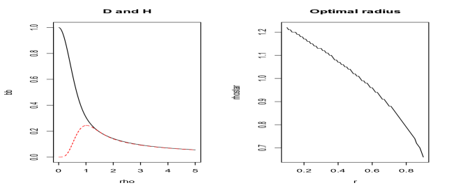
Figure 4.2: The functions $D(\rho)$ (solid line) and $H_{\rho}(r)$ (dashed line) for $r=1/2$ (left plot) and the optimal radius $\rho_{r}^{\ast}$ (right plot), both for $R(t)=e^{-t^{2}}$

For the same covariance function $R(t)=e^{-t^{2}}$ and $r=1/2$ the plots of Fig. 4.3 show the limiting shapes of the random field described in Theorem 3.3. The left plot corresponds to the sphere of radius $\rho=1$ (falling in the second case of the theorem), while the right plot correspond to the sphere of radius $\rho=2$ (falling in the first case of the theorem). Note that, by the isometry of the random field, the limiting shape is rotationally invariant. The plots, therefore, present a section of the limiting shape along the half-axis $t_{1}\geq 0,\,t_{2}=0$. For ease of comparison, the horizontal axis has been labeled in the units of $t_{1}/\rho$, i.e. relative to the radius of the sphere.

Figure 4.3: The limiting shapes for $\rho=1$ (left plot) and $\rho=2$ (right plot), both for $r=1/2$ and $R(t)=e^{-t^{2}}$

We finish this section by considering the probability $\Psi_{\text{s}p}(u;r)$ in (1.2). In this case, by (2.12) and isotropy,

$$D_{{\mathcal{C}}}(r)=\min_{0\leq b\leq 1}\min_{0\leq\rho\leq D}M_{\rho}(r;b)\,,$$ (4.58)

where $D$ is as in (4.46), and $M_{\rho}(r;b)=D_{K_{1},K_{2}}(r)$ in (2.11) with $K_{1}$ being the sphere of radius $\rho$ centered at the origin, and $K_{2}=\{b{\bf e}_{1}\}$. Here ${\bf e}_{1}$ is the $d$-dimensional vector $(1,0,\ldots,0)$. It turns out that in many circumstances the asymptotic behavior of the probabilities $\Psi_{\text{s}p;c}(u;r)$ and $\Psi_{\text{s}p}(u;r)$ is the same, at least on the logarithmic case, and so our analysis of the former probability applies to the latter probability as well.

The following result demonstrates one case when the two probabilities are asymptotically equivalent. Assume for notational simplicity that $R(0)=1$, and use the notation $S_{1}$ in place of $S_{1}({\bf 0})$. For $\rho\geq 0$, $0\leq b\leq 1$ and $\mu\in M_{1}^{+}(S_{1})$, let

$$V(\rho,b;\mu)=$$ (4.59)

$$\frac{\int_{S_{1}}\int_{S_{1}}R\bigl{(}\rho\|{\bf t}_{1}-{\bf t}_{2}\|\bigr{)}\,\mu(d{\bf t}_{1})\mu(d{\bf t}_{2})-\left(\int_{S_{1}}R(\rho\|{\bf t}-b{\bf e}_{1}\|)\,\mu(d{\bf t})\right)^{2}}{1-2r\int_{S_{1}}R(\rho\|{\bf t}-b{\bf e}_{1}\|)\,\mu(d{\bf t})+r^{2}\int_{S_{1}}\int_{S_{1}}R\bigl{(}\rho\|{\bf t}_{1}-{\bf t}_{2}\|\bigr{)}\,\mu(d{\bf t}_{1})\mu(d{\bf t}_{2})}.$$

Theorem 4.3.

Let

$$V_{*}(\rho,b)=\min_{\mu\in M_{1}^{+}\bigl{(}S_{1}\bigr{)}}V(\rho,b;\mu)$$

subject to

$$\int_{S_{1}}R(\rho\|{\bf t}-b{\bf e}_{1}\|)\,\mu(d{\bf t})\geq r\int_{S_{1}}\int_{S_{1}}R\bigl{(}\rho\|{\bf t}_{1}-{\bf t}_{2}\|\bigr{)}\,\mu(d{\bf t}_{1})\mu(d{\bf t}_{2})\,.$$ (4.60)

If, for every $0\leq\rho\leq D$ such that $R(\rho)\geq rD(\rho)$, the function $V_{*}(\rho,b),\,0\leq b\leq 1$ achieves its maximum at $b=0$, then

$$\lim_{u\to\infty}\frac{1}{u^{2}}\log\Psi_{\text{s}p}(u;r)=-\frac{1}{2}\min_{0\leq\rho\leq D}\bigl{(}W_{\rho}(r)\bigr{)}^{-1}\,,$$ (4.61)

where $W_{\rho}(r)$ is defined by (4.48).

Proof.

It follows from (4.58), (4.45) and Theorem 2.3 that we only need to check that $M_{\rho}(r)=\inf_{0\leq b\leq 1}M_{\rho}(r;b)$ for all $0\leq\rho\leq D$. Notice that by (3.30), (3.31) and isotropy,

$$M_{\rho}(r;b)=\left(\min\bigl{(}D(\rho),V_{*}(\rho,b)\bigr{)}\right)^{-1}\,,$$

where $D(\rho)$ is given in (4.49). Further, $M_{\rho}(r)=M_{\rho}(r;0)$. If $R(\rho)<rD(\rho)$, then $V_{*}(\rho,0)=\infty$, so there nothing to check. If, on the other hand, $R(\rho)\geq rD(\rho)$, then $V_{*}(\rho,\cdot)$ achieves its maximum at the origin, so the claim of the theorem follows. ∎

The condition

$$V_{*}(\rho,0)=\max_{0\leq b\leq 1}V_{*}(\rho,b)\,,$$ (4.62)

for $0\leq\rho\leq D$ such that $R(\rho)\geq rD(\rho)$, deserves a discussion. We claim that this condition is implied by the following, simpler, condition.

$$\min_{0\leq b\leq 1}\int_{S_{1}}R(\rho\|{\bf t}-b{\bf e}_{1}\|)\,\mu_{h}(d{\bf t})=\int_{S_{1}}R(\rho\|{\bf t}\|)\,\mu_{h}(d{\bf t})=R(\rho)\,,$$ (4.63)

where $\mu_{h}$ is the rotation invariant probability measure on $S_{1}$.

To see this let $R(\rho)\geq rD(\rho)$. It follows by (4.63) that the constraint (3.31) is satisfied for the measure $\mu_{h}$ and the vector $b{\bf e}_{1}$ for any $0\leq b\leq 1$. Therefore,

$$V_{*}(\rho,b)\leq V(\rho,b;\mu_{h})=G\left(\int_{S_{1}}R(\rho\|{\bf t}-b{\bf e}_{1}\|)\,\mu_{h}(d{\bf t})\right)\,,$$

where

$$G(x)=\frac{D(\rho)-x^{2}}{1-2rx+r^{2}D(\rho)},\,\ R(\rho)\leq x\leq 1\,.$$

Notice that

$$G^{\prime}(x)=\frac{-2(x-rD(\rho))(1-rx)}{\bigl{(}1-2rx+r^{2}D(\rho)\bigr{)}^{2}}\leq 0\,,$$

so that the function $G$ achieves its maximum at $x=R(\rho)$. We conclude that

$$V_{*}(\rho,b)\leq V(\rho,0;\mu_{h})=V_{*}(\rho,0)\,,$$

so that (4.62) holds.

Numerical experiments indicate that the condition (4.63) tends to hold for values of the radius $\rho$ exceeding a certain positive threshold. For instance, in dimension $d=2$ for both $R(t)=e^{-t^{2}}$ and $R(t)=e^{-|t|}$, this threshold is around $\rho=1.18$.

However, it is clear that condition (4.63) is not necessary for condition (4.62). In fact, for condition (4.62) to be satisfied one only needs a measure $\mu\in M_{1}^{+}\bigl{(}S_{1}\bigr{)}$ satisfying (4.60) such that

$$V(\rho,b;\mu)\leq V(\rho,0;\mu_{h})\,,$$ (4.64)

and what condition (4.63) guarantees is that this measure can be taken to be the rotationally invariant measure on $S_{1}$. If (4.63) fails, then there is no guarantee that the rotationally invariant measure will play the required role.

At least in the case when the covariance function $R$ is monotone, one can consider a measure $\mu$ that puts a point mass at the point on the sphere closest to the point $b{\bf e}_{1}$. We have considered measures $\mu\in M_{1}^{+}\bigl{(}S_{1}\bigr{)}$ of the form

$$\mu=w\delta_{{\rm sign}(b){\bf e}_{1}}+(1-w)\mu_{h}$$ (4.65)

for some $0\leq w\leq 1$, where $\delta_{a}$ is, as usual, the Dirac point mass at a point $a$. With this choice, the function $V$ in (4.59) becomes the ratio of two quadratic functions of $w$, and one can choose the value of $w$ that minimizes the expression, because (4.64) requires us to search for as small $V$ as possible.

In our numerical experiments we have followed an even simpler procedure and chosen the value of $w$ that minimizes the quadratic polynomial in the numerator of (4.59). For the cases of $R(t)=e^{-t^{2}}$ and $R(t)=e^{-|t|}$ the resulting measure $\mu$ in (4.65) satisfied, for all $0\leq\rho\leq D$ such that $R(\rho)\geq rD(\rho)$, both (4.60) and (4.64). Therefore, in all of these cases the conclusion (4.61) of Theorem 4.3 holds.

Acknowledgement We are indebted to Jim Renegar of Cornell University for useful discussions of the duality gap in convex optimization and for drawing our attention to the paper Anderson (1983).

References

Adler et al. (2014)R. Adler, E. Moldavskaya and G. Samorodnitsky (2014): On the
existence of paths between points in high level excursion sets of Gaussian
random fields.
Annals of Probability 42:1020–1053.
Adler and Taylor (2007)R. Adler and J. Taylor (2007): Random Fields and Geometry.
Springer, New York.
Anderson (1983)E. Anderson (1983): A review of duality theory for linear programming
over topological vector spaces.
Journal of Mathematical Analysis and Applications
97:380–392.
Azaïs and Wschebor (2009)J. Azaïs and M. Wschebor (2009): Level Sets and Extrema of
Random Processes and Fields.
Wiley, Hoboken, N.J.
Deuschel and Stroock (1989)J.-D. Deuschel and D. Stroock (1989): Large Deviations.
Academic Press, Boston.
Dunford and Schwartz (1988)N. Dunford and J. Schwartz (1988): Linear Operators, Part 1:
General Theory.
Wiley, New York.
Luenberger (1969)D. Luenberger (1969): Optimization by Vector Space Methods.
Wiley and Sons, Inc., New York.
Molchanov and Zuyev (2004)I. Molchanov and S. Zuyev (2004): Optimization in the space of
measures and optimal design.
ESAIM: Probability and Statistics 8:12–24.
Resnick (2007)S. Resnick (2007): Heavy-Tail Phenomena: Probabilistic and
Statistical Modeling.
Springer, New York.
van der Vaart and van Zanten (2008)A. van der Vaart and J. van Zanten (2008): Reproducing kernel
Hilbert spaces of Gaussian priors.
In Pushing the Limits of Contemporary Statistics: Contributions
in Honor of Jayanta K. Ghosh, volume 3 of IMS Collections.
Institute of Mathematical Statistics, pp. 200–222.