Some remarks on the use of effective Lagrangians in QED and QCD
Walter Dittrich
0.2 Compendium of Useful Formulae[DR85 ]
We start with the Green’s function of a spin-1 2 1 2 \tfrac{1}{2}
[ γ μ ( 1 i ∂ μ − e A μ ) + m ] G + ( x , x ′ ; A ) = δ ( x − x ′ ) . delimited-[] superscript 𝛾 𝜇 1 𝑖 subscript 𝜇 𝑒 subscript 𝐴 𝜇 𝑚 subscript 𝐺 𝑥 superscript 𝑥 ′ 𝐴 𝛿 𝑥 superscript 𝑥 ′ \left[\gamma^{\mu}\left(\frac{1}{i}\partial_{\mu}-eA_{\mu}\right)+m\right]G_{+}(x,x^{\prime};A)=\delta(x-x^{\prime}). (1)
If we pick a special gauge field so that F μ ν subscript 𝐹 𝜇 𝜈 F_{\mu\nu}
G + ( x , x ′ ; A ) = ϕ ( x , x ′ ) subscript 𝐺 𝑥 superscript 𝑥 ′ 𝐴 italic-ϕ 𝑥 superscript 𝑥 ′ \displaystyle G_{+}(x,x^{\prime};A)=\phi(x,x^{\prime}) ∫ 0 ∞ 1 s 2 [ m − 1 2 γ μ { f ( s ) + e F } μ ν ( x − x ′ ) ν ] superscript subscript 0 1 superscript 𝑠 2 delimited-[] 𝑚 1 2 superscript 𝛾 𝜇 subscript 𝑓 𝑠 𝑒 𝐹 𝜇 𝜈 superscript 𝑥 superscript 𝑥 ′ 𝜈 \displaystyle\int_{0}^{\infty}\frac{1}{s^{2}}\left[m-\frac{1}{2}\gamma^{\mu}\left\{f(s)+eF\right\}_{\mu\nu}(x-x^{\prime})^{\nu}\right]
× e − i m 2 s − L ( s ) + i 4 ( x − x ′ ) f ( s ) ( x − x ′ ) e i 2 σ F s d s , absent superscript 𝑒 𝑖 superscript 𝑚 2 𝑠 𝐿 𝑠 𝑖 4 𝑥 superscript 𝑥 ′ 𝑓 𝑠 𝑥 superscript 𝑥 ′ superscript 𝑒 𝑖 2 𝜎 𝐹 𝑠 𝑑 𝑠 \displaystyle\times e^{-im^{2}s-L(s)+\frac{i}{4}(x-x^{\prime})f(s)(x-x^{\prime})}e^{\frac{i}{2}\sigma Fs}ds\quad, with
f ( s ) 𝑓 𝑠 \displaystyle f(s) = e F coth ( e F s ) absent 𝑒 𝐹 hyperbolic-cotangent 𝑒 𝐹 𝑠 \displaystyle=eF\coth(eFs)
L ( s ) 𝐿 𝑠 \displaystyle L(s) = 1 2 tr ln [ sinh ( e F s ) e F s ] , absent 1 2 tr 𝑒 𝐹 𝑠 𝑒 𝐹 𝑠 \displaystyle=\frac{1}{2}\text{tr}\ln\left[\frac{\sinh(eFs)}{eFs}\right]\ ,
and ϕ ( x , x ′ ) = e i e ∫ x ′ x A μ ( ξ ) 𝑑 ξ μ italic-ϕ 𝑥 superscript 𝑥 ′ superscript 𝑒 𝑖 𝑒 superscript subscript superscript 𝑥 ′ 𝑥 superscript 𝐴 𝜇 𝜉 differential-d subscript 𝜉 𝜇 \phi(x,x^{\prime})=e^{ie\int_{x^{\prime}}^{x}A^{\mu}(\xi)d\xi_{\mu}} x 𝑥 x x ′ superscript 𝑥 ′ x^{\prime}
Our central subject of interest is the vacuum amplitude in the presence of an external field which,
in the framework of a one-loop approximation for the effective Lagrangian, can be written as
⟨ 0 + | 0 − ⟩ A superscript inner-product subscript 0 subscript 0 𝐴 \displaystyle\langle 0_{+}|0_{-}\rangle^{A} = e i W ( 1 ) [ A ] = e i ∫ ℒ ( 1 ) ( x ) d 4 x , absent superscript 𝑒 𝑖 superscript 𝑊 1 delimited-[] 𝐴 superscript 𝑒 𝑖 superscript ℒ 1 𝑥 superscript 𝑑 4 𝑥 \displaystyle=e^{iW^{(1)}\left[A\right]}=e^{i\int\mathscr{L}^{(1)}(x)d^{4}x}\quad, (2) with
i W ( 1 ) [ A ] 𝑖 superscript 𝑊 1 delimited-[] 𝐴 \displaystyle iW^{(1)}\left[A\right] = − Tr ln ( 1 1 − e γ A G + ) = − Tr ln ( G + [ A ] G + [ 0 ] ) . absent Tr 1 1 𝑒 𝛾 𝐴 subscript 𝐺 Tr subscript 𝐺 delimited-[] 𝐴 subscript 𝐺 delimited-[] 0 \displaystyle=-\text{Tr}\ln\left(\frac{1}{1-e\gamma AG_{+}}\right)=-\text{Tr}\ln\left(\frac{G_{+}\left[A\right]}{G_{+}\left[0\right]}\right)\ . (3)
Here G + = G + [ 0 ] subscript 𝐺 subscript 𝐺 delimited-[] 0 G_{+}=G_{+}[0] G + [ A ] subscript 𝐺 delimited-[] 𝐴 G_{+}[A]
G + [ A ] = G + ( 1 − e γ A G + ) − 1 . subscript 𝐺 delimited-[] 𝐴 subscript 𝐺 superscript 1 𝑒 𝛾 𝐴 subscript 𝐺 1 G_{+}[A]=G_{+}(1-e\gamma AG_{+})^{-1}\quad. (4)
Furthermore, Tr indicates the trace both in spinor and configuration space.
The one-loop effective action W ( 1 ) superscript 𝑊 1 W^{(1)} ℒ ( 1 ) superscript ℒ 1 \mathscr{L}^{(1)}
The functional derivative with respect to the potential A μ ( x ) subscript 𝐴 𝜇 𝑥 A_{\mu}(x)
i δ W ( 1 ) [ A ] δ A μ ( x ) = − e tr [ γ μ G + ( x , x ; A ) ] . 𝑖 𝛿 superscript 𝑊 1 delimited-[] 𝐴 𝛿 subscript 𝐴 𝜇 𝑥 𝑒 tr delimited-[] superscript 𝛾 𝜇 subscript 𝐺 𝑥 𝑥 𝐴 i\frac{\delta W^{(1)}[A]}{\delta A_{\mu}(x)}=-e\text{tr}\left[\gamma^{\mu}G_{+}(x,x;A)\right]\quad. (5)
This equation is fulfilled by the ansatz
i W ( 1 ) := i ∫ ℒ ( 1 ) d 4 x = − 1 2 ∫ 0 ∞ e − i s m 2 s Tr [ e i s ( γ ⋅ Π ) 2 ] 𝑑 s , assign 𝑖 superscript 𝑊 1 𝑖 superscript ℒ 1 superscript 𝑑 4 𝑥 1 2 superscript subscript 0 superscript 𝑒 𝑖 𝑠 superscript 𝑚 2 𝑠 Tr delimited-[] superscript 𝑒 𝑖 𝑠 superscript ⋅ 𝛾 Π 2 differential-d 𝑠 iW^{(1)}:=i\int\mathscr{L}^{(1)}d^{4}x=-\frac{1}{2}\int_{0}^{\infty}\frac{e^{-ism^{2}}}{s}\text{Tr}\left[e^{is(\gamma\cdot\Pi)^{2}}\right]ds\ , (6)
where the proper-time representation of G + [ A ] subscript 𝐺 delimited-[] 𝐴 G_{+}[A]
G + [ A ] ⋅ γ ⋅ Π − m ( γ ⋅ Π ) 2 − m 2 = ( m − γ ⋅ Π ) i ∫ 0 ∞ e − i s [ m 2 − ( γ ⋅ Π ) 2 ] 𝑑 s . ⋅ subscript 𝐺 delimited-[] 𝐴 ⋅ 𝛾 Π 𝑚 superscript ⋅ 𝛾 Π 2 superscript 𝑚 2 𝑚 ⋅ 𝛾 Π 𝑖 superscript subscript 0 superscript 𝑒 𝑖 𝑠 delimited-[] superscript 𝑚 2 superscript ⋅ 𝛾 Π 2 differential-d 𝑠 G_{+}[A]\cdot\frac{\gamma\cdot\Pi-m}{(\gamma\cdot\Pi)^{2}-m^{2}}=(m-\gamma\cdot\Pi)i\int_{0}^{\infty}e^{-is\left[m^{2}-(\gamma\cdot\Pi)^{2}\right]}ds\quad. (7)
We can then write for the unrenormalized Lagrangian
ℒ ( 1 ) ( x ) = i 2 tr ∫ 0 ∞ e − i m 2 s s ⟨ x | e i s ( γ ⋅ Π ) 2 | x ⟩ 𝑑 s , superscript ℒ 1 𝑥 𝑖 2 tr superscript subscript 0 superscript 𝑒 𝑖 superscript 𝑚 2 𝑠 𝑠 quantum-operator-product 𝑥 superscript 𝑒 𝑖 𝑠 superscript ⋅ 𝛾 Π 2 𝑥 differential-d 𝑠 \mathscr{L}^{(1)}(x)=\frac{i}{2}\text{tr}\int_{0}^{\infty}\frac{e^{-im^{2}s}}{s}\langle x|e^{is(\gamma\cdot\Pi)^{2}}|x\rangle ds\ , (8)
where the trace refers only to the spinor index.
With this expression for ℒ ( 1 ) ( x ) superscript ℒ 1 𝑥 \mathscr{L}^{(1)}(x)
i ∂ ℒ ( 1 ) ∂ m = tr G + ( x , x ; A ) . 𝑖 superscript ℒ 1 𝑚 tr subscript 𝐺 𝑥 𝑥 𝐴 i\frac{\partial\mathscr{L}^{(1)}}{\partial m}=\text{tr}\ G_{+}(x,x;A)\ . (9)
Without further proof we also find for the trace of the energy-momentum tensor
⟨ T μ μ ( x ) ⟩ = − i m tr G + ( x , x ; A ) . delimited-⟨⟩ superscript subscript 𝑇 𝜇 𝜇 𝑥 𝑖 𝑚 tr subscript 𝐺 𝑥 𝑥 𝐴 \langle T_{\mu}^{\mu}(x)\rangle=-im\ \text{tr}\ G_{+}(x,x;A)\ . (10)
This leads us to the equation
⟨ T μ μ ( x ) ⟩ delimited-⟨⟩ superscript subscript 𝑇 𝜇 𝜇 𝑥 \displaystyle\langle T_{\mu}^{\mu}(x)\rangle = − i m tr ⟨ x | ( − γ ⋅ Π + m ) i ∫ 0 ∞ e − i ( m 2 − ( γ ⋅ Π ) 2 ) s 𝑑 s | x ⟩ absent 𝑖 𝑚 tr quantum-operator-product 𝑥 ⋅ 𝛾 Π 𝑚 𝑖 superscript subscript 0 superscript 𝑒 𝑖 superscript 𝑚 2 superscript ⋅ 𝛾 Π 2 𝑠 differential-d 𝑠 𝑥 \displaystyle=-im\text{tr}\langle x|(-\gamma\cdot\Pi+m)i\int_{0}^{\infty}e^{-i\left(m^{2}-(\gamma\cdot\Pi)^{2}\right)s}ds|x\rangle
= m 2 ⟨ x | tr ∫ 0 ∞ e − i ( m 2 − ( γ ⋅ Π ) 2 ) s 𝑑 s | x ⟩ . absent superscript 𝑚 2 quantum-operator-product 𝑥 tr superscript subscript 0 superscript 𝑒 𝑖 superscript 𝑚 2 superscript ⋅ 𝛾 Π 2 𝑠 differential-d 𝑠 𝑥 \displaystyle=m^{2}\langle x|\text{tr}\int_{0}^{\infty}e^{-i\left(m^{2}-(\gamma\cdot\Pi)^{2}\right)s}ds|x\rangle\ .
With the former expression for ℒ ( 1 ) superscript ℒ 1 \mathscr{L}^{(1)}
⟨ T μ μ ( x ) ⟩ = m ∂ ℒ ( 1 ) ( x ) ∂ m = ∂ ℒ ( 1 ) ( x ) ∂ ( ln m ) . delimited-⟨⟩ superscript subscript 𝑇 𝜇 𝜇 𝑥 𝑚 superscript ℒ 1 𝑥 𝑚 superscript ℒ 1 𝑥 𝑚 \langle T_{\mu}^{\mu}(x)\rangle=m\frac{\partial\mathscr{L}^{(1)}(x)}{\partial m}=\frac{\partial\mathscr{L}^{(1)}(x)}{\partial(\ln m)}\quad. (11)
For a purely constant magnetic field the renormalized one-loop effective Lagrangian is known to be
ℒ ( 1 ) ( H ) = − 1 8 π 2 ∫ 0 ∞ e − m 2 s s 2 [ ( e H s ) coth ( e H s ) − 1 3 ( e H s ) 2 − 1 ] 𝑑 s . superscript ℒ 1 𝐻 1 8 superscript 𝜋 2 superscript subscript 0 superscript 𝑒 superscript 𝑚 2 𝑠 superscript 𝑠 2 delimited-[] 𝑒 𝐻 𝑠 hyperbolic-cotangent 𝑒 𝐻 𝑠 1 3 superscript 𝑒 𝐻 𝑠 2 1 differential-d 𝑠 \mathscr{L}^{(1)}(H)=-\frac{1}{8\pi^{2}}\int_{0}^{\infty}\frac{e^{-m^{2}s}}{s^{2}}\left[(eHs)\coth(eHs)-\frac{1}{3}(eHs)^{2}-1\right]ds\ . (12)
The integral can be explicitly calculated by dimensional or ζ 𝜁 \zeta ℒ ( 1 ) ( H ) superscript ℒ 1 𝐻 \mathscr{L}^{(1)}(H)
0.3 The trace anomaly of the energy-momentum tensor from the one-loop effective Lagrangian in QED
We already mentioned the close connection between the effective Lagrangian ℒ ( 1 ) superscript ℒ 1 \mathscr{L}^{(1)}
⟨ T μ μ ( x ) ⟩ = m ∂ ℒ ( 1 ) ( x ) ∂ m . delimited-⟨⟩ superscript subscript 𝑇 𝜇 𝜇 𝑥 𝑚 superscript ℒ 1 𝑥 𝑚 \langle T_{\mu}^{\mu}(x)\rangle=m\frac{\partial\mathscr{L}^{(1)}(x)}{\partial m}\ . (13)
For constant fields we have the expression
⟨ T μ μ ( x ) ⟩ ( ℱ , 𝒢 ) delimited-⟨⟩ superscript subscript 𝑇 𝜇 𝜇 𝑥 ℱ 𝒢 \displaystyle\langle T_{\mu}^{\mu}(x)\rangle\left(\mathcal{F},\mathcal{G}\right) = m 2 16 π 2 4 ∫ 0 ∞ e − m 2 s s 2 [ e 2 s 2 𝒢 ℜ 𝔢 cosh ( e s 2 ( ℱ + i 𝒢 ) 1 / 2 ) ℑ 𝔪 cosh ( e s 2 ( ℱ + i 𝒢 ) 1 / 2 ) \displaystyle=\frac{m^{2}}{16\pi^{2}}4\int_{0}^{\infty}\frac{e^{-m^{2}s}}{s^{2}}\left[e^{2}s^{2}\mathcal{G}\frac{\mathfrak{Re}\cosh\left(es\sqrt{2}(\mathcal{F}+i\mathcal{G})^{1/2}\right)}{\mathfrak{Im}\cosh\left(es\sqrt{2}(\mathcal{F}+i\mathcal{G})^{1/2}\right)}\right.
− 1 − 2 3 e 2 s 2 ℱ ] d s , \displaystyle\left.-1-\frac{2}{3}e^{2}s^{2}\mathcal{F}\right]ds\quad, where
ℱ ℱ \displaystyle\mathcal{F} = 1 4 F μ ν F μ ν = 1 2 ( H 2 − E 2 ) , absent 1 4 subscript 𝐹 𝜇 𝜈 superscript 𝐹 𝜇 𝜈 1 2 superscript 𝐻 2 superscript 𝐸 2 \displaystyle=\frac{1}{4}F_{\mu\nu}F^{\mu\nu}=\frac{1}{2}\left(H^{2}-E^{2}\right)\ ,
𝒢 𝒢 \displaystyle\mathcal{G} = 1 4 F μ ν F μ ν = E → ⋅ H → , absent 1 4 superscript 𝐹 𝜇 𝜈 subscript 𝐹 𝜇 𝜈 ⋅ → 𝐸 → 𝐻 \displaystyle=\frac{1}{4}F^{\mu\nu}F_{\mu\nu}=\vec{E}\cdot\vec{H}\quad, with
F μ ν subscript 𝐹 𝜇 𝜈 \displaystyle F_{\mu\nu} = 1 2 ϵ μ ν κ λ F κ λ , ϵ 0123 = 1 . formulae-sequence absent 1 2 subscript italic-ϵ 𝜇 𝜈 𝜅 𝜆 superscript 𝐹 𝜅 𝜆 subscript italic-ϵ 0123 1 \displaystyle=\frac{1}{2}\epsilon_{\mu\nu\kappa\lambda}F^{\kappa\lambda},\quad\epsilon_{0123}=1\ .
The closed-form expression ℒ ( 1 ) superscript ℒ 1 \mathscr{L}^{(1)} H 𝐻 H
ℒ ( 1 ) ( H ) superscript ℒ 1 𝐻 \displaystyle\mathscr{L}^{(1)}(H) = − 1 32 π 2 [ ( 2 m 4 − 4 m 2 ( e H ) + 4 3 ( e H ) 2 ) [ 1 + ln ( m 2 2 e H ) ] \displaystyle=-\frac{1}{32\pi^{2}}\left[(2m^{4}-4m^{2}(eH)+\frac{4}{3}(eH)^{2})\left[1+\ln\left(\frac{m^{2}}{2eH}\right)\right]\right.
+ 4 m 2 ( e H ) − 3 m 4 − ( 4 e H ) 2 ζ ′ ( − 1 , m 2 2 e H ) ] . \displaystyle\left.+4m^{2}(eH)-3m^{4}-(4eH)^{2}\zeta^{\prime}\left(-1,\frac{m^{2}}{2eH}\right)\right]\quad.
The result of the mass-differentiation turns out to be
⟨ T μ μ ⟩ ( H ) delimited-⟨⟩ superscript subscript 𝑇 𝜇 𝜇 𝐻 \displaystyle\langle T_{\mu}^{\mu}\rangle(H) = − 1 12 π 2 ( e H ) 2 − m 4 4 π 2 ln ( m 2 2 e H ) + m 2 4 π 2 ( e H ) ln ( m 2 2 e H ) absent 1 12 superscript 𝜋 2 superscript 𝑒 𝐻 2 superscript 𝑚 4 4 superscript 𝜋 2 superscript 𝑚 2 2 𝑒 𝐻 superscript 𝑚 2 4 superscript 𝜋 2 𝑒 𝐻 superscript 𝑚 2 2 𝑒 𝐻 \displaystyle=-\frac{1}{12\pi^{2}}(eH)^{2}-\frac{m^{4}}{4\pi^{2}}\ln\left(\frac{m^{2}}{2eH}\right)+\frac{m^{2}}{4\pi^{2}}(eH)\ln\left(\frac{m^{2}}{2eH}\right)
+ m 4 4 π 2 + ( e H ) m 2 2 π 2 [ ln Γ ( m 2 2 e H ) − 1 2 ln 2 π ] . superscript 𝑚 4 4 superscript 𝜋 2 𝑒 𝐻 superscript 𝑚 2 2 superscript 𝜋 2 delimited-[] Γ superscript 𝑚 2 2 𝑒 𝐻 1 2 2 𝜋 \displaystyle+\frac{m^{4}}{4\pi^{2}}+\frac{(eH)m^{2}}{2\pi^{2}}\left[\ln\Gamma\left(\frac{m^{2}}{2eH}\right)-\frac{1}{2}\ln 2\pi\right]\quad.
This, by the way, is also the result of the calculation of the integral
⟨ T μ μ ⟩ ( H ) = − i e H m 2 4 π 2 ∫ 0 ∞ e − 2 i h z z 2 [ z cot z − 1 + 1 3 z 2 ] 𝑑 z , h = m 2 2 e H . formulae-sequence delimited-⟨⟩ superscript subscript 𝑇 𝜇 𝜇 𝐻 𝑖 𝑒 𝐻 superscript 𝑚 2 4 superscript 𝜋 2 superscript subscript 0 superscript 𝑒 2 𝑖 ℎ 𝑧 superscript 𝑧 2 delimited-[] 𝑧 𝑧 1 1 3 superscript 𝑧 2 differential-d 𝑧 ℎ superscript 𝑚 2 2 𝑒 𝐻 \langle T_{\mu}^{\mu}\rangle(H)=-i\frac{eHm^{2}}{4\pi^{2}}\int_{0}^{\infty}\frac{e^{-2ihz}}{z^{2}}\left[z\cot z-1+\frac{1}{3}z^{2}\right]dz,\quad h=\frac{m^{2}}{2eH}\ . (14)
Now observe that for h ≪ 1 much-less-than ℎ 1 h\ll 1 ln Γ ( h ) ≈ − ln h Γ ℎ ℎ \ln\Gamma(h)\approx-\ln h
lim m → 0 ⟨ T μ μ ⟩ ( H ) = − 1 12 π 2 e 2 H 2 , subscript → 𝑚 0 delimited-⟨⟩ superscript subscript 𝑇 𝜇 𝜇 𝐻 1 12 superscript 𝜋 2 superscript 𝑒 2 superscript 𝐻 2 \lim_{m\rightarrow 0}\langle T_{\mu}^{\mu}\rangle(H)=-\frac{1}{12\pi^{2}}e^{2}H^{2}\ , (15)
which, when written covariantly, yields
m → 0 : ⟨ T μ μ ⟩ = − 1 24 π 2 e 2 F μ ν F μ ν = − 2 α 3 π 1 4 F μ ν F μ ν . m\rightarrow 0\ :\quad\langle T_{\mu}^{\mu}\rangle=-\frac{1}{24\pi^{2}}e^{2}F_{\mu\nu}F^{\mu\nu}=-\frac{2\alpha}{3\pi}\frac{1}{4}F_{\mu\nu}F^{\mu\nu}\ . (16)
We can also obtain the next-to-leading term,
⟨ T μ μ ⟩ = − β ( α ) 1 4 F μ ν F μ ν , β ( α ) = 2 3 ( α π ) + 1 2 ( α π ) 2 , formulae-sequence delimited-⟨⟩ superscript subscript 𝑇 𝜇 𝜇 𝛽 𝛼 1 4 subscript 𝐹 𝜇 𝜈 superscript 𝐹 𝜇 𝜈 𝛽 𝛼 2 3 𝛼 𝜋 1 2 superscript 𝛼 𝜋 2 \langle T_{\mu}^{\mu}\rangle=-\beta(\alpha)\frac{1}{4}F_{\mu\nu}F^{\mu\nu},\quad\beta(\alpha)=\frac{2}{3}\left(\frac{\alpha}{\pi}\right)+\frac{1}{2}\left(\frac{\alpha}{\pi}\right)^{2}\ , (17)
by incorporating results for the two-loop calculation ℒ ( 2 ) superscript ℒ 2 \mathscr{L}^{(2)}
For large field strengths, e H m 2 ≫ 1 much-greater-than 𝑒 𝐻 superscript 𝑚 2 1 \frac{eH}{m^{2}}\gg 1
⟨ T μ μ ⟩ ( H ) = − α 3 π H 2 , delimited-⟨⟩ superscript subscript 𝑇 𝜇 𝜇 𝐻 𝛼 3 𝜋 superscript 𝐻 2 \langle T_{\mu}^{\mu}\rangle(H)=-\frac{\alpha}{3\pi}H^{2}\ , (18)
while for small field strength, e H m 2 ≪ 1 much-less-than 𝑒 𝐻 superscript 𝑚 2 1 \frac{eH}{m^{2}}\ll 1 Γ Γ \Gamma
⟨ T μ μ ⟩ ( H ) = 4 ( − 2 α 2 45 H 4 m 4 + 64 315 π α 3 H 6 m 8 + … ) . delimited-⟨⟩ superscript subscript 𝑇 𝜇 𝜇 𝐻 4 2 superscript 𝛼 2 45 superscript 𝐻 4 superscript 𝑚 4 64 315 𝜋 superscript 𝛼 3 superscript 𝐻 6 superscript 𝑚 8 … \langle T_{\mu}^{\mu}\rangle(H)=4\left(-\frac{2\alpha^{2}}{45}\frac{H^{4}}{m^{4}}+\frac{64}{315}\pi\alpha^{3}\frac{H^{6}}{m^{8}}+\dots\right)\ . (19)
Interestingly, the first term in this expansion agrees with Schwinger’s[Sch51 ] from the Heisenberg-Euler Lagrangian:
T μ ν = T μ ν M a x w e l l ( 1 − 16 45 α 2 1 m 4 ℱ ) − δ μ ν 2 45 α 2 1 m 4 ( 4 ℱ 2 + ℱ 𝒢 2 ) . subscript 𝑇 𝜇 𝜈 superscript subscript 𝑇 𝜇 𝜈 𝑀 𝑎 𝑥 𝑤 𝑒 𝑙 𝑙 1 16 45 superscript 𝛼 2 1 superscript 𝑚 4 ℱ subscript 𝛿 𝜇 𝜈 2 45 superscript 𝛼 2 1 superscript 𝑚 4 4 superscript ℱ 2 ℱ superscript 𝒢 2 T_{\mu\nu}=T_{\mu\nu}^{Maxwell}\left(1-\frac{16}{45}\alpha^{2}\frac{1}{m^{4}}\mathcal{F}\right)-\delta_{\mu\nu}\frac{2}{45}\alpha^{2}\frac{1}{m^{4}}\left(4\mathcal{F}^{2}+\mathcal{F}\mathcal{G}^{2}\right)\ . (20)
In our present case we use ℏ = c = 1 Planck-constant-over-2-pi 𝑐 1 \hbar=c=1 E → = 0 → → 𝐸 → 0 \vec{E}=\vec{0} ℱ = 1 2 ( H 2 − E 2 ) = 1 2 H 2 ℱ 1 2 superscript 𝐻 2 superscript 𝐸 2 1 2 superscript 𝐻 2 \mathcal{F}=\tfrac{1}{2}(H^{2}-E^{2})=\tfrac{1}{2}H^{2} 𝒢 = E → ⋅ H → = 0 𝒢 ⋅ → 𝐸 → 𝐻 0 \mathcal{G}=\vec{E}\cdot\vec{H}=0
Since we are interested in the trace of T μ ν subscript 𝑇 𝜇 𝜈 T_{\mu\nu}
⟨ T μ μ ⟩ delimited-⟨⟩ subscript 𝑇 𝜇 𝜇 \displaystyle\langle T_{\mu\mu}\rangle = − 4 ( 8 α 2 45 m 4 ℱ 2 + 14 α 2 45 m 4 𝒢 2 ) , absent 4 8 superscript 𝛼 2 45 superscript 𝑚 4 superscript ℱ 2 14 superscript 𝛼 2 45 superscript 𝑚 4 superscript 𝒢 2 \displaystyle=-4\left(\frac{8\alpha^{2}}{45m^{4}}\mathcal{F}^{2}+\frac{14\alpha^{2}}{45m^{4}}\mathcal{G}^{2}\right)\ , which for 𝒢 = 0 𝒢 0 \mathcal{G}=0
⟨ T μ μ ⟩ ( H ) delimited-⟨⟩ subscript 𝑇 𝜇 𝜇 𝐻 \displaystyle\langle T_{\mu\mu}\rangle(H) = − 4 ( 2 α 2 45 H 4 m 4 ) . absent 4 2 superscript 𝛼 2 45 superscript 𝐻 4 superscript 𝑚 4 \displaystyle=-4\left(\frac{2\alpha^{2}}{45}\frac{H^{4}}{m^{4}}\right)\ .
Let us prove Schwinger’s formula. He starts with
T μ ν = δ μ ν ℒ − 2 ∂ ℒ ∂ F μ λ F ν λ . subscript 𝑇 𝜇 𝜈 subscript 𝛿 𝜇 𝜈 ℒ 2 ℒ subscript 𝐹 𝜇 𝜆 subscript 𝐹 𝜈 𝜆 T_{\mu\nu}=\delta_{\mu\nu}\mathscr{L}-2\frac{\partial\mathscr{L}}{\partial F_{\mu\lambda}}F_{\nu\lambda}\ . (21)
(Note that in Schwinger’s formula the factor 2 2 2
We need the following derivatives:
∂ ℒ ( ℱ , 𝒢 ) ∂ F μ λ ℒ ℱ 𝒢 subscript 𝐹 𝜇 𝜆 \displaystyle\frac{\partial\mathscr{L}(\mathcal{F},\mathcal{G})}{\partial F_{\mu\lambda}} = ∂ ℒ ∂ ℱ ∂ ℱ ∂ F μ λ + ∂ ℒ ∂ 𝒢 ∂ 𝒢 ∂ F μ λ , absent ℒ ℱ ℱ subscript 𝐹 𝜇 𝜆 ℒ 𝒢 𝒢 subscript 𝐹 𝜇 𝜆 \displaystyle=\frac{\partial\mathscr{L}}{\partial\mathcal{F}}\frac{\partial\mathcal{F}}{\partial F_{\mu\lambda}}+\frac{\partial\mathscr{L}}{\partial\mathcal{G}}\frac{\partial\mathcal{G}}{\partial F_{\mu\lambda}},
∂ ℱ ∂ F μ λ ℱ subscript 𝐹 𝜇 𝜆 \displaystyle\frac{\partial\mathcal{F}}{\partial F_{\mu\lambda}} = ∂ ∂ F μ λ ( 1 4 F ρ σ 2 ) = 1 2 F μ λ absent subscript 𝐹 𝜇 𝜆 1 4 subscript superscript 𝐹 2 𝜌 𝜎 1 2 subscript 𝐹 𝜇 𝜆 \displaystyle=\frac{\partial}{\partial F_{\mu\lambda}}\left(\frac{1}{4}F^{2}_{\rho\sigma}\right)=\frac{1}{2}F_{\mu\lambda}
∂ 𝒢 ∂ F μ λ 𝒢 subscript 𝐹 𝜇 𝜆 \displaystyle\frac{\partial\mathcal{G}}{\partial F_{\mu\lambda}} = ∂ ∂ F μ λ ( 1 4 F ρ σ F ρ σ ∗ ) = 1 4 ∂ ∂ F μ λ ( F ρ σ i 2 ϵ ρ σ τ ω F τ ω ) absent subscript 𝐹 𝜇 𝜆 1 4 subscript 𝐹 𝜌 𝜎 subscript superscript 𝐹 𝜌 𝜎 1 4 subscript 𝐹 𝜇 𝜆 subscript 𝐹 𝜌 𝜎 𝑖 2 subscript italic-ϵ 𝜌 𝜎 𝜏 𝜔 subscript 𝐹 𝜏 𝜔 \displaystyle=\frac{\partial}{\partial F_{\mu\lambda}}\left(\frac{1}{4}F_{\rho\sigma}F^{*}_{\rho\sigma}\right)=\frac{1}{4}\frac{\partial}{\partial F_{\mu\lambda}}\left(F_{\rho\sigma}\frac{i}{2}\epsilon_{\rho\sigma\tau\omega}F_{\tau\omega}\right)
= 1 2 F λ μ ∗ . absent 1 2 superscript subscript 𝐹 𝜆 𝜇 \displaystyle=\frac{1}{2}F_{\lambda\mu}^{*}\quad.
Hence we can write
∂ ℒ ( ℱ , 𝒢 ) ∂ F μ λ ℒ ℱ 𝒢 subscript 𝐹 𝜇 𝜆 \displaystyle\frac{\partial\mathscr{L}(\mathcal{F},\mathcal{G})}{\partial F_{\mu\lambda}} = ∂ ℒ ∂ ℱ 1 2 F μ λ + ∂ ℒ ∂ 𝒢 1 2 F λ μ ∗ , absent ℒ ℱ 1 2 subscript 𝐹 𝜇 𝜆 ℒ 𝒢 1 2 superscript subscript 𝐹 𝜆 𝜇 \displaystyle=\frac{\partial\mathscr{L}}{\partial\mathcal{F}}\frac{1}{2}F_{\mu\lambda}+\frac{\partial\mathscr{L}}{\partial\mathcal{G}}\frac{1}{2}F_{\lambda\mu}^{*}\ , so that
− 2 ∂ ℒ ∂ F μ λ F ν λ 2 ℒ subscript 𝐹 𝜇 𝜆 subscript 𝐹 𝜈 𝜆 \displaystyle-2\frac{\partial\mathscr{L}}{\partial F_{\mu\lambda}}F_{\nu\lambda} = − ∂ ℒ ∂ ℱ F μ λ F ν λ − ∂ ℒ ∂ 𝒢 F λ μ ∗ F ν λ ⏟ = 𝒢 δ μ ν absent ℒ ℱ subscript 𝐹 𝜇 𝜆 subscript 𝐹 𝜈 𝜆 ℒ 𝒢 subscript ⏟ superscript subscript 𝐹 𝜆 𝜇 subscript 𝐹 𝜈 𝜆 absent 𝒢 subscript 𝛿 𝜇 𝜈 \displaystyle=-\frac{\partial\mathscr{L}}{\partial\mathcal{F}}F_{\mu\lambda}F_{\nu\lambda}-\frac{\partial\mathscr{L}}{\partial\mathcal{G}}\underbrace{F_{\lambda\mu}^{*}F_{\nu\lambda}}_{=\mathcal{G}\delta_{\mu\nu}}
= − F μ λ F ν λ ∂ ℒ ∂ ℱ − δ μ ν 𝒢 ∂ ℒ ∂ 𝒢 + ( δ μ ν ℱ ∂ ℒ ∂ ℱ − δ μ ν ℱ ∂ ℒ ∂ ℱ ) . absent subscript 𝐹 𝜇 𝜆 subscript 𝐹 𝜈 𝜆 ℒ ℱ subscript 𝛿 𝜇 𝜈 𝒢 ℒ 𝒢 subscript 𝛿 𝜇 𝜈 ℱ ℒ ℱ subscript 𝛿 𝜇 𝜈 ℱ ℒ ℱ \displaystyle=-F_{\mu\lambda}F_{\nu\lambda}\frac{\partial\mathscr{L}}{\partial\mathcal{F}}-\delta_{\mu\nu}\mathcal{G}\frac{\partial\mathscr{L}}{\partial\mathcal{G}}+\left(\delta_{\mu\nu}\mathcal{F}\frac{\partial\mathscr{L}}{\partial\mathcal{F}}-\delta_{\mu\nu}\mathcal{F}\frac{\partial\mathscr{L}}{\partial\mathcal{F}}\right)\ .
Putting everything together we obtain
T μ ν subscript 𝑇 𝜇 𝜈 \displaystyle T_{\mu\nu} = − F μ λ F ν λ ∂ ℒ ∂ ℱ + δ μ ν ℱ ∂ ℒ ∂ ℱ + δ μ λ ℒ − δ μ ν ℱ ∂ ℒ ∂ ℱ − δ μ ν 𝒢 ∂ ℒ ∂ 𝒢 absent subscript 𝐹 𝜇 𝜆 subscript 𝐹 𝜈 𝜆 ℒ ℱ subscript 𝛿 𝜇 𝜈 ℱ ℒ ℱ subscript 𝛿 𝜇 𝜆 ℒ subscript 𝛿 𝜇 𝜈 ℱ ℒ ℱ subscript 𝛿 𝜇 𝜈 𝒢 ℒ 𝒢 \displaystyle=-F_{\mu\lambda}F_{\nu\lambda}\frac{\partial\mathscr{L}}{\partial\mathcal{F}}+\delta_{\mu\nu}\mathcal{F}\frac{\partial\mathscr{L}}{\partial\mathcal{F}}+\delta_{\mu\lambda}\mathscr{L}-\delta_{\mu\nu}\mathcal{F}\frac{\partial\mathscr{L}}{\partial\mathcal{F}}-\delta_{\mu\nu}\mathcal{G}\frac{\partial\mathscr{L}}{\partial\mathcal{G}}
= − ( F μ λ F ν λ − δ μ ν 1 4 F λ κ 2 ) ⏟ = T μ ν M ∂ ℒ ∂ ℱ + δ μ ν ( ℒ − ℱ ∂ ℒ ∂ ℱ − 𝒢 ∂ ℒ ∂ 𝒢 ) , absent subscript ⏟ subscript 𝐹 𝜇 𝜆 subscript 𝐹 𝜈 𝜆 subscript 𝛿 𝜇 𝜈 1 4 superscript subscript 𝐹 𝜆 𝜅 2 absent superscript subscript 𝑇 𝜇 𝜈 𝑀 ℒ ℱ subscript 𝛿 𝜇 𝜈 ℒ ℱ ℒ ℱ 𝒢 ℒ 𝒢 \displaystyle=-\underbrace{\left(F_{\mu\lambda}F_{\nu\lambda}-\delta_{\mu\nu}\frac{1}{4}F_{\lambda\kappa}^{2}\right)}_{=T_{\mu\nu}^{M}}\frac{\partial\mathscr{L}}{\partial\mathcal{F}}+\delta_{\mu\nu}\left(\mathscr{L}-\mathcal{F}\frac{\partial\mathscr{L}}{\partial\mathcal{F}}-\mathcal{G}\frac{\partial\mathscr{L}}{\partial\mathcal{G}}\right)\ ,
which is a gauge-invariant expression.
Now, from the Heisenberg-Euler effective Lagrangian we are given
ℒ = − ℱ + C [ 4 ℱ 2 + 7 𝒢 2 ] , C = 2 α 2 45 m 4 , ℏ = c = 1 . formulae-sequence ℒ ℱ 𝐶 delimited-[] 4 superscript ℱ 2 7 superscript 𝒢 2 formulae-sequence 𝐶 2 superscript 𝛼 2 45 superscript 𝑚 4 Planck-constant-over-2-pi 𝑐 1 \mathscr{L}=-\mathcal{F}+C\left[4\mathcal{F}^{2}+7\mathcal{G}^{2}\right],\ C=\frac{2\alpha^{2}}{45m^{4}},\ \hbar=c=1\ . (22)
From this expression we obtain the derivatives
∂ ℒ ∂ ℱ ℒ ℱ \displaystyle\frac{\partial\mathscr{L}}{\partial\mathcal{F}} = − 1 + 8 C ℱ , absent 1 8 𝐶 ℱ \displaystyle=-1+8C\mathcal{F}\quad, ℱ ∂ ℒ ∂ ℱ ℱ ℒ ℱ \displaystyle\mathcal{F}\frac{\partial\mathscr{L}}{\partial\mathcal{F}} = − ℱ + 8 C ℱ 2 absent ℱ 8 𝐶 superscript ℱ 2 \displaystyle=-\mathcal{F}+8C\mathcal{F}^{2}
∂ ℒ ∂ 𝒢 ℒ 𝒢 \displaystyle\frac{\partial\mathscr{L}}{\partial\mathcal{G}} = 14 C 𝒢 , absent 14 𝐶 𝒢 \displaystyle=14C\mathcal{G}\quad, 𝒢 ∂ ℒ ∂ 𝒢 𝒢 ℒ 𝒢 \displaystyle\mathcal{G}\frac{\partial\mathscr{L}}{\partial\mathcal{G}} = 14 C 𝒢 2 . absent 14 𝐶 superscript 𝒢 2 \displaystyle=14C\mathcal{G}^{2}\ .
Finally we end up with
T μ ν subscript 𝑇 𝜇 𝜈 \displaystyle T_{\mu\nu} = T μ ν M ( 1 − 16 α 2 45 m 4 ℱ ) + δ μ ν ( ℒ + ℱ − 8 C ℱ 2 − 14 C 𝒢 2 ) , ( ℒ = − ℱ + C ( 4 ℱ 2 + 7 𝒢 2 ) ) absent superscript subscript 𝑇 𝜇 𝜈 𝑀 1 16 superscript 𝛼 2 45 superscript 𝑚 4 ℱ subscript 𝛿 𝜇 𝜈 ℒ ℱ 8 𝐶 superscript ℱ 2 14 𝐶 superscript 𝒢 2 ℒ ℱ 𝐶 4 superscript ℱ 2 7 superscript 𝒢 2
\displaystyle=T_{\mu\nu}^{M}\left(1-\frac{16\alpha^{2}}{45m^{4}}\mathcal{F}\right)+\delta_{\mu\nu}\left(\mathscr{L}+\mathcal{F}-8C\mathcal{F}^{2}-14C\mathcal{G}^{2}\right),\left(\mathscr{L}=-\mathcal{F}+C(4\mathcal{F}^{2}+7\mathcal{G}^{2})\right)
= T μ ν M ( 1 − 16 α 2 45 m 4 ℱ ) − δ μ ν 2 α 2 45 m 4 ( 4 ℱ 2 + 7 𝒢 2 ) □ absent superscript subscript 𝑇 𝜇 𝜈 𝑀 1 16 superscript 𝛼 2 45 superscript 𝑚 4 ℱ subscript 𝛿 𝜇 𝜈 2 superscript 𝛼 2 45 superscript 𝑚 4 4 superscript ℱ 2 7 superscript 𝒢 2 □
\displaystyle=T_{\mu\nu}^{M}\left(1-\frac{16\alpha^{2}}{45m^{4}}\mathcal{F}\right)-\delta_{\mu\nu}\frac{2\alpha^{2}}{45m^{4}}\left(4\mathcal{F}^{2}+7\mathcal{G}^{2}\right)\qquad\square
Let us put things together. Besides ⟨ T μ μ ⟩ ( H ) delimited-⟨⟩ superscript subscript 𝑇 𝜇 𝜇 𝐻 \langle T_{\mu}^{\mu}\rangle(H) H → − i E → 𝐻 𝑖 𝐸 H\rightarrow-iE
⟨ T μ μ ⟩ ( E ) delimited-⟨⟩ superscript subscript 𝑇 𝜇 𝜇 𝐸 \displaystyle\langle T_{\mu}^{\mu}\rangle(E) = e 2 E 2 12 π 2 − m 4 4 π 2 ( i π 2 + ln m 2 2 e E ) − i e E m 2 4 π 2 ( i π 2 + ln m 2 2 e E ) absent superscript 𝑒 2 superscript 𝐸 2 12 superscript 𝜋 2 superscript 𝑚 4 4 superscript 𝜋 2 𝑖 𝜋 2 superscript 𝑚 2 2 𝑒 𝐸 𝑖 𝑒 𝐸 superscript 𝑚 2 4 superscript 𝜋 2 𝑖 𝜋 2 superscript 𝑚 2 2 𝑒 𝐸 \displaystyle=\frac{e^{2}E^{2}}{12\pi^{2}}-\frac{m^{4}}{4\pi^{2}}\left(i\frac{\pi}{2}+\ln\frac{m^{2}}{2eE}\right)-i\frac{eEm^{2}}{4\pi^{2}}\left(i\frac{\pi}{2}+\ln\frac{m^{2}}{2eE}\right)
+ m 4 4 π 2 − i e E m 2 2 π 2 [ ln Γ ( i m 2 2 e E ) − 1 2 ln 2 π ] . superscript 𝑚 4 4 superscript 𝜋 2 𝑖 𝑒 𝐸 superscript 𝑚 2 2 superscript 𝜋 2 delimited-[] Γ 𝑖 superscript 𝑚 2 2 𝑒 𝐸 1 2 2 𝜋 \displaystyle+\frac{m^{4}}{4\pi^{2}}-i\frac{eEm^{2}}{2\pi^{2}}\left[\ln\Gamma\left(\frac{im^{2}}{2eE}\right)-\frac{1}{2}\ln 2\pi\right]\quad.
If we split this equation up into its real and imaginary part we obtain
ℜ 𝔢 ⟨ T μ μ ⟩ ( E ) ℜ 𝔢 delimited-⟨⟩ superscript subscript 𝑇 𝜇 𝜇 𝐸 \displaystyle\mathfrak{Re}\langle T_{\mu}^{\mu}\rangle(E) = e 2 E 2 12 π 2 − m 4 4 π 2 ln m 2 2 e E + m 2 e E 8 π + m 4 4 π 2 + e E m 2 2 π 2 ℑ 𝔪 ln Γ ( i m 2 2 e E ) absent superscript 𝑒 2 superscript 𝐸 2 12 superscript 𝜋 2 superscript 𝑚 4 4 superscript 𝜋 2 superscript 𝑚 2 2 𝑒 𝐸 superscript 𝑚 2 𝑒 𝐸 8 𝜋 superscript 𝑚 4 4 superscript 𝜋 2 𝑒 𝐸 superscript 𝑚 2 2 superscript 𝜋 2 ℑ 𝔪 Γ 𝑖 superscript 𝑚 2 2 𝑒 𝐸 \displaystyle=\frac{e^{2}E^{2}}{12\pi^{2}}-\frac{m^{4}}{4\pi^{2}}\ln\frac{m^{2}}{2eE}+\frac{m^{2}eE}{8\pi}+\frac{m^{4}}{4\pi^{2}}+\frac{eEm^{2}}{2\pi^{2}}\mathfrak{Im}\ln\Gamma\left(\frac{im^{2}}{2eE}\right)
ℑ 𝔪 ⟨ T μ μ ⟩ ( E ) ℑ 𝔪 delimited-⟨⟩ superscript subscript 𝑇 𝜇 𝜇 𝐸 \displaystyle\mathfrak{Im}\langle T_{\mu}^{\mu}\rangle(E) = − m 4 8 π − m 2 4 π 2 e E ln m 2 2 e E − e E m 2 2 π 2 [ ℜ 𝔢 ln Γ ( i m 2 2 e E ) − 1 2 ln 2 π ] . absent superscript 𝑚 4 8 𝜋 superscript 𝑚 2 4 superscript 𝜋 2 𝑒 𝐸 superscript 𝑚 2 2 𝑒 𝐸 𝑒 𝐸 superscript 𝑚 2 2 superscript 𝜋 2 delimited-[] ℜ 𝔢 Γ 𝑖 superscript 𝑚 2 2 𝑒 𝐸 1 2 2 𝜋 \displaystyle=-\frac{m^{4}}{8\pi}-\frac{m^{2}}{4\pi^{2}}eE\ln\frac{m^{2}}{2eE}-\frac{eEm^{2}}{2\pi^{2}}\left[\mathfrak{Re}\ln\Gamma\left(\frac{im^{2}}{2eE}\right)-\frac{1}{2}\ln 2\pi\right]\ .
The last expression can be simplified with the aid of
ℜ 𝔢 ln Γ ( i α ) = ln | Γ ( i α ) | = 1 2 ln | Γ ( i α ) | 2 = − 1 2 ln ( α sinh ( π α ) π ) . ℜ 𝔢 Γ 𝑖 𝛼 Γ 𝑖 𝛼 1 2 superscript Γ 𝑖 𝛼 2 1 2 𝛼 𝜋 𝛼 𝜋 \mathfrak{Re}\ln\Gamma(i\alpha)=\ln|\Gamma(i\alpha)|=\frac{1}{2}\ln|\Gamma(i\alpha)|^{2}=-\frac{1}{2}\ln\left(\frac{\alpha\sinh(\pi\alpha)}{\pi}\right)\ . (23)
The result is
ℑ 𝔪 ⟨ T μ μ ⟩ ( E ) = − m 4 8 π + e E m 2 4 π 2 ln [ 2 sinh π m 2 2 e E ] . ℑ 𝔪 delimited-⟨⟩ superscript subscript 𝑇 𝜇 𝜇 𝐸 superscript 𝑚 4 8 𝜋 𝑒 𝐸 superscript 𝑚 2 4 superscript 𝜋 2 2 𝜋 superscript 𝑚 2 2 𝑒 𝐸 \mathfrak{Im}\langle T_{\mu}^{\mu}\rangle(E)=-\frac{m^{4}}{8\pi}+\frac{eEm^{2}}{4\pi^{2}}\ln\left[2\sinh\frac{\pi m^{2}}{2eE}\right]\ . (24)
Let us study these expressions in the limiting case m → 0 → 𝑚 0 m\rightarrow 0 z ≪ 1 much-less-than 𝑧 1 z\ll 1
ln Γ ( z ) Γ 𝑧 \displaystyle\ln\Gamma(z) ≈ ln z absent 𝑧 \displaystyle\approx\ln z
ℑ 𝔪 ln Γ ( i z ) ℑ 𝔪 Γ 𝑖 𝑧 \displaystyle\mathfrak{Im}\ln\Gamma(iz) ≈ C z , ( C ≈ 0.577216 ) absent 𝐶 𝑧 𝐶 0.577216
\displaystyle\approx Cz,\quad\left(C\approx 0.577216\right)
ln sinh z 𝑧 \displaystyle\ln\sinh z ≈ ln z . absent 𝑧 \displaystyle\approx\ln z\quad. We then obtain
lim m → 0 ⟨ T μ μ ⟩ ( H ) subscript → 𝑚 0 delimited-⟨⟩ superscript subscript 𝑇 𝜇 𝜇 𝐻 \displaystyle\lim_{m\rightarrow 0}\langle T_{\mu}^{\mu}\rangle(H) = − 1 12 π 2 e 2 H 2 absent 1 12 superscript 𝜋 2 superscript 𝑒 2 superscript 𝐻 2 \displaystyle=-\frac{1}{12\pi^{2}}e^{2}H^{2}
lim m → 0 ℜ 𝔢 ⟨ T μ μ ⟩ ( E ) subscript → 𝑚 0 ℜ 𝔢 delimited-⟨⟩ superscript subscript 𝑇 𝜇 𝜇 𝐸 \displaystyle\lim_{m\rightarrow 0}\mathfrak{Re}\langle T_{\mu}^{\mu}\rangle(E) = 1 12 π 2 e 2 E 2 absent 1 12 superscript 𝜋 2 superscript 𝑒 2 superscript 𝐸 2 \displaystyle=\frac{1}{12\pi^{2}}e^{2}E^{2}
lim m → 0 ℑ 𝔪 ⟨ T μ μ ⟩ ( E ) subscript → 𝑚 0 ℑ 𝔪 delimited-⟨⟩ superscript subscript 𝑇 𝜇 𝜇 𝐸 \displaystyle\lim_{m\rightarrow 0}\mathfrak{Im}\langle T_{\mu}^{\mu}\rangle(E) = 0 . absent 0 \displaystyle=0\ .
These three results are contained in
lim m → 0 ⟨ T μ μ ⟩ = − 1 24 π 2 e 2 F μ ν F μ ν . subscript → 𝑚 0 delimited-⟨⟩ superscript subscript 𝑇 𝜇 𝜇 1 24 superscript 𝜋 2 superscript 𝑒 2 subscript 𝐹 𝜇 𝜈 superscript 𝐹 𝜇 𝜈 \lim_{m\rightarrow 0}\langle T_{\mu}^{\mu}\rangle=-\frac{1}{24\pi^{2}}e^{2}F_{\mu\nu}F^{\mu\nu}\ . (25)
We thus obtain a confirmation of the more general formula (in one-loop approximation)
⟨ T μ μ ( x ) ⟩ = − m ⟨ ψ ¯ ( x ) ψ ( x ) ⟩ − 1 24 π 2 e 2 F μ ν ( x ) F μ ν ( x ) , delimited-⟨⟩ superscript subscript 𝑇 𝜇 𝜇 𝑥 𝑚 delimited-⟨⟩ ¯ 𝜓 𝑥 𝜓 𝑥 1 24 superscript 𝜋 2 superscript 𝑒 2 subscript 𝐹 𝜇 𝜈 𝑥 superscript 𝐹 𝜇 𝜈 𝑥 \langle T_{\mu}^{\mu}(x)\rangle=-m\langle\bar{\psi}(x)\psi(x)\rangle-\frac{1}{24\pi^{2}}e^{2}F_{\mu\nu}(x)F^{\mu\nu}(x)\ , (26)
where lim m → 0 ( m ⟨ ψ ¯ ( x ) ψ ( x ) ⟩ ) = 0 subscript → 𝑚 0 𝑚 delimited-⟨⟩ ¯ 𝜓 𝑥 𝜓 𝑥 0 \lim_{m\rightarrow 0}\left(m\langle\bar{\psi}(x)\psi(x)\rangle\right)=0
Let us have a final look at ℑ 𝔪 ⟨ T μ μ ⟩ ( E ) ℑ 𝔪 delimited-⟨⟩ superscript subscript 𝑇 𝜇 𝜇 𝐸 \mathfrak{Im}\langle T_{\mu}^{\mu}\rangle(E) E c r 2 := m 4 4 π α assign subscript superscript 𝐸 2 𝑐 𝑟 superscript 𝑚 4 4 𝜋 𝛼 E^{2}_{cr}:=\tfrac{m^{4}}{4\pi\alpha} E c r := m 2 e assign subscript 𝐸 𝑐 𝑟 superscript 𝑚 2 𝑒 E_{cr}:=\frac{m^{2}}{e}
ℑ 𝔪 ⟨ T μ μ ⟩ ( E ) ℑ 𝔪 delimited-⟨⟩ superscript subscript 𝑇 𝜇 𝜇 𝐸 \displaystyle\mathfrak{Im}\langle T_{\mu}^{\mu}\rangle(E) = − α 2 + α π E ln [ 2 sinh π 2 E ] absent 𝛼 2 𝛼 𝜋 𝐸 2 𝜋 2 𝐸 \displaystyle=-\frac{\alpha}{2}+\frac{\alpha}{\pi}E\ln\left[2\sinh\frac{\pi}{2E}\right]
= − α 2 + α π E ln [ e π 2 E − e − π 2 E ] absent 𝛼 2 𝛼 𝜋 𝐸 superscript 𝑒 𝜋 2 𝐸 superscript 𝑒 𝜋 2 𝐸 \displaystyle=-\frac{\alpha}{2}+\frac{\alpha}{\pi}E\ln\left[e^{\frac{\pi}{2E}}-e^{-\frac{\pi}{2E}}\right]
= − α 2 + α π E [ ln e π 2 E + ln ( 1 − e − π E ) ] . absent 𝛼 2 𝛼 𝜋 𝐸 delimited-[] superscript 𝑒 𝜋 2 𝐸 1 superscript 𝑒 𝜋 𝐸 \displaystyle=-\frac{\alpha}{2}+\frac{\alpha}{\pi}E\left[\ln e^{\frac{\pi}{2E}}+\ln\left(1-e^{-\frac{\pi}{E}}\right)\right]\ .
Here we use ln ( 1 − x ) = − ∑ n = 1 ∞ x n n , − 1 ≤ x < 1 formulae-sequence 1 𝑥 superscript subscript 𝑛 1 superscript 𝑥 𝑛 𝑛 1 𝑥 1 \ln(1-x)=-\sum_{n=1}^{\infty}\frac{x^{n}}{n},\ -1\leq x<1
ℑ 𝔪 ⟨ T μ μ ⟩ ( E ) = − α 2 + α 2 − α π E ∑ n = 1 ∞ 1 n e − π E n = − α π E ∑ n = 1 ∞ 1 n e − π E n . ℑ 𝔪 delimited-⟨⟩ superscript subscript 𝑇 𝜇 𝜇 𝐸 𝛼 2 𝛼 2 𝛼 𝜋 𝐸 superscript subscript 𝑛 1 1 𝑛 superscript 𝑒 𝜋 𝐸 𝑛 𝛼 𝜋 𝐸 superscript subscript 𝑛 1 1 𝑛 superscript 𝑒 𝜋 𝐸 𝑛 \mathfrak{Im}\langle T_{\mu}^{\mu}\rangle(E)=-\frac{\alpha}{2}+\frac{\alpha}{2}-\frac{\alpha}{\pi}E\sum_{n=1}^{\infty}\frac{1}{n}e^{-\frac{\pi}{E}n}=-\frac{\alpha}{\pi}E\sum_{n=1}^{\infty}\frac{1}{n}e^{-\frac{\pi}{E}n}\ . (27)
For small values we find approximately (E ≪ 1 much-less-than 𝐸 1 E\ll 1
ℑ 𝔪 ⟨ T μ μ ⟩ ( E ) ≈ − α π E e − π E , ℑ 𝔪 delimited-⟨⟩ superscript subscript 𝑇 𝜇 𝜇 𝐸 𝛼 𝜋 𝐸 superscript 𝑒 𝜋 𝐸 \mathfrak{Im}\ \langle T_{\mu}^{\mu}\rangle(E)\approx-\frac{\alpha}{\pi}Ee^{-\frac{\pi}{E}}\ , (28)
which goes to zero for E → 0 → 𝐸 0 E\rightarrow 0
Our result can also be obtained by using the well-known formula (c.f. e + − e − superscript 𝑒 superscript 𝑒 e^{+}-e^{-}
ℑ 𝔪 ℒ ( 1 ) ( E ) = α 2 π 2 E 2 ∑ n = 1 ∞ 1 n 2 e − π m 2 e E n . ℑ 𝔪 superscript ℒ 1 𝐸 𝛼 2 superscript 𝜋 2 superscript 𝐸 2 superscript subscript 𝑛 1 1 superscript 𝑛 2 superscript 𝑒 𝜋 superscript 𝑚 2 𝑒 𝐸 𝑛 \mathfrak{Im}\ \mathscr{L}^{(1)}(E)=\frac{\alpha}{2\pi^{2}}E^{2}\sum_{n=1}^{\infty}\frac{1}{n^{2}}e^{-\frac{\pi m^{2}}{eE}n}\quad. (29)
We only need to write
ℑ 𝔪 ⟨ T μ μ ⟩ ( E ) ℑ 𝔪 delimited-⟨⟩ superscript subscript 𝑇 𝜇 𝜇 𝐸 \displaystyle\mathfrak{Im}\ \langle T_{\mu}^{\mu}\rangle(E) = m ∂ ∂ m ℑ 𝔪 ℒ ( 1 ) ( E ) = m α 2 π 2 E 2 ∑ n = 1 ∞ 1 n 2 ( − 2 m π n e E ) e − π m 2 e E n absent 𝑚 𝑚 ℑ 𝔪 superscript ℒ 1 𝐸 𝑚 𝛼 2 superscript 𝜋 2 superscript 𝐸 2 superscript subscript 𝑛 1 1 superscript 𝑛 2 2 𝑚 𝜋 𝑛 𝑒 𝐸 superscript 𝑒 𝜋 superscript 𝑚 2 𝑒 𝐸 𝑛 \displaystyle=m\frac{\partial}{\partial m}\mathfrak{Im}\ \mathscr{L}^{(1)}(E)=m\frac{\alpha}{2\pi^{2}}E^{2}\sum_{n=1}^{\infty}\frac{1}{n^{2}}\left(\frac{-2m\pi n}{eE}\right)e^{-\frac{\pi m^{2}}{eE}n}
= − m 2 e E 4 π 2 ∑ n = 1 ∞ 1 n e − π m 2 e E n , absent superscript 𝑚 2 𝑒 𝐸 4 superscript 𝜋 2 superscript subscript 𝑛 1 1 𝑛 superscript 𝑒 𝜋 superscript 𝑚 2 𝑒 𝐸 𝑛 \displaystyle=-\frac{m^{2}eE}{4\pi^{2}}\sum_{n=1}^{\infty}\frac{1}{n}e^{-\frac{\pi m^{2}}{eE}n}\quad, or, in our units,
ℑ 𝔪 ⟨ T μ μ ⟩ ( E ) ℑ 𝔪 delimited-⟨⟩ superscript subscript 𝑇 𝜇 𝜇 𝐸 \displaystyle\mathfrak{Im}\langle T_{\mu}^{\mu}\rangle(E) = − α π E ∑ n = 1 ∞ 1 n e − π E n □ absent 𝛼 𝜋 𝐸 superscript subscript 𝑛 1 1 𝑛 superscript 𝑒 𝜋 𝐸 𝑛 □
\displaystyle=-\frac{\alpha}{\pi}E\sum_{n=1}^{\infty}\frac{1}{n}e^{-\frac{\pi}{E}n}\qquad\square
Up to now, we have always restricted our calculations to the case of constant electric or magnetic fields. It can be shown, however, that the leading terms for strong fields,
i.e., those of order H 2 ln H superscript 𝐻 2 𝐻 H^{2}\ln H E 2 ln E superscript 𝐸 2 𝐸 E^{2}\ln E
0.4 The Effective Action for Yang-Mills Theory
The effective action of quantum chromodynamics (QCD) for covariant constant color fields has been extensively treated in the literature by many researchers.
But they rarely pose the question in how far their results are physically reasonable and applicable. If one assumes that the confinement hypothesis is correct,
then no constant color fields can exist. Thus it would be physically senseless to study the effective Lagrangian (or the effective potential) in an
exact covariant constant color field. If, however, we regard a color field that in an expanded, but limited space, can be considered
to be approximately covariant constant, then one could suppose that in the space in question the effective Lagrangian can be approximated by the effective
Lagrangian of a covariant constant field. Thus we try to extrapolate from the case of an unlimited, expanded covariant color field to the case of a color field
that is in an expanded but limited space, approximately covariant constant. Upon looking more closely, it turns out that this procedure is physically unsatisfactory,
because one first calculates the effective Lagrangian for the covariant constant field configuration, which is not even theoretically feasible - this is forbidden by the
confinement hypothesis - and then tries to extrapolate to a physical situation. For such an extrapolation from a nonphysical to a physical situation, one cannot expect that the
result is in any way physically acceptable. Thus the results obtained for the effective potentials with covariant constant color fields should not be used to describe
the nature of the QCD vacuum, but rather a transitional phase in the search for the true QCD vacuum.
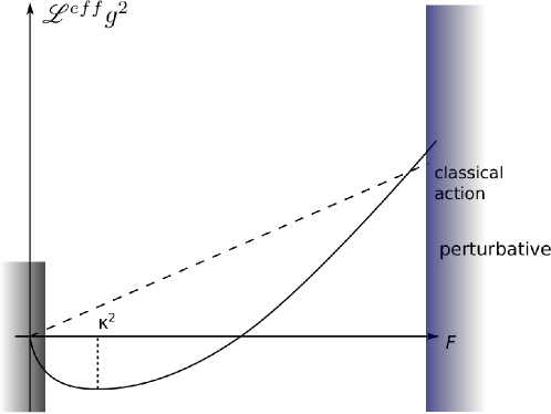
After this prelude we will return to the role of the energy-momentum tensor in Yang-Mills theory. Rather than attempt the difficult task of computing ℒ e f f superscript ℒ 𝑒 𝑓 𝑓 \mathscr{L}^{eff} [DR83 ] , we will instead make an ansatz. Our ansatz will be motivated by the requirements that ℒ e f f ( x ) superscript ℒ 𝑒 𝑓 𝑓 𝑥 \mathscr{L}^{eff}(x) F 2 := F μ ν a F a μ ν assign superscript 𝐹 2 subscript superscript 𝐹 𝑎 𝜇 𝜈 superscript 𝐹 𝑎 𝜇 𝜈 F^{2}:=F^{a}_{\mu\nu}F^{a\mu\nu} [PT78 ] .
So we require
Θ μ ν superscript Θ 𝜇 𝜈 \displaystyle\Theta^{\mu\nu} = 2 ℒ ( F 2 ) ∂ η μ ν − η μ ν ℒ ( F 2 ) absent 2 ℒ superscript 𝐹 2 subscript 𝜂 𝜇 𝜈 superscript 𝜂 𝜇 𝜈 ℒ superscript 𝐹 2 \displaystyle=2\frac{\mathscr{L}(F^{2})}{\partial\eta_{\mu\nu}}-\eta^{\mu\nu}\mathscr{L}(F^{2})
Θ μ μ superscript subscript Θ 𝜇 𝜇 \displaystyle\Theta_{\mu}^{\mu} = β ( g ¯ ( t ) ) 2 g ¯ 3 ( t ) F μ ν a F a μ ν , absent 𝛽 ¯ 𝑔 𝑡 2 superscript ¯ 𝑔 3 𝑡 subscript superscript 𝐹 𝑎 𝜇 𝜈 superscript 𝐹 𝑎 𝜇 𝜈 \displaystyle=\frac{\beta(\bar{g}(t))}{2\bar{g}^{3}(t)}F^{a}_{\mu\nu}F^{a\mu\nu}\ ,
so that Θ μ μ superscript subscript Θ 𝜇 𝜇 \Theta_{\mu}^{\mu}
ℒ e f f := − 1 4 1 g ¯ 2 ( t ) F 2 , t := 1 4 ln F 2 μ 2 . formulae-sequence assign superscript ℒ 𝑒 𝑓 𝑓 1 4 1 superscript ¯ 𝑔 2 𝑡 superscript 𝐹 2 assign 𝑡 1 4 superscript 𝐹 2 superscript 𝜇 2 \mathscr{L}^{eff}:=-\frac{1}{4}\frac{1}{\bar{g}^{2}(t)}F^{2}\ ,\quad t:=\frac{1}{4}\ln\frac{F^{2}}{\mu^{2}}\quad. (30)
So we have to calculate
Θ μ ν subscript Θ 𝜇 𝜈 \displaystyle\Theta_{\mu\nu} = 2 ∂ ℒ e f f ∂ η μ ν − η μ ν ℒ e f f absent 2 superscript ℒ 𝑒 𝑓 𝑓 superscript 𝜂 𝜇 𝜈 subscript 𝜂 𝜇 𝜈 superscript ℒ 𝑒 𝑓 𝑓 \displaystyle=2\frac{\partial\mathscr{L}^{eff}}{\partial\eta^{\mu\nu}}-\eta_{\mu\nu}\mathscr{L}^{eff}
= ( 2 1 g ¯ 2 ( t ) ∂ ∂ η μ ν ( − 1 4 F 2 ) − η μ ν ℒ ) − 2 4 ( ∂ ∂ η μ ν 1 g ¯ 2 ( t ) ) F 2 absent 2 1 superscript ¯ 𝑔 2 𝑡 superscript 𝜂 𝜇 𝜈 1 4 superscript 𝐹 2 subscript 𝜂 𝜇 𝜈 ℒ 2 4 superscript 𝜂 𝜇 𝜈 1 superscript ¯ 𝑔 2 𝑡 superscript 𝐹 2 \displaystyle=\left(2\frac{1}{\bar{g}^{2}(t)}\frac{\partial}{\partial\eta^{\mu\nu}}\left(-\frac{1}{4}F^{2}\right)-\eta_{\mu\nu}\mathscr{L}\right)-\frac{2}{4}\left(\frac{\partial}{\partial\eta^{\mu\nu}}\frac{1}{\bar{g}^{2}(t)}\right)F^{2}
= 1 g ¯ 2 ( t ) [ 1 4 η μ ν F 2 − F μ α F ν α ] − 1 2 ( ∂ t ∂ η μ ν d d t 1 g ¯ 2 ( t ) ) F 2 absent 1 superscript ¯ 𝑔 2 𝑡 delimited-[] 1 4 subscript 𝜂 𝜇 𝜈 superscript 𝐹 2 superscript subscript 𝐹 𝜇 𝛼 subscript 𝐹 𝜈 𝛼 1 2 𝑡 superscript 𝜂 𝜇 𝜈 𝑑 𝑑 𝑡 1 superscript ¯ 𝑔 2 𝑡 superscript 𝐹 2 \displaystyle=\frac{1}{\bar{g}^{2}(t)}\left[\frac{1}{4}\eta_{\mu\nu}F^{2}-F_{\mu}^{\alpha}F_{\nu\alpha}\right]-\frac{1}{2}\left(\frac{\partial t}{\partial\eta^{\mu\nu}}\frac{d}{dt}\frac{1}{\bar{g}^{2}(t)}\right)F^{2}
= 1 g ¯ 2 ( t ) [ F μ α F α ν + 1 4 η μ ν F 2 ] + 1 4 ( d d t 1 g ¯ 2 ( t ) ) F μ β a F ν a β . absent 1 superscript ¯ 𝑔 2 𝑡 delimited-[] superscript subscript 𝐹 𝜇 𝛼 subscript 𝐹 𝛼 𝜈 1 4 subscript 𝜂 𝜇 𝜈 superscript 𝐹 2 1 4 𝑑 𝑑 𝑡 1 superscript ¯ 𝑔 2 𝑡 subscript superscript 𝐹 𝑎 𝜇 𝛽 subscript superscript 𝐹 𝑎 𝛽 𝜈 \displaystyle=\frac{1}{\bar{g}^{2}(t)}\left[F_{\mu}^{\alpha}F_{\alpha\nu}+\frac{1}{4}\eta_{\mu\nu}F^{2}\right]+\frac{1}{4}\left(\frac{d}{dt}\frac{1}{\bar{g}^{2}(t)}\right)F^{a}_{\mu\beta}F^{a\beta}_{\nu}\ .
The last term on the right-hand side uses the result
d d t 1 g ¯ 2 ( t ) = − 2 g ¯ 3 ( t ) d g ¯ d t ( t ) = − 2 β ( g ¯ ( t ) ) g ¯ 3 ( t ) , 𝑑 𝑑 𝑡 1 superscript ¯ 𝑔 2 𝑡 2 superscript ¯ 𝑔 3 𝑡 𝑑 ¯ 𝑔 𝑑 𝑡 𝑡 2 𝛽 ¯ 𝑔 𝑡 superscript ¯ 𝑔 3 𝑡 \frac{d}{dt}\frac{1}{\bar{g}^{2}(t)}=-\frac{2}{\bar{g}^{3}(t)}\frac{d\bar{g}}{dt}(t)=-2\frac{\beta(\bar{g}(t))}{\bar{g}^{3}(t)}\quad, (31)
where we employed
t = ∫ g g ¯ ( t ) d g ′ β ( g ′ ) , 𝑡 superscript subscript 𝑔 ¯ 𝑔 𝑡 𝑑 superscript 𝑔 ′ 𝛽 superscript 𝑔 ′ t=\int_{g}^{\bar{g}(t)}\frac{dg^{\prime}}{\beta(g^{\prime})}\quad, (32)
which, when taken the derivative d d t 𝑑 𝑑 𝑡 \tfrac{d}{dt}
1 = 1 β ( g ¯ ( t ) ) d d t g ¯ ( t ) , i.e., d d t g ¯ ( t ) = β ( g ¯ ( t ) ) . formulae-sequence 1 1 𝛽 ¯ 𝑔 𝑡 𝑑 𝑑 𝑡 ¯ 𝑔 𝑡 i.e., 𝑑 𝑑 𝑡 ¯ 𝑔 𝑡 𝛽 ¯ 𝑔 𝑡 1=\frac{1}{\beta(\bar{g}(t))}\frac{d}{dt}\bar{g}(t),\text{ i.e., }\frac{d}{dt}\bar{g}(t)=\beta(\bar{g}(t))\quad. (33)
So we proved the relation
Θ μ ν subscript Θ 𝜇 𝜈 \displaystyle\Theta_{\mu\nu} = 1 g ¯ 2 ( t ) [ F μ α F α ν + 1 4 η μ ν F 2 ] − β ( g ¯ ( t ) ) 2 g ¯ 3 ( t ) F μ β a F ν a β , absent 1 superscript ¯ 𝑔 2 𝑡 delimited-[] superscript subscript 𝐹 𝜇 𝛼 subscript 𝐹 𝛼 𝜈 1 4 subscript 𝜂 𝜇 𝜈 superscript 𝐹 2 𝛽 ¯ 𝑔 𝑡 2 superscript ¯ 𝑔 3 𝑡 subscript superscript 𝐹 𝑎 𝜇 𝛽 subscript superscript 𝐹 𝑎 𝛽 𝜈 \displaystyle=\frac{1}{\bar{g}^{2}(t)}\left[F_{\mu}^{\alpha}F_{\alpha\nu}+\frac{1}{4}\eta_{\mu\nu}F^{2}\right]-\frac{\beta(\bar{g}(t))}{2\bar{g}^{3}(t)}F^{a}_{\mu\beta}F^{a\beta}_{\nu}\ , and from here the trace
Θ μ μ superscript subscript Θ 𝜇 𝜇 \displaystyle\Theta_{\mu}^{\mu} = β ( g ¯ ( t ) ) 2 g ¯ 3 ( t ) F μ β a F a μ β , t = 1 4 ln F 2 μ 4 . □ \displaystyle=\frac{\beta(\bar{g}(t))}{2\bar{g}^{3}(t)}F^{a}_{\mu\beta}F^{a\mu\beta}\ ,\quad t=\frac{1}{4}\ln\frac{F^{2}}{\mu^{4}}\quad.\quad\square
We also can verify that our ansatz ℒ e f f = − 1 4 F 2 g ¯ 2 ( t ) , t = 1 4 ln F 2 μ 4 formulae-sequence superscript ℒ 𝑒 𝑓 𝑓 1 4 superscript 𝐹 2 superscript ¯ 𝑔 2 𝑡 𝑡 1 4 superscript 𝐹 2 superscript 𝜇 4 \mathscr{L}^{eff}=-\frac{1}{4}\frac{F^{2}}{\bar{g}^{2}(t)},\ t=\frac{1}{4}\ln\frac{F^{2}}{\mu^{4}}
[ μ ∂ ∂ μ + β ( g ) ∂ ∂ g ] ( − 1 4 F 2 ) 1 g ¯ 2 ( t ) = 0 . delimited-[] 𝜇 𝜇 𝛽 𝑔 𝑔 1 4 superscript 𝐹 2 1 superscript ¯ 𝑔 2 𝑡 0 \left[\mu\frac{\partial}{\partial\mu}+\beta(g)\frac{\partial}{\partial g}\right]\left(-\frac{1}{4}F^{2}\right)\frac{1}{\bar{g}^{2}(t)}=0\quad. (34)
Proof:
μ ∂ ∂ μ 1 g ¯ 2 ( t ) 𝜇 𝜇 1 superscript ¯ 𝑔 2 𝑡 \displaystyle\mu\frac{\partial}{\partial\mu}\frac{1}{\bar{g}^{2}(t)} = μ ∂ t ∂ μ d d t 1 g ¯ 2 ( t ) = μ 1 4 ∂ ∂ μ ( ln F 2 − 4 ln μ ) ( − 2 ) β ( g ¯ ( t ) ) g ¯ 3 ( t ) absent 𝜇 𝑡 𝜇 𝑑 𝑑 𝑡 1 superscript ¯ 𝑔 2 𝑡 𝜇 1 4 𝜇 superscript 𝐹 2 4 𝜇 2 𝛽 ¯ 𝑔 𝑡 superscript ¯ 𝑔 3 𝑡 \displaystyle=\mu\frac{\partial t}{\partial\mu}\frac{d}{dt}\frac{1}{\bar{g}^{2}(t)}=\mu\frac{1}{4}\frac{\partial}{\partial\mu}\left(\ln F^{2}-4\ln\mu\right)(-2)\frac{\beta(\bar{g}(t))}{\bar{g}^{3}(t)}
= 2 β ( g ¯ ( t ) ) g ¯ 3 ( t ) . absent 2 𝛽 ¯ 𝑔 𝑡 superscript ¯ 𝑔 3 𝑡 \displaystyle=2\frac{\beta(\bar{g}(t))}{\bar{g}^{3}(t)}\quad.
Taking the derivative ∂ ∂ g 𝑔 \tfrac{\partial}{\partial g} t = ∫ g g ¯ ( t ) d g ′ β ( g ′ ) 𝑡 superscript subscript 𝑔 ¯ 𝑔 𝑡 𝑑 superscript 𝑔 ′ 𝛽 superscript 𝑔 ′ t=\int_{g}^{\bar{g}(t)}\tfrac{dg^{\prime}}{\beta(g^{\prime})}
∂ ∂ g t = 0 = ∂ g ¯ ( t ) ∂ g 1 β ( g ¯ ( t ) ) − 1 β ( g ) or ∂ g ¯ ( t ) ∂ g = β ( g ¯ ( t ) ) β ( g ) 𝑔 𝑡 0 ¯ 𝑔 𝑡 𝑔 1 𝛽 ¯ 𝑔 𝑡 1 𝛽 𝑔 or ¯ 𝑔 𝑡 𝑔 𝛽 ¯ 𝑔 𝑡 𝛽 𝑔 \frac{\partial}{\partial g}t=0=\frac{\partial\bar{g}(t)}{\partial g}\frac{1}{\beta(\bar{g}(t))}-\frac{1}{\beta(g)}\ \text{ or }\ \frac{\partial\bar{g}(t)}{\partial g}=\frac{\beta(\bar{g}(t))}{\beta(g)} (35)
and from here
β ( g ) ∂ ∂ g 1 g ¯ 2 ( t ) = β ( g ) ( − 2 ) g ¯ − 3 ( t ) ∂ g ¯ ( t ) ∂ g = − 2 1 g ¯ 3 ( t ) β ( g ) β ( g ¯ ( t ) ) β ( g ) = − 2 β ( g ¯ ( t ) ) g ¯ 3 ( t ) . 𝛽 𝑔 𝑔 1 superscript ¯ 𝑔 2 𝑡 𝛽 𝑔 2 superscript ¯ 𝑔 3 𝑡 ¯ 𝑔 𝑡 𝑔 2 1 superscript ¯ 𝑔 3 𝑡 𝛽 𝑔 𝛽 ¯ 𝑔 𝑡 𝛽 𝑔 2 𝛽 ¯ 𝑔 𝑡 superscript ¯ 𝑔 3 𝑡 \beta(g)\frac{\partial}{\partial g}\frac{1}{\bar{g}^{2}(t)}=\beta(g)(-2)\bar{g}^{-3}(t)\frac{\partial\bar{g}(t)}{\partial g}=-2\frac{1}{\bar{g}^{3}(t)}\beta(g)\frac{\beta(\bar{g}(t))}{\beta(g)}=-2\frac{\beta(\bar{g}(t))}{\bar{g}^{3}(t)}\ . (36)
So we proved the equation
[ μ ∂ ∂ μ + β ( g ) ∂ ∂ g ] 1 g ¯ 2 ( t ) = 0 . delimited-[] 𝜇 𝜇 𝛽 𝑔 𝑔 1 superscript ¯ 𝑔 2 𝑡 0 \left[\mu\frac{\partial}{\partial\mu}+\beta(g)\frac{\partial}{\partial g}\right]\frac{1}{\bar{g}^{2}(t)}=0\ . (37)
The effective Lagrangian is specified once we know β ( g ) 𝛽 𝑔 \beta(g)
g β ( g ) 𝑔 𝛽 𝑔 \displaystyle g\beta(g) = − 1 2 b 0 g 4 + b 1 g 6 + … absent 1 2 subscript 𝑏 0 superscript 𝑔 4 subscript 𝑏 1 superscript 𝑔 6 … \displaystyle=-\frac{1}{2}b_{0}g^{4}+b_{1}g^{6}+\dots
β ( g ) 𝛽 𝑔 \displaystyle\beta(g) = − 1 2 b 0 g 3 + b 1 g 5 + ⋯ = − 1 2 b 0 g 3 ( 1 − 2 b 1 b 0 g 2 ) + … . absent 1 2 subscript 𝑏 0 superscript 𝑔 3 subscript 𝑏 1 superscript 𝑔 5 ⋯ 1 2 subscript 𝑏 0 superscript 𝑔 3 1 2 subscript 𝑏 1 subscript 𝑏 0 superscript 𝑔 2 … \displaystyle=-\frac{1}{2}b_{0}g^{3}+b_{1}g^{5}+\dots=-\frac{1}{2}b_{0}g^{3}\left(1-2\frac{b_{1}}{b_{0}}g^{2}\right)+\dots\quad.
This we substitute into
t 𝑡 \displaystyle t = ∫ g g ¯ ( t ) d g ′ β ( g ′ ) = − 2 b 0 ∫ g g ¯ ( t ) 1 g ′ 3 ( 1 − 2 b 1 b 0 g ′ 2 + … ) 𝑑 g ′ absent superscript subscript 𝑔 ¯ 𝑔 𝑡 𝑑 superscript 𝑔 ′ 𝛽 superscript 𝑔 ′ 2 subscript 𝑏 0 superscript subscript 𝑔 ¯ 𝑔 𝑡 1 superscript 𝑔 ′ 3
1 2 subscript 𝑏 1 subscript 𝑏 0 superscript 𝑔 ′ 2
… differential-d superscript 𝑔 ′ \displaystyle=\int_{g}^{\bar{g}(t)}\frac{dg^{\prime}}{\beta(g^{\prime})}=-\frac{2}{b_{0}}\int_{g}^{\bar{g}(t)}\frac{1}{g^{\prime 3}(1-2\frac{b_{1}}{b_{0}}g^{\prime 2}+\dots)}dg^{\prime}
= − 2 b 0 ∫ g g ¯ ( t ) ( 1 g ′ 3 + 2 b 1 b 0 1 g ′ + … ) 𝑑 g ′ absent 2 subscript 𝑏 0 superscript subscript 𝑔 ¯ 𝑔 𝑡 1 superscript 𝑔 ′ 3
2 subscript 𝑏 1 subscript 𝑏 0 1 superscript 𝑔 ′ … differential-d superscript 𝑔 ′ \displaystyle=-\frac{2}{b_{0}}\int_{g}^{\bar{g}(t)}\left(\frac{1}{g^{\prime 3}}+2\frac{b_{1}}{b_{0}}\frac{1}{g^{\prime}}+\dots\right)dg^{\prime}
= − 2 b 0 [ − 1 2 g ′ 2 + 2 b 1 b 0 ln g ′ + … ] g g ¯ ( t ) absent 2 subscript 𝑏 0 subscript superscript delimited-[] 1 2 superscript 𝑔 ′ 2
2 subscript 𝑏 1 subscript 𝑏 0 superscript 𝑔 ′ … ¯ 𝑔 𝑡 𝑔 \displaystyle=-\frac{2}{b_{0}}\left[-\frac{1}{2g^{\prime 2}}+2\frac{b_{1}}{b_{0}}\ln g^{\prime}+\dots\right]^{\bar{g}(t)}_{g} to obtain
t 𝑡 \displaystyle t = 1 b 0 1 g ¯ 2 ( t ) − 2 b 0 2 b 1 b 0 ln g ¯ ( t ) + … − 1 b 0 1 g 2 + 2 b 0 2 b 1 b 0 ln g + … ⏟ = const. ⋅ t . absent 1 subscript 𝑏 0 1 superscript ¯ 𝑔 2 𝑡 2 subscript 𝑏 0 2 subscript 𝑏 1 subscript 𝑏 0 ¯ 𝑔 𝑡 … subscript ⏟ 1 subscript 𝑏 0 1 superscript 𝑔 2 2 subscript 𝑏 0 2 subscript 𝑏 1 subscript 𝑏 0 𝑔 … absent ⋅ const. 𝑡 \displaystyle=\frac{1}{b_{0}}\frac{1}{\bar{g}^{2}(t)}-\frac{2}{b_{0}}2\frac{b_{1}}{b_{0}}\ln\bar{g}(t)+\dots\underbrace{-\frac{1}{b_{0}}\frac{1}{g^{2}}+\frac{2}{b_{0}}2\frac{b_{1}}{b_{0}}\ln g+\dots}_{=\text{const.}\cdot t}\quad.
Hence for g ( t ) ≪ 1 much-less-than 𝑔 𝑡 1 g(t)\ll 1
t 𝑡 \displaystyle t = 1 b 0 1 g ¯ ( 1 ) 2 ( t ) absent 1 subscript 𝑏 0 1 subscript superscript ¯ 𝑔 2 1 𝑡 \displaystyle=\frac{1}{b_{0}}\frac{1}{\bar{g}^{2}_{(1)}(t)} : g ¯ ( 1 ) ( t ) : absent subscript ¯ 𝑔 1 𝑡 \displaystyle:\bar{g}_{(1)}(t) = 1 b 0 t absent 1 subscript 𝑏 0 𝑡 \displaystyle=\sqrt{\frac{1}{b_{0}t}}
t 𝑡 \displaystyle t = 1 b 0 1 g ¯ ( 2 ) 2 ( t ) − 2 b 0 2 b 1 b 0 ln 1 b 0 t ⏟ = 1 b 0 2 b 1 b 0 ln t + const. absent 1 subscript 𝑏 0 1 subscript superscript ¯ 𝑔 2 2 𝑡 subscript ⏟ 2 subscript 𝑏 0 2 subscript 𝑏 1 subscript 𝑏 0 1 subscript 𝑏 0 𝑡 absent 1 subscript 𝑏 0 2 subscript 𝑏 1 subscript 𝑏 0 𝑡 const. \displaystyle=\frac{1}{b_{0}}\frac{1}{\bar{g}^{2}_{(2)}(t)}\underbrace{-\frac{2}{b_{0}}2\frac{b_{1}}{b_{0}}\ln\sqrt{\frac{1}{b_{0}t}}}_{=\frac{1}{b_{0}}2\frac{b_{1}}{b_{0}}\ln t+\text{const.}} : 1 g ¯ ( 2 ) 2 ( t ) : absent 1 superscript subscript ¯ 𝑔 2 2 𝑡 \displaystyle:\frac{1}{\bar{g}_{(2)}^{2}(t)} = b 0 t − 2 b 1 b 0 ln t . absent subscript 𝑏 0 𝑡 2 subscript 𝑏 1 subscript 𝑏 0 𝑡 \displaystyle=b_{0}t-2\frac{b_{1}}{b_{0}}\ln t\ .
Consequently for large fields F 2 superscript 𝐹 2 F^{2}
ℒ leading log e f f = − 1 16 b 0 F 2 ln F 2 μ 4 + 𝒪 ( F 2 ln ln F 2 ) . subscript superscript ℒ 𝑒 𝑓 𝑓 leading log 1 16 subscript 𝑏 0 superscript 𝐹 2 superscript 𝐹 2 superscript 𝜇 4 𝒪 superscript 𝐹 2 superscript 𝐹 2 \mathscr{L}^{eff}_{\text{leading log}}=-\frac{1}{16}b_{0}F^{2}\ln\frac{F^{2}}{\mu^{4}}+\mathcal{O}\left(F^{2}\ln\ln F^{2}\right)\quad. (38)
By the way, in QCD we have
β ( g ) 𝛽 𝑔 \displaystyle\beta(g) = μ ∂ g ∂ μ , absent 𝜇 𝑔 𝜇 \displaystyle=\mu\frac{\partial g}{\partial\mu}\quad, where
β ( g ) 𝛽 𝑔 \displaystyle\beta(g) = − g 3 16 π 2 ( 11 3 N − 2 3 N f ) + … absent superscript 𝑔 3 16 superscript 𝜋 2 11 3 𝑁 2 3 subscript 𝑁 𝑓 … \displaystyle=-\frac{g^{3}}{16\pi^{2}}\left(\frac{11}{3}N-\frac{2}{3}N_{f}\right)+\dots
g β ( g ) 𝑔 𝛽 𝑔 \displaystyle g\beta(g) = − 1 2 g 4 1 8 π 2 ( 11 3 N − 2 3 N f ) + 𝒪 ( g 6 ) absent 1 2 superscript 𝑔 4 1 8 superscript 𝜋 2 11 3 𝑁 2 3 subscript 𝑁 𝑓 𝒪 superscript 𝑔 6 \displaystyle=-\frac{1}{2}g^{4}\frac{1}{8\pi^{2}}\left(\frac{11}{3}N-\frac{2}{3}N_{f}\right)+\mathcal{O}(g^{6})
= − 1 2 b 0 g 4 + 𝒪 ( g 6 ) , absent 1 2 subscript 𝑏 0 superscript 𝑔 4 𝒪 superscript 𝑔 6 \displaystyle=-\frac{1}{2}b_{0}g^{4}+\mathcal{O}(g^{6})\quad, so that
b 0 subscript 𝑏 0 \displaystyle b_{0} = 1 8 π 2 ( 11 3 N − 2 3 N f ) . absent 1 8 superscript 𝜋 2 11 3 𝑁 2 3 subscript 𝑁 𝑓 \displaystyle=\frac{1}{8\pi^{2}}\left(\frac{11}{3}N-\frac{2}{3}N_{f}\right)\quad.
Finally, let us write the leading-log effective Lagrangian in a form that will also be useful in QED:
ℒ e f f superscript ℒ 𝑒 𝑓 𝑓 \displaystyle\mathscr{L}^{eff} = − 1 4 1 g ¯ 2 ( t ) F 2 , absent 1 4 1 superscript ¯ 𝑔 2 𝑡 superscript 𝐹 2 \displaystyle=-\frac{1}{4}\frac{1}{\bar{g}^{2}(t)}F^{2}\ ,
t 𝑡 \displaystyle t := 1 4 ln F 2 μ 4 = 1 4 ln 2 ( B 2 − E 2 ) μ 4 assign absent 1 4 superscript 𝐹 2 superscript 𝜇 4 1 4 2 superscript 𝐵 2 superscript 𝐸 2 superscript 𝜇 4 \displaystyle:=\frac{1}{4}\ln\frac{F^{2}}{\mu^{4}}=\frac{1}{4}\ln\frac{2(B^{2}-E^{2})}{\mu^{4}}
F 2 superscript 𝐹 2 \displaystyle F^{2} := F μ ν a F a μ ν = − 2 ( E → a ⋅ E → a − B → a ⋅ B → a ) ≡ − 2 ( E 2 − B 2 ) . assign absent subscript superscript 𝐹 𝑎 𝜇 𝜈 superscript 𝐹 𝑎 𝜇 𝜈 2 ⋅ superscript → 𝐸 𝑎 superscript → 𝐸 𝑎 ⋅ superscript → 𝐵 𝑎 superscript → 𝐵 𝑎 2 superscript 𝐸 2 superscript 𝐵 2 \displaystyle:=F^{a}_{\mu\nu}F^{a\mu\nu}=-2\left(\vec{E}^{a}\cdot\vec{E}^{a}-\vec{B}^{a}\cdot\vec{B}^{a}\right)\equiv-2\left(E^{2}-B^{2}\right)\ .
Then ℒ e f f superscript ℒ 𝑒 𝑓 𝑓 \mathscr{L}^{eff}
ℒ e f f superscript ℒ 𝑒 𝑓 𝑓 \displaystyle\mathscr{L}^{eff} = − 1 4 b 0 t F 2 + ⋯ = − 1 4 b 0 1 4 [ ln F 2 μ 4 ] F 2 + … absent 1 4 subscript 𝑏 0 𝑡 superscript 𝐹 2 ⋯ 1 4 subscript 𝑏 0 1 4 delimited-[] superscript 𝐹 2 superscript 𝜇 4 superscript 𝐹 2 … \displaystyle=-\frac{1}{4}b_{0}tF^{2}+\dots=-\frac{1}{4}b_{0}\frac{1}{4}\left[\ln\frac{F^{2}}{\mu^{4}}\right]F^{2}+\dots
= − 1 16 b 0 F 2 ln F 2 μ 4 + … absent 1 16 subscript 𝑏 0 superscript 𝐹 2 superscript 𝐹 2 superscript 𝜇 4 … \displaystyle=-\frac{1}{16}b_{0}F^{2}\ln\frac{F^{2}}{\mu^{4}}+\dots
ℒ e f f ( 1 ) superscript subscript ℒ 𝑒 𝑓 𝑓 1 \displaystyle\mathscr{L}_{eff}^{(1)} = 1 8 b 0 ( E 2 − B 2 ) ln 2 ( B 2 − E 2 ) μ 4 + … . absent 1 8 subscript 𝑏 0 superscript 𝐸 2 superscript 𝐵 2 2 superscript 𝐵 2 superscript 𝐸 2 superscript 𝜇 4 … \displaystyle=\frac{1}{8}b_{0}(E^{2}-B^{2})\ln\frac{2(B^{2}-E^{2})}{\mu^{4}}+\dots\quad.
When we rescale g 2 superscript 𝑔 2 g^{2}
ℒ e f f = 1 2 ( E → 2 − B → 2 ) + 1 2 ( E → 2 − B → 2 ) g 2 48 π 2 N 11 2 ln g 2 ( B → 2 − E → 2 ) μ 4 + 𝒪 ( F 2 ) . superscript ℒ 𝑒 𝑓 𝑓 1 2 superscript → 𝐸 2 superscript → 𝐵 2 1 2 superscript → 𝐸 2 superscript → 𝐵 2 superscript 𝑔 2 48 superscript 𝜋 2 𝑁 11 2 superscript 𝑔 2 superscript → 𝐵 2 superscript → 𝐸 2 superscript 𝜇 4 𝒪 superscript 𝐹 2 \mathscr{L}^{eff}=\frac{1}{2}\left(\vec{E}^{2}-\vec{B}^{2}\right)+\frac{1}{2}\left(\vec{E}^{2}-\vec{B}^{2}\right)\frac{g^{2}}{48\pi^{2}}N\frac{11}{2}\ln\frac{g^{2}(\vec{B}^{2}-\vec{E}^{2})}{\mu^{4}}+\mathcal{O}(F^{2})\ . (39)
This, by the way, is the same result that one obtains for covariant constant color fields.
Special cases are given by
E → = 0 → : ℒ e f f ( B ) → 𝐸 → 0 : superscript ℒ 𝑒 𝑓 𝑓 𝐵
\displaystyle\vec{E}=\vec{0}\quad:\quad\mathscr{L}^{eff}(B) = − 1 2 B 2 − 1 2 B 2 g 2 48 π 2 N 11 2 ln g 2 B 2 μ 4 absent 1 2 superscript 𝐵 2 1 2 superscript 𝐵 2 superscript 𝑔 2 48 superscript 𝜋 2 𝑁 11 2 superscript 𝑔 2 superscript 𝐵 2 superscript 𝜇 4 \displaystyle=-\frac{1}{2}B^{2}-\frac{1}{2}B^{2}\frac{g^{2}}{48\pi^{2}}N\frac{11}{2}\ln\frac{g^{2}B^{2}}{\mu^{4}}
= − 1 2 B 2 ( 1 + g 2 48 π 2 11 N ln g B μ 2 ) absent 1 2 superscript 𝐵 2 1 superscript 𝑔 2 48 superscript 𝜋 2 11 𝑁 𝑔 𝐵 superscript 𝜇 2 \displaystyle=-\frac{1}{2}B^{2}\left(1+\frac{g^{2}}{48\pi^{2}}11N\ln\frac{gB}{\mu^{2}}\right)
B → 1 i E : ℒ e f f ( E ) → 𝐵 1 𝑖 𝐸 : superscript ℒ 𝑒 𝑓 𝑓 𝐸
\displaystyle B\rightarrow\frac{1}{i}E\quad:\quad\mathscr{L}^{eff}(E) = 1 2 E 2 ( 1 + g 2 48 π 2 11 N ln g ( − i E ) μ 2 ) absent 1 2 superscript 𝐸 2 1 superscript 𝑔 2 48 superscript 𝜋 2 11 𝑁 𝑔 𝑖 𝐸 superscript 𝜇 2 \displaystyle=\frac{1}{2}E^{2}\left(1+\frac{g^{2}}{48\pi^{2}}11N\ln\frac{g(-iE)}{\mu^{2}}\right)
= 1 2 E 2 ( 1 + g 2 48 π 2 11 N ( ln g E μ 2 − i π 2 ) ) . absent 1 2 superscript 𝐸 2 1 superscript 𝑔 2 48 superscript 𝜋 2 11 𝑁 𝑔 𝐸 superscript 𝜇 2 𝑖 𝜋 2 \displaystyle=\frac{1}{2}E^{2}\left(1+\frac{g^{2}}{48\pi^{2}}11N\left(\ln\frac{gE}{\mu^{2}}-\frac{i\pi}{2}\right)\right)\ .
Since V e f f ( B ) = − ℒ e f f ( B ) superscript 𝑉 𝑒 𝑓 𝑓 𝐵 superscript ℒ 𝑒 𝑓 𝑓 𝐵 V^{eff}(B)=-\mathscr{L}^{eff}(B) S U ( N = 3 ) 𝑆 𝑈 𝑁 3 SU(N=3)
V e f f ( B ) = 1 2 B 2 [ 1 + g 2 4 π 2 ( 11 ⋅ 3 − 2 N f ) ln g B μ 2 ] . superscript 𝑉 𝑒 𝑓 𝑓 𝐵 1 2 superscript 𝐵 2 delimited-[] 1 superscript 𝑔 2 4 superscript 𝜋 2 ⋅ 11 3 2 subscript 𝑁 𝑓 𝑔 𝐵 superscript 𝜇 2 V^{eff}(B)=\frac{1}{2}B^{2}\left[1+\frac{g^{2}}{4\pi^{2}}\left(11\cdot 3-2N_{f}\right)\ln\frac{gB}{\mu^{2}}\right]\quad. (40)
Since − 1 4 F 2 = 1 2 ( E 2 − B 2 ) 1 4 superscript 𝐹 2 1 2 superscript 𝐸 2 superscript 𝐵 2 -\tfrac{1}{4}F^{2}=\tfrac{1}{2}(E^{2}-B^{2}) B 2 = 1 2 F 2 superscript 𝐵 2 1 2 superscript 𝐹 2 B^{2}=\tfrac{1}{2}F^{2}
V e f f ( B ) superscript 𝑉 𝑒 𝑓 𝑓 𝐵 \displaystyle V^{eff}(B) = 1 4 F 2 [ 1 + g 2 4 b 0 ln ( g F ) 2 2 μ 4 ] absent 1 4 superscript 𝐹 2 delimited-[] 1 superscript 𝑔 2 4 subscript 𝑏 0 superscript 𝑔 𝐹 2 2 superscript 𝜇 4 \displaystyle=\frac{1}{4}F^{2}\left[1+\frac{g^{2}}{4}b_{0}\ln\frac{(gF)^{2}}{2\mu^{4}}\right]
b 0 subscript 𝑏 0 \displaystyle b_{0} = 1 8 π 2 ( 11 3 ⋅ 3 − 2 3 N f ) , N = 3 . formulae-sequence absent 1 8 superscript 𝜋 2 ⋅ 11 3 3 2 3 subscript 𝑁 𝑓 𝑁 3 \displaystyle=\frac{1}{8\pi^{2}}\left(\frac{11}{3}\cdot 3-\frac{2}{3}N_{f}\right)\ ,\quad N=3\quad.
To find the minimum we take the derivative ∂ V e f f ( F ) ∂ F 2 superscript 𝑉 𝑒 𝑓 𝑓 𝐹 superscript 𝐹 2 \tfrac{\partial V^{eff}(F)}{\partial F^{2}}
ln e ( g F ) 2 2 μ 4 𝑒 superscript 𝑔 𝐹 2 2 superscript 𝜇 4 \displaystyle\ln\frac{e(gF)^{2}}{2\mu^{4}} = − 4 b 0 g 2 absent 4 subscript 𝑏 0 superscript 𝑔 2 \displaystyle=-\frac{4}{b_{0}g^{2}} or
⟨ 0 | ( g F ) 2 | 0 ⟩ quantum-operator-product 0 superscript 𝑔 𝐹 2 0 \displaystyle\langle 0|(gF)^{2}|0\rangle = 2 μ 4 e e − 4 b 0 g 2 , absent 2 superscript 𝜇 4 𝑒 superscript 𝑒 4 subscript 𝑏 0 superscript 𝑔 2 \displaystyle=\frac{2\mu^{4}}{e}e^{-\frac{4}{b_{0}g^{2}}}\quad, which gives the dimensionless number
⟨ 0 | ( g F ) 2 | 0 ⟩ μ 4 quantum-operator-product 0 superscript 𝑔 𝐹 2 0 superscript 𝜇 4 \displaystyle\frac{\langle 0|(gF)^{2}|0\rangle}{\mu^{4}} = 2 e e − 4 b 0 g 2 ⏟ < 1 = 0.7357 e − 4 b 0 g 2 . absent 2 𝑒 subscript ⏟ superscript 𝑒 4 subscript 𝑏 0 superscript 𝑔 2 absent 1 0.7357 superscript 𝑒 4 subscript 𝑏 0 superscript 𝑔 2 \displaystyle=\frac{2}{e}\underbrace{e^{-\frac{4}{b_{0}g^{2}}}}_{<1}=0.7357e^{-\frac{4}{b_{0}g^{2}}}\quad.
From here we find the expression for V m i n e f f ( F ) subscript superscript 𝑉 𝑒 𝑓 𝑓 𝑚 𝑖 𝑛 𝐹 V^{eff}_{min}(F)
V m i n e f f ( F ) subscript superscript 𝑉 𝑒 𝑓 𝑓 𝑚 𝑖 𝑛 𝐹 \displaystyle V^{eff}_{min}(F) = 1 4 ⟨ F 2 ⟩ [ 1 + g 2 4 b 0 ln ⟨ ( g F ) 2 ⟩ 2 μ 4 ] absent 1 4 delimited-⟨⟩ superscript 𝐹 2 delimited-[] 1 superscript 𝑔 2 4 subscript 𝑏 0 delimited-⟨⟩ superscript 𝑔 𝐹 2 2 superscript 𝜇 4 \displaystyle=\frac{1}{4}\langle F^{2}\rangle\left[1+\frac{g^{2}}{4}b_{0}\ln\frac{\langle(gF)^{2}\rangle}{2\mu^{4}}\right]
= 1 4 ⟨ F 2 ⟩ [ 1 + g 2 4 b 0 ( ln 1 e + ln e − 4 b 0 g 2 ) ] absent 1 4 delimited-⟨⟩ superscript 𝐹 2 delimited-[] 1 superscript 𝑔 2 4 subscript 𝑏 0 1 𝑒 superscript 𝑒 4 subscript 𝑏 0 superscript 𝑔 2 \displaystyle=\frac{1}{4}\langle F^{2}\rangle\left[1+\frac{g^{2}}{4}b_{0}\left(\ln\frac{1}{e}+\ln e^{-\frac{4}{b_{0}g^{2}}}\right)\right]
= − b 0 16 ⟨ 0 | ( g F ) 2 | 0 ⟩ ( = 0.7124 ⋅ 10 − 2 ⟨ 0 | ( g F ) 2 | 0 ⟩ for 3 massless flavours ) absent annotated subscript 𝑏 0 16 quantum-operator-product 0 superscript 𝑔 𝐹 2 0 absent ⋅ 0.7124 superscript 10 2 quantum-operator-product 0 superscript 𝑔 𝐹 2 0 for 3 massless flavours \displaystyle=-\frac{b_{0}}{16}\langle 0|(gF)^{2}|0\rangle\quad\left(=0.7124\cdot 10^{-2}\langle 0|(gF)^{2}|0\rangle\text{ for 3 massless flavours}\right)
= − 1 128 π 2 ( 11 − 2 3 N f ) ⟨ 0 | ( g F ) 2 | 0 ⟩ absent 1 128 superscript 𝜋 2 11 2 3 subscript 𝑁 𝑓 quantum-operator-product 0 superscript 𝑔 𝐹 2 0 \displaystyle=-\frac{1}{128\pi^{2}}\left(11-\frac{2}{3}N_{f}\right)\langle 0|(gF)^{2}|0\rangle
= g 2 = 4 π α − 1 128 π 2 ( 11 3 N − 2 3 N f ) ⟨ 0 | 4 π α F 2 | 0 ⟩ superscript 𝑔 2 4 𝜋 𝛼 1 128 superscript 𝜋 2 11 3 𝑁 2 3 subscript 𝑁 𝑓 quantum-operator-product 0 4 𝜋 𝛼 superscript 𝐹 2 0 \displaystyle\underset{g^{2}=4\pi\alpha}{=}-\frac{1}{128\pi^{2}}\left(\frac{11}{3}N-\frac{2}{3}N_{f}\right)\langle 0|4\pi\alpha F^{2}|0\rangle
= − 1 32 ( 11 3 N − 2 3 N f ) ⟨ 0 | α π F μ ν a F a μ ν | 0 ⟩ + 𝒪 ( α 2 ) . absent 1 32 11 3 𝑁 2 3 subscript 𝑁 𝑓 quantum-operator-product 0 𝛼 𝜋 subscript superscript 𝐹 𝑎 𝜇 𝜈 superscript 𝐹 𝑎 𝜇 𝜈 0 𝒪 superscript 𝛼 2 \displaystyle=-\frac{1}{32}\left(\frac{11}{3}N-\frac{2}{3}N_{f}\right)\langle 0|\frac{\alpha}{\pi}F^{a}_{\mu\nu}F^{a\mu\nu}|0\rangle+\mathcal{O}(\alpha^{2})\quad.
This result is consistent with the trace
⟨ 0 | T μ μ | 0 ⟩ = 1 8 ( 11 3 N − 2 3 N f ) ⟨ 0 | α π F μ ν a F a μ ν | 0 ⟩ . quantum-operator-product 0 superscript subscript 𝑇 𝜇 𝜇 0 1 8 11 3 𝑁 2 3 subscript 𝑁 𝑓 quantum-operator-product 0 𝛼 𝜋 subscript superscript 𝐹 𝑎 𝜇 𝜈 superscript 𝐹 𝑎 𝜇 𝜈 0 \langle 0|T_{\mu}^{\mu}|0\rangle=\frac{1}{8}\left(\frac{11}{3}N-\frac{2}{3}N_{f}\right)\langle 0|\frac{\alpha}{\pi}F^{a}_{\mu\nu}F^{a\mu\nu}|0\rangle\ . (41)
From Lorentz invariance T μ ν ( x ) = const. ⋅ g μ ν subscript 𝑇 𝜇 𝜈 𝑥 ⋅ const. subscript 𝑔 𝜇 𝜈 T_{\mu\nu}(x)=\text{const.}\cdot g_{\mu\nu} T 00 = ϵ subscript 𝑇 00 italic-ϵ T_{00}=\epsilon T μ ν = ϵ g μ ν subscript 𝑇 𝜇 𝜈 italic-ϵ subscript 𝑔 𝜇 𝜈 T_{\mu\nu}=\epsilon g_{\mu\nu} T μ μ = 4 ϵ superscript subscript 𝑇 𝜇 𝜇 4 italic-ϵ T_{\mu}^{\mu}=4\epsilon
ϵ = − 1 32 ( 11 3 N − 2 3 N f ) ⟨ 0 | α π F μ ν a F a μ ν | 0 ⟩ + 𝒪 ( α 2 ) . italic-ϵ 1 32 11 3 𝑁 2 3 subscript 𝑁 𝑓 quantum-operator-product 0 𝛼 𝜋 subscript superscript 𝐹 𝑎 𝜇 𝜈 superscript 𝐹 𝑎 𝜇 𝜈 0 𝒪 superscript 𝛼 2 \epsilon=-\frac{1}{32}\left(\frac{11}{3}N-\frac{2}{3}N_{f}\right)\langle 0|\frac{\alpha}{\pi}F^{a}_{\mu\nu}F^{a\mu\nu}|0\rangle+\mathcal{O}(\alpha^{2})\ . (42)
For N = 3 , N f = 3 formulae-sequence 𝑁 3 subscript 𝑁 𝑓 3 N=3,N_{f}=3 ( 11 3 N − 2 3 N f ) = 9 11 3 𝑁 2 3 subscript 𝑁 𝑓 9 (\tfrac{11}{3}N-\tfrac{2}{3}N_{f})=9
0.5 The Effective Lagrangian in QED
We want to investigate the modification of Coulomb’s law for long and short distances. First, we will ask for the effective Lagrangian
for weak, but otherwise arbitrary, fields.
In the weak-field limit, e 2 F μ ν F μ ν / m 4 superscript 𝑒 2 subscript 𝐹 𝜇 𝜈 superscript 𝐹 𝜇 𝜈 superscript 𝑚 4 e^{2}F_{\mu\nu}F^{\mu\nu}/m^{4} α 𝛼 \alpha
W w f ( 1 ) [ A ] = ∫ ℒ w f ( 1 ) d 4 x = 1 2 ∫ A μ ( x ) Π μ ν ( x , y ) A ν ( y ) d 4 x d 4 y superscript subscript 𝑊 𝑤 𝑓 1 delimited-[] 𝐴 subscript superscript ℒ 1 𝑤 𝑓 superscript 𝑑 4 𝑥 1 2 superscript 𝐴 𝜇 𝑥 subscript Π 𝜇 𝜈 𝑥 𝑦 superscript 𝐴 𝜈 𝑦 superscript 𝑑 4 𝑥 superscript 𝑑 4 𝑦 W_{wf}^{(1)}[A]=\int\mathscr{L}^{(1)}_{wf}d^{4}x=\frac{1}{2}\int A^{\mu}(x)\Pi_{\mu\nu}(x,y)A^{\nu}(y)d^{4}xd^{4}y (43)
for the weak-field limit of the one-loop effective action, where Π μ ν subscript Π 𝜇 𝜈 \Pi_{\mu\nu} e 2 superscript 𝑒 2 e^{2}
In momentum space it is given by
Π μ ν ( k ) subscript Π 𝜇 𝜈 𝑘 \displaystyle\Pi_{\mu\nu}(k) = ( g μ ν k 2 − k μ k ν ) Π ( k 2 ) , absent subscript 𝑔 𝜇 𝜈 superscript 𝑘 2 subscript 𝑘 𝜇 subscript 𝑘 𝜈 Π superscript 𝑘 2 \displaystyle=\left(g_{\mu\nu}k^{2}-k_{\mu}k_{\nu}\right)\Pi(k^{2})\ ,
Π ( k 2 ) Π superscript 𝑘 2 \displaystyle\Pi(k^{2}) = − α 3 π k 2 ∫ 4 m 2 ∞ 1 t ρ ( t ) 1 k 2 + t − i ϵ 𝑑 t , absent 𝛼 3 𝜋 superscript 𝑘 2 superscript subscript 4 superscript 𝑚 2 1 𝑡 𝜌 𝑡 1 superscript 𝑘 2 𝑡 𝑖 italic-ϵ differential-d 𝑡 \displaystyle=-\frac{\alpha}{3\pi}k^{2}\int_{4m^{2}}^{\infty}\frac{1}{t}\rho(t)\frac{1}{k^{2}+t-i\epsilon}dt\ ,
ρ ( t ) 𝜌 𝑡 \displaystyle\rho(t) = ( 1 + 2 m 2 t ) ( 1 − 4 m 2 t ) 1 2 . absent 1 2 superscript 𝑚 2 𝑡 superscript 1 4 superscript 𝑚 2 𝑡 1 2 \displaystyle=\left(1+\frac{2m^{2}}{t}\right)\left(1-\frac{4m^{2}}{t}\right)^{\frac{1}{2}}\quad.
As a consequence of the particular tensor structure of Π μ ν ( k ) subscript Π 𝜇 𝜈 𝑘 \Pi_{\mu\nu}(k) W w f ( 1 ) superscript subscript 𝑊 𝑤 𝑓 1 W_{wf}^{(1)} F μ ν subscript 𝐹 𝜇 𝜈 F_{\mu\nu}
Adding the classical Maxwellian term, we obtain for the real field effective Lagrangian
ℒ w f e f f = − 1 4 F μ ν ( x ) [ 1 + α 3 π □ ∫ 4 m 2 ∞ 1 t ρ ( t ) t − □ 𝑑 t ] F μ ν ( x ) subscript superscript ℒ 𝑒 𝑓 𝑓 𝑤 𝑓 1 4 subscript 𝐹 𝜇 𝜈 𝑥 delimited-[] 1 𝛼 3 𝜋 □ superscript subscript 4 superscript 𝑚 2 1 𝑡 𝜌 𝑡 𝑡 □ differential-d 𝑡 superscript 𝐹 𝜇 𝜈 𝑥 \mathscr{L}^{eff}_{wf}=-\frac{1}{4}F_{\mu\nu}(x)\left[1+\frac{\alpha}{3\pi}\square\int_{4m^{2}}^{\infty}\frac{1}{t}\frac{\rho(t)}{t-\square}dt\right]F^{\mu\nu}(x) (44)
where, as usual, □ = − ∂ t 2 + ∇ → 2 □ superscript subscript 𝑡 2 superscript → ∇ 2 \square=-\partial_{t}^{2}+\vec{\nabla}^{2}
The equations of motion resulting from this effective Lagrangian for the weak-field case are linear, because ℒ w f e f f subscript superscript ℒ 𝑒 𝑓 𝑓 𝑤 𝑓 \mathscr{L}^{eff}_{wf} ℒ w f e f f subscript superscript ℒ 𝑒 𝑓 𝑓 𝑤 𝑓 \mathscr{L}^{eff}_{wf}
δ δ A 0 ( x → ) ∫ d 3 x ′ [ 1 2 ∇ → A 0 ⋅ ( 1 + α 3 π ∇ → 2 ∫ 4 m 2 ∞ 1 t ρ ( t ) t − ∇ → 2 𝑑 t ) ∇ → A 0 − A 0 J 0 ] = 0 . 𝛿 𝛿 superscript 𝐴 0 → 𝑥 superscript 𝑑 3 superscript 𝑥 ′ delimited-[] ⋅ 1 2 → ∇ superscript 𝐴 0 1 𝛼 3 𝜋 superscript → ∇ 2 superscript subscript 4 superscript 𝑚 2 1 𝑡 𝜌 𝑡 𝑡 superscript → ∇ 2 differential-d 𝑡 → ∇ superscript 𝐴 0 superscript 𝐴 0 subscript 𝐽 0 0 \frac{\delta}{\delta A^{0}(\vec{x})}\int d^{3}x^{\prime}\left[\frac{1}{2}\vec{\nabla}A^{0}\cdot\left(1+\frac{\alpha}{3\pi}\vec{\nabla}^{2}\int_{4m^{2}}^{\infty}\frac{1}{t}\frac{\rho(t)}{t-\vec{\nabla}^{2}}dt\right)\vec{\nabla}A^{0}-A^{0}J_{0}\right]=0\ . (45)
For J 0 ( x → ) subscript 𝐽 0 → 𝑥 J_{0}(\vec{x}) r 𝑟 r
J 0 ( x → ) = Q [ δ ( x → − x → 1 ) − δ ( x → − x → 2 ) ] , | x → 1 − x → 2 | = r . formulae-sequence subscript 𝐽 0 → 𝑥 𝑄 delimited-[] 𝛿 → 𝑥 subscript → 𝑥 1 𝛿 → 𝑥 subscript → 𝑥 2 subscript → 𝑥 1 subscript → 𝑥 2 𝑟 J_{0}(\vec{x})=Q\left[\delta\left(\vec{x}-\vec{x}_{1}\right)-\delta\left(\vec{x}-\vec{x}_{2}\right)\right]\ ,\quad|\vec{x}_{1}-\vec{x}_{2}|=r\ . (46)
The variation then gives the equation of motion
D ∇ → 2 A 0 ( x → ) 𝐷 superscript → ∇ 2 superscript 𝐴 0 → 𝑥 \displaystyle D\vec{\nabla}^{2}A^{0}(\vec{x}) = − J 0 ( x → ) , absent subscript 𝐽 0 → 𝑥 \displaystyle=-J_{0}(\vec{x})\quad, where
D 𝐷 \displaystyle D := 1 + α 3 π ∇ → 2 ∫ 4 m 2 ∞ 1 t ρ ( t ) t − ∇ → 2 𝑑 t . assign absent 1 𝛼 3 𝜋 superscript → ∇ 2 superscript subscript 4 superscript 𝑚 2 1 𝑡 𝜌 𝑡 𝑡 superscript → ∇ 2 differential-d 𝑡 \displaystyle:=1+\frac{\alpha}{3\pi}\vec{\nabla}^{2}\int_{4m^{2}}^{\infty}\frac{1}{t}\frac{\rho(t)}{t-\vec{\nabla}^{2}}dt\quad.
Making use of the position space representation of the resolvent ( t − ∇ → 2 ) − 1 superscript 𝑡 superscript → ∇ 2 1 (t-\vec{\nabla}^{2})^{-1} V = − ∫ ℒ w f e f f ( A 0 ) d 3 x → 𝑉 superscript subscript ℒ 𝑤 𝑓 𝑒 𝑓 𝑓 superscript 𝐴 0 superscript 𝑑 3 → 𝑥 V=-\int\mathscr{L}_{wf}^{eff}(A^{0})d^{3}\vec{x}
V ( r ) = − Q 2 4 π [ 1 r + α 3 π ∫ 4 m 2 ∞ ρ ( t ) t e − t r r 𝑑 t ] + 𝒪 ( α 2 ) . 𝑉 𝑟 superscript 𝑄 2 4 𝜋 delimited-[] 1 𝑟 𝛼 3 𝜋 superscript subscript 4 superscript 𝑚 2 𝜌 𝑡 𝑡 superscript 𝑒 𝑡 𝑟 𝑟 differential-d 𝑡 𝒪 superscript 𝛼 2 V(r)=-\frac{Q^{2}}{4\pi}\left[\frac{1}{r}+\frac{\alpha}{3\pi}\int_{4m^{2}}^{\infty}\frac{\rho(t)}{t}\frac{e^{-\sqrt{t}r}}{r}dt\right]+\mathcal{O}(\alpha^{2})\ . (47)
The second term in the brackets is the well-known Uehling correction to the classical Coulomb potential. V ( r ) 𝑉 𝑟 V(r) V ( r ) 𝑉 𝑟 V(r)
The quantum mechanical correction to a many-particle static potential,
A 0 ( x → ) superscript 𝐴 0 → 𝑥 \displaystyle A^{0}(\vec{x}) = ∑ i Q i 4 π | x → − x → i | , J 0 ( x → ) = ∑ i Q i δ ( x → − x → i ) formulae-sequence absent subscript 𝑖 subscript 𝑄 𝑖 4 𝜋 → 𝑥 subscript → 𝑥 𝑖 subscript 𝐽 0 → 𝑥 subscript 𝑖 subscript 𝑄 𝑖 𝛿 → 𝑥 subscript → 𝑥 𝑖 \displaystyle=\sum_{i}\frac{Q_{i}}{4\pi|\vec{x}-\vec{x}_{i}|}\ ,\quad J_{0}(\vec{x})=\sum_{i}Q_{i}\delta(\vec{x}-\vec{x}_{i})
V s t a t i c subscript 𝑉 𝑠 𝑡 𝑎 𝑡 𝑖 𝑐 \displaystyle V_{static} = 1 2 ∑ i ≠ j Q i Q j 4 π | x → i − x → j | , r i j = | x → i − x → j | , formulae-sequence absent 1 2 subscript 𝑖 𝑗 subscript 𝑄 𝑖 subscript 𝑄 𝑗 4 𝜋 subscript → 𝑥 𝑖 subscript → 𝑥 𝑗 subscript 𝑟 𝑖 𝑗 subscript → 𝑥 𝑖 subscript → 𝑥 𝑗 \displaystyle=\frac{1}{2}\sum_{i\neq j}\frac{Q_{i}Q_{j}}{4\pi|\vec{x}_{i}-\vec{x}_{j}|}\ ,\quad r_{ij}=|\vec{x}_{i}-\vec{x}_{j}|\ , becomes
V s t a t i c subscript 𝑉 𝑠 𝑡 𝑎 𝑡 𝑖 𝑐 \displaystyle V_{static} = 1 2 ∑ i ≠ j Q i Q j 4 π [ 1 r i j + α 3 π ∫ 4 m 2 ∞ ρ ( t ) t e − t r i j r i j 𝑑 t ] + 𝒪 ( α 2 ) . absent 1 2 subscript 𝑖 𝑗 subscript 𝑄 𝑖 subscript 𝑄 𝑗 4 𝜋 delimited-[] 1 subscript 𝑟 𝑖 𝑗 𝛼 3 𝜋 superscript subscript 4 superscript 𝑚 2 𝜌 𝑡 𝑡 superscript 𝑒 𝑡 subscript 𝑟 𝑖 𝑗 subscript 𝑟 𝑖 𝑗 differential-d 𝑡 𝒪 superscript 𝛼 2 \displaystyle=\frac{1}{2}\sum_{i\neq j}\frac{Q_{i}Q_{j}}{4\pi}\left[\frac{1}{r_{ij}}+\frac{\alpha}{3\pi}\int_{4m^{2}}^{\infty}\frac{\rho(t)}{t}\frac{e^{-\sqrt{t}r_{ij}}}{r_{ij}}dt\right]+\mathcal{O}(\alpha^{2})\ .
Now that we have established the Lagrangian ℒ w f e f f subscript superscript ℒ 𝑒 𝑓 𝑓 𝑤 𝑓 \mathscr{L}^{eff}_{wf}
ℒ e f f = − 1 4 e 2 ( F 2 ) F μ ν F μ ν subscript ℒ 𝑒 𝑓 𝑓 1 4 superscript 𝑒 2 superscript 𝐹 2 subscript 𝐹 𝜇 𝜈 superscript 𝐹 𝜇 𝜈 \mathscr{L}_{eff}=-\frac{1}{4e^{2}(F^{2})}F_{\mu\nu}F^{\mu\nu} (48)
leads to the correct trace anomaly of the energy-momentum tensor (c.f. 0.4
One starts from the free Maxwell Lagrangian
ℒ = − 1 4 F μ ν ( x ) F μ ν ( x ) ℒ 1 4 subscript 𝐹 𝜇 𝜈 𝑥 superscript 𝐹 𝜇 𝜈 𝑥 \mathscr{L}=-\frac{1}{4}F_{\mu\nu}(x)F^{\mu\nu}(x) (49)
and scales the electromagnetic coupling e 𝑒 e
A μ subscript 𝐴 𝜇 \displaystyle A_{\mu} → 1 e A μ , → absent 1 𝑒 subscript 𝐴 𝜇 \displaystyle\rightarrow\frac{1}{e}A_{\mu}\quad, giving
ℒ ℒ \displaystyle\mathscr{L} = − 1 4 e 2 F μ ν F μ ν . absent 1 4 superscript 𝑒 2 subscript 𝐹 𝜇 𝜈 superscript 𝐹 𝜇 𝜈 \displaystyle=-\frac{1}{4e^{2}}F_{\mu\nu}F^{\mu\nu}\ .
Note that in the complete interacting QED Lagrangian this is the only term containing e 𝑒 e ψ ¯ γ ⋅ A ψ ⋅ ¯ 𝜓 𝛾 𝐴 𝜓 \bar{\psi}\gamma\cdot A\psi e ψ ¯ γ ⋅ A ψ ⋅ 𝑒 ¯ 𝜓 𝛾 𝐴 𝜓 e\bar{\psi}\gamma\cdot A\psi
The next step is to renormalization-group improve ℒ ℒ \mathscr{L} e 𝑒 e e ( μ ) 𝑒 𝜇 e(\mu) α 𝛼 \alpha [Ram97 ]
μ ∂ e ∂ μ = β ( e ) = 1 12 π 2 e 3 . 𝜇 𝑒 𝜇 𝛽 𝑒 1 12 superscript 𝜋 2 superscript 𝑒 3 \mu\frac{\partial e}{\partial\mu}=\beta(e)=\frac{1}{12\pi^{2}}e^{3}\ . (50)
This equation is solved by
1 e 2 ( μ ) − 1 e 2 ( μ 0 ) = − 1 6 π 2 ln μ μ 0 , 1 superscript 𝑒 2 𝜇 1 superscript 𝑒 2 subscript 𝜇 0 1 6 superscript 𝜋 2 𝜇 subscript 𝜇 0 \frac{1}{e^{2}(\mu)}-\frac{1}{e^{2}(\mu_{0})}=-\frac{1}{6\pi^{2}}\ln\frac{\mu}{\mu_{0}}\ , (51)
where μ 0 subscript 𝜇 0 \mu_{0}
To prove this let us rewrite the last equation in the form
1 e 2 ( μ ) 1 superscript 𝑒 2 𝜇 \displaystyle\frac{1}{e^{2}(\mu)} = 1 e 2 ( μ 0 ) − 1 6 π 2 ln μ μ 0 absent 1 superscript 𝑒 2 subscript 𝜇 0 1 6 superscript 𝜋 2 𝜇 subscript 𝜇 0 \displaystyle=\frac{1}{e^{2}(\mu_{0})}-\frac{1}{6\pi^{2}}\ln\frac{\mu}{\mu_{0}}
or e ( μ ) or 𝑒 𝜇
\displaystyle\text{or}\qquad e(\mu) = ( 1 e 2 ( μ 0 ) − 1 6 π 2 ln μ μ 0 ) − 1 2 . absent superscript 1 superscript 𝑒 2 subscript 𝜇 0 1 6 superscript 𝜋 2 𝜇 subscript 𝜇 0 1 2 \displaystyle=\left(\frac{1}{e^{2}(\mu_{0})}-\frac{1}{6\pi^{2}}\ln\frac{\mu}{\mu_{0}}\right)^{-\frac{1}{2}}\ . Hence
∂ e ( μ ) ∂ μ 𝑒 𝜇 𝜇 \displaystyle\frac{\partial e(\mu)}{\partial\mu} = − 1 2 ( 1 e 2 ( μ 0 ) − 1 6 π 2 ln μ μ 0 ) − 3 2 ( − 1 6 π 2 ) 1 μ , absent 1 2 superscript 1 superscript 𝑒 2 subscript 𝜇 0 1 6 superscript 𝜋 2 𝜇 subscript 𝜇 0 3 2 1 6 superscript 𝜋 2 1 𝜇 \displaystyle=-\frac{1}{2}\left(\frac{1}{e^{2}(\mu_{0})}-\frac{1}{6\pi^{2}}\ln\frac{\mu}{\mu_{0}}\right)^{-\frac{3}{2}}\left(-\frac{1}{6\pi^{2}}\right)\frac{1}{\mu}\ , which yields
μ ∂ e ( μ ) ∂ μ 𝜇 𝑒 𝜇 𝜇 \displaystyle\mu\frac{\partial e(\mu)}{\partial\mu} = 1 12 e 3 □ absent 1 12 superscript 𝑒 3 □
\displaystyle=\frac{1}{12}e^{3}\qquad\square
Let us rewrite our solution slightly:
1 e 2 ( μ 0 ) ( e 2 ( μ 0 ) e 2 ( μ ) − 1 ) 1 superscript 𝑒 2 subscript 𝜇 0 superscript 𝑒 2 subscript 𝜇 0 superscript 𝑒 2 𝜇 1 \displaystyle\frac{1}{e^{2}(\mu_{0})}\left(\frac{e^{2}(\mu_{0})}{e^{2}(\mu)}-1\right) = − 1 6 π 2 ln μ μ 0 absent 1 6 superscript 𝜋 2 𝜇 subscript 𝜇 0 \displaystyle=-\frac{1}{6\pi^{2}}\ln\frac{\mu}{\mu_{0}}
or e 2 ( μ 0 ) e 2 ( μ ) or superscript 𝑒 2 subscript 𝜇 0 superscript 𝑒 2 𝜇
\displaystyle\text{or}\qquad\frac{e^{2}(\mu_{0})}{e^{2}(\mu)} = 1 − e 2 ( μ 0 ) 6 π 2 ln μ μ 0 . absent 1 superscript 𝑒 2 subscript 𝜇 0 6 superscript 𝜋 2 𝜇 subscript 𝜇 0 \displaystyle=1-\frac{e^{2}(\mu_{0})}{6\pi^{2}}\ln\frac{\mu}{\mu_{0}}\ .
So the scaling equation for e 2 ( μ ) := 4 π α ( μ ) assign superscript 𝑒 2 𝜇 4 𝜋 𝛼 𝜇 e^{2}(\mu):=4\pi\alpha(\mu)
e 2 ( μ ) = e 2 ( μ 0 ) 1 − e 2 ( μ 0 ) 6 π 2 ln μ μ 0 . superscript 𝑒 2 𝜇 superscript 𝑒 2 subscript 𝜇 0 1 superscript 𝑒 2 subscript 𝜇 0 6 superscript 𝜋 2 𝜇 subscript 𝜇 0 e^{2}(\mu)=\frac{e^{2}(\mu_{0})}{1-\frac{e^{2}(\mu_{0})}{6\pi^{2}}\ln\frac{\mu}{\mu_{0}}}\ . (52)
This equation has a singularity which follows from
1 − e 2 ( μ 0 ) 6 π 2 ln μ μ 0 1 superscript 𝑒 2 subscript 𝜇 0 6 superscript 𝜋 2 𝜇 subscript 𝜇 0 \displaystyle 1-\frac{e^{2}(\mu_{0})}{6\pi^{2}}\ln\frac{\mu}{\mu_{0}} = 0 absent 0 \displaystyle=0
or e 2 ( μ 0 ) 6 π 2 ln μ μ 0 or superscript 𝑒 2 subscript 𝜇 0 6 superscript 𝜋 2 𝜇 subscript 𝜇 0
\displaystyle\text{or}\qquad\frac{e^{2}(\mu_{0})}{6\pi^{2}}\ln\frac{\mu}{\mu_{0}} = 1 , absent 1 \displaystyle=1\ ,
which is solved by μ = μ 0 e 6 π 2 e 2 ( μ 0 ) 𝜇 subscript 𝜇 0 superscript 𝑒 6 superscript 𝜋 2 superscript 𝑒 2 subscript 𝜇 0 \mu=\mu_{0}e^{\frac{6\pi^{2}}{e^{2}(\mu_{0})}} e = 0 𝑒 0 e=0
In our application, where the fields are sufficiently strong so that fermionic masses are negligible, the length or mass scale is set by the
magnitude F 2 = F μ ν F μ ν superscript 𝐹 2 subscript 𝐹 𝜇 𝜈 superscript 𝐹 𝜇 𝜈 F^{2}=F_{\mu\nu}F^{\mu\nu} μ 4 superscript 𝜇 4 \mu^{4} F 2 superscript 𝐹 2 F^{2}
e 2 ( F 2 ) = e 2 ( μ 0 ) 1 − e 2 ( μ 0 ) 24 π 2 ln F 2 μ 0 4 , superscript 𝑒 2 superscript 𝐹 2 superscript 𝑒 2 subscript 𝜇 0 1 superscript 𝑒 2 subscript 𝜇 0 24 superscript 𝜋 2 superscript 𝐹 2 superscript subscript 𝜇 0 4 e^{2}(F^{2})=\frac{e^{2}(\mu_{0})}{1-\frac{e^{2}(\mu_{0})}{24\pi^{2}}\ln\frac{F^{2}}{\mu_{0}^{4}}}\ , (53)
with an arbitrary integration constant and arbitrary reference mass μ 0 subscript 𝜇 0 \mu_{0} e 2 superscript 𝑒 2 e^{2} e 2 ( F 2 ) superscript 𝑒 2 superscript 𝐹 2 e^{2}(F^{2})
ℒ e f f subscript ℒ 𝑒 𝑓 𝑓 \displaystyle\mathscr{L}_{eff} = − 1 4 e 2 ( F 2 ) F μ ν F μ ν absent 1 4 superscript 𝑒 2 superscript 𝐹 2 subscript 𝐹 𝜇 𝜈 superscript 𝐹 𝜇 𝜈 \displaystyle=-\frac{1}{4e^{2}(F^{2})}F_{\mu\nu}F^{\mu\nu}
= − 1 4 e 2 ( μ 0 ) F μ ν F μ ν [ 1 − e 2 ( μ 0 ) 24 π 2 ln F 2 μ 0 4 ] . absent 1 4 superscript 𝑒 2 subscript 𝜇 0 subscript 𝐹 𝜇 𝜈 superscript 𝐹 𝜇 𝜈 delimited-[] 1 superscript 𝑒 2 subscript 𝜇 0 24 superscript 𝜋 2 superscript 𝐹 2 superscript subscript 𝜇 0 4 \displaystyle=-\frac{1}{4e^{2}(\mu_{0})}F_{\mu\nu}F^{\mu\nu}\left[1-\frac{e^{2}(\mu_{0})}{24\pi^{2}}\ln\frac{F^{2}}{\mu_{0}^{4}}\right]\ .
The one-loop part is (we scale back e 2 ( μ 0 ) := e 2 assign superscript 𝑒 2 subscript 𝜇 0 superscript 𝑒 2 e^{2}(\mu_{0}):=e^{2}
ℒ ( 1 ) superscript ℒ 1 \displaystyle\mathscr{L}^{(1)} = 1 4 F μ ν F μ ν e 2 24 π 2 ln e 2 F 2 μ 0 4 absent 1 4 subscript 𝐹 𝜇 𝜈 superscript 𝐹 𝜇 𝜈 superscript 𝑒 2 24 superscript 𝜋 2 superscript 𝑒 2 superscript 𝐹 2 superscript subscript 𝜇 0 4 \displaystyle=\frac{1}{4}F_{\mu\nu}F^{\mu\nu}\frac{e^{2}}{24\pi^{2}}\ln\frac{e^{2}F^{2}}{\mu_{0}^{4}}
= F 2 = − 2 ( E → 2 − B → 2 ) 1 2 ( B → 2 − E → 2 ) e 2 24 π 2 ln e 2 ( B → 2 − E → 2 ) μ 0 4 + 𝒪 ( F 2 ) superscript 𝐹 2 2 superscript → 𝐸 2 superscript → 𝐵 2 1 2 superscript → 𝐵 2 superscript → 𝐸 2 superscript 𝑒 2 24 superscript 𝜋 2 superscript 𝑒 2 superscript → 𝐵 2 superscript → 𝐸 2 superscript subscript 𝜇 0 4 𝒪 superscript 𝐹 2 \displaystyle\overset{F^{2}=-2(\vec{E}^{2}-\vec{B}^{2})}{=}\frac{1}{2}\left(\vec{B}^{2}-\vec{E}^{2}\right)\frac{e^{2}}{24\pi^{2}}\ln\frac{e^{2}\left(\vec{B}^{2}-\vec{E}^{2}\right)}{\mu_{0}^{4}}+\mathcal{O}(F^{2})
E → = 0 → : ℒ ( 1 ) ( B ) \displaystyle\vec{E}=\vec{0}:\qquad\mathscr{L}^{(1)}(B) = 1 2 B 2 e 2 24 π 2 ln ( e B ) 2 μ 0 4 = α B 2 6 π ln e B μ 0 2 absent 1 2 superscript 𝐵 2 superscript 𝑒 2 24 superscript 𝜋 2 superscript 𝑒 𝐵 2 superscript subscript 𝜇 0 4 𝛼 superscript 𝐵 2 6 𝜋 𝑒 𝐵 superscript subscript 𝜇 0 2 \displaystyle=\frac{1}{2}B^{2}\frac{e^{2}}{24\pi^{2}}\ln\frac{(eB)^{2}}{\mu_{0}^{4}}=\frac{\alpha B^{2}}{6\pi}\ln\frac{eB}{\mu_{0}^{2}}
B → 1 i E : ℒ ( 1 ) ( E ) \displaystyle B\rightarrow\frac{1}{i}E:\qquad\mathscr{L}^{(1)}(E) = − α E 2 6 π ln e ( − i E ) μ 0 2 absent 𝛼 superscript 𝐸 2 6 𝜋 𝑒 𝑖 𝐸 superscript subscript 𝜇 0 2 \displaystyle=-\frac{\alpha E^{2}}{6\pi}\ln\frac{e(-iE)}{\mu_{0}^{2}}
= − α E 2 6 π ln e E ⋅ e − i π 2 μ 0 2 = − α E 2 6 π [ ln e E μ 0 2 − π 2 i ] absent 𝛼 superscript 𝐸 2 6 𝜋 ⋅ 𝑒 𝐸 superscript 𝑒 𝑖 𝜋 2 superscript subscript 𝜇 0 2 𝛼 superscript 𝐸 2 6 𝜋 delimited-[] 𝑒 𝐸 superscript subscript 𝜇 0 2 𝜋 2 𝑖 \displaystyle=-\frac{\alpha E^{2}}{6\pi}\ln\frac{eE\cdot e^{-i\frac{\pi}{2}}}{\mu_{0}^{2}}=-\frac{\alpha E^{2}}{6\pi}\left[\ln\frac{eE}{\mu_{0}^{2}}-\frac{\pi}{2}i\right]
μ 0 ≡ m : ℒ ( 1 ) ( E ) \displaystyle\mu_{0}\equiv m:\qquad\mathscr{L}^{(1)}(E) = − α E 2 6 π ( ln e E m 2 − π 2 i ) , absent 𝛼 superscript 𝐸 2 6 𝜋 𝑒 𝐸 superscript 𝑚 2 𝜋 2 𝑖 \displaystyle=-\frac{\alpha E^{2}}{6\pi}\left(\ln\frac{eE}{m^{2}}-\frac{\pi}{2}i\right)\quad,
and this is our old formula for ℒ ( 1 ) ( e E m 2 → ∞ ) superscript ℒ 1 → 𝑒 𝐸 superscript 𝑚 2 \mathscr{L}^{(1)}\left(\frac{eE}{m^{2}}\rightarrow\infty\right) ℒ ( 1 ) superscript ℒ 1 \mathscr{L}^{(1)} ℒ ( 1 ) superscript ℒ 1 \mathscr{L}^{(1)} F 2 ln F superscript 𝐹 2 𝐹 F^{2}\ln F
Now that we have established the Lagrangian for strong but otherwise arbitrary fields, we can set up the generalized Maxwell equations and try to solve them
for a given source distribution. In general, they are of the form
δ δ A μ ( x ) ∫ [ ℒ ( 0 ) + ℒ ( 1 ) − J μ A μ ] d 4 x ′ = 0 , 𝛿 𝛿 subscript 𝐴 𝜇 𝑥 delimited-[] superscript ℒ 0 superscript ℒ 1 subscript 𝐽 𝜇 superscript 𝐴 𝜇 superscript 𝑑 4 superscript 𝑥 ′ 0 \frac{\delta}{\delta A_{\mu}(x)}\int\left[\mathscr{L}^{(0)}+\mathscr{L}^{(1)}-J_{\mu}A^{\mu}\right]d^{4}x^{\prime}=0\ , (54)
with ℒ ( 1 ) superscript ℒ 1 \mathscr{L}^{(1)} J μ ( x ) = J 0 ( x → ) δ μ subscript 𝐽 𝜇 𝑥 subscript 𝐽 0 → 𝑥 subscript 𝛿 𝜇 J_{\mu}(x)=J_{0}(\vec{x})\delta_{\mu} E → ( x → ) = − ∇ → A 0 ( x → ) ( A 0 = ϕ ) → 𝐸 → 𝑥 → ∇ superscript 𝐴 0 → 𝑥 superscript 𝐴 0 italic-ϕ \vec{E}(\vec{x})=-\vec{\nabla}A^{0}(\vec{x})\ (A^{0}=\phi)
δ δ A 0 ( x → ) ∫ ( 1 2 | ∇ → A 0 | 2 [ 1 − e 2 12 π 2 ln e | ∇ → A 0 | m 2 ] − J 0 A 0 ) d 3 x → ′ = 0 , 𝛿 𝛿 superscript 𝐴 0 → 𝑥 1 2 superscript → ∇ superscript 𝐴 0 2 delimited-[] 1 superscript 𝑒 2 12 superscript 𝜋 2 𝑒 → ∇ superscript 𝐴 0 superscript 𝑚 2 superscript 𝐽 0 superscript 𝐴 0 superscript 𝑑 3 superscript → 𝑥 ′ 0 \frac{\delta}{\delta A^{0}(\vec{x})}\int\left(\frac{1}{2}|\vec{\nabla}A^{0}|^{2}\left[1-\frac{e^{2}}{12\pi^{2}}\ln\frac{e|\vec{\nabla}A^{0}|}{m^{2}}\right]-J^{0}A^{0}\right)d^{3}\vec{x}^{\prime}=0\ , (55)
which is equivalent to
V s t a t i c = − ext. ϕ ∫ ( 1 2 ( ∇ → ϕ ) 2 [ 1 − α 3 π ln e | ∇ → ϕ | m 2 ] − ϕ J 0 ) d 3 x . subscript 𝑉 𝑠 𝑡 𝑎 𝑡 𝑖 𝑐 subscript ext. italic-ϕ 1 2 superscript → ∇ italic-ϕ 2 delimited-[] 1 𝛼 3 𝜋 𝑒 → ∇ italic-ϕ superscript 𝑚 2 italic-ϕ subscript 𝐽 0 superscript 𝑑 3 𝑥 V_{static}=-\text{ext.}_{\phi}\int\left(\frac{1}{2}(\vec{\nabla}\phi)^{2}\left[1-\frac{\alpha}{3\pi}\ln\frac{e|\vec{\nabla}\phi|}{m^{2}}\right]-\phi J_{0}\right)d^{3}x\ . (56)
The variation of our ϕ italic-ϕ \phi ϕ ≡ A 0 italic-ϕ superscript 𝐴 0 \phi\equiv A^{0}
∂ k ∂ ℒ ∂ ( ∂ k ϕ ) subscript 𝑘 ℒ subscript 𝑘 italic-ϕ \displaystyle\partial_{k}\frac{\partial\mathscr{L}}{\partial(\partial_{k}\phi)} = ∂ ℒ ∂ ϕ , absent ℒ italic-ϕ \displaystyle=\frac{\partial\mathscr{L}}{\partial\phi}\quad, where
ℒ ( ϕ , ∂ i ϕ ) ℒ italic-ϕ subscript 𝑖 italic-ϕ \displaystyle\mathscr{L}(\phi,\partial_{i}\phi) = 1 2 ∂ k ϕ ∂ k ϕ [ 1 − α 6 π ln e 2 ( ∂ k ϕ ) ( ∂ k ϕ ) m 4 ] − ϕ J 0 absent 1 2 subscript 𝑘 italic-ϕ subscript 𝑘 italic-ϕ delimited-[] 1 𝛼 6 𝜋 superscript 𝑒 2 subscript 𝑘 italic-ϕ subscript 𝑘 italic-ϕ superscript 𝑚 4 italic-ϕ subscript 𝐽 0 \displaystyle=\frac{1}{2}\partial_{k}\phi\partial_{k}\phi\left[1-\frac{\alpha}{6\pi}\ln\frac{e^{2}(\partial_{k}\phi)(\partial_{k}\phi)}{m^{4}}\right]-\phi J_{0}
∂ ℒ ∂ ϕ ℒ italic-ϕ \displaystyle\frac{\partial\mathscr{L}}{\partial\phi} = − J 0 absent subscript 𝐽 0 \displaystyle=-J_{0}
∂ ℒ ∂ ( ∂ k ϕ ) ℒ subscript 𝑘 italic-ϕ \displaystyle\frac{\partial\mathscr{L}}{\partial(\partial_{k}\phi)} = ∂ k ϕ ⏟ = − E k [ 1 − α 6 π ln e 2 ( ∂ k ϕ ) ( ∂ k ϕ ) m 4 ] + ( − α 6 π ∂ k ϕ ) . absent subscript ⏟ subscript 𝑘 italic-ϕ absent subscript 𝐸 𝑘 delimited-[] 1 𝛼 6 𝜋 superscript 𝑒 2 subscript 𝑘 italic-ϕ subscript 𝑘 italic-ϕ superscript 𝑚 4 𝛼 6 𝜋 subscript 𝑘 italic-ϕ \displaystyle=\underbrace{\partial_{k}\phi}_{=-E_{k}}\left[1-\frac{\alpha}{6\pi}\ln\frac{e^{2}(\partial_{k}\phi)(\partial_{k}\phi)}{m^{4}}\right]+\left(-\frac{\alpha}{6\pi}\partial_{k}\phi\right)\ . Therefore
∂ k ∂ ℒ ∂ ( ∂ k ϕ ) subscript 𝑘 ℒ subscript 𝑘 italic-ϕ \displaystyle\partial_{k}\frac{\partial\mathscr{L}}{\partial(\partial_{k}\phi)} = ∂ k ( ( − E k ) [ 1 − α 3 π ln e E m 2 ] + ( α 6 π E k ) ) = − J 0 absent subscript 𝑘 subscript 𝐸 𝑘 delimited-[] 1 𝛼 3 𝜋 𝑒 𝐸 superscript 𝑚 2 𝛼 6 𝜋 subscript 𝐸 𝑘 subscript 𝐽 0 \displaystyle=\partial_{k}\left((-E_{k})\left[1-\frac{\alpha}{3\pi}\ln\frac{eE}{m^{2}}\right]+\left(\frac{\alpha}{6\pi}E_{k}\right)\right)=-J_{0}
and thus ∇ → ⋅ [ ( 1 − α 6 π ⏟ ≪ α 3 π ln e E m 2 − α 3 π ln e E m 2 ) E → ] = J 0 . ⋅ → ∇ delimited-[] 1 subscript ⏟ 𝛼 6 𝜋 much-less-than absent 𝛼 3 𝜋 𝑒 𝐸 superscript 𝑚 2 𝛼 3 𝜋 𝑒 𝐸 superscript 𝑚 2 → 𝐸 subscript 𝐽 0 \displaystyle\vec{\nabla}\cdot\left[\left(1-\underbrace{\frac{\alpha}{6\pi}}_{\ll\frac{\alpha}{3\pi}\ln\frac{eE}{m^{2}}}-\frac{\alpha}{3\pi}\ln\frac{eE}{m^{2}}\right)\vec{E}\right]=J_{0}\ .
Alltogether we have
∇ → ⋅ D → ⋅ → ∇ → 𝐷 \displaystyle\vec{\nabla}\cdot\vec{D} = J 0 , absent subscript 𝐽 0 \displaystyle=J_{0}, D → → 𝐷 \displaystyle\vec{D} := ϵ ( E ) E → assign absent italic-ϵ 𝐸 → 𝐸 \displaystyle:=\epsilon(E)\vec{E}
ϵ ( E ) italic-ϵ 𝐸 \displaystyle\epsilon(E) = 1 − α 3 π ln e E m 2 absent 1 𝛼 3 𝜋 𝑒 𝐸 superscript 𝑚 2 \displaystyle=1-\frac{\alpha}{3\pi}\ln\frac{eE}{m^{2}} E → → 𝐸 \displaystyle\vec{E} = − ∇ → ϕ absent → ∇ italic-ϕ \displaystyle=-\vec{\nabla}\phi
These are well-known classical equations from electrostatics of polarizable media. Looking back at the microscopic origin of ϵ ( E ) italic-ϵ 𝐸 \epsilon(E) ϵ ( E ) italic-ϵ 𝐸 \epsilon(E)
To summarize, we can say that in deriving ∇ → ⋅ D → = J 0 ⋅ → ∇ → 𝐷 subscript 𝐽 0 \vec{\nabla}\cdot\vec{D}=J_{0} D → = ϵ ( E ) E → → 𝐷 italic-ϵ 𝐸 → 𝐸 \vec{D}=\epsilon(E)\vec{E} A μ subscript 𝐴 𝜇 A_{\mu}
To gain some insight into the effect produced by the nonlinear medium ϵ ( r ) italic-ϵ 𝑟 \epsilon(r) J 0 subscript 𝐽 0 J_{0} Q 𝑄 Q x → = 0 → → 𝑥 → 0 \vec{x}=\vec{0} − Q 𝑄 -Q
J 0 ( x → ) = Q δ ( x → ) . subscript 𝐽 0 → 𝑥 𝑄 𝛿 → 𝑥 J_{0}(\vec{x})=Q\delta(\vec{x})\ . (57)
Making the spherically symmetric ansatz
D → = Q 4 π r 2 r ^ , E → = Q ( r ) 4 π r 2 r ^ , r = | r → | , formulae-sequence → 𝐷 𝑄 4 𝜋 superscript 𝑟 2 ^ 𝑟 formulae-sequence → 𝐸 𝑄 𝑟 4 𝜋 superscript 𝑟 2 ^ 𝑟 𝑟 → 𝑟 \vec{D}=\frac{Q}{4\pi r^{2}}\hat{r},\quad\vec{E}=\frac{Q(r)}{4\pi r^{2}}\hat{r},\quad r=|\vec{r}|, (58)
the equation
∇ → ⋅ D → = Q δ ( x → ) ⋅ → ∇ → 𝐷 𝑄 𝛿 → 𝑥 \vec{\nabla}\cdot\vec{D}=Q\delta(\vec{x}) (59)
is solved, provided that the function Q ( r ) 𝑄 𝑟 Q(r)
Q = Q ( r ) ϵ ( e Q ( r ) 4 π r 2 ) . 𝑄 𝑄 𝑟 italic-ϵ 𝑒 𝑄 𝑟 4 𝜋 superscript 𝑟 2 Q=Q(r)\epsilon\left(\frac{eQ(r)}{4\pi r^{2}}\right)\ . (60)
The physical interpretation of Q ( r ) 𝑄 𝑟 Q(r) r 𝑟 r x → = 0 → → 𝑥 → 0 \vec{x}=\vec{0} Q ( r ) 𝑄 𝑟 Q(r) Q 𝑄 Q r → ∞ , Q ( r ) → 𝑟 𝑄 𝑟
r\rightarrow\infty,\ Q(r) Q 𝑄 Q
E ( r ) = Q ( r ) 4 π r 2 . 𝐸 𝑟 𝑄 𝑟 4 𝜋 superscript 𝑟 2 E(r)=\frac{Q(r)}{4\pi r^{2}}\ . (61)
One can show that when
e Q ( r ) 4 π ≫ 1 , much-greater-than 𝑒 𝑄 𝑟 4 𝜋 1 \frac{eQ(r)}{4\pi}\gg 1\quad, (62)
the approximation of neglecting the nonlocal one-loop contribution in the effective action becomes self-consistent. To see why this should be so, we note
that because of the leading local but nonlinear correction to ϵ italic-ϵ \epsilon
− α 3 π ln X 1 , X 1 = e Q ( r ) 4 π r 2 m 2 , 𝛼 3 𝜋 subscript 𝑋 1 subscript 𝑋 1
𝑒 𝑄 𝑟 4 𝜋 superscript 𝑟 2 superscript 𝑚 2 -\frac{\alpha}{3\pi}\ln X_{1}\ ,\quad X_{1}=\frac{eQ(r)}{4\pi r^{2}m^{2}}\ , (63)
while for the leading nonlocal correction
− α 3 π ln X 2 , X 2 = ( ∇ → ln A 0 ) 2 m 2 ∼ 1 r 2 m 2 , 𝛼 3 𝜋 subscript 𝑋 2 subscript 𝑋 2
superscript → ∇ superscript 𝐴 0 2 superscript 𝑚 2 similar-to 1 superscript 𝑟 2 superscript 𝑚 2 -\frac{\alpha}{3\pi}\ln X_{2}\ ,\quad X_{2}=\frac{\left(\vec{\nabla}\ln A^{0}\right)^{2}}{m^{2}}\sim\frac{1}{r^{2}m^{2}}\ , (64)
so that e Q ( r ) 4 π ≫ 1 much-greater-than 𝑒 𝑄 𝑟 4 𝜋 1 \tfrac{eQ(r)}{4\pi}\gg 1 X 1 ≫ X 2 much-greater-than subscript 𝑋 1 subscript 𝑋 2 X_{1}\gg X_{2}
0.6 Adler’s Leading-Log Model in QCD
Here, the leading approximation to the effective action is obtained by replacing g 2 superscript 𝑔 2 g^{2}
ℒ = 1 2 g 2 ( E → 2 − B → 2 ) , ℒ 1 2 superscript 𝑔 2 superscript → 𝐸 2 superscript → 𝐵 2 \mathscr{L}=\frac{1}{2g^{2}}\left(\vec{E}^{2}-\vec{B}^{2}\right)\ , (65)
by the running coupling constant
ℒ e f f superscript ℒ 𝑒 𝑓 𝑓 \displaystyle\mathscr{L}^{eff} = 1 2 g r u n n i n g 2 ( E → 2 − B → 2 ) , absent 1 2 subscript superscript 𝑔 2 𝑟 𝑢 𝑛 𝑛 𝑖 𝑛 𝑔 superscript → 𝐸 2 superscript → 𝐵 2 \displaystyle=\frac{1}{2g^{2}_{running}}\left(\vec{E}^{2}-\vec{B}^{2}\right)\ , where
g r u n n i n g 2 ( E → 2 − B 2 → μ 4 ) subscript superscript 𝑔 2 𝑟 𝑢 𝑛 𝑛 𝑖 𝑛 𝑔 superscript → 𝐸 2 → superscript 𝐵 2 superscript 𝜇 4 \displaystyle g^{2}_{running}\left(\frac{\vec{E}^{2}-\vec{B^{2}}}{\mu^{4}}\right) = g 2 ( μ 2 ) 1 + 1 4 b 0 g 2 ( μ 2 ) ln ( E → 2 − B 2 → μ 4 ) , absent superscript 𝑔 2 superscript 𝜇 2 1 1 4 subscript 𝑏 0 superscript 𝑔 2 superscript 𝜇 2 superscript → 𝐸 2 → superscript 𝐵 2 superscript 𝜇 4 \displaystyle=\frac{g^{2}(\mu^{2})}{1+\frac{1}{4}b_{0}g^{2}(\mu^{2})\ln\left(\frac{\vec{E}^{2}-\vec{B^{2}}}{\mu^{4}}\right)}\ , so that
ℒ e f f superscript ℒ 𝑒 𝑓 𝑓 \displaystyle\mathscr{L}^{eff} = 1 2 g 2 ( E → 2 − B → 2 ) [ 1 + 1 4 b 0 g 2 ( μ 2 ) ln ( E → 2 − B 2 → μ 4 ) ] . absent 1 2 superscript 𝑔 2 superscript → 𝐸 2 superscript → 𝐵 2 delimited-[] 1 1 4 subscript 𝑏 0 superscript 𝑔 2 superscript 𝜇 2 superscript → 𝐸 2 → superscript 𝐵 2 superscript 𝜇 4 \displaystyle=\frac{1}{2g^{2}}\left(\vec{E}^{2}-\vec{B}^{2}\right)\left[1+\frac{1}{4}b_{0}g^{2}(\mu^{2})\ln\left(\frac{\vec{E}^{2}-\vec{B^{2}}}{\mu^{4}}\right)\right]\ .
Here μ 𝜇 \mu g 2 = g 2 ( μ 2 ) superscript 𝑔 2 superscript 𝑔 2 superscript 𝜇 2 g^{2}=g^{2}(\mu^{2}) b 0 subscript 𝑏 0 b_{0}
b 0 = 1 8 π 2 11 3 C a d > 0 . subscript 𝑏 0 1 8 superscript 𝜋 2 11 3 subscript 𝐶 𝑎 𝑑 0 b_{0}=\frac{1}{8\pi^{2}}\frac{11}{3}C_{ad}>0\ . (66)
Our formula for ℒ e f f superscript ℒ 𝑒 𝑓 𝑓 \mathscr{L}^{eff} g r u n n i n g 2 subscript superscript 𝑔 2 𝑟 𝑢 𝑛 𝑛 𝑖 𝑛 𝑔 g^{2}_{running}
( E → 2 − B → 2 ) superscript → 𝐸 2 superscript → 𝐵 2 \displaystyle\left(\vec{E}^{2}-\vec{B}^{2}\right) ≫ μ 4 much-greater-than absent superscript 𝜇 4 \displaystyle\gg\mu^{4}
E → , B → → 𝐸 → 𝐵
\displaystyle\vec{E},\vec{B} ≈ 0 → : g 2 small, g 2 < 0 . : absent → 0 superscript 𝑔 2 small, superscript 𝑔 2 0 \displaystyle\approx\vec{0}\ :\ g^{2}\text{ small, }g^{2}<0\ .
The variational equation will be
δ W e f f δ ( E , B ) = 0 , 𝛿 superscript 𝑊 𝑒 𝑓 𝑓 𝛿 𝐸 𝐵 0 \frac{\delta W^{eff}}{\delta(E,B)}=0\quad, (67)
and the static potential follows from
V s t a t i c = − W e x t r e m u m e f f + self energies . subscript 𝑉 𝑠 𝑡 𝑎 𝑡 𝑖 𝑐 subscript superscript 𝑊 𝑒 𝑓 𝑓 𝑒 𝑥 𝑡 𝑟 𝑒 𝑚 𝑢 𝑚 self energies V_{static}=-W^{eff}_{extremum}+\text{self energies}\ . (68)
A reminder:
ℒ ℒ \displaystyle\mathscr{L} = − 1 4 F μ ν F μ ν + j μ A μ absent 1 4 subscript 𝐹 𝜇 𝜈 superscript 𝐹 𝜇 𝜈 subscript 𝑗 𝜇 superscript 𝐴 𝜇 \displaystyle=-\frac{1}{4}F_{\mu\nu}F^{\mu\nu}+j_{\mu}A^{\mu}
j → = 0 → W → 𝑗 → 0 𝑊
\displaystyle\vec{j}=\vec{0}\quad W = ∫ [ 1 2 ( E → 2 − B → 2 ) − ρ φ ] d 3 x , W = action T formulae-sequence absent delimited-[] 1 2 superscript → 𝐸 2 superscript → 𝐵 2 𝜌 𝜑 superscript 𝑑 3 𝑥 𝑊 action 𝑇 \displaystyle=\int\left[\frac{1}{2}\left(\vec{E}^{2}-\vec{B}^{2}\right)-\rho\varphi\right]d^{3}x,\quad W=\frac{\text{action}}{T}
δ W δ B = 0 ⇒ B → = 0 → W formulae-sequence 𝛿 𝑊 𝛿 𝐵 0 ⇒ → 𝐵 → 0 𝑊 \displaystyle\frac{\delta W}{\delta B}=0\Rightarrow\vec{B}=\vec{0}\quad W = ∫ [ 1 2 ( ∇ → φ ) 2 − ρ φ ] d 3 x absent delimited-[] 1 2 superscript → ∇ 𝜑 2 𝜌 𝜑 superscript 𝑑 3 𝑥 \displaystyle=\int\left[\frac{1}{2}(\vec{\nabla}\varphi)^{2}-\rho\varphi\right]d^{3}x
δ W 𝛿 𝑊 \displaystyle\delta W = ∫ [ ∇ → φ ⋅ ∇ → δ φ − ρ δ φ ] d 3 x absent delimited-[] ⋅ → ∇ 𝜑 → ∇ 𝛿 𝜑 𝜌 𝛿 𝜑 superscript 𝑑 3 𝑥 \displaystyle=\int\left[\vec{\nabla}\varphi\cdot\vec{\nabla}\delta\varphi-\rho\delta\varphi\right]d^{3}x
= ∫ ( − ∇ → 2 φ − ρ ) δ φ d 3 x = 0 . absent superscript → ∇ 2 𝜑 𝜌 𝛿 𝜑 superscript 𝑑 3 𝑥 0 \displaystyle=\int\left(-\vec{\nabla}^{2}\varphi-\rho\right)\delta\varphi d^{3}x=0\quad.
Thus φ e x t r . subscript 𝜑 𝑒 𝑥 𝑡 𝑟
\varphi_{extr.} ∇ → 2 φ e x t r . = − ρ superscript → ∇ 2 subscript 𝜑 𝑒 𝑥 𝑡 𝑟
𝜌 \vec{\nabla}^{2}\varphi_{extr.}=-\rho
W e x t r . := W [ φ e x t r . ] assign subscript 𝑊 𝑒 𝑥 𝑡 𝑟
𝑊 delimited-[] subscript 𝜑 𝑒 𝑥 𝑡 𝑟
\displaystyle W_{extr.}:=W[\varphi_{extr.}] = ∫ [ 1 2 ∇ → φ ⋅ ∇ → φ − ρ φ ] d 3 x absent delimited-[] ⋅ 1 2 → ∇ 𝜑 → ∇ 𝜑 𝜌 𝜑 superscript 𝑑 3 𝑥 \displaystyle=\int\left[\frac{1}{2}\vec{\nabla}\varphi\cdot\vec{\nabla}\varphi-\rho\varphi\right]d^{3}x
= ∫ [ − 1 2 φ ∇ → 2 φ − ρ φ ] d 3 x absent delimited-[] 1 2 𝜑 superscript → ∇ 2 𝜑 𝜌 𝜑 superscript 𝑑 3 𝑥 \displaystyle=\int\left[-\frac{1}{2}\varphi\vec{\nabla}^{2}\varphi-\rho\varphi\right]d^{3}x
= ∫ [ − 1 2 φ ( − ρ ) − ρ φ ] d 3 x absent delimited-[] 1 2 𝜑 𝜌 𝜌 𝜑 superscript 𝑑 3 𝑥 \displaystyle=\int\left[-\frac{1}{2}\varphi(-\rho)-\rho\varphi\right]d^{3}x
= − 1 2 ∫ ρ φ d 3 x = − V s t a t i c + self energies . absent 1 2 𝜌 𝜑 superscript 𝑑 3 𝑥 subscript 𝑉 𝑠 𝑡 𝑎 𝑡 𝑖 𝑐 self energies \displaystyle=-\frac{1}{2}\int\rho\varphi d^{3}x=-V_{static}+\text{self energies}.
Before we continue, let us rewrite ℒ e f f superscript ℒ 𝑒 𝑓 𝑓 \mathscr{L}^{eff} F 𝐹 F F 2 superscript 𝐹 2 F^{2} F := E → 2 − B → 2 , E → = − ∇ → φ , B → = ∇ → × A → formulae-sequence assign 𝐹 superscript → 𝐸 2 superscript → 𝐵 2 formulae-sequence → 𝐸 → ∇ 𝜑 → 𝐵 → ∇ → 𝐴 F:=\vec{E}^{2}-\vec{B}^{2},\quad\vec{E}=-\vec{\nabla}\varphi,\quad\vec{B}=\vec{\nabla}\times\vec{A}
ℒ e f f ( F ) superscript ℒ 𝑒 𝑓 𝑓 𝐹 \displaystyle\mathscr{L}^{eff}(F) = 1 8 b 0 F [ 4 g 2 ( μ 2 ) b 0 + ln F μ 4 ] absent 1 8 subscript 𝑏 0 𝐹 delimited-[] 4 superscript 𝑔 2 superscript 𝜇 2 subscript 𝑏 0 𝐹 superscript 𝜇 4 \displaystyle=\frac{1}{8}b_{0}F\left[\frac{4}{g^{2}(\mu^{2})b_{0}}+\ln\frac{F}{\mu^{4}}\right]
= 1 8 b 0 F [ − ln e − 4 g 2 ( μ 2 ) b 0 + ln F μ 4 ] absent 1 8 subscript 𝑏 0 𝐹 delimited-[] superscript 𝑒 4 superscript 𝑔 2 superscript 𝜇 2 subscript 𝑏 0 𝐹 superscript 𝜇 4 \displaystyle=\frac{1}{8}b_{0}F\left[-\ln e^{-\frac{4}{g^{2}(\mu^{2})b_{0}}}+\ln\frac{F}{\mu^{4}}\right]
= 1 8 b 0 F ln F μ 4 e − 4 / g 2 ( μ 2 ) b 0 absent 1 8 subscript 𝑏 0 𝐹 𝐹 superscript 𝜇 4 superscript 𝑒 4 superscript 𝑔 2 superscript 𝜇 2 subscript 𝑏 0 \displaystyle=\frac{1}{8}b_{0}F\ln\frac{F}{\mu^{4}e^{-4/g^{2}(\mu^{2})b_{0}}}
ℒ e f f superscript ℒ 𝑒 𝑓 𝑓 \displaystyle\mathscr{L}^{eff} = 1 8 b 0 ln F e κ 2 , absent 1 8 subscript 𝑏 0 𝐹 𝑒 superscript 𝜅 2 \displaystyle=\frac{1}{8}b_{0}\ln\frac{F}{e\kappa^{2}}\ , where κ 2 superscript 𝜅 2 \kappa^{2}
κ 2 superscript 𝜅 2 \displaystyle\kappa^{2} := μ 4 e e − 4 b 0 g 2 ( μ 2 ) . assign absent superscript 𝜇 4 𝑒 superscript 𝑒 4 subscript 𝑏 0 superscript 𝑔 2 superscript 𝜇 2 \displaystyle:=\frac{\mu^{4}}{e}e^{-\frac{4}{b_{0}g^{2}(\mu^{2})}}\ .
This constant, κ 𝜅 \kappa μ 𝜇 \mu g 2 ( μ 2 ) superscript 𝑔 2 superscript 𝜇 2 g^{2}(\mu^{2}) κ 2 superscript 𝜅 2 \kappa^{2} κ 𝜅 \kappa μ 𝜇 \mu
β ( g ) = μ ∂ g ∂ μ = − 1 2 g 3 b 0 . 𝛽 𝑔 𝜇 𝑔 𝜇 1 2 superscript 𝑔 3 subscript 𝑏 0 \beta(g)=\mu\frac{\partial g}{\partial\mu}=-\frac{1}{2}g^{3}b_{0}\quad. (69)
Then we obtain
d d μ κ 2 𝑑 𝑑 𝜇 superscript 𝜅 2 \displaystyle\frac{d}{d\mu}\kappa^{2} = 1 e [ 4 μ 3 e − 4 b 0 g 2 + μ 4 d d μ ( − 4 b 0 g 2 ) e − 4 b 0 g 2 ] absent 1 𝑒 delimited-[] 4 superscript 𝜇 3 superscript 𝑒 4 subscript 𝑏 0 superscript 𝑔 2 superscript 𝜇 4 𝑑 𝑑 𝜇 4 subscript 𝑏 0 superscript 𝑔 2 superscript 𝑒 4 subscript 𝑏 0 superscript 𝑔 2 \displaystyle=\frac{1}{e}\left[4\mu^{3}e^{-\frac{4}{b_{0}g^{2}}}+\mu^{4}\frac{d}{d\mu}\left(-\frac{4}{b_{0}g^{2}}\right)e^{-\frac{4}{b_{0}g^{2}}}\right]
= 1 e e − 4 b 0 g 2 [ 4 μ 3 − 4 μ 4 b 0 ( − 2 ) g − 3 d g d μ ] absent 1 𝑒 superscript 𝑒 4 subscript 𝑏 0 superscript 𝑔 2 delimited-[] 4 superscript 𝜇 3 4 superscript 𝜇 4 subscript 𝑏 0 2 superscript 𝑔 3 𝑑 𝑔 𝑑 𝜇 \displaystyle=\frac{1}{e}e^{-\frac{4}{b_{0}g^{2}}}\left[4\mu^{3}-\frac{4\mu^{4}}{b_{0}}(-2)g^{-3}\frac{dg}{d\mu}\right]
= 1 e e − 4 b 0 g 2 4 μ 3 [ 1 + 2 b 0 g 3 μ ∂ g ∂ μ ⏟ − b 0 2 g 3 ] = 0 . absent 1 𝑒 superscript 𝑒 4 subscript 𝑏 0 superscript 𝑔 2 4 superscript 𝜇 3 delimited-[] 1 2 subscript 𝑏 0 superscript 𝑔 3 subscript ⏟ 𝜇 𝑔 𝜇 subscript 𝑏 0 2 superscript 𝑔 3 0 \displaystyle=\frac{1}{e}e^{-\frac{4}{b_{0}g^{2}}}4\mu^{3}\left[1+\frac{2}{b_{0}g^{3}}\underbrace{\mu\frac{\partial g}{\partial\mu}}_{-\frac{b_{0}}{2}g^{3}}\right]=0\quad.
The graph of ℒ e f f superscript ℒ 𝑒 𝑓 𝑓 \mathscr{L}^{eff} 1
Figure 1: Schematic graph of ℒ e f f superscript ℒ 𝑒 𝑓 𝑓 \mathscr{L}^{eff}
The minimum of ℒ e f f superscript ℒ 𝑒 𝑓 𝑓 \mathscr{L}^{eff}
( F ln F e κ 2 ) ′ superscript 𝐹 𝐹 𝑒 superscript 𝜅 2 ′ \displaystyle\left(F\ln\frac{F}{e\kappa^{2}}\right)^{\prime} = ( F ln F − F ln e κ 2 ) ′ = ln F + 1 − ln e κ 2 absent superscript 𝐹 𝐹 𝐹 𝑒 superscript 𝜅 2 ′ 𝐹 1 𝑒 superscript 𝜅 2 \displaystyle=\left(F\ln F-F\ln e\kappa^{2}\right)^{\prime}=\ln F+1-\ln e\kappa^{2}
= ln F − ln κ 2 = 0 absent 𝐹 superscript 𝜅 2 0 \displaystyle=\ln F-\ln\kappa^{2}=0
⇒ F m i n ⇒ absent subscript 𝐹 𝑚 𝑖 𝑛 \displaystyle\Rightarrow F_{min} = κ 2 = μ 4 e e − 4 b 0 g 2 ( μ 2 ) , b 0 > 0 . formulae-sequence absent superscript 𝜅 2 superscript 𝜇 4 𝑒 superscript 𝑒 4 subscript 𝑏 0 superscript 𝑔 2 superscript 𝜇 2 subscript 𝑏 0 0 \displaystyle=\kappa^{2}=\frac{\mu^{4}}{e}e^{-\frac{4}{b_{0}g^{2}(\mu^{2})}},\quad b_{0}>0\quad.
The renormalization group argument says that ℒ e f f ( F ) superscript ℒ 𝑒 𝑓 𝑓 𝐹 \mathscr{L}^{eff}(F)
W e f f = ∫ [ ℒ e f f − ρ φ ] d 3 x , superscript 𝑊 𝑒 𝑓 𝑓 delimited-[] superscript ℒ 𝑒 𝑓 𝑓 𝜌 𝜑 superscript 𝑑 3 𝑥 W^{eff}=\int\left[\mathscr{L}^{eff}-\rho\varphi\right]d^{3}x\ , (70)
with
ρ ( x → ) = Q [ δ ( 3 ) ( x → − x → 1 ) − δ ( 3 ) ( x → − x → 2 ) ] . 𝜌 → 𝑥 𝑄 delimited-[] superscript 𝛿 3 → 𝑥 subscript → 𝑥 1 superscript 𝛿 3 → 𝑥 subscript → 𝑥 2 \rho(\vec{x})=Q\left[\delta^{(3)}(\vec{x}-\vec{x}_{1})-\delta^{(3)}(\vec{x}-\vec{x}_{2})\right]\ . (71)
The variational equations come from
W e f f superscript 𝑊 𝑒 𝑓 𝑓 \displaystyle W^{eff} = ∫ [ ℒ e f f ( ∇ → φ , A → ) − ρ φ ] d 3 x absent delimited-[] superscript ℒ 𝑒 𝑓 𝑓 → ∇ 𝜑 → 𝐴 𝜌 𝜑 superscript 𝑑 3 𝑥 \displaystyle=\int\left[\mathscr{L}^{eff}(\vec{\nabla}\varphi,\vec{A})-\rho\varphi\right]d^{3}x
ℒ ≡ ℒ e f f : ∇ → ⋅ ∂ ℒ ∂ ( ∇ → φ ) − ∂ ℒ ∂ φ \displaystyle\mathscr{L}\equiv\mathscr{L}^{eff}:\quad\vec{\nabla}\cdot\frac{\partial\mathscr{L}}{\partial(\vec{\nabla}\varphi)}-\frac{\partial\mathscr{L}}{\partial\varphi} = 0 absent 0 \displaystyle=0 1 2 F = 1 2 ( E → 2 − B → 2 ) 1 2 𝐹 1 2 superscript → 𝐸 2 superscript → 𝐵 2 \displaystyle\frac{1}{2}F=\frac{1}{2}\left(\vec{E}^{2}-\vec{B}^{2}\right) = 1 2 [ ( ∇ → φ ) 2 − ( ∇ → × A → ) 2 ] absent 1 2 delimited-[] superscript → ∇ 𝜑 2 superscript → ∇ → 𝐴 2 \displaystyle=\frac{1}{2}\left[(\vec{\nabla}\varphi)^{2}-\left(\vec{\nabla}\times\vec{A}\right)^{2}\right]
or ∇ → ⋅ ∂ ℒ ∂ 1 2 F ⏟ = : ϵ ∂ 1 2 F ∂ ( ∇ → φ ) ⏟ = − E → + ρ or ⋅ → ∇ subscript ⏟ ℒ 1 2 𝐹 : absent italic-ϵ
subscript ⏟ 1 2 𝐹 → ∇ 𝜑 absent → 𝐸 𝜌
\displaystyle\text{or}\quad\vec{\nabla}\cdot\underbrace{\frac{\partial\mathscr{L}}{\partial\frac{1}{2}F}}_{=:\epsilon}\underbrace{\frac{\partial\frac{1}{2}F}{\partial(\vec{\nabla}\varphi)}}_{=-\vec{E}}+\rho = 0 absent 0 \displaystyle=0 ∂ 1 2 F ∂ ( ∇ → φ ) = ∇ → φ 1 2 𝐹 → ∇ 𝜑 → ∇ 𝜑 \displaystyle\frac{\partial\frac{1}{2}F}{\partial(\vec{\nabla}\varphi)}=\vec{\nabla}\varphi = − E → absent → 𝐸 \displaystyle=-\vec{E}
⟹ ∇ → ⋅ ϵ E → ⟹ absent ⋅ → ∇ italic-ϵ → 𝐸 \displaystyle\Longrightarrow\vec{\nabla}\cdot\epsilon\vec{E} = ρ absent 𝜌 \displaystyle=\rho
δ ℒ ( x ) δ A i ( z ) 𝛿 ℒ 𝑥 𝛿 subscript 𝐴 𝑖 𝑧 \displaystyle\frac{\delta\mathscr{L}(x)}{\delta A_{i}(z)} = ∫ ∂ ℒ ( x ) ∂ B j ( x ) δ B j ( x ) δ A i ( z ) 𝑑 x absent ℒ 𝑥 subscript 𝐵 𝑗 𝑥 𝛿 subscript 𝐵 𝑗 𝑥 𝛿 subscript 𝐴 𝑖 𝑧 differential-d 𝑥 \displaystyle=\int\frac{\partial\mathscr{L}(x)}{\partial B_{j}(x)}\frac{\delta B_{j}(x)}{\delta A_{i}(z)}dx
= ∫ ∂ ℒ ( x ) ∂ 1 2 F ( x ) ∂ 1 2 F ∂ B j ( x ) δ δ A i ( z ) ϵ j m n ∂ m A n ( x ) d x absent ℒ 𝑥 1 2 𝐹 𝑥 1 2 𝐹 subscript 𝐵 𝑗 𝑥 𝛿 𝛿 subscript 𝐴 𝑖 𝑧 subscript italic-ϵ 𝑗 𝑚 𝑛 subscript 𝑚 subscript 𝐴 𝑛 𝑥 𝑑 𝑥 \displaystyle=\int\frac{\partial\mathscr{L}(x)}{\partial\frac{1}{2}F(x)}\frac{\partial\frac{1}{2}F}{\partial B_{j}(x)}\frac{\delta}{\delta A_{i}(z)}\epsilon_{jmn}\partial_{m}A_{n}(x)dx
= ∫ ( − ϵ B j ) ( x ) ϵ j m n δ i n ∂ m δ ( x − z ) d x absent italic-ϵ subscript 𝐵 𝑗 𝑥 subscript italic-ϵ 𝑗 𝑚 𝑛 subscript 𝛿 𝑖 𝑛 subscript 𝑚 𝛿 𝑥 𝑧 𝑑 𝑥 \displaystyle=\int(-\epsilon B_{j})(x)\epsilon_{jmn}\delta_{in}\partial_{m}\delta(x-z)dx
= ∫ ∂ m ( ϵ B j ) ( x ) ϵ j m i δ ( x − z ) d x absent subscript 𝑚 italic-ϵ subscript 𝐵 𝑗 𝑥 subscript italic-ϵ 𝑗 𝑚 𝑖 𝛿 𝑥 𝑧 𝑑 𝑥 \displaystyle=\int\partial_{m}(\epsilon B_{j})(x)\epsilon_{jmi}\delta(x-z)dx
= ϵ i j m ∂ m ( ϵ B j ) ( z ) = − [ ∇ → × ( ϵ B → ) ] i = 0 absent subscript italic-ϵ 𝑖 𝑗 𝑚 subscript 𝑚 italic-ϵ subscript 𝐵 𝑗 𝑧 subscript delimited-[] → ∇ italic-ϵ → 𝐵 𝑖 0 \displaystyle=\epsilon_{ijm}\partial_{m}(\epsilon B_{j})(z)=-\left[\vec{\nabla}\times(\epsilon\vec{B})\right]_{i}=0
⇒ ∇ → × ( ϵ B → ) ⇒ → ∇ italic-ϵ → 𝐵
\displaystyle\Rightarrow\quad\vec{\nabla}\times(\epsilon\vec{B}) = 0 → absent → 0 \displaystyle=\vec{0}
ϵ ( F ) := ∂ ℒ e f f ∂ ( 1 2 F ) assign italic-ϵ 𝐹 superscript ℒ 𝑒 𝑓 𝑓 1 2 𝐹 \displaystyle\epsilon(F):=\frac{\partial\mathscr{L}^{eff}}{\partial(\frac{1}{2}F)} = 1 4 b 0 ( F ln F e κ 2 ) ′ absent 1 4 subscript 𝑏 0 superscript 𝐹 𝐹 𝑒 superscript 𝜅 2 ′ \displaystyle=\frac{1}{4}b_{0}\left(F\ln\frac{F}{e\kappa^{2}}\right)^{\prime}
⇒ ϵ ( F ) ⇒ italic-ϵ 𝐹
\displaystyle\Rightarrow\quad\epsilon(F) = 1 4 b 0 ln F κ 2 . absent 1 4 subscript 𝑏 0 𝐹 superscript 𝜅 2 \displaystyle=\frac{1}{4}b_{0}\ln\frac{F}{\kappa^{2}}\ . (72)
Figure 2: Scaled permettivity function ϵ italic-ϵ \epsilon 72
Now the equation
∇ → × ( ϵ B → ) = 0 → → ∇ italic-ϵ → 𝐵 → 0 \vec{\nabla}\times(\epsilon\vec{B})=\vec{0} (73)
is solved by ϵ B → = 0 → italic-ϵ → 𝐵 → 0 \epsilon\vec{B}=\vec{0}
Thus there are two branches we have to consider here:
B → → 𝐵 \displaystyle\vec{B} = 0 → , or absent → 0 or
\displaystyle=\vec{0},\quad\text{ or } (74)
ϵ italic-ϵ \displaystyle\epsilon = 0 , i.e., at F = E → 2 − B → 2 = κ 2 . formulae-sequence absent 0 i.e., at 𝐹 superscript → 𝐸 2 superscript → 𝐵 2 superscript 𝜅 2 \displaystyle=0,\quad\text{i.e., at }F=\vec{E}^{2}-\vec{B}^{2}=\kappa^{2}\ . (75)
Near the source charges, where the fields are strong, asymptotic freedom tells us that the solution will look like the Abelian case. This means the electric field be big
and the magnetic field should be zero, or small:
B → = 0 → : F = E → 2 \displaystyle\vec{B}=\vec{0}\ :\quad F=\vec{E}^{2} = ( ∇ → φ ) 2 , E → = − ∇ → φ . formulae-sequence absent superscript → ∇ 𝜑 2 → 𝐸 → ∇ 𝜑 \displaystyle=(\vec{\nabla}\varphi)^{2}\ ,\ \vec{E}=-\vec{\nabla}\varphi\ . Now define
D → → 𝐷 \displaystyle\vec{D} = ϵ ( E → 2 ) E → = ϵ ( ( ∇ → φ ) 2 ) E → , absent italic-ϵ superscript → 𝐸 2 → 𝐸 italic-ϵ superscript → ∇ 𝜑 2 → 𝐸 \displaystyle=\epsilon(\vec{E}^{2})\vec{E}=\epsilon((\vec{\nabla}\varphi)^{2})\vec{E}\quad, together with
∇ → ⋅ D → ⋅ → ∇ → 𝐷 \displaystyle\vec{\nabla}\cdot\vec{D} = ρ absent 𝜌 \displaystyle=\rho
∇ → × E → → ∇ → 𝐸 \displaystyle\vec{\nabla}\times\vec{E} = 0 → . absent → 0 \displaystyle=\vec{0}\ .
Thus, we now have a non-linear dielectric problem.
As S. Adler[Adl81 ] has shown, the leading-log model gives us a qualitatively correct, and semiquantitatively accurate account of the q q ¯ 𝑞 ¯ 𝑞 q\bar{q} R = | x → 1 − x → 2 | → 0 , ∞ formulae-sequence 𝑅 subscript → 𝑥 1 subscript → 𝑥 2 → 0 R=|\vec{x}_{1}-\vec{x}_{2}|\rightarrow 0,\infty
V s t a t i c ( R ) subscript 𝑉 𝑠 𝑡 𝑎 𝑡 𝑖 𝑐 𝑅 \displaystyle V_{static}(R) → κ Q R + 𝒪 ( κ ln ( κ R ) ) , R → ∞ formulae-sequence → absent 𝜅 𝑄 𝑅 𝒪 𝜅 𝜅 𝑅 → 𝑅 \displaystyle\rightarrow\kappa QR+\mathcal{O}\left(\sqrt{\kappa}\ln(\sqrt{\kappa}R)\right),\quad R\rightarrow\infty
V s t a t i c ( R ) subscript 𝑉 𝑠 𝑡 𝑎 𝑡 𝑖 𝑐 𝑅 \displaystyle V_{static}(R) → − Q 2 4 π R 1 2 b 0 [ 1 ln ( 1 Λ p 2 R 2 ) + 𝒪 ( log log log 2 , 1 log 3 ) ] , R → 0 , formulae-sequence → absent superscript 𝑄 2 4 𝜋 𝑅 1 2 subscript 𝑏 0 delimited-[] 1 1 superscript subscript Λ 𝑝 2 superscript 𝑅 2 𝒪 superscript 2 1 superscript 3 → 𝑅 0 \displaystyle\rightarrow-\frac{Q^{2}}{4\pi R\frac{1}{2}b_{0}}\left[\frac{1}{\ln\left(\frac{1}{\Lambda_{p}^{2}R^{2}}\right)}+\mathcal{O}\left(\frac{\log\log}{\log^{2}},\frac{1}{\log^{3}}\right)\right],\ R\rightarrow 0\ ,
with Λ p = 2.52 κ subscript Λ 𝑝 2.52 𝜅 \Lambda_{p}=2.52\sqrt{\kappa} Q = 4 3 , b 0 = 9 8 π 2 formulae-sequence 𝑄 4 3 subscript 𝑏 0 9 8 superscript 𝜋 2 Q=\sqrt{\frac{4}{3}},b_{0}=\frac{9}{8\pi^{2}} S U ( 3 ) 𝑆 𝑈 3 SU(3) 3 3 3