Dynamic spectral aspects of interparticle correlation

Abstract

Time-dependent quantities are calculated in the linear response limit for a correlated one dimensional model atom driven by an external quadrupolar time-dependent field. Besides the analysis of the time-evolving energy change in the correlated two-particle system, and orthogonality of initial and final states, Mehler’s formula is applied in order to derive a point-wise decomposition of the time-dependent one-matrix in terms of time-dependent occupation numbers and time-dependent orthonormal, natural orbitals. Based on such exact spectral decomposition on the time domain, Rényi’s entropy is also investigated. Considering the structure of the exact time-dependent one-matrix, an independent-particle model is defined from it which contains exact information on the single-particle probability density and probability current. The resulting noninteracting auxiliary state is used to construct an effective potential and discuss its applicability.

I Introduction and motivations

There are quantum mechanical problems in which the Hamiltonian depends explicitly on time, for example, the interaction of the system with an external time-dependent field where $H(x,t)\,=\,H_{0}(x)+H^{\prime}(x,t)$. In such cases, the system does not remain in any stationary state, and the behavior of it is governed by the time-dependent Schrödinger equation

$$i\,\hbar\,\frac{\partial\,\Psi(X,t)}{\partial\,t}\,=\,H(X,t)\,\Psi(X,t).$$

The problem will now be an initial-value (Cauchy) problem of solving this partial differential equation for a prescribed initial condition at $t_{0}$. When problems of this short are discussed formally, it is common to speak of the perturbation ($H^{\prime}$) as causing transitions between eigenstates of $H_{0}$. If this statement is interpreted to mean that the state has changed from its inital value to a final value, than it is incorrect. The effect of a time-dependent perturbation is to produce a nonstationary state, rather than to cause a jump from one stationary state to another which were determined by considering boundary conditions solely.

Experiments open the possibility to investigate dynamical properties of confined systems. In that field, of particular interest is the response of the system to time-dependent variations of the confining field. Then, even assuming complete isolation of the many-body confined system from the environment, there is the question of how the correlation properties change. Furthermore, one can consider an atom in its ground state. If at times $t>t_{0}$ it becomes subject to a time-varying potential energy caused by a charged heavy projectile passing by, its electron cloud will be shaken up so that its energy increases. The energy change, related to the stopping power, is a measurable quantity. However, when we have shake-up processes, the application of one-particle auxiliary pictures is not necessarily useful a priori.

Motivated by such problems, in this work we consider a simplified interacting model system introduced by Heisenberg Heisenberg26 ; Moshinsky68 ; Ballentine98 in the early days of quantum mechanics

$$\hat{H}_{0}(x_{1},x_{2})\,=\,-\,\frac{\hbar^{2}}{2m}\left(\frac{d^{2}}{dx_{1}^{2}}\,+\frac{d^{2}}{dx_{2}^{2}}\right)+\frac{m}{2}\,\omega_{0}^{2}({x}_{1}^{2}+{x}_{2}^{2})-\frac{m}{2}\,\Lambda\,\omega_{0}^{2}({x}_{1}-{x}_{2})^{2},$$ (1)

where $\Lambda\in{[0,0.5]}$ measures the strength of repulsive interparticle interaction. We will use ideas and methods Popov70 ; Kagan96 ; Campo13 for solving the quantum motion of a particle in a harmonic oscillator with time-dependent frequency, by adding a quadrupolar ($Q$) time-dependent perturbation, of $\hat{H}^{\prime}(t\rightarrow{-\infty})=\hat{H}^{\prime}(t\rightarrow{\infty})=0$ character, to the above ground-state Hamiltonian

$$\hat{H}^{\prime}(x_{1},x_{2},t)\,=\,\frac{m}{2}\,Q\,F(t)\,({x}_{1}^{2}+{x}_{2}^{2}).$$ (2)

In the field of heavy-particle interaction with atoms, such term could mimic the shake-up process due to close encounters. There, as was stressed Fermi40 by Fermi, quantum mechanics is needed since Bohr’s classical treatment is valid Bohr13 ; Dobson94 only for dipolar perturbation.

One might think that a two-particle model is a bit trivial to test time-dependent many-body methods. But, this is not the case. Indeed, it is the few-body correlated dynamics that serve Bauer13 as benchmark for methods beyond, for instance, Time Dependent Density Functional Theory, TD-DFT. Furthermore, to the theory of breathing modes of many-body systems in harmonic confinement, it was utilized Brabec13 to replace a given (say, with Coulombic interparticle interaction) Hamiltonian with a quadratic Hamiltonian for which an analytic solution exist. A mapping at the Hamiltonian level could be a practical version of the isospectral deformation discussed earlier Dreizler86 in the light of the, unfortunately, formal character of pure existence theorems and mapping lemmas behind TD-DFT.

We believe that experience about relevant details in interacting systems is best governed by studying time-dependent quantities based on exactly solvable instructive examples. In particular, the simultaneous treatment of the notorious kinetic and interparticle energy components could be more accurate than in TD-DFT where both are approximated. Besides, our result allows a transparent implementation of the mapping-formalism Ullrich12 ; Leeuwen15 designed to construct independent-particle potentials (and to discuss Schirmer07 an alarming paradox arising there) by using exact probabilistic quantities of the correlated model as inputs.

As a last motivation, we note that there have been efforts to clarify the basic relations between interparticle correlation and information-theoretic measures for entanglement. For instance, the stationary ground-state of the correlated model applied in the present work has already been investigated in this respect. A surprising duality between Rényi’s entropies characterizing entangled systems, with attractive ($\Lambda<0$) and repulsive interparticle interactions was found Pipek09 ; Gross13 ; Glasser13 and explained Schilling14 recently. The question of how such a remarkable duality will change when the correlated system is perturbed by a time-dependent external field is an exciting one of broad relevance. One of our goals here is to provide an answer.

We stress that we restrict ourselves to the linear-response limit, by taking our $QF(t)$ sufficiently small or sudden, since the main goal is on the time-dependent spectral aspects of correlation-dynamics and not on comparison with data. However, we should note that similarly to the Born series of stationary scattering theory, an order-by-order expansion could result in only an asymptotic series. Indeed, higher-order response to external field is an important topic in the energy change during shake-up dynamics of a nucleus Robinson61 or an atom Merzbacher74 . The idea that by renormalization of the kinetic energy one could Prelovsek10 extend the validity of linear-response formalism is also a challenging one. Such questions need accurate solutions in linear and nonlinear responses. The nonlinear version of the exact determination of energy changes in our correlated model system will be published separately.

The rest of the paper is organized as follows. Section II contains our theoretical results. Section III is devoted to a short summary and few relevant comments. We will use natural, rather than atomic, units in this work, except where the opposite is explicitly stated.

II Results and discussion

By introducing the normal coordinates $X_{1}\equiv{(x_{1}+x_{2})/\sqrt{2}}$ and $X_{2}\equiv{(x_{1}-x_{2})/\sqrt{2}}$, one can easily rewrite Moshinsky68 the unperturbed Hamiltonian in the form

$$\hat{H}_{0}(X_{1},X_{2})\,=\,-\,\frac{\hbar^{2}}{2m}\left(\frac{d^{2}}{dX_{1}^{2}}\,+\frac{d^{2}}{dX_{2}^{2}}\right)+\frac{m}{2}\,\omega_{1}^{2}\,X_{1}^{2}+\frac{m}{2}\,\omega_{2}^{2}\,X_{2}^{2},$$ (3)

where $\omega_{1}\equiv{\omega_{0}}$ and $\omega_{2}\equiv{\omega_{0}\sqrt{1-2\Lambda}}$ denote the resulting independent-mode frequencies. It is this separated form which shows that a time-dependent perturbation of dipolar character, $D(t)(x_{1}+x_{2})=[\sqrt{2}D(t)]\,X_{1}$, will couple only to one normal mode characterized by the unperturbed angular frequency $\omega_{1}=\omega_{0}$. Therefore, such perturbation Bohr13 ; Robinson61 ; Merzbacher74 ; Dobson94 produces an energy change independent of the correlated aspect of our model.

In the case investigated here, we have $QF(t)\,(x_{1}^{2}+x_{2}^{2})=QF(t)(X_{1}^{2}+X_{2}^{2})$, i.e., there is time-dependent quadrupolar perturbation in both independent normal modes, which will evolve in time independently. Thus, we proceed by one oscillator [$\hat{h}(X,t)$] in a time-dependent harmonic confinement, following the established theoretical path, where one has to solve a time-dependent Schrödinger equation, of the form given by Eq. (1), with

$$\hat{h}(X,t)\,=\,-\,\frac{\hbar^{2}}{2m}\,\frac{d^{2}}{dX^{2}}\,+\frac{m}{2}\,\Omega^{2}(t)\,X^{2}.$$ (4)

The solution rests on making proper changes of the time and distance scales Popov70 ; Kagan96 in order to consider frequency variations in $\Omega(t)$ as it changes from $\Omega_{0}$ during time-evolution. The exact mode, a nonstationary evolving state $\psi[X,\Omega_{0},R(\Omega_{0}),t]$, contains these scales as

$$\psi(X,\Omega_{0},R,t)=\left[\frac{m\,\Omega_{0}}{\hbar\,R^{2}(t)\,\pi}\right]^{1/4}\,\exp\left[-\frac{X^{2}}{2}\,\frac{m\,\Omega_{0}}{\hbar\,R^{2}(t)}\left(1-i\,\frac{R(t)\dot{R}(t)}{\Omega_{0}}\right)\right]\,e^{-i\,\gamma(t)}.$$ (5)

This exact quantum mechanical, time-dependent solution is obtained Popov70 ; Kagan96 by considering a classical equation of motion

$$\ddot{\xi}(t)+\,\Omega(t)\,\xi(t)\,=\,0,$$ (6)

with complex $\xi(t)=R(t)\exp[i\gamma(t)]$ substitution, where the real $R(t)$ gives the length scale at the instant $t$. The nonlinear differential equation, determining this scale becomes

$$\ddot{R}+R(t)\,\Omega^{2}(t)\,=\,\frac{\Omega_{0}^{2}}{[R(t)]^{3}},$$ (7)

after taking $\dot{\gamma}(t)\equiv{\Omega_{0}/R^{2}(t)}$. The initial conditions are $R(t_{0}=0)=1$ and $\dot{R}(t=0)=0$. Since we are dealing with a weak external perturbation in this work on spectral dynamics, we solve Eq. (7) via the substitutions $R(t)=1+r(t)$ and $\dot{R}(t)=\dot{r}(t)$.

With $r\ll{1}$ to Eq. (7), we get a forced-oscillator-like differential equation

$$\ddot{r}(t)\,+\,(2\Omega_{0})^{2}\,r(t)\,=\,Q\,F(t),$$ (8)

which is treated by going to the complex notation $w(t)=[\dot{r}(t)+i(2\Omega_{0})r(t)]$ in order to derive a first-order differential equation for $w(t)$. Remarkably, Eq. (8) shows transparently that the breathing frequency Brabec13 is precisely $2\times{\Omega_{0}}$, i.e., the double of the confinement frequency characterizing the ground-state mode of the unperturbed $\hat{h}_{0}(X)$.

Once an explicit form for $F(t)$ is prescribed to be used in both ($i=1,2$) differential equations for $r_{i}(t)$ [considering the two independent modes, with $\Omega_{0}\rightarrow{\omega_{1}}$ and $\Omega_{0}\rightarrow{\omega_{2}}$] and the solutions for $r_{i}(\omega_{i},t)$ are found, the time-dependent wave function becomes

$$\Psi(X_{1},X_{2},t)\,=\,\psi(X_{1},\omega_{1},R_{1},t)\,\psi(X_{2},\omega_{2},R_{2},t),$$ (9)

which is valid for $|Q|<{\omega_{i}}$, and to which the form for $\psi(X_{i})$ is given by Eq. (5). By using this normal-coordinate-based representation for the exact wave-function we can easily calculate with it and the unperturbed Hamiltonian, the expectation values of the kinetic and potential energy components, $<K(t)>$ and $<V(t)>$, respectively. We get for these quantities

$$<K(t)>\,\,=\,\,\sum_{i=1}^{2}\,\frac{\hbar\,\omega_{i}}{4}\,\left[\frac{1}{R_{i}^{2}(\omega_{i},t)}\,+\frac{\dot{R}_{i}^{2}(\omega_{i},t)}{\omega_{i}^{2}}\right]$$ (10)

$$<V(t)>\,\,=\,\sum_{i=1}^{2}\,\frac{\hbar\,\omega_{i}}{4}\,R^{2}_{i}(\omega_{i},t).$$ (11)

In the linear-response limit, the total energy change $\Delta E(t)\equiv{E(t)-E(t_{0})}$ becomes

$$\Delta E(t)\,=\,\sum_{i=1}^{2}\,\Delta E_{i}(t)\,\Rightarrow\,{\sum_{i=1}^{2}\,\frac{\hbar\,\omega_{i}}{4}\,\left[\frac{(2\omega_{i})^{2}\,r_{i}^{2}(\omega_{i},t)+\dot{r}_{i}^{2}(\omega_{i},t)}{\omega_{i}^{2}}\right]}.$$ (12)

To arrive at the consistent r.h.s. above, which is valid for weak external fields, we linearized Eqs. (10-11). In this case [with Eq. (8)] one gets $\dot{E}_{i}(t)=(\hbar\omega_{i}/4)[2\,\dot{r}_{i}(\omega_{i},t)\,Q\,F(t)/\omega_{i}^{2}]$ for the rate. Next, we derive for the overlap $O(t)=|\Psi(t_{0})\Psi(t)|^{2}$ the following expression

$$O(t)\,=\,\frac{1}{\sqrt{1+\Delta E_{1}(t)/\hbar\omega_{1}}\,\,\sqrt{1+\Delta E_{2}(t)/\hbar\omega_{2}}},$$ (13)

in terms of $\Delta E_{i}(t)$. This quantity is a measure of correlated (when $\omega_{1}\neq{\omega_{2}})$ dynamics. Its product form reflects the independence of two normal modes during propagation. When we are close to the stability limit at $\Lambda\rightarrow{0.5}$, even a weak external field could result in an almost perfect orthogonality at certain, $F(t)$-dependent, time $t>t_{0}$.

Now, we turn to quantities which show explicitly the entangled nature of the correlated two-particle system in the time domain. By rewriting the wave function in terms of original coordinates, we determine the reduced single-particle density matrix [$\Gamma_{1}(x_{1},x_{2},t)$] from

$$\Gamma_{1}(x_{1},x_{2},t)\,=\,\int_{-\infty}^{\infty}\,dx_{3}\,\Psi^{*}(x_{1},x_{3},t)\,\Psi(x_{2},x_{3},t),$$ (14)

After a long, but straightforward, calculation we obtain

$$\Gamma_{1}(x_{1},x_{2},t)=\phi_{s}(x_{1},t)\,\phi_{s}^{*}(x_{2},t)\,e^{-\frac{m}{2\hbar}A(t)(x_{1}-x_{2})^{2}},$$ (15)

where, for further clarifications below, we introduced the following abbreviations

$$\phi_{s}(x,t)=\left[\frac{m\omega_{s}(t)}{\hbar\pi}\right]^{1/4}\,e^{-\frac{m}{2\hbar}\omega_{s}(t)\,x^{2}[1-i\,\alpha(t)/\omega_{s}(t)]},$$ (16)

$$\frac{\alpha(t)}{\omega_{s}(t)}\,=\,\frac{1}{2}\,\left[\frac{R_{1}(\omega_{1},t)\dot{R}_{1}(\omega_{1},t)}{\omega_{1}}+\frac{R_{2}(\omega_{2},t)\dot{R}_{2}(\omega_{2},t)}{\omega_{2}}\right]$$ (17)

$$A(t)\,=\,\frac{1}{4}\,\frac{[\omega_{1}(t)-\omega_{2}(t)]^{2}+[\dot{R}_{1}(\omega_{1},t)/R_{1}(\omega_{1},t)-\dot{R}_{2}(\omega_{2},t)/R_{2}(\omega_{2},t)]^{2}}{\omega_{1}(t)+\omega_{2}(t)}$$ (18)

with $\omega_{s}(t)=2\omega_{1}(t)\omega_{2}(t)/[\omega_{1}(t)+\omega_{2}(t)]$, where $\omega_{i}(t)=\omega_{i}/[R_{i}(\omega_{i},t)]^{2}$. The one-matrix is Hermitian, as it must be, since $\Gamma_{1}(x_{1},x_{2},t)=\Gamma_{1}^{*}(x_{2},x_{1},t)$. Later we will give, as in the stationary case Glasser13 earlier, a direct spectral decomposition of this important Hermitian matrix in Eq.(15), without considering, as more usual, an eigenvalue problem.

The diagonal of the reduced single-particle density matrix gives the basic variable of TD-DFT, i.e., the one-particle probability density

$$n(x,t)=\left[\frac{m\omega_{s}(t)}{\hbar\pi}\right]^{1/2}\,e^{-\frac{m}{\hbar}\omega_{s}(t)\,x^{2}}.$$ (19)

The single-particle probability current, $j(x,t)$, is calculated as usual Ballentine98 ; Lein05 ; Nagy13 from

$$j(x,t)\,=\,\frac{2\hbar}{m}\,Re\,\int\,\Psi^{*}(x,x^{\prime},t)\frac{\partial}{i\,\partial x}\,\Psi(x,x^{\prime},t)\,dx^{\prime}.$$ (20)

which, in terms of the functions introduced above, becomes

$$j(x,t)\,=\,\frac{2\hbar}{m}\,x\,n(x,t)\,\alpha(t).$$ (21)

These probability densities satisfy the continuity equation: $\partial_{t}n(x,t)+\partial_{x}j(x,t)=0$.

By taking the $A(t)\rightarrow{0}$ substitution in Eq.(15), i.e., neglecting the important role of the interparticle coordinate, we can define an auxiliary independent-particle model, where the particles move in a certain external field. The wave function of this modeling becomes

$$\Psi_{s}(x_{1},x_{2},t)\,=\,\phi_{s}(x_{1},t)\,\phi_{s}(x_{2},t).$$ (22)

This approximate state will still result in the exact probability density and exact probability current, by construction. So, one may consider it as an output of TD-DFT. Indeed, using Eqs. (6.50-6.52) of Ullrich12 or Eqs. (21-22) of Campo13 , an effective potential $V_{s}(x,t)$ is given by

$$V_{s}[x,t,\omega_{s}(t)]\,=\,\frac{1}{2}\omega_{s}^{2}(t)\,x^{2}\,-\,\frac{1}{2}\left[\sqrt{\omega_{s}(t)}\,\frac{d^{2}}{dt^{2}}\left(\frac{1}{\sqrt{\omega_{s}(t)}}\right)\right]x^{2},$$ (23)

at least upto a time-dependent constant Lein05 ; Nagy13 . In the so-called adiabatic treatment in TD-DFT, one uses Ullrich12 only the first term as a time-dependent external field.

But, with such a single-particle potential, which produces from a time-dependent wave equation the $\Psi_{s}(x_{1},x_{2},t)$ state, we also arrive at a dilemma. We know the exact Schrödinger Hamiltonian. Especially, we know how the unperturbed Hamiltonian is modified by adding a time-dependent quadrupolar perturbation to it. Furthermore, since the perturbation acts only over a limited time in our problem, in the Schrödinger picture we can follow the standard quantum mechanical prescription to determine the energy change by calculating expectation values with the exact wave function $\Psi(X_{1},X_{2},t)$ and unperturbed Hamiltonian $\hat{H}_{0}(X_{1},X_{2})$. In the light of $V_{s}[x,t,\omega_{s}(t)]$, the situation in the orbital version of TD-DFT is not so clear. For instance, it will contain a $\ddot{\omega}_{s}(t)$-proportional higher-order derivative Ullrich12 ; Schirmer07 ; Campo13 . Quite unfortunately, in TD-DFT, which is based Ullrich12 ; Leeuwen15 ; Schirmer07 on a density-potential mapping lemma, we do not Dreizler86 know universal functionals to determine an energy change via them.

After the above remarks on open questions in applied DT-DFT, and motivated partly by Dreizler’s early suggestion Dreizler86 on using an isospectral deformation ($d$) and a constrained search, we turn to the decomposition of our reduced one-particle density matrix, and, in addition, put forward an idea on the possibility of using an approximate nonidempotent one-matrix, $\Gamma_{1}^{s}(x_{1},x_{2},t)$, designed below. Following our experience Glasser13 on the decomposition of the stationary $\Gamma_{1}(x_{1},x_{2})$, we will use Mehler’s formula Erdelyi53 ; Koscik15 now to $\Gamma_{1}(x_{1},x_{2},t)$.

Thus, via the $[\omega_{s}(t)+A(t)]=\bar{\omega}(t)[1+z^{2}(t)]/[1-z^{2}(t)]$ and $A(t)=\bar{\omega}(t)2z(t)/[1-z^{2}(t)]$ correspondences, we introduce two new variable $\bar{\omega}(t)$ and $z(t)$. The solutions are

$$\bar{\omega}(t)\,=\,\omega_{s}(t)\,\frac{1+z(t)}{1-z(t)},$$ (24)

$$z(t)\,=\,\left[\frac{\omega_{s}(t)}{A(t)}+1\right]-\sqrt{\left[\frac{\omega_{s}(t)}{A(t)}+1\right]^{2}-1}.$$ (25)

Now, in term of these we get our point-wise decomposition directly

$$\Gamma_{1}(x_{1},x_{2},t)\,=\,\sum_{l=0}^{\infty}\,[1-z(t)][z(t)]^{l}\,\phi_{l}(x_{1},t)\,\phi_{l}^{*}(x_{2},t),$$ (26)

where the $\phi_{l}(x,t)$ elements of the orthonormal basis set (natural orbitals) are

$$\phi_{l}(x,t)\,=\,\left[\frac{m\bar{\omega}(t)}{\hbar\pi}\right]^{1/4}\,e^{i\,\frac{m}{2\hbar}\alpha(t)x^{2}}\,\frac{1}{\sqrt{2^{l}\,l!}}\,e^{-\frac{m}{2\hbar}\bar{\omega}(t)x^{2}}\,H_{m}(\sqrt{m\bar{\omega}(t)/\hbar}x).$$ (27)

Of course, extracted quantities, like the exact one-matrix $\Gamma_{1}(x_{1},x_{2},t)$ and the associated exact probability density $n(x,t)$, contain less and less information then the wave function $\Psi(x_{1},x_{2},t)$ and the pair-function $n_{2}(x_{1},x_{2},t)=\Psi(x_{1},x_{2},t)\Psi^{*}(x_{1},x_{2},t)$. However, even by these extracted quantities one can calculate the exact kinetic, and the external-potential energies, respectively, while in TD-DFT only the last energy is, in principle, exact. Thus, to formulate an idea, which is based on inversion from known probability density $n(x,t)$ and probability current $j(x,t)$ (i.e., from the crucial Schirmer07 ; Rapp14 $\alpha(t)$ phase), we make a rewriting

$$n(x,t)=\sum_{l=0}^{\infty}\,[1-z(t)][z(t)]^{l}|\phi_{l}[x,t,\bar{\omega}(t)|]^{2}=\sum_{l=0}^{\infty}[1-z_{d}(t)][z_{d}(t)]^{l}|\phi_{l}[x,t,\omega_{d}(t)]|^{2},$$ (28)

which is valid if and only if $\omega_{d}(t)\,=\,\omega_{s}(t)\,[1+z_{d}(t)]/[1-z_{d}(t)]$.

So, with one-particle probabilistic functions as input, we can prescribe, from the r.h.s. of the above equation, a trace-conserving $\Gamma_{1}^{s}(x_{1},x_{2},t)$ which has the form of $\Gamma_{1}(x_{1},x_{2},t)$. Such nonidempotent form contains two (interconnected) parameters $\omega_{d}(t)$ and $z_{d}(t)$, instead of the uniquely derived $\bar{\omega}(t)$ and $z(t)$. Whether this deformed one-matrix could result in, because of its tunable flexibility, an essentially better approximation for the kinetic energy than the TD-DFT [$z(t)=z_{d}(t)\equiv{0}$] where the one-matrix is idempotent, requires future investigations within the framework of a constrained search Dreizler86 ; Riveros14 .

The information-theoretic aspects of iterparticle interaction, i.e., of a crucial term in the Hamiltonian, may be considered via entropic measures which do not use expectation values with physical dimensions but use pure probabilities encoded in the occupation numbers

$$P_{l}(t)\,\equiv{[1-z(t)]\,[z(t)]^{l}},$$ (29)

which are, in the present case, time-dependent quantities as well. First, we calculate Rényi’s entropy Renyi70 , with $q\neq{1}$ and $q>0$, from

$$S_{R}(q,\Lambda,t)\,\equiv{\frac{1}{1-q}\,\ln\frac{[1-z(t)]^{q}}{1-[z(t)]^{q}}}.$$ (30)

The von Neumann entropy is obtained as a limiting case when $q\rightarrow{1}$. It is given by

$$S_{N}(\Lambda,t)\,\equiv{-\ln[1-z(t)]\,-\frac{z(t)}{1-z(t)}\,\ln[z(t)]}.$$ (31)

In the knowledge of $z(t)$, these entropies characterize the deviation from the stationary case described by $z(t_{0})$, i.e., without external perturbation on the correlated two-body system. By considering repulsive [$\Lambda\in(0,0.5)$] and attractive [$\Lambda<0$] versions, we can investigate the duality Glasser13 ; Schilling14 problem with respect to entropies, now in the time domain. Notice, that the knowledge of Rényi entropies for arbitrary values of $q$ provides, mainly from information-theoretic point of view, more information than the von Neumann entropy alone, since one could extract Calabrese15 from them the full spectrum of the one-matrix. But, as Eq. (26) shows transparently, to physical expectation values one also needs the proper basis set.

Armed the above, strongly interrelated, theoretical details on the dynamics of interparticle correlation we come to their implementation. We use a simple model for illustration, with $H^{\prime}(t)\,=\,Q\,F(t)=Q\,\Theta(t)\exp(-\beta\,t)$. By tuning the value of the effective rate of change (denoted by $\beta$) we can easily investigate the sudden and adiabatic limits. We get

$$R_{i}(\Lambda,\omega_{i},t)\,=\,1+\,\frac{Q}{\beta^{2}+(2\omega_{i})^{2}}\left[e^{-\beta t}-\cos(2\omega_{i}t)+\frac{\beta}{2\omega_{i}}\sin(2\omega_{i}t)\right]$$ (32)

$$\dot{R}_{i}(\Lambda,\omega_{i},t)\,=\,\frac{Q}{\beta^{2}+(2\omega_{i})^{2}}\left[-\beta\,e^{-\beta t}+(2\omega_{i})\sin(2\omega_{i}t)+\beta\,\cos(2\omega_{i}t)\right]$$ (33)

$$\Delta E_{i}(\Lambda,\omega_{i},t)\,=\,\frac{\hbar\,\omega_{i}}{4}\,\frac{Q^{2}}{\beta^{2}+(2\omega_{i})^{2}}\,\frac{1}{\omega_{i}^{2}}\,\left[1+e^{-2\beta\,t}-2\,e^{-\beta\,t}\,\cos(2\omega_{i}t)\right]$$ (34)

The sum ($i=1,2$) of $\Delta E_{i}(\Lambda,\omega_{i},t)$ measures the total deviation from the unperturbed ground-state energy $E(t=0)=(\hbar/2)(\omega_{1}+\omega_{2})$. In the kick-limit, where $\beta t\rightarrow{0}$, we have $\Delta E_{i}(\Lambda,\omega_{i},t)\propto{\hbar\omega_{i}(Q\beta t/\omega_{i})^{2}/[\beta^{2}+(2\omega_{i})^{2}]}$. As expected on physical grounds, the change at long time, i.e., taking $t\rightarrow{\infty}$ first, becomes a constant which tends to zero in the $\beta\rightarrow{\infty}$ sudden limit. In the long-time limit the overlap parameter of Eq. (13), which measures the time-evolution of orthogonality between exact states, also tends to a constant value.

Simple independent-particle modelings of the correlated model system could be based on effective ($e$), prefixed external fields $(m/2)\omega^{2}_{e}(x^{2}_{1}+x^{2}_{2})$ before time-dependent perturbation. In such cases one gets $\Delta E_{e}(t=\infty,\omega_{e})=2\times{{(\hbar\omega_{e}/4)(Q/\omega_{e})^{2}/[\beta^{2}+(2\omega_{e})^{2}]}}$ for the total energy change, following the standard quantum mechanical averaging procedure discussed at Eq. (23). Two options are analyzed here, and a remarkable result is found, as Figure 1 signals. Namely, with $\omega_{e}\rightarrow{\omega_{s}(t=0)}$, i.e., with the density-optimal modeling, the corresponding energy change tends to the exact one at high enough values of $\beta$, since $2\omega_{s}^{-1}(t=0)=(\omega_{1}^{-1}+\omega_{2}^{-1})$. Somewhat surprisingly, by using the so-called energy-optimal Hartree-Fock Moshinsky68 ; Pipek09 modeling, where $\omega_{e}\rightarrow{\omega_{0}\sqrt{1-\Lambda}}$, one cannot get agreement with the exact result at any value of $\beta$. For illustration, a convenient ratio-function is defined as

$$\mathcal{R}(\Lambda,\beta,t)\,=\,\frac{\Delta E_{e}(\Lambda,\beta,t)}{\Delta E(\Lambda,\beta,t)},$$ (35)

and plotted in Figure 1 as a function of the $\beta$ with fixed, density-optimal, $\omega_{e}=\omega_{s}(t=0)$. We have checked, using both sides of Eq. (12), that with a $Q=0.2$ value we are in the linear-response limit, where the energy changes are proportional to $Q^{2}$. Notice, that we use standard Hartree atomic units, where $m=\hbar=1$, to both Figures of this work.

Figure 1: Ratio of the energy changes $\mathcal{R}(\Lambda,t)$, as a function of $t$ which is measured in atomic units. The solid and dashed curves refer to interparticle repulsion ($\Lambda=0.4$) and attraction ($\Lambda=-2.0$), respectively. We used $Q=0.2$ and $\omega_{0}=1$. The top, middle, and bottom panels refer, respectively, to the $\beta=0.25$, $\beta=0.5$, and $\beta=1.0$ values.

As we can see from the Figure, far from the sudden limit, i.e., at a small $\beta$ value, the density-optimal modeling underestimates the true energy change in the correlated case. We speculate that such sensitivity close to the adiabatic limit could be, at least partially, behind yet unclarified controversies in the applied TD-DFT Zeb13 ; Mao14 to energy transfer by slow ions in wide-gap insulators, where $\Lambda$ is positive of course. In Section III, we will return to the informations given in Figure 1, considering there the energy changes for negative $\Lambda$.

At the end of this Section, we turn to illustrations of the spectral aspect of dynamic interparticle correlation. We apply von Neumann entropy to get a precise insight into the time-dependence of an information-theoretic measure. In the light of facts on Hamiltonian-based measures, the energy-change and the wave-function overlap at $t\rightarrow{\infty}$, such analysis is desirable. Based on it, one can discuss, and maybe understood, challenging interrelations between measures which are based on different emphasizes within quantum mechanics. We stress here that the exact energy-changes depend, as expected, on the sign of $\Lambda$.

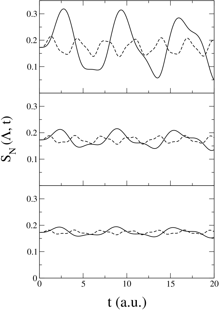
Figure 2: Information-theoretic, von Neumann, entropies $S_{N}(\Lambda,t)$, as a function of the time $t$, which is measured in atomic units. The solid and dashed curves refer to a moderate interparticle repulsion $\Lambda=0.3$, and the corresponding (see the text) interparticle attraction $\Lambda=-0.75$, respectively. Three values for the rate parameter $\beta$, measured in inverse time-units, are employed to illustration. Top panel: $\beta=2$. Middle panel: $\beta=5$. Bottom panel: $\beta=10$.

In Figure 2 we exhibit $S_{N}(\Lambda,t)$, by taking $\omega_{0}=1$, $Q=0.2$, $\Lambda=0.40$ and $\Lambda=-2.0$. These couplings for repulsion and attraction, respectively, are fixed to yield equal entropies at $t=0$, in order to shed further light on duality Pipek09 ; Glasser13 ; Schilling14 , now in the time-domain as well. Notice, that in the unperturbed case to any allowed [$\Lambda\in(0,0.5)]$ repulsive coupling there exists a corresponding attractive ($\Lambda<0$) one for which the calculated entropies are equal. For instance, when we are close to the stability limit in the repulsive ($r$) case, i.e., when $\Lambda_{r}\rightarrow{0.5}$, the corresponding attractive ($a$) coupling becomes $\Lambda_{a}\rightarrow{(1/2)(2\Lambda_{r}-1)^{-1}}$.

The solid and dashed curves refer to repulsion and attraction, as we mentioned. They are plotted as a function of the time measured in atomic units. The rate-parameter of the time-dependent external perturbation is described by $\beta$ and measured in inverse units of time. In order to discuss tendencies, we used three values for this parameter. As expected, at very short times the entropies, similarly to the energy changes, grow in time. After about 1-2 atomic units (i.e., about 25-50 attoseconds) they start to reflect the oscillating character builded into the time-dependent occupation numbers $P_{l}(t)$, the primary root of which is in the time-evolving correlated wave function. The entropies will keep, in absence of an environment-made dissipative Albrecht75 ; Tokatly13 coupling, such oscillating behavior without limitation. From this point of view, they signal the time-evolvement of the closed interacting system. More importantly, one can see from the illustration that the initial dual character of entropies, fixed at $t=0$, will disappear due to a new physical variable, i.e., the time. Finally, there are reductions in the oscillation-amplitudes by increasing $\beta$. Clearly, at the so-called sudden limit ($\beta\rightarrow{\infty}$) for a time-dependent perturbation, they will diminish as expected, since the system’s reaction-rapidity is limited by its normal mode frequencies.

In order to justify the above argument more directly, we take now a somewhat less realistic modeling by using an abrupt quench of all interactions at $t_{0}=0$ in the Hamiltonian. In that case, instead of Eqs. (33-34), one gets Kagan96 the following exact expressions

$$R_{i}(\Lambda,\omega_{i},t)\,=\,\sqrt{1+t^{2}\,\omega_{i}^{2}}$$ (36)

$$\dot{R}_{i}(\Lambda,\omega_{i},t)\,=\,\frac{t\,\omega_{i}^{2}}{\sqrt{1+t^{2}\,\omega_{i}^{2}}}.$$ (37)

There is no change in the system’s kinetic energy since $[1/R_{i}(\omega_{i},t)]^{2}+[\dot{R}_{i}(\omega_{i},t)/\omega_{i}]^{2}=1$. By using time-dependent $A(t)$ and $\omega_{s}(t)$, which are needed to Eq. (25), we get $z(t)=z(t=0)$ for all $t\geq{0}$ since $[\omega_{s}(t)/A(t)]\equiv{2[2\sqrt{\omega_{1}\omega_{2}}/(\omega_{1}-\omega_{2})]^{2}}$. Thus, there is no entropy-change in the total-quench case. This $S(t)=constant$ character could be a useful constraint in practical attempts, with a good starting $n(x,t)$, using the interconnected $z_{d}(t)$ and $\omega_{d}(t)$ variables of Eq. (28). One can take $\omega_{d}(t)\Rightarrow{\omega_{d}/R^{2}(\omega_{d},t)}$, where $R(\omega_{d},t)=\sqrt{1+t^{2}\omega_{d}^{2}}$.

III summary and comments

Based on the time-dependent Schrödinger equation, an exact calculation is performed for the time-evolving energy change, and orthogonality of initial and final states, in a correlated two-particle model system driven by a weak external field of quadrupolar character. Besides, considering the structure of the exact time-dependent one-matrix, an independent-particle model is defined from it which contains exact information on the single-particle probability density and probability current. The resulting noninteracting auxiliary state is used to construct an effective potential and discuss its applicability. We analyzed the energy changes in a comparative manner, and pointed out (see, below as well) the limited capability of an optimized independent-particle modeling for the underlying time-dependent process.

A point-wise decomposition of the reduced one-particle density matrix is given in terms of time-dependent occupation numbers and time-dependent orthonormal orbitals. Based on such exact spectral decomposition on the time domain, an entropic measure of inseparable correlation is also investigated. It is found that the duality behavior characterizing the stationary ground-state may disappear depending on the rapidity of the external time-dependent perturbation. At realistic rapidity, the undamped time-dependent oscillations, found in an entropic measure, reflect the fact that the correlated system evolves in time. In this respect, we have a signal on the excited state, similarly as one can see in the time-evolving probability density and probability current.

Our first comment is based on results obtained for the energy changes, and plotted in Figure 1, by considering the sign of $\Lambda$. In the case of an attractive interparticle interaction, the case of a nucleus Moshinsky68 , the exact result for $\Delta E(\Lambda<0,\beta,t)$ becomes bigger at moderate $\beta$ values than the result obtained within the density-optimal framework $\Delta E_{e}(\Lambda<0,\beta,t)$. So, we speculate that a recent result Stetcu15 on the excitation of a deformed nucleus within TD-DFT could have the same, underestimating character in its quadrupole channel, as the atomistic case has. Thus, the true enhancement in excitations over the result based on the modeling of Teller Teller48 , might also need further theoretical refinement for that channel.

In the second comment, we focus on the role of the switching rate $\beta$ in the case of energy changes. As a preliminary step to future realistic calculations, here we would like to estimate a characteristic interaction-time ($T\propto{\beta^{-1}}$) in classical atom-atom collision. To do that, we model the three-dimensional screened interaction via a finite-range ($r\leq{R}$) potential

$$V(r)\,=\,\frac{Z_{1}\,Z_{2}\,e^{2}}{r}\left(1-\frac{r}{R}\right).$$ (38)

Solving the classical problem Nagy94 for the collision time ($T$) we get

$$T(b,v,R)=\frac{2}{v}\left[\frac{\sqrt{R^{2}-b^{2}}}{c}+\frac{Z_{1}Z_{2}e^{2}}{2E_{1}}\frac{1}{c^{3/2}}\ln\frac{\sqrt{c}\sqrt{R^{2}-b^{2}}+R+(Z_{1}Z_{2}e^{2}/2E_{1})}{\sqrt{(Z_{1}Z_{2}e^{2}/2E_{1})^{2}+c\,b^{2}}}\right]$$ (39)

where $E_{1}=M_{1}v^{2}/2$ is the energy of a heavy charged ($Z_{1}e$) projectile moving with velocity $v$ and colliding at impact parameter $b$ with a fixed center of effective charge $Z_{2}e$. The dimensionless parameter introduced is $c=[1+(Z_{1}Z_{2}e^{2}/R)/E_{1}]$, i.e., it is related to the ratio of potential and kinetic energies. A closer inspection of this compact (and reasonable at short-range solid-state conditions) form shows that practically one may use

$$T(b,v,R)\,\simeq{\alpha(v)\,\frac{R}{v}\,\frac{E_{1}}{E_{1}+Z_{1}Z_{2}e^{2}/R}}\,\sqrt{1-\frac{b^{2}}{R^{2}}}$$ (40)

to get a very acceptable estimation as a function of the heavy projectile velocity $v$, with which $\alpha(v)$ is decreasing from 4 (at $v\rightarrow{0}$) to 2 (at $v\rightarrow{\infty}$). If we take $\beta(v)\simeq{T^{-1}(v)}$ and consider the energy change determined above, we get a $\Delta E(v)\sim{[\beta(v)]^{-2}}\sim{[\alpha(v)v]^{2}}$ character at very low velocities. For the opposite, high-velocity, limit $\Delta E(v)\sim{[\beta(v)]^{-2}}\sim{[\alpha(v)v]^{-2}}$ is the scaling, which also looks quite reasonable physically. However, the detailed work on the exactly determined non-linear energy changes is left for a dedicated publication.

There, and also in Bohr’s pioneering modeling Bohr13 ; Merzbacher74 with time-dependent dipole fields of a passing charge, the time-scale derived above using collision theory, could play a more quantitative role to understand fine details behind experimental predictions Moller04 ; Markin09 on energy losses of slow ions in insulators. Furthermore, in the renewed field of time-dependent energy losses, a proper time-scale also could help to analyze further a remarkable theoretical prediction Correa12 on the strong interplay of nuclear and electronic stopping components of the observable total energy transfer. Indeed, few-electron shake-up processes can be dominant at close encounters in condensed matter. In such dynamical cases, one-electron approximations, with double-occupancy for an auxiliary spatial orbital, could result in inaccuracies.

- (1) W. Heisenberg, Z. Phys. 38, 411 (1926).
- (2) M. Moshinsky, Am. J. Phys. 36, 52 (1968).
- (3) L. E. Ballentine, Quantum Mechanics (World Scientific, Singapore, 1998).
- (4) V. S. Popov and A. M. Perelomov, Sov. Phys. JETP 30, 910 (1970).
- (5) Yu. Kagan, E. L. Surkov, and G. V. Shlyapnikov, Phys. Rev. A 54, R1753 (1996).
- (6) A. del Campo, Phys. Rev. Lett. 111, 100502 (2013).
- (7) E. Fermi, Phys. Rev. 57, 485 (1940).
- (8) N. Bohr, Phil. Mag. 25, 10 (1913).
- (9) J. F. Dobson, Phys. Rev. Lett. 73, 2244 (1994).
- (10) M. Brics and D. Bauer, Phys. Rev. A 88, 052514 (2013).
- (11) C. R. McDonald, G. Orlando, J. W. Abraham, D. Hochstuhl, M. Bonitz, and T. Brabec, Phys. Rev. Lett. 111, 256801 (2013).
- (12) H. Kohl and R. M. Dreizler, Phys. Rev. Lett. 56, 1993 (1986).
- (13) C. A. Ullrich, Time-Dependent Density-Functional Theory (Oxford University Press, Oxford, 2012), and references therein.
- (14) M. Ruggenthaler, M. Penz, and R. van Leeuwen, arXiv: 1412.7052v1 [cond-mat.other].
- (15) J. Schirmer and A. Dreuw, Phys. Rev. A 75, 022513 (2007).
- (16) J. Pipek and I. Nagy, Phys. Rev. A 79, 052501 (2009).
- (17) Ch. Schilling, D. Gross, and M. Christandl, Phys. Rev. Lett. 110, 040404 (2013).
- (18) M. L. Glasser and I. Nagy, Phys. Lett. A 377, 2317 (2013).
- (19) Ch. Schilling and R. Schilling, J. Phys. A: Math. Theor. A 47, 415305 (2014).
- (20) D. W. Robinson, Nucl. Phys. 25, 459 (1961).
- (21) K. W. Hill and E. Merzbacher, Phys. Rev. A 9, 156 (1974).
- (22) M. Mierzejewski and P. Prelovsek, Phys. Rev. Lett. 105, 186405 (2010).
- (23) M. Lein and S. Kümmel, Phys. Rev. Lett. 94, 143003 (2005).
- (24) I. Nagy, Phys. Rev. A 87, 052512 (2013).
- (25) A. Erdélyi, Higher Transcendental Functions (McGraw-Hill, New York, 1953), p. 194.
- (26) P. Koscik, Phys. Lett. A 379, 293 (2015).
- (27) J. Rapp, M. Brics, and D. Bauer, Phys. Rev. A 90, 012518 (2014).
- (28) C. L. Benavides-Riveros and I. Nagy, arXiv: 1406.2809v1 [quant-ph].
- (29) A. Rényi, Probability Theory (North-Holland, Amsterdam, 1970).
- (30) P. Calabrese, P. Le Doussal, and S. N. Majumdar, Phys. Rev. A 91, 012303 (2015).
- (31) M. Ashan Zeb, J. Kohanoff, D. Sánchez-Portal, and E. Artacho, Nucl. Instrum. Methods Phys. Res. B 303, 59 (2013).
- (32) F. Mao, Ch. Zhang, J. Dai, and R.-S. Zhang, Phys. Rev. A 89, 022707 (2014).
- (33) K. Albrecht, Phys. Lett. 56B, 127 (1975), and references therein.
- (34) I. V. Tokatly, Phys. Rev. Lett. 110, 233001 (2013).
- (35) I. Stetcu, C. A. Bertulani, A. Bulgac, P. Magierski, and K. J. Roche, Phys. Rev. Lett. 114, 012701 (2015).
- (36) M. Goldhaber and E. Teller, Phys. Rev. 74, 1046 (1948).
- (37) I. Nagy, Nucl. Instrum. Methods Phys. Res. B 94, 377 (1994).
- (38) S. P. Moller, A. Csete, T. Ichioka, H. Knudsen, U. I. Uggerhoj, and H. H. Anderson, Phys. Rev. Lett. 93, 042502 (2004), and references therein.
- (39) S. N. Markin, D. Primetzhofer, and P. Bauer, Phys. Rev. Lett. 103, 113201 (2009).
- (40) A. A. Correa, J. Kohanoff, E. Artacho, D. Sánchez-Portal, and A. Caro, Phys. Rev. Lett. 108, 213201 (2012), and references therein.