Photohadronic origin of -ray BL Lac emission: implications for IceCube neutrinos
Abstract
The recent IceCube discovery of PeV neutrinos of astrophysical origin opens up a new era for high-energy astrophysics. Although there are various astrophysical candidate sources, a firm association of the detected neutrinos with one (or more) of them is still lacking. A recent analysis of plausible astrophysical counterparts within the error circles of IceCube events showed that likely counterparts for nine of the IceCube neutrinos include mostly BL Lacs, among which Mrk 421. Motivated by this result and a previous independent analysis on the neutrino emission from Mrk 421, we test the BL Lac-neutrino connection in the context of a specific theoretical model for BL Lac emission. We model the spectral energy distribution (SED) of the BL Lacs selected as counterparts of the IceCube neutrinos using a one-zone leptohadronic model and mostly nearly simultaneous data. The neutrino flux for each BL Lac is self-consistently calculated, using photon and proton distributions specifically derived for every individual source. We find that the SEDs of the sample, although different in shape and flux, are all well fitted by the model using reasonable parameter values. Moreover, the model-predicted neutrino flux and energy for these sources are of the same order of magnitude as those of the IceCube neutrinos. In two cases, namely Mrk 421 and H 1914-194, we find a suggestively good agreement between the model prediction and the detected neutrino flux. Our predictions for all the BL Lacs of the sample are in the range to be confirmed or disputed by IceCube in the next few years of data sampling.
keywords:
astroparticle physics – neutrinos – radiation mechanisms: non-thermal – galaxies: BL Lacertae objects: individual: Mrk 421, 1ES 1011+496, PG 1553+113, H 2356309, 1H 1914194, 1RXS J054357.35532061 Introduction
During the first three years of data sampling in full configuration, the IceCube Neutrino Telescope based at the South Pole has registered a sample of very high-energy neutrinos (30 TeV – 2 PeV) of astrophysical origin (Aartsen et al., 2013, 2014). With a sample of 37 events the background only hypothesis with no astrophysical component has been rejected with a significance of more than 5 . A new era for high-energy astrophysics just started.
Excluding, in this context, the possible connection with dark matter (Cherry et al., 2014; Esmaili et al., 2014), the IceCube discovery calls for astrophysical sites, where cosmic-ray acceleration at the “knee” energy scale and above is efficiently at work, and the target, be it gas or photons, is sufficiently dense for interactions with the cosmic rays. A firm association between the detected neutrinos and a specific class (or classes) of astrophysical sources is still lacking, notwithstanding the numerous scenarios that have been proposed so far. Models suggesting a pure Galactic origin of the observed neutrino signal can be strongly constrained by diffuse TeV-PeV -ray limits (see e.g. Ahlers & Murase 2014; Joshi et al. 2014 and references therein), given that the production of very high energy (VHE) -rays is an inevitable outcome of the hadronic interactions that lead to the neutrino production in the first place. However, a Galactic component contributing to the IceCube neutrino flux cannot be excluded at the moment. Proton-proton () collisions in galaxy groups and/or star forming galaxies have also been invoked to explain the diffuse neutrino flux (e.g. Loeb & Waxman 2006; Murase et al. 2013). Other extragalactic scenarios that include neutrino production through photohadronic () interactions in active galactic nuclei (AGN) (Stecker et al., 1991; Mannheim, 1995; Halzen & Zas, 1997; Rachen & Mészáros, 1998; Mücke et al., 1999; Atoyan & Dermer, 2001; Mücke et al., 2003) and gamma-ray bursts (GRBs) (Waxman & Bahcall, 1997; Murase, 2008; Zhang & Kumar, 2013; Asano & Mészáros, 2014; Reynoso, 2014; Petropoulou et al., 2014; Winter et al., 2014) have been extensively discussed in the literature.
A commonly adopted approach for the calculation of the neutrino flux at Earth (see e.g. Mannheim et al. 2001; Baerwald et al. 2013; Kistler et al. 2013; Murase et al. 2014) is the following: (i) a generic distribution of accelerated protons in the source is assumed; (ii) a generic photon distribution that acts as a target field for interactions is also assumed; (iii) the neutrino spectrum is then calculated; and (iv) the neutrino flux is integrated over redshift assuming a luminosity function for the particular astrophysical source. If many sources of the same type contribute to the observed flux, then the approach described above is the most relevant one. A different approach is to focus on a few individual sources of the same class and derive the respective neutrino fluxes using proton and photon distributions that are unique to each object (Mücke et al., 2003; Dimitrakoudis et al., 2014). In this regard, information about the directions of the neutrino events on the sky is important. This approach may still lead to a study of the diffuse neutrino flux, from a certain class of sources, but with the caveat that it may not represent the total diffuse flux; the latter could be arrived at only upon an estimate of the percentage of that class’s contribution to the total.
Padovani & Resconi (2014) – henceforth PR14, have recently searched for plausible astrophysical counterparts within the error circles of IceCube neutrinos using high-energy -ray (GeV-TeV) catalogs. Assuming that each neutrino event is associated with one astrophysical source and using a model-independent method they derived the most probable counterparts for 9 out of the 18 neutrino events of their sample. Interestingly, these include 8 BL Lac objects, amongst which the nearest blazar, Mrk 421, and two pulsar wind nebulae. Although Flat Spectrum Radio Quasars (FSRQs) are believed to be more efficient PeV neutrino emitters than BL Lacs (e.g. Dermer et al. 2014; see, however, Tavecchio et al. (2014)), these do not appear in the list of most probable counterparts. This is not necessarily related to the physics of neutrino emission from different types of blazars but could be a consequence of the “energetic” test applied by PR14 (for more details, see §4 therein).
Motivated by the aforementioned results, we investigate the BL Lac–PeV neutrino connection within a specific theoretical framework for blazar emission where the -rays are of photohadronic origin. In contrast to the majority of works on neutrino emission from blazars, we do not assume a generic SED but we fit instead the multiwavelength (MW) photon spectra using the radiation of particles whose distributions have been accordingly modified by the cooling and escape processes. In our model the low-energy emission of the blazar SED is attributed to synchrotron radiation of relativistic electrons, whereas the observed high-energy (GeV-TeV) emission is the result of synchrotron radiation from pairs produced by charged pion decays. Pions are the by-product of interactions of co-accelerated protons with the internally produced synchrotron photons. Our approach allows us to identify the observed -ray emission as the emission from the component and associate it with a very high-energy ( PeV) neutrino emission. Analytical expressions for the typical energies of neutrinos and photons produced through photohadronic processes, the proton cooling rate due to photopion and photopair interactions, as well as the dependence of all aforementioned quantities on observable quantities of blazar emission can be found in Petropoulou & Mastichiadis (2015).
First results of the model were presented in Dimitrakoudis et al. (2014) – henceforth DPM14, where the neutrino flux expected from the prototype blazar Mrk 421 in a low state was derived. The prediction of the model muon neutrino flux was tantalizingly close to the IC-40 sensitivity limit calculated by Tchernin et al. (2013) for Mrk 421 (see Fig. 1 in DPM14). We extend our previous analysis to include those BL Lacs identified as the most probable counterparts of the IceCube neutrinos by PR14 (see Table 4 therein). Our aim is threefold: (i) to examine whether the working model (the so-called LH model, see DPM14) can fit the SED of the aforementioned blazars – there was no guarantee before our attempts, since we did not select a priori sources with specific spectral characteristics; (ii) to calculate the neutrino flux relative to the -ray one, should acceptable fits be obtained, and (iii) to compare the model-derived neutrino fluxes with those calculated for each single neutrino event. We show that Mrk 421 does not constitute a unique case. Instead, all BL Lacs in our sample can be modelled by the leptohadronic model and for most of them the model-predicted neutrino flux is close to the observed one, at least within the error bars.
This paper is structured as follows. We start with a short description of the theoretical model and the fitting method we used in Sect. 2. In Sect. 3 we provide general information about the observational datasets used for each BL Lac. In Sect. 4 we present the combined MW photon and neutrino spectra for each of the case studies, focusing on the ratio of the model-predicted neutrino luminosity to the -ray luminosity and its dependence on observable quantities. We also comment on the model-derived energetics for each source. We discuss our results in Sect. 5 and conclude with a summary in Sect. 6. Throughout this work we have adopted a cosmology with , and km s-1 Mpc-1. For the attenuation of the VHE part of the spectra due to photon-photon pair production on the extragalactic background light (EBL) we used the model of Franceschini et al. (2008).
2 Model and method
2.1 Model description
The physical model we use has been described, in general terms, in Dimitrakoudis et al. (2012) - henceforth DMPR12, and, in the context of modelling Mrk 421 in particular, in Mastichiadis et al. (2013) and DPM14. We consider a spherical blob of radius , containing a tangled magnetic field of strength B and moving towards us with a Doppler factor . Protons and electrons are accelerated by some mechanism whose details lie outside the immediate scope of this work, and are subsequently injected isotropically in the volume of the blob with a constant rate. Their interaction with the magnetic field and with secondary particles leads to the development of a system where five stable particle populations are at work: protons, which lose energy by synchrotron radiation, Bethe-Heitler (pe) pair production, and photopion () interactions; electrons (including positrons), which lose energy by synchrotron radiation and inverse Compton scattering; photons, which gain and lose energy in a variety of ways; neutrons, which can escape almost unimpeded from the source region, with a small probability of photopion interactions; and neutrinos, which escape completely unimpeded.
The interplay of the processes governing the evolution of the energy distributions of those five populations is formulated with a set of time-dependent kinetic equations. Through them, energy is conserved in a self-consistent manner, since all the energy gained by a particle type has to come from an equal amount of energy lost by another particle type. To simultaneously solve the coupled kinetic equations for all particle types we use the time-dependent code described in DMPR12. Photopion interactions are modelled using the results of the Monte Carlo event generator SOPHIA (Mücke et al., 2000), while Bethe–Heitler pair production is similarly modelled with the Monte Carlo results of Protheroe & Johnson (1996) and Mastichiadis et al. (2005). The only particles not modelled with kinetic equations are muons, pions and kaons. Their treatment is described in DPM14 and Petropoulou et al. (2014) but is of negligible importance for the range of parameter values used in the present work.
The prime mover of all processes is the rate at which energy is injected in relativistic protons and electrons. This, in terms of compactnesses, is expressed as:
| (1) |
where i denotes protons or electrons (i=e,p), is the Thomson cross section, and denotes the injection luminosity as measured in the rest frame of the emitting region. In principle, the radius and Doppler factor can be constrained using variability arguments. However, we prefer to treat them as free parameters, since information for high-energy variability is not available for all sources in the sample. The escape times for protons and electrons are assumed to be the same (), and complete the set of free parameters dependent on the geometry and kinematics of the blob. What remains to be defined are the shapes of the proton and primary electron injection functions, which are described as power-laws with index extending from to . In some cases, modelling of the SED requires the primary electron distribution to be a broken power-law, with the break energy and the power-law index above the break being two additional free parameters.
As long as the escaping protons and neutrons are energetic enough, they are susceptible to photopion interactions with ambient photons in Galactic and intergalactic space, such as the cosmic microwave and infrared backgrounds, producing additional high-energy neutrinos (Stecker, 1973). Neutrons also rapidly decay into protons (Sikora et al., 1987; Kirk & Mastichiadis, 1989; Giovanoni & Kazanas, 1990; Atoyan & Dermer, 2001), leading also to neutrino production. In this work we focus on the neutrino emission from the objects themselves, and will not consider any such additional contributions from escaping high-energy nucleons.
The reader should note that we placed our emphasis on fitting the MW data with a variant of the leptohadronic model where the -ray emission is attributed to synchrotron radiation of the secondaries arising from charged pion decay. Clearly, this is not the only way of fitting the SED, as it is possible to fit the -rays with proton synchrotron radiation (e.g. Aharonian 2000). In that case, however, the model produces a very low neutrino flux at EeV energies (see LHs model in DPM14), which makes it irrelevant to the IceCube TeV-PeV detections. Moreover, scenarios where the high-energy blazar emission is the result of -rays produced through collisions within the blazar jet, constitute another alternative111 To our knowledge, direct application of such models to MW observations of blazars is still lacking in the literature.. Such models would require, however, uncomfortably high densities of non-relativistic (cold) protons to be present in the blazar jet (see e.g. Atoyan & Dermer 2004 and references therein). Last but not least, there is always the possibility of assuming a purely leptonic model (Böttcher et al., 2013) which, however, does not produce any neutrinos.
2.2 Fitting method
The multi-parameter nature of the problem (11-13 free parameters; see Sect. 4) and the long simulation time, which is required for every parameter set (of the order of d), prevents us from a blind search of the whole available parameter space. Moreover, the DMPR12 code in its current form has not been developed for parallel computing. Yet, the application of the model to actual observations is still viable (e.g. Mastichiadis et al. 2013; Petropoulou 2014) thanks to the insight we gain from an analytical treatment of the problem. Thus, instead of automatically scanning the parameter space, we start the fitting procedure with a set of values, which are physically motivated (see below). Then, we perform a series of numerical simulations with parameter values lying close to the initial parameter set, until a reasonably good fit to the SED is obtained. The term “reasonably good” fit refers to a model SED that passes through most observational points. This is not necessarily the best fit in the strict sense, i.e. the one with the lowest value. However, the main results of our study, such as the -ray/neutrino connection, are not affected by the exact value of the statistics.
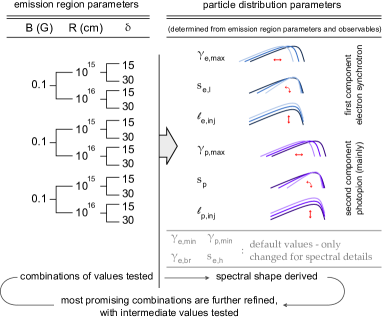
The steps of the fitting method are illustrated in Fig. 1. The parameters of the problem can be divided into two groups; those related to the properties of the emission region, i.e. , and and those related to the primary particle distributions (see two columns in Fig. 1). As benchmark values for the magnetic field we chose G. These cover the range of low-to-moderate magnetic fields. Higher values, e.g. G, were not included to the benchmark set, since they tend to favour proton synchrotron radiation against photohadronic processes (for proton synchrotron models, see Aharonian 2000; Mücke et al. 2003; Böttcher et al. 2013; Dimitrakoudis et al. 2014; Cerruti et al. 2014). For each value of , we then adopted cm and cm and the set of benchmark values is completed with and . We did not search in the first place for fits having even higher values of and , since they would decrease the optical depth () for photopion interactions and for neutrino production. If the low-energy hump of the SED has peak spectral index , peak frequency and total luminosity the optical depth for neutrino production is given by (e.g. PM15)
| (2) |
where we introduced the notation in cgs units, is a function of and (see equations (23) and (27) in PM15), is the redshift of the source, is the low cutoff frequency of the low-energy spectrum (for a continuous power-law), is the proton Lorentz factor and is the minimum Lorentz factor that satisfies the threshold condition for interactions with the peak energy photons. This is given by (for details, see PM15)
| (3) |
Protons with the aforementioned Lorentz factor lead to the production of neutrinos with energy, as measured in the observer’s frame, given by
| (4) |
In most cases, the above expressions is a safe estimate of the peak energy of the neutrino spectrum.
We use equation (3) as the minimum requirement for the maximum proton energy of the proton distribution, i.e. with a numerical factor of . On the other hand, the maximum (or break) Lorentz factor of the primary electron distribution is related to the peak frequency of the low-energy hump as
| (5) |
For the lower cutoffs of the proton and primary electron injection functions we use as default values (grey colored parameters in Fig. 1). If we find large deviations of the model SED from the observations at , we search for . We search for different than the default one only if the proton distribution has and extension to leads to extremely high injection luminosities. We note, however, that this is not a typical case.
The power-law index of the primary electron distribution ( or ) is directly related to the observed spectral index of the low-energy component in the SED. However, it is not straightforward to relate with the observed photon index, e.g. in the Fermi/LAT regime, where the emission from secondaries produced in photohadronic interactions dominates. Thus, as a first estimate we use .
The injection luminosity of primary electrons is also directly related to the observed luminosity of the low-energy hump as (e.g. Mastichiadis & Kirk 1997)
| (6) |
To derive a first estimate of the proton injection luminosity we assume that the -ray ( GeV) luminosity is totally explained by the synchrotron emission of pairs:
| (7) | |||||
| (8) |
where is given by equation (2). The factor in equation (8) comes from the assumption that half of the produced pions produce electrons/positron pairs, and each of them gains of the parent proton energy:
| (9) |
The characteristic photon energy is given by
| (10) |
where
| (11) |
Using equations (7)-(11), (1), and (2) we derive a rough estimate of the proton injection compactness:
| (12) |
Summarizing, for each set of benchmark values for and and equipped with the analytical estimates of equations (2)-(12) and observables, we may significantly reduce the parameter space we need to scan (Fig. 1).
3 Case studies
Our modelling targets are BL Lacs that are spatially and energetically correlated with neutrino detections. BL Lacs are known for their variable emission at almost all energies. In high-states they usually exhibit major flares, especially in X-rays and -rays. Modelling of their broadband emission in low and high states requires a different parameterization. For example, a high-flux state might need a stronger magnetic field (for modelling of blazar flares, see Mastichiadis & Kirk 1997; Coppi & Aharonian 1999; Sikora et al. 2001; Krawczynski et al. 2002), which in turn would affect the resulting -ray and neutrino fluxes. Thus, it is important to build an SED using simultaneous data or, if this is not possible, using MW observations that have been obtained at least within the same year.
Out of the 8 BL Lacs reported by PR14, two have unknown redshifts: SUMSS J014347-584550 and PMN J0816-1311, which are the probable counterparts of neutrinos 20 and 27, respectively. Since redshift is a crucial parameter in determining the luminosity of the emitting regions and, thus, the interplay of processes at work there, we have chosen to exclude those two BL Lacs from this study. Therefore, we are left with six targets, which are:
-
•
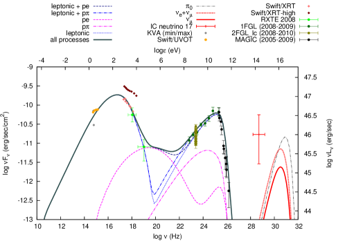
Mrk 421 at (Sbarufatti et al., 2005). This is the closest high-frequency peaked blazar (HBL) and the target of many MW campaigns. Mrk 421 was also the first source which our model (see Sect. 2.1) was applied to and the main focus of an earlier work (DPM14). We first quote the results of DPM14, that used the simultaneous X-ray (RXTE) and TeV -ray (Whipple and HEGRA) data of the 2001 MW campaign that lasted 6 days (Fossati et al., 2008). In particular, DPM14 fitted the SED of March 22nd/23rd 2001 that corresponds to a pre-flare state. During this period no GeV observations were available. Thus, the Fermi/LAT data during the period of the IC-40 configuration (Abdo et al., 2011) were included for comparison reasons only. As a second step, we use the MW observations of Abdo et al. (2011) together with the neutrino event ID 9 in order to build a hybrid SED. To avoid repetition and to emphasize the prediction of DPM14 regarding the muon neutrino flux, we do not attempt to fit the new dataset. Instead, we use the same parameters as in DPM14, apart from the Doppler factor, and compare the model results against the Abdo et al. (2011) observations and the neutrino flux for the event ID 9.
-
•
PG 1553+113 at (Aleksić et al., 2012). This is not only the most distant source of this sample, but also belongs to the class of most distant TeV blazars in general. Its redshift has not been firmly measured, yet the value adopted here can be considered as a safe estimate (for different techniques and results, see Aleksić et al. 2012). Similarly to 1ES 1011+496 below, it has been only recently detected in VHE -rays by both H.E.S.S. (Aharonian et al., 2006b) and MAGIC (Albert et al., 2007a). The data from the second year Fermi-LAT Sources Catalog at GeV (2FGL_lc) 222http://www.asdc.asi.it/fermi2fgl/ indicate a variable high-energy flux. The 2005-2009 MAGIC observations also suggest variability at the VHE part of the spectrum (see Fig. 1 in Aleksić et al. 2012). In 2005 the source exhibited large flux variations in X-rays, yet there were no simultaneous data, neither at GeV nor at TeV energies. We adopted the data shown in Fig. 6 of Aleksić et al. (2012). For the SED fitting we used, in particular, the X-ray data that correspond to the intermediate flux level of 2005 along with the time-averaged 2008-2009 Fermi/LAT data and the MAGIC observations for the periods 2005-2006 and 2007-2009. We include in our figures the high state X-ray data of 2005 only for illustrative reasons. In principle, one could try to fit the time-averaged -ray data together with the 2005 high state in X-rays. However, we find less plausible a scenario where the 2005 X-ray high-state is not accompanied by an increased -ray flux but, instead, is related to the average -ray flux level. There are two reasons for this: the -ray and X-ray emission in blazars are usually correlated (e.g. for Mrk 421, see Fossati et al. 2008) and the -ray emission of PG 1553+113 is itself variable (see e.g. Aharonian et al. 2006b).
-
•
1ES 1011+496 at (Albert et al., 2007b). This is an HBL source at indermediate redshift, that has been detected for the first time in TeV -rays in 2007 with MAGIC (Albert et al., 2007b). The discovery was the result of a follow up observation of the optical high state reported by the Tuorla blazar monitoring program333http://users.utu.fi/kani/1m. The previous non-detections in TeV -rays suggest that 1ES 1011+496 is variable both in optical and VHE -rays. Its X-ray emission is described by a steep spectrum in both low and high states (see Reinthal et al. 2012 and references therein). Because of the variability observed across the MW spectrum, we chose to apply our model to simultaneous data, if possible. We therefore used data from the first MW campaign in 2008 as presented in Reinthal et al. (2012), despite the fact that they are characterized as preliminary. We note that the MAGIC data presented in Reinthal et al. (2012) have been de-absorbed using the EBL model of Kneiske & Dole (2010). Using the same model we retrieved the observed MAGIC spectrum, which we show in the respective figure. We also took into account the Fermi/LAT data from the first (1FGL) (Abdo et al., 2010) and second (2FGL) (Nolan et al., 2012) catalogs. In the respective figures we include 2FGL_lc data, in order to show the variability in the GeV regime.
-
•
H 2356-309 at (Falomo, 1991). This is one of the brightest HBLs in X-rays, which led to its early X-ray detection with UHURU (Forman et al., 1978). Its X-ray emission is variable both in flux and in spectral shape (for more information, see H.E.S.S. Collaboration et al. 2010). TeV -ray emission from H 2356-309 was observed for the first time in 2004 by H.E.S.S. (Aharonian et al., 2006a). Using the SED builder tool444http://www.asdc.asi.it/SED of the ASI Science Data Centre (ASDC) we chose those X-ray observations that fall within the period 2004-2007 of H.E.S.S. observations. We also included data from the 1FGL and 2FGL catalogs, although they refer to the period 2008-2010, as well as hard X-ray data obtained by Swift/BAT between 2004 and 2010. Finally, we over-plotted the historical X-ray high state observed with BeppoSaX, for comparison reasons.
-
•
1H 1914-194 at (Carangelo et al., 2003). This is the first BL Lac of the sample that has not yet been detected in TeV -rays, and the least well covered in different energy bands among the sources of this sample. In order to apply our model we constructed a SED using available data from the ASDC, which is comprised mainly of NED archival data. Given the quality of the available dataset, our main focus was to describe as well as possible the Fermi/LAT data, while roughly describing the observations in other energy bands.
-
•
1 RXS J054357.3-553206 at (Stadnik & Romani, 2014). This is the second most distant object of the sample, after blazar PG 1553+113. It was first detected and classified as a BL Lac by ROSAT (Fischer et al., 1998). Following radio observations by Anderson & Filipovic (2009) it was classified as an HBL, and it was soon thereafter detected in -rays by Fermi/LAT (Abdo et al., 2010). It remains still undetected in TeV energies. Its redshift was estimated by Stadnik & Romani (2014), based on the assumption that the flux of the host elliptical galaxies of BL Lacs can be used as a standard candle, and also by Pita et al. (2014), based on spectroscopy on a weak Ca II H/K doublet and a Na I absorption line. While the Pita et al. (2014) estimate () is somewhat lower than the Stadnik & Romani (2014) one, adopting it would not significantly alter out fit. Using the SED builder tool of ASDC we combined infrared (WISE), X-ray (Swift/XRT and XMM-Newton) and -ray (Fermi/LAT) observations that were obtained within the same year (2010). We also included older XMM-Newton observations performed in 2005 and 2007, for comparison reasons. Finally, the 2FGL_lc data illustrate the variability in the GeV energy band.
Before closing this section and for completeness reasons, we summarize in Table 1, the coordinates of the five IceCube neutrinos and the six most probable blazar counterparts, as well as their angular offset. We also included the median angular error for each neutrino detection and the respective detection time in Modified Julian Days (MJD)555We note that all data listed in Table 1 are adopted from Tables 1 and 2 in PR14.. A sky map (in equatorial coordinates) of the five IceCube neutrinos and their respective counterparts is shown in Figure 2.
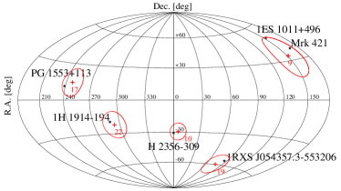
| IceCube ID | Ra(deg) | Dec(deg) | Median angular error (deg) | Time (MJD) | Counterpart | Ra(deg) | Dec(deg) | Angular offset (deg) |
|---|---|---|---|---|---|---|---|---|
| 9 | 151.25 | 33.6 | 16.5 | 55685.6629638 | Mrk 421 | 166.08 | 38.2 | 12.8 |
| 1ES 1011+496 | 155.77 | 49.4 | 15.9 | |||||
| 10 | 5.00 | -29.4 | 8.1 | 55695.2730442 | H 2356-309 | 359.78 | -30.6 | 4.7 |
| 17 | 247.40 | 14.5 | 11.6 | 55800.3755444 | PG 1553+113 | 238.93 | 11.2 | 8.9 |
| 19 | 76.90 | -59.7 | 9.7 | 55925.7958570 | 1RXS J054357.3-553206 | 85.98 | -55.5 | 6.4 |
| 22 | 293.70 | -22.1 | 12.1 | 55941.9757760 | 1H 1914-194 | 289.44 | -19.4 | 4.8 |
4 Results
We first present the results of our SED modelling along with the predicted neutrino flux for each source, i.e. we build model hybrid SEDs. The parameter values derived for each source are summarized in Table 2. Various aspects of the adopted theoretical framework were investigated in detail in a recent work (Petropoulou & Mastichiadis 2015 – hereafter PM15). For details and analytical expressions that give insight to the results that follow, we refer the reader to PM15. In the last two subsections we discuss in more detail the neutrino emission and the energetics for each source.
| Parameter | Mrk 421 | PG 1553+113 | 1ES 1011+496 | H 2356-309 | 1H 1914-194 | 1RXS J054357.3-553206 |
| (ID 9) | (ID 17) | (ID 9) | (ID 10) | (ID 22) | (ID 19) | |
| z | 0.031 | 0.4 | 0.212 | 0.165 | 0.137 | 0.374 |
| B (G) | 5 | 0.05 | 0.1 | 5 | 5 | 0.1 |
| (cm) | ||||||
| 26.5 | 30 | 33 | 30 | 18 | 31 | |
| 1 | 1 | 1 | 1 | |||
| a | a | |||||
| – | – | – | ||||
| 1.2 | 1.7 | 2.0 | 1.7 | 2.0 | 1.7 | |
| – | 3.7 | – | 2.0 | 3.0 | – | |
| 1 | 1 | 1 | 1 | 1 | ||
| 1.3 | 2.0 | 2.0 | 2.0 | 2.0 | ||
| (erg/s)b | ||||||
| (erg/s)b | ||||||
| (erg/s)c | ||||||
| (erg/s)d | ||||||
| e | 1.5 | 0.1 | 0.5f | 0.8 | 0.1 | |
| g |
-
a
An exponential cutoff of the form was used.
-
b
Proton and electron injection luminosities are given in the comoving frame.
-
c
Integrated TeV -ray luminosity of the model SED. Basically, this coincides with the observed value.
-
d
Observed total neutrino luminosity, i.e. .
-
e
is defined in equation (13).
-
f
This is the value derived without including in our modelling the upper limit in hard X-rays (see Sect. 4.1.3). For this reason, it should be considered only as an upper limit.
-
g
Estimate of the optical depth (or efficiency). We define it as , where is the integrated TeV -ray luminosity as measured in the comoving frame. The values are only an upper limit because of the assumption that the observed -ray luminosity is totally explained by interactions.
4.1 SED modelling
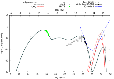
4.1.1 Mrk 421
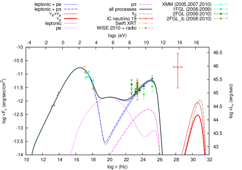
As already pointed out in the introduction, the most intriguing result of the leptohadronic modelling of Mrk 421 was the predicted muon neutrino flux, which was close to the IC-40 sensitivity limit calculated for the particular source by Tchernin et al. (2013). This is shown in Fig. 3 (left panel). We note that in the original paper DPM14, whose results we quote here, the Fermi/LAT data (Abdo et al., 2011) shown as grey open symbols in Fig. 3 were not included in the fit, since they were not simultaneous with the rest of the observations. The total and muon neutrino spectra are plotted with dotted and solid red lines, respectively. We use the same convention in all figures that follow, unless stated otherwise. The bump that appears two orders of magnitude below the peak of the neutrino spectrum in energy originates from neutron decay; we refer the reader to DPM14 for more details.
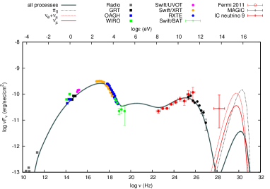
According to PR14, Mrk 421 is the most probable counterpart of the corresponding IceCube event (ID 9). This is now included in the right panel of Fig. 3, where the time-averaged SED during the MW campaign of January 2009 - June 2009 (Abdo et al., 2011) is also shown666All data points are taken from Fig. 4 in Abdo et al. (2011).. As we have already pointed out in Sect. 3, in order to avoid repetition, we did not attempt to fit the new data set of Abdo et al. (2011). Thus, the model photon (black line) and neutrino (red line) spectra depicted in the right panel of Fig. 3, were obtained for the same parameters used in DPM14 (see also Table 2), except for the Doppler factor, which was here chosen to be . The fit to the 2009 SED is surprisinly good, if we consider the fact that we used the same parameter set as in DPM14 with only a small modification in the value of the Doppler factor.
We note that the MW photon spectra shown in both panels have not been corrected for EBL absorption in order to demonstrate the relative peak energy and flux of the neutrino and components. The -ray emission from the decay is shown in both panels as a bump in the photon spectrum, peaking at Hz. Although the model prediction for the ratio of the -ray luminosity to the total neutrino luminosity is roughly two (see e.g. DMPR12), the component shown in Fig. 3 is suppressed because of internal photon-photon absorption. To demonstrate better the effect of the latter, we over-plotted the component that is obtained when photon-photon absorption is omitted (dash-dotted grey lines). In the figures that follow, we will display, for clarity reasons, the component only before its attenuation by the internal synchrotron and EBL photons.
Abdo et al. (2011), whose data we use here, have also presented a hadronic fit to the SED. Thus, a qualitative comparison between the two models is worthwhile. Both models are similar in that they require a compact emitting region and hard injection energy spectra of protons and primary electrons. Morevoer, the -ray emission from MeV to TeV energies, in both models, has a significant contribution from the hadronic component. However, the models differ in several aspects because of: (i) the differences in the adopted values for the magnetic field strength and maximum proton energy; (ii) the Bethe–Heitler process, which acts as an injection mechanism of relativistic pairs. Because of the strong magnetic field and large used in Abdo et al. (2011), the -ray emission from Mrk 421 is mainly explained as proton and muon synchrotron radiation. In our model, however, these contributions are not important, and the -rays in the Fermi/LAT and MAGIC energy ranges are explained mainly by synchrotron emission from pairs (see DPM14). Moreover, the emission from hard X-rays up to sub-MeV energies is attributed to different processes. In our model, it is the result of synchrotron emission from Bethe–Heitler pairs, whereas in the hadronic model of Abdo et al. (2011), this is explained as synchrotron emission from pion-induced cascades. It is important to note that the Bethe–Heitler process was not included in the hadronic model of Abdo et al. (2011).
As far as the neutrino emission is concerned, we find that the model-predicted neutrino flux is below but close to the 1 error bar of the derived value for the associated neutrino 9 (PR14). This proximity is noteworthy and suggests that the proposed leptohadronic model for Mrk 421 can be confirmed or disputed in the near future, as IceCube collects more data. Even in the case of a future rejection of the proposed model for Mrk 421, there will still be room for leptohadronic models that operate in a different regime of the parameter space. For example, in the LHs model, the neutrino spectrum is expected to peak at higher energies and to be less luminous than the one derived here, because of the higher values of and (see also in DPM14); this would also hold for the hadronic scenario used in Abdo et al. (2011), although no discussion of neutrinos is presented therein. For such leptohadronic variants, PeV neutrino observations cannot be model constraining.
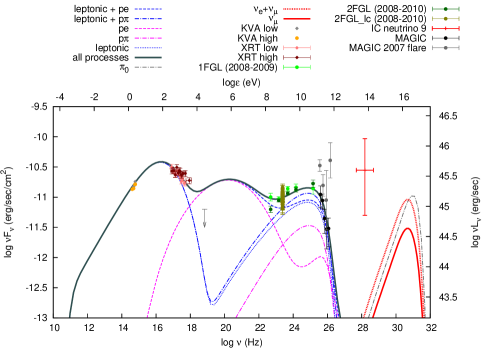
4.1.2 PG 1553+113
The hybrid SED of blazar PG 1553+113 is shown in Fig. 4. The contribution of different emission processes to the total SED is depicted with different types of lines, which are explained in the legend above the figure. The same applies to all figures that follow. We did not do the same for the case of Mrk 421, since we quoted results originally presented elsewhere, where a detailed description of the various processes contributing to the overall SED can be found. In any case, it was the prediction of the model about the neutrino flux from Mrk 421 we wanted to emphasize and not the spectral modelling of the SED. A few things about the hybrid SED are worth mentioning. It is the SSC emission of primary electrons (blue dotted line) that mainly contributes to the GeV-TeV -ray regime, whereas the component is hidden below it (magenta dash-dotted line). Notice also that the other component of photohadronic origin, namely the synchrotron emission from Bethe–Heitler pairs (magenta dashed line), has approximately the same peak flux as the component. The fact that the SSC emission is favoured with respect to the emission from photohadronic processes has to do with the particular choice of parameter values (Table 2). Besides the weak magnetic field ( G), the combination of a large source ( cm) and a relatively high Doppler factor (), decreases the compactness of the primary synchrotron photon field, which is the target for the photohadronic interactions, and eventually leads to a suppression of the proton cooling due to photohadronic processes and of the respective emission signatures (for more details, see Sect. 3.3 in PM15).
In our framework, the total neutrino luminosity is expected to be of the same order of magnitude as the synchrotron luminosity of pairs that is emitted as high-energy -rays (see also PM15). This is clearly shown in Fig. 4, where the peak luminosity of the component is similar to the one of the neutrino component (red dotted line). Taking into account that the component has a small contribution to the -ray emission, we expect also the peak neutrino flux to be lower than the peak -ray flux, which is verified numerically (see Fig. 4).
The previous results may be quantified through the ratio , which is defined as
| (13) |
where and are the total neutrino and TeV -ray luminosities, respectively, as measured in the observer’s frame. The ratio expresses the link between the observed -ray luminosity and the model-predicted neutrino luminosity from a blazar, and as such is as an important parameter of this study; this will become clear later in Sect. 4.3.
For PG 1553+113, in particular, we find , which suggests that the component is not the sole contributor to the observed -ray flux. Since the low value of is a matter of parameter values, it might make the reader wonder why we adopted the specific parameter values in the first place, and why we did not search for parameter sets that would favour photopion production. There are two profound reasons for our particular choice: the shape of the Fermi/LAT spectrum, and the hard X-ray observations with Swift/BAT. Although a higher proton injection luminosity or a more compact emitting region would lead to higher neutrino fluxes and could, thus, account for the neutrino event ID 17, it would inevitably raise the Bethe–Heitler component. Since the emission from pe pairs falls, in general, in the hard X-ray and soft gamma-ray energy bands, the Bethe–Heitler component would not only exceed the BAT observations but also destroy the fit to the low-energy Fermi/LAT data. One must also take into account that the synchrotron spectrum is broader around its peak than the SSC one, which would make it difficult to explain the observed Fermi/LAT spectrum.
Inspection of Table 2 reveals that PG 1553+113 is the second most energetically demanding case, with being approximately one order of magnitude higher than the other values. In terms of parameter values, such as the size and the magnetic field, it is an “outlier” of the sample. This should not come as a surprise, since PG 1553+113 is the most distant BL Lac of our sample with an estimated redshift (see Sect. 3), and its -ray flux is approximately equal to that of Mrk 421. PG 1553+113 is, therefore, an intrinsically more luminous source than Mrk 421 and requires an accordingly higher proton injection luminosity as measured in the comoving frame, unless a larger value for Doppler factor () was adopted. For a given this would lower the required proton compactness, and thus . We attempted, however, to avoid higher Doppler factors than those listed in Table 2, since those would shift the neutrino peak to hundreds of PeV in energy (see equation (4)).
Even for the adopted parameters, the peak energy of the model-derived neutrino spectrum is PeV. If we combine this with the hardness of the spectrum we obtain a much lower flux than the observed one, at the energy of the associated neutrino event; still, this lies within the 3 error bars (see also Sect. 4.2).
In Fig. 4 we have also included the X-ray high flux state of 2005 for illustrating reasons. An association of a higher X-ray flux with a higher neutrino flux would be intriguing, since it would bring the model-derived flux shown in Fig. 4 even closer to the observed one. However, such an association is not trivial in the absence of simultaneous observations in high-energies; neither GeV nor TeV data were available during the 2005 X-ray high state (see Fig. 1 in Aleksić et al. 2012). Consider for example a scenario where the increase in the X-ray flux is caused by an increase of the electron injection compactness. This would also result in a higher -ray flux, since the emission from both the SSC and components would increase. Finally, it would lead to a higher neutrino flux because of the higher synchrotron photon compactness. However, if the X-ray high flux state was not accompanied by an increase in the -ray emission, the aforementioned scenario would not be viable. More than one model parameters should be changed, and, depending on their combination, the derived neutrino flux would also differ. Because of the wide range of possibilities we do not, therefore, attempt to fit the high-state observed in the X-rays, nor to calculate the respective neutrino flux.
4.1.3 1ES 1011+496
The hybrid SED is shown in Fig. 5 and the resemblance to the model SED of PG 1553+113 is obvious. The -ray emission is mainly attributed to the SSC emission of primary electrons, since the flux of the component is only a small fraction of the observed -ray one. The fact that the model neutrino peak flux is lower than the peak -ray flux should come as no surprise after the discussion in Sect. 4.1.2. The model in Fig. 5 is mainly constrained by the simultaneous optical, soft X-ray and TeV data of the 2008 MW campaign, since there are no significant spectral variations in the Fermi/LAT observations covering the period 2008-2010. As already noted in PM15, any information on the hard X-ray emission, e.g. keV, would be even more constraining for the model. This becomes also evident from the cases of PG 1553+113 and H 2356-309 shown in Figs. 4 and 6, respectively.
We searched, therefore, a posteriori for possible detections or upper limits in the hard X-ray band, even if these were not, strictly speaking, simultaneous with the 2008 data. For this, we used the fourth INTEGRAL/IBIS catalog in 20-40 keV (Ubertini et al., 2009), that covers the period 2003-2008. The source has never been detected within this period, which resulted in the upper limit of erg cm-2 s-1 shown with a grey arrow in Fig. 5. The model SED exceeds by a factor of the upper limit. This suggests that the photohadronic emission (both pe and ) should decrease, if we were to include the upper limit into our fitting procedure. Since the most straightforward way to decrease the photohadronic emission in order to accommodate the hard X-ray constraint is to assume a lower , the derived value for listed in Table 2 should be considered only as upper limit. A lower (keeping all other parameters unaltered) would also result in an accordingly lower neutrino flux and, thus, lower . Given that the model neutrino flux at the same energy bin with neutrino event 9 is already below the observed one by approximately two orders of magnitude (see Figs. 5 and 10), we argue that the hard X-ray constraint makes the connection of 1ES 1011+496 with the neutrino event 9 even less plausible.
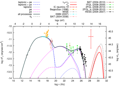
4.1.4 H 2356-309
H 2356-309 is one of the sources in the sample that has also been detected in TeV energies by H.E.S.S. and is the most probable counterpart for the IceCube neutrino with ID 10. Our model SED and neutrino flux are shown in Fig. 6. In contrast to PG 1553+113, the Fermi/LAT spectrum can be approximated as within the error bars and the -ray flux at TeV is order of magnitude below the peak flux of the low-energy hump. The properties of the observed SED of H 2356-309 allows us, therefore, to search for parameters that favour the emission and suppress the contribution of the SSC component, contrary to the cases of PG 1553+113 and 1ES 1011+496.
By adopting cm, which is smaller by two and one orders of magnitude than the source’s radius used for PG 1553+113 and 1ES 1011+496, respectively, we increase the photon compactness of the source. Moreover, the choice of a stronger magnetic field ( G) results in higher magnetic compactness () than before, where and is a measure of the synchrotron cooling rate. Thus, the synchrotron emission by secondary pairs from pe and processes is enhanced compared to the previous two cases. Figure 6 displays the above. It is, indeed, the emission from the pairs that mainly contributes to the observed -ray flux, while the SSC component is orders of magnitude less luminous. Moreover, the “Bethe–Heitler bump” becomes a prominent feature of the SED. Both results suggest a higher efficiency of both photohadronic processes compared to the previous two cases.
The neutrino spectral shape is similar to the previous cases and peaks at PeV. However, the ratio increases to , an eightfold increase from the case of PG 1553+113, which reflects the different efficiencies of photopion production in these cases. Although is close to unity, the peak neutrino peak flux is higher than the peak -ray flux because of the different spectral shapes of the two components. At the energy of the detected neutrino ( PeV) the model-derived flux is low, but lies within the 3 error bars. This discrepancy is similar to the one we found in previous cases, such as PG 1553+113, although the photopion production efficiency and are both higher in the case of H 2356-309. At first sight, this result seems contradictory. However, one has to take also into consideration the differences in the ratios of the observed -ray and neutrino fluxes. For example, in blazars PG 1553+113 and H 2356-309, this ratio is close to and much less than unity, respectively. Thus, in the case of H 2356-309, the higher is compensated by the lower ratio of observed -ray and neutrino luminosities.
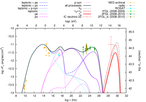
4.1.5 1H 1914-194
Blazar 1H 1914-194 is one of the two sources that are potential TeV emitters and has the poorest MW coverage among the BL Lacs of the sample (for details, see Sect. 3). Because of the inhomogeneity (in time domain) of the available MW observations, we present only an indicative fit, where we attempted to describe at best the Fermi/LAT data. Being the least constrained case we chose parameters that ensure high efficiency in photopion production, i.e. we present the most optimistic, for neutrino emission, scenario. We caution the reader that contemporaneous data in optical, X-rays and GeV -rays may strongly constrain the model (see e.g. Mrk 421 and PG 1553+113) and lead to different parameter values from those listed in Table 2. The neutrino flux shown in Fig. 7 should be therefore considered as an upper limit. We also note that the non-detection of TeV -rays is not as important for the predicted neutrino flux as the simultaneous coverage in the aforementioned energy bands. For example, the peak neutrino energy is solely determined by the peak frequency of the low energy component and the value of the Doppler factor (see equation (4)), while the neutrino flux is related to the sub-TeV -ray flux (see Figs. 4, 6 and Fig. 8 in PM15).
The SED we obtained is the most complex one in terms of the number of emission components that appear in the MW spectrum. Apart from the very low frequencies (below UV) where the primary leptonic component contributes, the spectrum is comprised roughly of: proton synchrotron radiation (between UV and keV), synchrotron emission from Bethe–Heitler pairs (between keV and 100 MeV) and synchrotron emission ( TeV) from secondary pairs produced through pion decay and absorption of VHE -rays (see equation (14) in Petropoulou & Mastichiadis 2012). In fact the role of absorption is non-negligible in this case, since the unattenuated component has a flux higher by a factor of than the neutrino one (see dash-dotted grey curve). The attenuation of VHE -rays initiates an EM cascade (Mannheim et al., 1991) that transfers energy from the PeV regime to lower energies. Our numerical approach does not allow us to isolate multiple photon generations produced in the electromagnetic cascade. Thus, strictly speaking, the pe and components shown in Fig. 7 are the result of synchrotron radiation not only from pairs produced through photohadronic interactions but also from pairs produced in the EM cascade.
In this case, we find , which is the highest value amongst the sample (see Table 2) and close to the maximum value () that is allowed in this theoretical framework (see Sect. 3.2 in PM15). The model-predicted neutrino flux is close to the observed flux (within the 1 error bars), thus strengthening the association of neutrino event 22 with this source. We have to note, however, that the model-predicted neutrino flux might decrease, should more constraints on the SED be available in the future.
4.1.6 1 RXS J054357.3-553206
1 RXS J054357.3-553206 is the second HBL source that has not yet been detected in TeV energies and the most probable counterpart of IceCube event 19 according to PR14. The hybrid SED obtained with our model is shown in Fig. 8 and shares many features with the model SED of PG 1553+113. According to the discussion in Sect. 4.1.2, we can infer that the observed -ray emission originates only partially from photohadronic processes, since the model derived neutrino peak flux is lower than the -ray one. In fact, we find that , same as in the case of PG 1553+113. However, because the flux corresponding to neutrino event ID 19 is higher than the -ray one, the model-predicted flux (at the same energy bin as event 19) is more than 3 off from the observed value, and the model prediction falls short of explaining the observed flux (see also Fig. 10).
In contrast to PG 1553+113 the SED of blazar 1 RXS J054357.3-553206 is less constrained both in (sub)MeV and TeV energies. This, along with the large discrepancy between the model and observed neutrino fluxes, makes 1 RXS J054357.3-553206 the best case for studying the effects of a different parameter set on the neutrino flux. We search, therefore, for parameters that increase the contribution of the component to the observed -ray emission and at the same time lead to a higher neutrino flux. We do not focus, however, on the goodness of the SED fit but we rather try to roughly describe the observed spectrum. The aim of what follows is (i) to demonstrate the flexibility of the leptohadronic model in describing the MW photon spectra and (ii) to find parameters that maximize the predicted neutrino flux from the particular blazar, albeit at the cost of a worse description of the SED.
Our results are summarized in Fig. 9, where we plot the hybrid SED obtained for a different parameter set presented in Table 3. From this point on, we will refer to it as Model 2. For a better comparison, we over-plotted with dashed lines the photon and neutrino spectra that were obtained for the parameters listed in Table 2 (Model 1). In Model 2 the -ray emission is mainly attributed to the component and the neutrino flux is comparable to the observed -ray one; in particular, we find . In our framework, this is the most optimistic scenario and the derived neutrino flux can be considered as an upper limit on the flux expected from this source (see also discussion in Sect. 4.1.5). However, the description of the SED is not as good as in our baseline model. In particular, the model-derived spectrum (i) cannot explain the highest energy Fermi/LAT data, (ii) is less hard (in units) at GeV energies and more broad than the observed one – see also Sect. 4.1.2, and (iii) is marginally above the highest flux observation in X-rays. This excess is caused by the synchrotron emission from Bethe–Heitler pairs, which appears in the hard X-ray/sub-MeV energy range, and it is even more luminous than the component. It is also noteworthy that the Bethe–Heitler emission in Model 2 plays a crucial role in the neutrino production: if we were to neglect pair injection from the Bethe–Heitler process, the neutrino flux in Model 2 would be lower by a factor of .
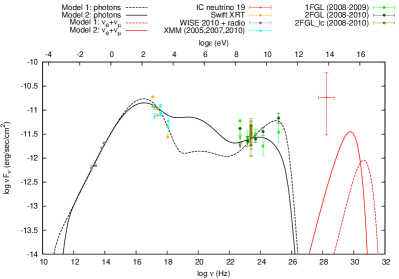
The detection of a luminous component in the 20 keV–20 MeV energy range could, therefore, serve as an indirect probe of high-energy neutrino emission from a blazar source within the leptohadronic scenario, as recently proposed in PM15.
4.2 Neutrino emission
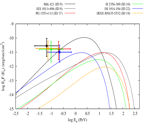
The model-derived electron and muon spectra for the six blazars of the sample are summarized in Fig. 10. For a better comparison, we over-plotted the fluxes that correspond to the respective neutrino events along with the Poissonian error bars calculated for a single event (PR14). We note that respective 3 error bars correspond to -2.9, +0.9 dex (Gehrels, 1986).
We focus first on the neutrino event 9, which according to the model-independent analysis of PR14, has two plausible astrophysical counterparts; namely blazars Mrk 421 and 1ES 1011+496. For Mrk 421, in particular, we show the neutrino spectrum depicted in the right panel of Fig. 3. According to the discussion in Sect. 5, the neutrino spectrum for 1ES 1011+496 (dashed line) should be considered as an upper limit, since inclusion of additional constraints in the SED fitting would lower the neutrino flux by at least a factor of . Thus, our results strongly favour Mrk 421 against 1ES 1011+496. As already discussed in the respective paragraphs of Sect. 4, the differences between the neutrino fluxes originate from the differences in their SEDs. Thus, the case of neutrino ID 9 reveals in the best way how detailed information from the photon emission may be used to lift possible degeneracies between multiple astrophysical counterparts.
1 RXS J054357.3-553206 was selected by PR14 as the astrophysical counterpart of neutrino event 19. Figure 10 shows the respective neutrino spectrum (yellow line) we obtained for the best-fit model of its SED. The model-derived flux at the energy of PeV lies below the 3 error bars. In this regard, 1 RXS J054357.3-553206 may be excluded at the present time from being the astrophysical counterpart of its associated neutrino event, namely event 19. We note, however, that a higher neutrino flux (within the 3 error bars) can be obtained at the cost of a worse description of the SED (see Sect. 8).
In all other cases, the model-derived777We refer to the neutrino emission calculated for best-fit SED models. neutrino flux at the energy bin of the detected neutrino is below the 1 error bars, but still within the 3 error bars. Thus, strictly speaking, the association of these sources cannot be excluded at the present time. In particular, Mrk 421 and 1H 1914-194 are the two cases with the smallest discrepancy between the observed and model-derived fluxes and, in this regard, the most interesting, because their association with the respective IceCube events can be either verified or disputed in the near future.
Besides the comparison between the model and the observed neutrino fluxes, Fig. 10 also demonstrates the similarity of the model neutrino spectra, despite the fact that they were obtained for BL Lacs with different properties. Our results suggest that the shape of the neutrino spectrum depends only weakly on the -ray luminosity of the source, which varies approximately two orders of magnitude among the members of the sample (see Table 2). In particular, the neutrino spectrum may be described as a power-law, i.e. with .
Before closing this section, we must point out that the present theoretical framework allows us to establish a connection between the observed -ray luminosity and the predicted total neutrino luminosity. In fact, we showed that these are simply proportional as , with in the range (Table 2). Although there is a maximum value predicted by the model, i.e. (see also PM15), there is no restriction on the lowest possible value of this ratio. Values of will only imply that the leptohadronic model simplifies into a pure leptonic one, with the SSC emission of primary electrons being responsible for the observed emission. This is illustrated best through the cases of PG 1553+113, 1ES 1011+496, and 1 RXS J054357.3-553206.
| Parameter | Model 1 | Model 2 |
|---|---|---|
| B | 0.1 | 1 |
| (cm) | ||
| 31 | 50 | |
| 1 | 1 | |
| 1.7 | 1.7 | |
| 1 | 1 | |
| 2.0 | 1.9 | |
| (erg/s) | ||
| (erg/s) | ||
| 0.1 | 3.1 |
4.3 The ratio and the energetics
In this section we examine in more detail the results presented in Table 2. We attempt to extract information about the dependence of the ratio , which is a crucial derivable quantity of our model, on observables, such as the photon index in the Fermi energy range and the -ray luminosity . Moreover, using the parameter values of Table 2, we calculate the jet power for each source and comment on the energetics. The results that follow, particularly those related to trends and correlations, should be considered with caution because of the limited size of the sample. Although these cannot be directly applied to a wider sample of BL Lacs, they are useful in that they provide a better understanding of the modelling results.
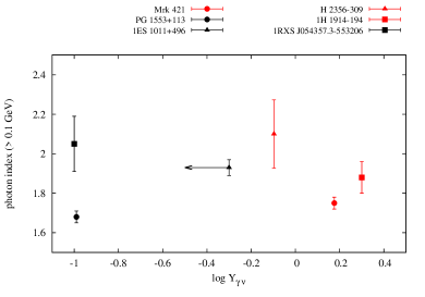
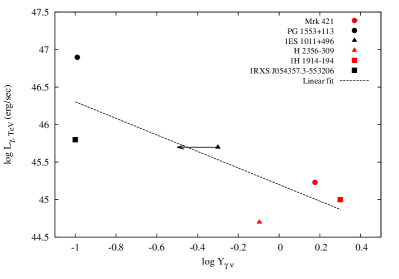
In the top panel of Fig. 11 we plot the photon index in the Fermi/LAT energy range (Abdo et al., 2010) versus the ratio . Sources with ratio values above and below the mean value of the sample are plotted with black and red symbols, respectively. We remind the reader that for 1ES 1011+496 the ratio was derived without including in our analysis the upper limit to the hard X-rays. As discussed in Sect. 5, inclusion of the hard X-ray constraint would lower the current ratio, at least by a factor of ; this is illustrated with an arrow in both panels of Fig. 11. There is no evident trend between the ratio and the photon index in the GeV energy range, although in Sect. 4.1.2 we used the hardness of the -ray spectrum as an argument for choosing parameters that favoured SSC against radiation. These findings suggest that the Fermi photon index alone is not a good indicator of the model-derived ratio . However, we find a negative trend between the observed -ray luminosity in the 0.01-1 TeV energy range (listed in Table 2) and the ratio (bottom panel in Fig. 11)888One could argue that we were bound to find an anti-correlation, since we are plotting against the ratio (note that ). This would be, indeed, correct, if there was an a priori knowledge of the model-derived neutrino luminosity. In fact, there was no guarantee that the neutrino luminosity obtained for all six BL Lacs would be approximately constant (see Table 2), which is an interesting outcome of the present analysis.. The size of our sample is limited, yet our results suggest that the contribution of the component to the blazar’s -ray emission is smaller in sources that are more -ray luminous. The dependence of on the -ray luminosity is particularly useful if we attempt to calculate the BL Lac diffuse neutrino flux by extrapolating the findings of this sample to the wider class of BL Lacs; this will be part of a future study. Finally, we point out that the negative trend shown in Fig. 11 does not necessarily mean that less powerful BL Lacs in -rays inject more power in relativistic protons, as it will become evident at the end of this section.
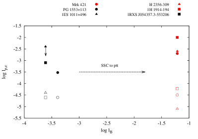
The bottom panel of Fig. 11 provides the first hints of a separation between the sources of the sample with ratios above and below the average value. However, this becomes clear in Fig. 12, where we plot the proton (filled symbols) and electron (open symbols) injection compactnesses against the magnetic compactness defined as . Red and black colored symbols are used to denote values of above and below the mean value, respectively. Figure 12 reveals the presence of two sub-groups within the sample. As increases, the synchrotron cooling of both primary and secondary electrons is enhanced. On the one hand, this leads to an increase of the synchrotron emission from pairs produced by interactions that emit in the -ray regime, while on the other hand, it suppresses the SSC emission of primary electrons. Thus, as increases, the contribution of the component to the -ray emission increases against the SSC one. This is finally reflected in an increase of the ratio .
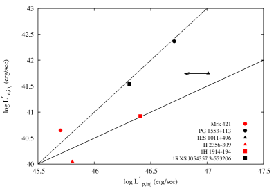
In Fig. 13 we plot as a function of . The color coding is the same as in Fig. 12 and the arrow stresses the fact that the derived value for 1ES 1011+496 is an upper limit (see Sect. 4.1.3). The injection luminosities of primary particles, as measured in the comoving frame, follow a more than linear relation, i.e. with . More important, though, is that sources with lie at the lower left corner of the plot, i.e. they are described by low proton and electron luminosities (in the comoving frame) with respect to the BL Lacs with smaller .
The jet power is a useful quantity when it comes to the energetics of the model. In the one-zone leptohadronic model, the energy densities of both relativistic electrons () and protons (), as well as the energy density of the magnetic field () and radiation (), contribute to the jet power, which may be written as
| (14) |
where the energy densities of the various components are measured at steady state and in the comoving frame, , and . For the assumptions used to derive equation (14), see e.g. Celotti & Ghisellini (2008). The jet luminosity as well as are listed, for reference, in Table 4. For all sources we find high jet luminosities, and emission regions far from equipartition , with the proton component being the dominant one. These results are typical of leptohadronic models (e.g. Böttcher et al. (2013); Cerruti et al. (2014)) and often constitute a point for criticism. However, our analysis highlighted that sources with , namely with significant contribution of the photohadronic component to the -ray emission, are described by less extreme, i.e. erg/s, jet powers and have lower ratios; this was not expected beforehand. For the rest of the sources, i.e. those with , the derived jet luminosities exceed erg/s, mainly because of the larger compared to the other sources (see Table 4).
| Source | (erg/s) | (erg/cm3) | (erg/cm3) | (erg/cm3) | (erg/cm3) |
|---|---|---|---|---|---|
| Mrk 421 | |||||
| PG 1553+113 | |||||
| 1ES 1011+496 | |||||
| H 2356-309 | |||||
| 1H 1914-194 | |||||
| 1 RXS J054357.3-553206 |
5 Discussion
In the present paper we have applied a one-zone leptohadronic model to six BL Lacs, which have been recently selected as the probable astrophysical counterparts (PR14) of five of the IceCube neutrino events (Aartsen et al., 2014), and calculated the neutrino flux in each case. In contrast to other studies, where the neutrino emission is calculated under the assumption of a generic blazar SED, here we obtained the neutrino signal from BL Lacs by fitting their individual SEDs. Thus, for each source, the photon and particle distributions used to derive the neutrino emission have to be determined individually, so as to give the observed SEDs.
For the SED modelling, we have adopted one of the possible leptohadronic model variants that allows us to directly associate the -ray blazar emission with a high-energy ( PeV) neutrino signal. In particular, the low-energy hump of the SED is explained by synchrotron radiation of primary relativistic electrons, whereas the observed high-energy (GeV-TeV) emission is the combined result of synchrotron self-Compton emission (from primary electrons) and of synchrotron radiation from secondary pairs. These are produced in a variety of ways, such as in Bethe–Heitler and pair production, and through the decays of charged pions, which themselves are the by-product of interactions of co-accelerated protons with the internally produced synchrotron photons. Secondary pairs produced in different processes have, in general, different energy distributions. Thus, in our framework, it is mainly the synchrotron emission of pairs that falls in the -ray regime, and in combination with the SSC radiation is used to explain the observed blazar emission in -rays.
BL Lacs are known for their variability across the electromagnetic spectrum and, because of this, we used SEDs that are comprised of nearly simultaneous MW observations. For those sources that were targets of recent MW observing campaigns we have adopted the data from the respective publications. In any other case, we have compiled the SEDs using the SED builder tool of the ASI Science Data Centre (ASDC). Only for one source in the sample (1H 1914-194), which had the poorest simultaneous MW coverage, had we to construct an SED using non-simultaneous data. We used the numerical code described in DMPR12 in order to calculate steady-state photon spectra that were later applied to the MW observations. Because of the multi-parameter nature of the problem (11-13 free parameters) and of the long numerical simulation time required for every parameter set, we have not performed a blind search of the available parameter space. To obtain a first estimate of the required parameter set, we used instead the analytical expressions presented in PM15. We then performed a series of numerical simulations using parameter values lying close to the initial parameter set, until a reasonably good fit to each SED was obtained.
Although the model-derived neutrino emission from the six BL Lacs that were selected as counterparts of the IceCube events was the main focus of this paper, our study highlighted also the flexibility of the leptohadronic model and its success in describing the blazar SEDs. This is particularly important, if one takes into account the following: (i) all sources in the sample were fitted using reasonable parameter values; (ii) these BL Lacs were not a priori selected for modelling purposes; and (iii) besides the fact that all sources in the sample were HBLs, they differed in many aspects, e.g. in redshift, in -ray luminosity and spectra.
The only source that may be excluded, at the present time, from being the astrophysical counterpart of the detected neutrino (event 19) is 1 RXS J054357.3-553206. In all other cases, the model-predicted neutrino flux is below the 1 but still within the 3 error bars of the respective IceCube neutrino events. In particular, for blazars Mrk 421 and 1H 1914-194 the model-derived neutrino fluxes at the same energy with the respective neutrino events (ID 9 and 22, respectively) were found to be very close to the low 1 error bars (Fig. 10). Although our results cannot be considered a proof of a firm association between these BL Lacs and the respective neutrinos, they can be verified or disputed in the near future, as IceCube collects more data and the observed fluxes become more constraining for the model.
Among the blazars of the sample, Mrk 421 is a special case. Its neutrino emission was calculated in a previous study (DPM14), at a time when there was no hint of a possible association between Mrk 421 and the IceCube events. DPM14 found that the neutrino flux from Mrk 421 was close to the current IceCube (IC-40) sensitivity limit for this source (left panel in Fig. 3). Of particular interest are the following:
-
•
the prediction of DPM14 was found a posteriori to be close to the observed flux related to neutrino ID 9;
- •
Apart from a direct comparison of the model and observed neutrino fluxes, we have shown that we can establish a direct connection between the observed -ray emission and the putative neutrino emission from a BL Lac source. We have quantified this relation by introducing the ratio of the total neutrino to the TeV luminosity (). In our model, for a given observed -ray luminosity that is purely explained by the synchrotron emission of pairs, i.e. when the SSC contribution is negligible, there is an upper limit to the neutrino luminosity. It can be shown that the limit is (see PM15). If, however, the SSC component is dominant in the -ray regime, we expect ; in this case, our model simplifies into a leptonic one. Thus, the spectrum of possible values is and corresponds to different contributions of the and SSC components to the -ray emission.
For the six blazars we have found ratios in the range , with a mean value . We have identified two sub-groups in the sample: blazars Mrk 421, H 2356-309 and 1H 1914-194 with and the rest with ratios below the average value (Table 2). Despite the small size of our sample, we have investigated the dependence of this ratio on observables of blazar emission. No hints of correlation with the photon index in the Fermi/LAT energy range were found (Fig. 11, top panel). However, we showed that there is a negative trend between and , i.e. more -ray luminous BL Lacs have a smaller photohadronic contribution to their -ray spectra (bottom panel in Fig. 11). Although this could be interpreted as a lower injection luminosity of relativistic protons, we showed that this is not the reason (see Fig. 13 and Table 4). Instead, the separation of sources according to can be understood in terms of the magnetic compactness. In Fig. 12 we demonstrated the transition from SSC to dominated -ray emission as the magnetic compactness gradually increases, which also translates to an increase of . Application of the model to a larger sample of BL Lacs is, however, necessary for a better understanding of the aforementioned trends.
Our analysis showed that the shape of the neutrino spectrum does not strongly depend on the -ray luminosity. In all cases, the neutrino spectra are described as with (Fig. 10). The peak energy of the neutrino spectrum, in the present context, depends only on one model parameter, namely the Doppler factor, and two observables, i.e. the peak frequency () of the low-energy hump of the SED and the redshift of the source . The dependence on the latter is not strong. Since all the sources of the sample are HBLs and we have obtained fits with similar values of , we should not expect large differences in the peak neutrino energy. We have verified this numerically, as demonstrated in Fig. 10. In addition to the similarity in the spectral shape, we have connected the expected neutrino luminosity from a BL Lac with its -ray luminosity in the 0.01-1 TeV energy range. Thus, one could go one step further and calculate the diffuse neutrino flux from BL Lacs, in order to see how it compares with the current IceCube detections and upper limits in the sub-EeV regime. Such a calculation requires an extrapolation of our findings to the wider class of BL Lacs, including low-synchrotron peaked blazars (LBLs), and the use of detailed simulations of the blazar population of the type done by Padovani & Giommi (2015). This will be the focus of a future study.
Similarly to other leptohadronic models, such as the proton synchrotron model (e.g. Böttcher et al. 2013), the derived jet power is high, ranging from erg/s up to a few erg/s, which implies a very low radiative efficiency. Moreover, the emitting region is far from equipartition, with the proton energy density being the dominant one – see Tables 4 in this work and Böttcher et al. (2013). The demanding energetics and the large departure from equipartition constitute the main point for criticism of our model, and of leptohadronic models in general. However, there are some important differences compared to the proton synchrotron model, which make this leptohadronic variant (LH) more flexible. On the one hand, strong magnetic fields ( G) are not necessary, while, on the other hand, proton acceleration to ultra-high energies () is not required. On the contrary, the upper cutoff of the proton distribution should be just a few times higher than (see equation (3)). In terms of the available parameter space of leptohadronic models, the LH variant occupies a sub-region, which corresponds, roughly speaking, to: low-to-moderate magnetic field strengths, moderate maximum proton energies, sub-pc sizes of the emission region ( cm) and high jet powers.
A detailed calculation of the neutrino emission from blazars following the so-called “blazar sequence” (Ghisellini et al., 1998) has been presented in two recent studies by Murase et al. (2014) and Dermer et al. (2014). Our analysis showed, however, that relatively high neutrino luminosities (of the order of erg/s) can be obtained from classical BL Lacs, with Mrk 421 being the most notable case. We note also that the production efficiency is low in all six blazars (see Table 2), and is in agreement with the expected values from BL Lacs (see equation (20) in Murase et al. 2014 and equation (28) in PM15). The question is then whether and how those results are compatible with each other. Figure 9 in Murase et al. (2014) shows that the typical neutrino luminosity of individual BL Lacs with no contamination by external photon fields (two lower blue curves) are erg/s, which is approximately 3 orders of magnitude below our typical values. The reason behind this discrepancy is the luminosity that is being injected into relativistic protons. In our analysis, we systematically used 2 to 3 orders of magnitude higher proton injection luminosities than Murase et al. (2014). This is mainly due to the fact that we try to model the observed blazar -ray emission in terms of photohadronic processes, whereas in Murase et al. (2014) and Dermer et al. (2014) it is not clear what the fate of the photons produced via photohadronic processes is, and why they do not appear in the observed SED. In any case, we compensate for the low number density of internal radiation by pushing the proton injection luminosity to higher values.
Another way to go around the problem of low photon number density in BL Lacs, which is related to low neutrino production efficiency, has been also recently presented in Tavecchio et al. (2014). Their approach is different than ours, though. In their model, BL Lacs can still be efficient neutrino emitters if the number density of photons, which are the targets for interactions, is enhanced. In order to achieve this, Tavecchio et al. (2014) assume a structured BL Lac jet with a fast spine and slow layer (Ghisellini et al., 2005; Tavecchio & Ghisellini, 2008), where the target field for interactions is the radiation field from the layer that appears boosted in the rest frame of the spine.
The recent correlation analysis of IceCube neutrino events and -ray sources by PR14 led to a somewhat unexpected result: instead of the more powerful FSRQs, it was BL Lacs that were among the most plausible astrophysical counterparts of 9 IceCube neutrinos. In general, FSRQs are expected to be efficient PeV neutrino emitters, because of their higher -ray luminosity, but more importantly, because of the dense external photon fields (broad line region and/or dusty torus). The absence of FSRQs from the list of probable astrophysical counterparts may be related to the “energetic criterion” applied by PR14. This was totally empirical and observationally driven, since it assumed only a tight photon – neutrino connection; any other more sophisticated choice of a diagnostic would be model-dependent. Thus, sources where a simple extrapolation of the -ray flux to the PeV energies lied much below the observed neutrino flux (taking into account the uncertainty in the flux measurement) were discarded. Relaxing this constraint would certainly increase the number of candidates, which might include FSRQs, but these would then depend on the specific model assumed.
In principle, the leptohadronic variant we presented here can also be applicable to FSRQs, with the appropriate choice of parameters. Because of the higher -ray luminosities and lower peak energies of FSRQs with respect to HBLs, a straightforward way to apply our model to FSRQs would be to increase the proton injection luminosity, while lowering the maximum proton energy. Taking into account the presence of additional photons originating from the broad line region and/or the torus, the model-predicted (PeV) neutrino luminosity would be much higher than the one derived for the HBLs in our sample and possibly close to, or at, the limit of flux detected by IceCube. The application of the model to the SEDs of FSRQs, however, may not be as simple as described above. Higher leads not only to increased emission from interactions but also from Bethe-Heitler interactions. Given its spectral shape and the typical energy range that emerges (see Figs. 3-9), it would be difficult to reconcile its emission with the flat X-ray spectra of FSRQs. However, more concrete answers can be given only with a detailed fitting of these type of sources.
6 Summary
Following the identification of eight BL Lac objects as likely sources of IceCube neutrinos by PR14, we set out to deduce the neutrino emission of the ones whose redshift is known by applying a leptohadronic model, using a variant of the model first discussed in Petropoulou & Mastichiadis (2012), albeit in a more general context. We used data from near simultaneous MW observations for all sources (as far as possible), and fitted the resulting SEDs in each individual case with steady-state photon spectra, which were obtained with the DMPR12 numerical code. Through the fitting procedure we determined the distributions of injected electrons and protons in what we assumed were spherical volumes of certain radii and magnetic field strengths, moving towards us with certain Lorentz factors; all the above being treated as free parameters.
Of the six BL Lacs with known redshift that we studied, one of them, Mrk 421, had been considered for its potential as a neutrino source in the past, by DPM14; the present study verifies that the neutrino event associated with it (ID 9) falls within its predicted flux. A good match between modeled and observed neutrino (ID 22) flux was also found for 1H 1914-194. 1 RXS J054357.3-553206, on the other hand, was the only BL lac to be confidently excluded as a source of its associated neutrino (ID 19), with the remaining three BL Lacs displaying some discrepancy between modeled and observed fluxes, but not enough to rule them out as sources at this stage. Depending on the shape of their SEDs, we found that some cases favour fits dominated by SSC while others favour fits dominated by photohadronic interactions, with the former having a lower ratio of neutrino to TeV -ray luminosities than the latter. This ratio, , which could prove important for calculations of the diffuse neutrino emission in the future, was then evaluated for its dependence on observable and model parameters. Ultimately, the results of our model should be confirmed or disproven in the near future, with the accumulation and data analysis of additional IceCube observations. Whatever the outcome, it will be important for constraining the available parameter space for leptohadronic models of blazar emission. This illustrates the importance of multi-messenger high-energy astronomy.
Acknowledgments
MP was supported by NASA through Einstein Postdoctoral Fellowship grant number PF3 140113 awarded by the Chandra X-ray Center, which is operated by the Smithsonian Astrophysical Observatory for NASA under contract NAS8-03060. ER acknowledges the support of the Deutsche Forschungsgemeinschaft (DFG)
References
- Aartsen et al. (2013) Aartsen M. G. et al., 2013, Physical Review D, 88, 112008
- Aartsen et al. (2014) Aartsen M. G. et al., 2014, Physical Review Letters, 113, 101101
- Abdo et al. (2010) Abdo A. A. et al., 2010, Astrophysical Journal Suppl. Ser., 188, 405
- Abdo et al. (2011) Abdo A. A. et al., 2011, Astrophysical Journal, 736, 131
- Aharonian et al. (2006a) Aharonian F. et al., 2006a, Astronomy & Astrophysics, 455, 461
- Aharonian et al. (2006b) Aharonian F. et al., 2006b, Astronomy & Astrophysics, 448, L19
- Aharonian (2000) Aharonian F. A., 2000, New Astron., 5, 377
- Ahlers & Murase (2014) Ahlers M., Murase K., 2014, Physical Review D, 90, 023010
- Albert et al. (2007a) Albert J. et al., 2007a, Astrophysical Journal Letters, 654, L119
- Albert et al. (2007b) Albert J. et al., 2007b, Astrophysical Journal Letters, 667, L21
- Aleksić et al. (2012) Aleksić J. et al., 2012, Astrophysical Journal, 748, 46
- Anderson & Filipovic (2009) Anderson M. W. B., Filipovic M. D., 2009, Serbian Astronomical Journal, 179, 7
- Asano & Mészáros (2014) Asano K., Mészáros P., 2014, Astrophysical Journal, 785, 54
- Atoyan & Dermer (2001) Atoyan A., Dermer C. D., 2001, Physical Review Letters, 87, 221102
- Atoyan & Dermer (2004) Atoyan A. M., Dermer C. D., 2004, NAR, 48, 381
- Baerwald et al. (2013) Baerwald P., Bustamante M., Winter W., 2013, ApJ, 768, 186
- Böttcher et al. (2013) Böttcher M., Reimer A., Sweeney K., Prakash A., 2013, Astrophysical Journal, 768, 54
- Carangelo et al. (2003) Carangelo N., Falomo R., Kotilainen J., Treves A., Ulrich M.-H., 2003, Astronomy & Astrophysics, 412, 651
- Celotti & Ghisellini (2008) Celotti A., Ghisellini G., 2008, Monthly Notices of the Royal Astronomical Society, 385, 283
- Cerruti et al. (2014) Cerruti M., Zech A., Boisson C., Inoue S., 2014, ArXiv e-prints
- Cherry et al. (2014) Cherry J. F., Friedland A., Shoemaker I. M., 2014, ArXiv e-prints
- Coppi & Aharonian (1999) Coppi P. S., Aharonian F. A., 1999, Astrophysical Journal Letters, 521, L33
- Dermer et al. (2014) Dermer C. D., Murase K., Inoue Y., 2014, ArXiv e-prints
- Dimitrakoudis et al. (2012) Dimitrakoudis S., Mastichiadis A., Protheroe R. J., Reimer A., 2012, Astronomy & Astrophysics, 546, A120
- Dimitrakoudis et al. (2014) Dimitrakoudis S., Petropoulou M., Mastichiadis A., 2014, Astroparticle Physics, 54, 61
- Esmaili et al. (2014) Esmaili A., Kang S. K., Dario Serpico P., 2014, ArXiv e-prints
- Falomo (1991) Falomo R., 1991, Astronomical Journal, 101, 821
- Fischer et al. (1998) Fischer J.-U., Hasinger G., Schwope A. D., Brunner H., Boller T., Trümper J., Voges W., Neizvestnyj S., 1998, Astronomische Nachrichten, 319, 347
- Forman et al. (1978) Forman W., Jones C., Cominsky L., Julien P., Murray S., Peters G., Tananbaum H., Giacconi R., 1978, Astrophysical Journal Suppl. Ser., 38, 357
- Fossati et al. (2008) Fossati G. et al., 2008, ApJ, 677, 906
- Franceschini et al. (2008) Franceschini A., Rodighiero G., Vaccari M., 2008, Astronomy & Astrophysics, 487, 837
- Gehrels (1986) Gehrels N., 1986, Astrophysical Journal, 303, 336
- Ghisellini et al. (1998) Ghisellini G., Celotti A., Fossati G., Maraschi L., Comastri A., 1998, Monthly Notices of the Royal Astronomical Society, 301, 451
- Ghisellini et al. (2005) Ghisellini G., Tavecchio F., Chiaberge M., 2005, Astronomy & Astrophysics, 432, 401
- Giovanoni & Kazanas (1990) Giovanoni P. M., Kazanas D., 1990, Nature, 345, 319
- Halzen & Zas (1997) Halzen F., Zas E., 1997, Astrophysical Journal, 488, 669
- H.E.S.S. Collaboration et al. (2010) H.E.S.S. Collaboration et al., 2010, Astronomy & Astrophysics, 516, A56
- Joshi et al. (2014) Joshi J. C., Winter W., Gupta N., 2014, Monthly Notices of the Royal Astronomical Society, 439, 3414
- Kirk & Mastichiadis (1989) Kirk J. G., Mastichiadis A., 1989, Astronomy & Astrophysics, 213, 75
- Kistler et al. (2013) Kistler M. D., Stanev T., Yuksel H., 2013, ArXiv e-prints
- Kneiske & Dole (2010) Kneiske T. M., Dole H., 2010, Astronomy & Astrophysics, 515, A19
- Krawczynski et al. (2002) Krawczynski H., Coppi P. S., Aharonian F., 2002, Monthly Notices of the Royal Astronomical Society, 336, 721
- Loeb & Waxman (2006) Loeb A., Waxman E., 2006, Journal of Cosmology and Astroparticle physics, 5, 3
- Mannheim (1995) Mannheim K., 1995, Astroparticle Physics, 3, 295
- Mannheim et al. (1991) Mannheim K., Biermann P. L., Kruells W. M., 1991, Astronomy & Astrophysics, 251, 723
- Mannheim et al. (2001) Mannheim K., Protheroe R. J., Rachen J. P., 2001, Physical Review D, 63, 023003
- Mastichiadis & Kirk (1997) Mastichiadis A., Kirk J. G., 1997, Astronomy & Astrophysics, 320, 19
- Mastichiadis et al. (2013) Mastichiadis A., Petropoulou M., Dimitrakoudis S., 2013, Monthly Notices of the Royal Astronomical Society, 434, 2684
- Mastichiadis et al. (2005) Mastichiadis A., Protheroe R. J., Kirk J. G., 2005, Astronomy & Astrophysics, 433, 765
- Mücke et al. (2000) Mücke A., Engel R., Rachen J. P., Protheroe R. J., Stanev T., 2000, Computer Physics Communications, 124, 290
- Mücke et al. (2003) Mücke A., Protheroe R. J., Engel R., Rachen J. P., Stanev T., 2003, Astroparticle Physics, 18, 593
- Mücke et al. (1999) Mücke A., Rachen J. P., Engel R., Protheroe R. J., Stanev T., 1999, Publications of the Astronomical Society of Australia, 16, 160
- Murase (2008) Murase K., 2008, PhysRevD, 78, 101302
- Murase et al. (2013) Murase K., Ahlers M., Lacki B. C., 2013, Physical Review D, 88, 121301
- Murase et al. (2014) Murase K., Inoue Y., Dermer C. D., 2014, ArXiv e-prints
- Nolan et al. (2012) Nolan P. L. et al., 2012, Astrophysical Journal Suppl. Ser., 199, 31
- Padovani & Giommi (2015) Padovani P., Giommi P., 2015, Monthly Notices of the Royal Astronomical Society, 446, L41
- Padovani & Resconi (2014) Padovani P., Resconi E., 2014, Monthly Notices of the Royal Astronomical Society, 443, 474
- Petropoulou (2014) Petropoulou M., 2014, Astronomy & Astrophysics, 571, A83
- Petropoulou et al. (2014) Petropoulou M., Giannios D., Dimitrakoudis S., 2014, Monthly Notices of the Royal Astronomical Society, 445, 570
- Petropoulou & Mastichiadis (2012) Petropoulou M., Mastichiadis A., 2012, Monthly Notices of the Royal Astronomical Society, 421, 2325
- Petropoulou & Mastichiadis (2015) Petropoulou M., Mastichiadis A., 2015, Monthly Notices of the Royal Astronomical Society, 447, 36
- Pita et al. (2014) Pita S. et al., 2014, Astronomy & Astrophysics, 565, A12
- Protheroe & Johnson (1996) Protheroe R. J., Johnson P. A., 1996, Astroparticle Physics, 4, 253
- Rachen & Mészáros (1998) Rachen J. P., Mészáros P., 1998, Physical Review D, 58, 123005
- Reinthal et al. (2012) Reinthal R. et al., 2012, Journal of Physics Conference Series, 355, 012017
- Reynoso (2014) Reynoso M. M., 2014, Astronomy & Astrophysics, 564, A74
- Sbarufatti et al. (2005) Sbarufatti B., Treves A., Falomo R., 2005, Astrophysical Journal, 635, 173
- Sikora et al. (2001) Sikora M., Błażejowski M., Begelman M. C., Moderski R., 2001, Astrophysical Journal, 554, 1
- Sikora et al. (1987) Sikora M., Kirk J. G., Begelman M. C., Schneider P., 1987, Astrophysical Journal Letters, 320, L81
- Stadnik & Romani (2014) Stadnik M., Romani R. W., 2014, Astrophysical Journal, 784, 151
- Stecker (1973) Stecker F. W., 1973, Astrophysics and Space Science, 20, 47
- Stecker et al. (1991) Stecker F. W., Done C., Salamon M. H., Sommers P., 1991, Physical Review Letters, 66, 2697
- Tavecchio & Ghisellini (2008) Tavecchio F., Ghisellini G., 2008, Monthly Notices of the Royal Astronomical Society, 385, L98
- Tavecchio et al. (2014) Tavecchio F., Ghisellini G., Guetta D., 2014, Astrophysical Journal Letters, 793, L18
- Tchernin et al. (2013) Tchernin C., Aguilar J. A., Neronov A., Montaruli T., 2013, ArXiv e-prints
- Ubertini et al. (2009) Ubertini P., Sguera V., Stephen J. B., Bassani L., Bazzano A., Bird A. J., 2009, Astrophysical Journal Letters, 706, L7
- Waxman & Bahcall (1997) Waxman E., Bahcall J., 1997, Physical Review Letters, 78, 2292
- Winter et al. (2014) Winter W., Becker Tjus J., Klein S. R., 2014, ArXiv e-prints
- Zhang & Kumar (2013) Zhang B., Kumar P., 2013, Physical Review Letters, 110, 121101