Comparison between exact and semilocal exchange potentials: An all-electron study for solids

Abstract

The exact-exchange (EXX) potential, which is obtained by solving the optimized-effective potential (OEP) equation, is compared to various approximate semilocal exchange potentials for a set of selected solids (C, Si, BN, MgO, Cu₂O, and NiO). This is done in the framework of the linearized augmented plane-wave method, which allows for a very accurate all-electron solution of electronic structure problems in solids. In order to assess the ability of the semilocal potentials to approximate the EXX-OEP, we considered the EXX total energy, electronic structure, electric-field gradient, and magnetic moment. An attempt to parameterize a semilocal exchange potential is also reported.

I Introduction

Given an expression for the total energy of an atom, molecule, or solid,

$$E_{\text{tot}}=T_{\text{s}}+E_{\text{en}}+E_{\text{H}}+E_{\text{xc}}+E_{\text{nn}},$$ (1)

where the terms on the right-hand side represent the noninteracting kinetic, electron-nucleus, Hartree, exchange-correlation, and nucleus-nucleus energies, respectively, the search for the Slater determinant which minimizes $E_{\text{tot}}$ leads to one-electron Schrödinger equations

$$\left(-\frac{1}{2}\nabla^{2}+v_{\text{en}}(\mathbf{r})+v_{\text{H}}(\mathbf{r})+\hat{v}_{\text{xc}}(\mathbf{r})\right)\psi_{i}(\mathbf{r})=\varepsilon_{i}\psi_{i}(\mathbf{r})$$ (2)

for the orbitals $\psi_{i}$ and their energies $\varepsilon_{i}$. [For ease of notation, all formulas are given in spin-unpolarized form and for non-zero gap systems. $N$ will denote the number of (doubly) occupied orbitals.] In the Kohn-Sham (KS)Kohn and Sham (1965) version of density functional theory (DFT),Hohenberg and Kohn (1964) the exchange-correlation potential $\hat{v}_{\text{xc}}$ is calculated as the functional derivative of $E_{\text{xc}}$ with respect to the electron density $\rho$ ($\hat{v}_{\text{xc}}=\delta E_{\text{xc}}/\delta\rho$) and, as a consequence, $\hat{v}_{\text{xc}}$ is a multiplicative potential ($\hat{v}_{\text{xc}}\psi_{i}=v_{\text{xc}}\psi_{i}$), i.e., it is the same for all orbitals. Instead, in the generalized KS (gKS) framework, formally introduced in Ref. Seidl et al., 1996, the derivative of $E_{\text{xc}}$ is taken with respect to $\psi_{i}$ ($\hat{v}_{\text{xc}}\psi_{i}=\delta E_{\text{xc}}/\delta\psi_{i}^{*}$) as in the Hartree-Fock (HF) method. In other words, in the KS method the minimization of the total energy [Eq. (1)] is done with the constraint that the orbitals forming the (single) Slater determinant are solutions to a Schrödinger equation with a multiplicative potential, whereas in the gKS scheme this constraint is dropped. For exchange-correlation functionals $E_{\text{xc}}$ which depend explicitly only on $\rho$ (and eventually its derivatives) like in the local density approximation (LDA) Kohn and Sham (1965) or generalized gradient approximation (GGA),Becke (1988); Perdew et al. (1996) the gKS method leads to the same multiplicative potential $v_{\text{xc}}$ as the KS method. However, for an orbital-dependent functional $E_{\text{xc}}$, i.e., a functional which depends on the orbitals $\psi_{i}$ not only via $\rho$, such as meta-GGA (see Ref. Sun et al., 2011 and references therein), self-interaction corrected,Perdew and Zunger (1981) or hybridBecke (1993) functionals, the gKS method leads to a non-multiplicative (i.e., orbital-dependent) potential $\hat{v}_{\text{xc}}=v_{\text{xc},i}$ as in the HF method. For such functionals, the calculation of $\delta E_{\text{xc}}/\delta\rho$, as required in the KS formalism, is highly non-trivial, but possible by solving the optimized effective potential (OEP) equation.Sharp and Horton (1953)

The focus of the present work will be on the multiplicative exchange potential $v_{\text{x}}$. More specifically, approximate semilocal exchange potentials will be compared to the exact exchange (EXX) potential obtained by means of the OEP method (called EXX-OEP thereafter), which has been implemented very recently Betzinger et al. (2011, 2012, 2013) within the linearized augmented plane-waveAndersen (1975); Singh and Nordström (2006); Blügel and Bihlmayer (2006) (LAPW) method for solids.

The advantage of semilocal potentials, which depend on the local quantities $\rho$, $\nabla\rho$, $\nabla^{2}\rho$, or the kinetic-energy density $t=\sum_{i=1}^{N}\nabla\psi_{i}^{*}\cdot\nabla\psi_{i}$ is that they are rather simple to implement and lead to calculations which are much faster than EXX-OEP calculations or HF/hybrid calculations with a non-multiplicative potential. The LDA exchange potential is for example a simple function of $\rho$, whereas in the case of GGA functionals, the corresponding potential becomes a function of $\rho$ and its first two derivatives.

The problem with the LDA and vast majority of GGA exchange functionals $E_{\text{x}}$ is that their functional derivative $v_{\text{x}}$ barely resembles the EXX-OEP potential.Engel and Vosko (1993a, b) Therefore several studies have focused on the search for better semilocal approximations for $v_{\text{x}}$ rather than $E_{\text{x}}$. Among these studies there are the early works of Engel and Vosko,Engel and Vosko (1993b) Baerends and co-workers, van Leeuwen and Baerends (1994); Gritsenko et al. (1995, 1996); Schipper et al. (2000) and the more recent works of Becke and Johnson,Becke and Johnson (2006) Staroverov and co-workers, Staroverov (2008); Gaiduk and Staroverov (2011, 2012); Gaiduk et al. (2015) Armiento et al., Armiento et al. (2008); Armiento and Kümmel (2013) and others.Umezawa (2006); Kuisma et al. (2010)

It is worth mentioning that all these approximations for $v_{\text{x}}$ can be categorized in one of these two groups, namely, those which are functional derivative of a functional $E_{\text{x}}$ and those which are not (such potentials were termed stray in Ref. Gaiduk et al., 2009). Examples of exchange potentials which were modelled with the constrained to be a functional derivative are the ones from Engel and VoskoEngel and Vosko (1993b) (EV93) and Armiento and Kümmel Armiento and Kümmel (2013) (AK13), while the potentials from van Leeuwen and Baerendsvan Leeuwen and Baerends (1994) (LB94) and Becke and JohnsonBecke and Johnson (2006) (BJ) are stray potentials. Not constraining a potential to be a functional derivative means much more freedom for its analytical form, however it has been shown that stray potentials have undesirable features both at the fundamental and practical level. Gaiduk and Staroverov (2009); Gaiduk et al. (2009); Karolewski et al. (2013) Furthermore, attempts to turn a stray potential into a functional derivative without loosing too much of its original features have been rather unsuccessful up to now (see Refs. Gaiduk and Staroverov, 2011, 2012; Karolewski et al., 2013).

As already mentioned above, various semilocal exchange potentials $v_{\text{x}}$ will be studied and compared to the EXX-OEP which will serve as reference. We will focus in particular on the BJ potential, which has been shown to reproduce quite well the EXX-OEP potential in atomsBecke and Johnson (2006); Staroverov (2008) and has been applied to molecules Gaiduk and Staroverov (2008); Oliveira et al. (2010) and solids,Tran et al. (2007) as well as modified to improve the results in various cases. Armiento et al. (2008); Staroverov (2008); Karolewski et al. (2009); Tran and Blaha (2009); Räsänen et al. (2010); Pittalis et al. (2010); Cerqueira et al. (2014) Furthermore, in an attempt to be as close as possible to the EXX-OEP potential, a more general form of the BJ potential will be proposed.

The paper is organized as follows. Section II gives a summary of the EXX-OEP method and introduces the tested semilocal exchange potentials, while the computational details are given in Sec. III. Then, the results are presented and discussed in Sec. IV. Finally, Sec. V gives the summary and an outlook for possible improvements.

II Theory

II.1 Optimized effective potential

As mentioned in the Introduction, the calculation of the multiplicative exchange-correlation potential $v_{\text{xc}}=\delta E_{\text{xc}}/\delta\rho$ for any orbital-dependent functional $E_{\text{xc}}$ can be achieved by solving the integro-differential OEP equationSharp and Horton (1953) for $v_{\text{xc}}$ (see Ref. Kümmel and Kronik, 2008 for a review), which is given in general by

$$\int\chi(\mathbf{r},\mathbf{r}^{\prime})v_{\text{xc}}(\mathbf{r}^{\prime})d^{3}r^{\prime}=\Lambda_{\text{xc}}(\mathbf{r}),$$ (3)

with

$$\Lambda_{\text{xc}}(\mathbf{r}) = \sum_{i}\left[\int\left(\frac{\delta E_{\text{xc}}}{\delta\psi_{i}(\mathbf{r}^{\prime})}\frac{\delta\psi_{i}(\mathbf{r}^{\prime})}{\delta v_{\text{eff}}(\mathbf{r})}+\text{c.c.}\right)d^{3}r^{\prime}\right.$$ (4)

$$\left.+\frac{\delta E_{\text{xc}}}{\delta\varepsilon_{i}}\frac{\delta\varepsilon_{i}}{\delta v_{\text{eff}}(\mathbf{r})}\right],$$

where $v_{\text{eff}}=v_{\text{en}}+v_{\text{H}}+v_{\text{xc}}$ is the KS effective potential and

$$\chi(\mathbf{r},\mathbf{r}^{\prime}) = \frac{\delta\rho(\mathbf{r})}{\delta v_{\text{eff}}(\mathbf{r}^{\prime})}$$ (5)

$$= 2\sum_{i=1}^{N}\sum_{j=N+1}^{\infty}\frac{\psi_{i}^{*}(\mathbf{r})\psi_{j}(\mathbf{r})\psi_{j}^{*}(\mathbf{r}^{\prime})\psi_{i}(\mathbf{r}^{\prime})}{\varepsilon_{i}-\varepsilon_{j}}+\text{c.c.}$$

is the KS (non-interacting) density response function.

So far, the OEP method has been applied mostly to the EXX energy

$$E_{\text{x}}^{\text{EXX}}=-\sum_{i=1}^{N}\sum_{j=1}^{N}\int\int\frac{\psi_{i}^{*}(\mathbf{r})\psi_{j}(\mathbf{r})\psi_{j}^{*}(\mathbf{r}^{\prime})\psi_{i}(\mathbf{r}^{\prime})}{\left|\mathbf{r}-\mathbf{r}^{\prime}\right|}d^{3}rd^{3}r^{\prime},$$ (6)

which has the same analytic form as the HF exchange energy, but is evaluated with the KS orbitals instead of the HF orbitals. In the case of EXX, the sum over $i$ in Eq. (4) runs over the occupied orbitals only [Eq. (6) does not depend on unoccupied orbitals] and $\delta E_{\text{xc}}/\delta\varepsilon_{i}=0$.

Talman and ShadwickTalman and Shadwick (1976) were the first who reported EXX-OEP calculations (on spherical atoms). Initially, EXX-OEP was proposed as an approximation to HF in order to get rid of the non-multiplicative HF potential. Later, it was recognized that the EXX-OEP method represents also the exact exchange method within the KS DFT framework (see, e.g., Ref. Engel and Vosko, 1993a and references therein). Since then EXX-OEP has attracted more and more attention. For solids the first EXX-OEP implementation was reported by Kotani.Kotani (1994) Subsequent reports of OEP calculations on solids (the focus of the present work) can be found in Refs. Kotani, 1995; Kotani and Akai, 1996; Kotani, 1998; Kotani and Akai, 1998; Städele et al., 1997, 1999; Aulbur et al., 2000; Fleszar, 2001; Magyar et al., 2004; Rinke et al., 2005; Qteish et al., 2005, 2006; Rinke et al., 2006; Grüning et al., 2006, 2006; Engel and Schmid, 2009; Betzinger et al., 2011, 2012, 2013; Klimes and Kresse, 2014.

The implementation of the OEP equation is rather complicated and its solution prone to instabilities in particular if localized basis functions are used.Staroverov et al. (2006); Görling et al. (2008); Gidopoulos and Lathiotakis (2012) Recently, the implementation of the EXX-OEP method within the LAPW method has been reported.Betzinger et al. (2011, 2012, 2013); Friedrich et al. (2013) It employs an auxiliary basis, the mixed product basis, for representing the OEP. As discussed in detail in Refs. Betzinger et al., 2011; Friedrich et al., 2013, in order to obtain a stable and physical EXX-OEP potential, the orbital (LAPW) and auxiliary (mixed product) basis sets have to satisfy a basis-set balance condition. This condition is fulfilled when the orbital basis set is converged with respect to the auxilary basis set and usually demands large orbital basis sets. The usage of (uneconomically) large LAPW basis sets can be avoided if the response of the LAPW basis functions is explicitly taken into account in the calculation of the KS orbital response $\delta\psi_{i}/\delta v_{\text{eff}}$ in Eq. (4) and the calculation of the KS density response [Eq. (5)]. Betzinger et al. (2012, 2013) In this way, a much faster convergence is achieved with respect to basis set size (and number of unoccupied states) and the basis balance condition is fulfilled with smaller orbital basis sets.

II.2 Semilocal potentials

Among the considered semilocal exchange potentials, LDA Kohn and Sham (1965) as well as the GGAs B88, Becke (1988) PBE,Perdew et al. (1996) EV93,Engel and Vosko (1993b) and AK13Armiento and Kümmel (2013) are functional derivatives of exchange-energy functionals that have the generic form

$$E_{\text{x}}=-\frac{3}{4}\left(\frac{3}{\pi}\right)^{1/3}\int\rho^{4/3}(\mathbf{r})F_{\text{x}}\left(s(\mathbf{r})\right)d^{3}r,$$ (7)

where $F_{\text{x}}\left(s\right)$ is the so-called exchange enhancement factor which depends on the reduced density gradient $s=\left|\nabla\rho\right|/\left(2\left(3\pi^{2}\right)^{1/3}\rho^{4/3}\right)$. LDA is the exact form for the homogeneous electron gas and corresponds to $F_{\text{x}}(s)=1$. As shown in Fig. 1, the enhancement factors of the GGA functionals are larger than one, thus correcting the tendency of LDA to underestimate the magnitude of the exchange energy. Compared to the standard PBE functional, EV93 and AK13 are much stronger. Note that at $s=0$ all factors $F_{\text{x}}(s)$ reduce to one in order to satisfy the homogeneous electron gas limit given by LDA. B88 and PBE, which are among the most popular GGA functionals for calculating the properties of molecules and solids, respectively, were constructed without considering the quality of the potential $v_{\text{x}}$. For EV93 and AK13, however, the emphasis was put on $v_{\text{x}}$. The parameters in EV93 were determined by a fit to EXX-OEP potentials in atoms,Engel and Vosko (1993b) while Armiento and Kümmel were able to find an analytical form for AK13 such that $v_{\text{x}}$ changes discontinuously at integer particle numbers.Armiento and Kümmel (2013) Both EV93 and AK13 were shown to improve over the standard LDA and PBE functionals for the band gaps in solids. Dufek et al. (1994); Tran et al. (2007); Armiento and Kümmel (2013); Vlček et al. (2015)

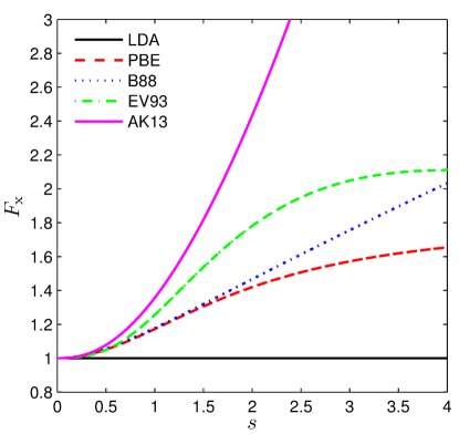
Figure 1: (Color online) The enhancement factors $F_{\text{x}}(s)$ [see Eq. (7)] of the different exchange functionals considered in this work.

In addition to these potentials, we consider in this work the BJ potentialBecke and Johnson (2006) which is of stray type (see Refs. Karolewski et al., 2009; Gaiduk and Staroverov, 2009) and has the form

$$v_{\text{x}}^{\text{BJ}}(\mathbf{r})=v_{\text{x}}^{\text{S/BR}}(\mathbf{r})+\frac{1}{\pi}\sqrt{\frac{5}{6}}\sqrt{\frac{t(\mathbf{r})}{\rho(\mathbf{r})}},$$ (8)

where $v_{\text{x}}^{\text{S/BR}}$ is either the Slater (S) potential Slater (1951)

$$v_{\text{x}}^{\text{S}}(\mathbf{r})=-\frac{2}{\rho(\mathbf{r})}\sum_{i=1}^{N}\sum_{j=1}^{N}\psi_{i}^{*}(\mathbf{r})\psi_{j}(\mathbf{r})\int\frac{\psi_{j}^{*}(\mathbf{r}^{\prime})\psi_{i}(\mathbf{r}^{\prime})}{\left|\mathbf{r}-\mathbf{r}^{\prime}\right|}d^{3}r^{\prime}$$ (9)

or the Becke-Roussel potentialBecke and Roussel (1989)

$$v_{\text{x}}^{\text{BR}}(\mathbf{r})=-\frac{1}{b(\mathbf{r})}\left(1-e^{-x(\mathbf{r})}-\frac{1}{2}x(\mathbf{r})e^{-x(\mathbf{r})}\right).$$ (10)

The function $x$ in Eq. (10) is calculated by solving (at each point of space) the nonlinear equation (or using the analytical interpolation formula for $x$ from Ref. Proynov et al., 2008)

$$\frac{x(\mathbf{r})e^{-2x(\mathbf{r})/3}}{x(\mathbf{r})-2}=\frac{1}{3}\left(\frac{\pi}{2}\right)^{2/3}\frac{\rho^{5/3}(\mathbf{r})}{Q(\mathbf{r})},$$ (11)

where

$$Q(\mathbf{r})=\frac{1}{12}\left(\nabla^{2}\rho(\mathbf{r})-4\gamma D(\mathbf{r})\right)$$ (12)

with

$$D(\mathbf{r})=t(\mathbf{r})-\frac{1}{8}\frac{\left|\nabla\rho(\mathbf{r})\right|^{2}}{\rho(\mathbf{r})}.$$ (13)

After $x$ is calculated, $b$ in Eq. (10) is given by

$$b(\mathbf{r})=\left(\frac{x^{3}(\mathbf{r})e^{-x(\mathbf{r})}}{4\pi\rho(\mathbf{r})}\right)^{1/3}.$$ (14)

The parameter $\gamma$ in Eq. (12) has to be set to 1 or 0.8 in order to recover the exact exchange potential of the hydrogen atom or the homogeneous electron gas, respectively.Becke and Roussel (1989) Note that since the BR potential and the second term of Eq. (8) depend on the kinetic-energy density $t$, they are of the semilocal meta-GGA form,Perdew et al. (2005) while the Slater potential [Eq. (9)] is nonlocal in the sense that the calculation of $v_{\text{x}}^{\text{S}}$ at $\mathbf{r}$ requires the value of quantities (the occupied orbitals) at all points of space $\mathbf{r}^{\prime}$. For closed-shell atoms it was shown that the BR potential is very close to the Slater potential.Becke and Roussel (1989); Becke and Johnson (2006) In the rest of this work, we focus on the BJ-based potentials using the BR potential.

Several modifications of the BJ potential have been proposed. Armiento et al. (2008); Staroverov (2008); Tran and Blaha (2009); Räsänen et al. (2010) For instance, in Ref. Tran and Blaha, 2009 we proposed the modified BJ (mBJ) potential

$$v_{\text{x}}^{\text{mBJ}}(\mathbf{r})=cv_{\text{x}}^{\text{BR}}(\mathbf{r})+\left(3c-2\right)\frac{1}{\pi}\sqrt{\frac{5}{6}}\sqrt{\frac{t(\mathbf{r})}{\rho(\mathbf{r})}},$$ (15)

where $c$ is a parameter that was introduced to improve the agreement with experiment for the band gaps in solids and that was parameterized using the average of $\left|\nabla\rho\right|/\rho$ in the unit cell.

As pointed out by Räsänen et al. in Ref. Räsänen et al., 2010, the BJ potential is not gauge-invariant, does not show the correct asymptotic behavior at $\mathbf{r}\rightarrow\infty$ in finite systems, and the correction to the Slater (or BR) term is not zero for one-electron systems as it should be. In order to cure these deficiencies, they proposed an universal correction (UC) to the BJ potential. For systems with zero current density $\mathbf{J}$ (like those considered in this work), the UC consists of replacing $t$ by $D$ [Eq. (13)] in the second term of Eq. (8).

In an attempt to propose in the present work a semilocal exchange potential which can reproduce accurately the EXX-OEP, we will consider a more general form of the BJ and mBJ potentials, called generalized BJ (gBJ) thereafter:

$$v_{\text{x}}^{\text{gBJ}}(\mathbf{r})=cv_{\text{x}}^{\text{BR}}(\mathbf{r})+\left(3c-2\right)\frac{\frac{1}{2}\left(\frac{3}{\pi}\right)^{1/3}}{\left(\frac{3}{10}\left(3\pi^{2}\right)^{2/3}\right)^{p}}\frac{t^{p}(\mathbf{r})}{\rho^{\left(5p-1\right)/3}(\mathbf{r})},$$ (16)

which, in addition to the two parameters $\gamma$ [in $v_{\text{x}}^{\text{BR}}$, Eq. (12)] and $c$ as in mBJ, contains a third one ($p$) whose value is $0.5$ in BJ and mBJ. The form of the second term of Eq. (16) was chosen such that the LDA exchange potential is recovered for constant electron densities (and if $\gamma=0.8$, see above). As a modification of Eq. (16), we will also consider its variant where $t$ in the second term is replaced by $D$ (UC, Ref. Räsänen et al., 2010), leading to the gBJUC potential. The parameters $\gamma$, $c$, and $p$ of the gBJ and gBJUC potentials were varied around the standard BJ values within the intervals $\left[0.4,1.4\right]$, $\left[1.0,1.4\right]$, and $\left[0.35,0.65\right]$ and in steps of $0.2$, $0.1$, and $0.05$, respectively. In the following, BJ will denote the unmodified potential given by Eq. (8) using BR with $\gamma=0.8$ and similarly for BJUC. The values of the parameters in the gBJ and gBJUC potentials will be specified in this order: $(\gamma,c,p)$.

\begin{picture}(8.0,17.0)(0.0,0.0)\put(0.0,11.2){\epsfbox{fig_1D_C_vx_gamma.pdf}} \put(0.0,5.6){\epsfbox{fig_1D_C_vx_c.pdf}} \put(0.0,0.0){\epsfbox{fig_1D_C_vx_p.pdf}} \end{picture}

Figure 2: (Color online) gBJ$(\gamma,c,p)$ exchange potentials in C plotted starting at a distance of 0.2 Å from the atom at site $(1/4,1/4,1/4)$ in the [111] direction. The center of the unit cell is at $d=2.32$ Å. The potentials were shifted such that $\int_{\text{cell}}v_{\text{x}}(\mathbf{r})d^{3}r=0$.

\begin{picture}(8.0,11.3)(0.0,0.0)\put(0.0,5.6){\epsfbox{fig_1D_C_vx_BJ_BJUC.pdf}} \put(0.0,0.0){\epsfbox{fig_1D_C_t_D.pdf}} \end{picture}

Figure 3: (Color online) (a) BJ and BJUC exchange potentials in C. (b) Ratio $t/D$ for C. The path and potential shift are as in Fig. 1.

Regarding the influence of the parameters $\gamma$, $c$, and $p$ on the shape of the gBJ potential, we have generally observed that an increase of one or another of the parameters leads to more pronounced variations, and this effect is rather similar for the three parameters (see Fig. 2 for an illustrative example in the diamond phase of C). Nevertheless, by looking more closely at Fig. 2, we can notice some differences in the way the parameters $\gamma$, $c$, and $p$ modify the potential. For instance, when $\gamma$ is increased [Fig. 2(a)], the intershell peak at $d\sim 0.4$ Å gets more spiky, while the value of $c$ affects the potential in a broader region of space [Fig. 2(b)]. This is the reason why we have found it useful to use three parameters instead of only one or two in our attempt for reproducing at best the EXX-OEP results with the gBJ(UC) potential.

The effect of the UC is shown in Fig. 3(a) by comparing the BJ and BJUC potentials in C. Rather large differences between the two potentials are visible in the core region ($d<0.4$ Å in this example) where the BJUC potential is much more attractive than BJ. As a consequence, the core states are bound stronger when the UC is used. We made the same observation for all other investigated solids (see also Fig. 3 of Ref. Räsänen et al., 2010 for the Ne atom). In Fig. 3(b), the kinetic-energy density $t$ and $D$ [Eq. (13)] are compared by showing the ratio $t/D$, where we can see that it is indeed in the core region that $t/D$ differs the most from 1. Actually, the term $\left|\nabla\rho\right|^{2}/\left(8\rho\right)$ in $D$ is the von Weizsäckerv. Weizsäcker (1935) kinetic-energy density which is equal to the exact kinetic-energy density $t$ in regions of space dominated by a single orbital. Therefore, in such regions $D=0$ and the BJUC potential reduces to the BR (or Slater) potential which is by far too negative compared to EXX-OEP.Becke and Johnson (2006) Note that the (smaller) differences between $t$ and $D$ in the region 0.4$-$1.4 Å also affect the potentials, however, due to the alignment of the different potentials $\left(\int_{\text{cell}}v_{\text{x}}(\mathbf{r})d^{3}r=0\right)$, the differences between BJ and BJUC are transferred to $d>1.2$ Å.

III Computational details

The calculations with the semilocal potentials and EXX-OEP were done with the WIEN2kBlaha et al. (2001) and FLEURFLE codes, respectively. Since the two codes use the same basis set (LAPWAndersen (1975); Singh and Nordström (2006); Blügel and Bihlmayer (2006)), it was also possible to calculate the EXX-OEP orbitals with WIEN2k by fixing the potential $v_{\text{x}}$ to the EXX-OEP read from a file (containing the radial functions and Fourier coefficients of the spherical harmonics and plane-wave expansions of the potential) generated by FLEUR. Despite some (small) technical differences between the two codes and different computational parameters used for the calculations (e.g., basis sets), we observed for all solids, that running a PBE calculation with WIEN2k as usual or with the FLEUR-generated PBE potential leads to very close results (e.g., the transition energies differ by less than 0.02 eV). Therefore, we are convinced that this procedure of calculating orbitals using a potential generated from another code is reliable in terms of accuracy. In addition, HF calculations with the WIEN2k code were also done. Note, however, that in the current implementation of the HF method,Tran and Blaha (2011) the core electrons experience a semilocal potential, like in other implementations of the HF method with the LAPW basis set.Massidda et al. (1993); Betzinger et al. (2010) The $\mathbf{k}$-mesh for the integration of the Brillouin zone and size of the basis sets were chosen to be converged for the purpose of our work.

The set of solids that we will consider consists of the nonmagnetic cubic (the space group, number of atoms in the primitive unit cell, and cubic lattice constant are indicated in parenthesis) C ($Fd\overline{3}m$, two atoms, 3.57 Å), Si ($Fd\overline{3}m$, two atoms, 5.43 Å), MgO ($Fm\overline{3}m$, two atoms, 4.23 Å), BN ($F\overline{4}3m$, two atoms, 3.62 Å), and Cu₂O ($Pn\overline{3}m$, six atoms, 4.27 Å). C, Si, and BN are covalent, while MgO and Cu₂O are ionic. Also included in our test set is NiO whose type-II antiferromagnetic order along the [111] direction reduces the symmetry from cubic ($Fm\overline{3}m$, two atoms, 4.17 Å) to rhombohedral ($R\overline{3}m$, four atoms). All these solids are nonmetallic and while most of them are simple $sp$-type semiconductors or insulators, two of them, namely Cu₂O and NiO, represent more stringent tests.

NiO is a rather difficult system to describe theoreticallyTerakura et al. (1984) since the Ni-$3d$ electrons are strongly correlated as it is generally the case in magnetic $3d$-transition-metal oxides. Due to their inherent self-interaction error,Perdew and Zunger (1981) the semilocal functionals perform particularly bad in such systems and more advanced methods like DFT+$U$Anisimov et al. (1991) are commonly used. In Refs. Tran and Blaha, 2011; Koller et al., 2011 we showed that a correct description of the band gap and electric-field gradient (EFG) in Cu₂O could only be achieved with the hybrid functionals, while the results obtained with the LDA, GGA, LDA+$U$, and mBJ methods were qualitatively wrong.

IV Results and discussion

We quantify the difference between the semilocal exchange potentials and the reference EXX-OEP by comparing the EXX total energy and the electronic structure for our test set of solids. The electronic structure of the solids is assessed in terms of the band transition across the band gap, the position of the core electrons, and the density of states (DOS). Furthermore, as a measure of the similarity of the electron density we compare the resulting EFG in Cu₂O and the magnetic moment in NiO. We start with the discussion of the EXX total energy.

IV.1 EXX total energy

Table 1: EXX total energy $E_{\text{tot}}^{\text{EXX}}$ (in Ry/cell) calculated with orbitals generated from various exchange potentials. The values for the semilocal potentials are the differences with respect to EXX-OEP, and a positive value indicates that EXX-OEP leads to a more negative energy as it always should.

Potential	C	Si	BN	MgO	Cu2O	NiO
EXX-OEP	$-151.592$	$-1158.353$	$-158.623$	$-550.129$	$-13527.744$	$-6377.723$
LDA	0.042	0.079	0.047	0.079	0.576	0.949
PBE	0.026	0.040	0.027	0.037	0.351	0.619
B88	0.026	0.040	0.026	0.036	0.357	0.620
EV93	0.017	0.015	0.015	0.010	0.206	0.420
AK13	0.029	0.027	0.023	0.014	0.152	0.312
BJ	0.008	0.019	0.008	0.015	0.177	0.395
BJUC	0.074	0.096	0.067	0.072	0.256	0.642
gBJ$(0.6,1.0,0.60)$	0.003	0.000	0.002	0.001	0.154	0.264
gBJ$(1.4,1.1,0.50)$	0.014	0.054	0.013	0.037	0.286	0.257
gBJ$(0.4,1.3,0.65)$	0.159	0.240	0.148	0.199	0.726	0.335
gBJUC$(1.4,1.2,0.50)$	0.202	0.272	0.202	0.257	0.786	0.757

The EXX total energy $E_{\text{tot}}^{\text{EXX}}$ is calculated with orbitals either generated from the multiplicative EXX-OEP or the semilocal exchange potentials. The obtained total energies are shown in Table 1. The lowest EXX total energy is obtained by using the EXX-OEP orbitals, which was expected since the EXX-OEP is also the solution of the equation $\delta E_{\text{tot}}^{\text{EXX}}/\delta v_{\text{eff}}=0$.Talman and Shadwick (1976) The LDA orbitals lead to energies which are higher by 0.04-0.08 Ry for C, Si, BN, and MgO, 0.6 Ry for Cu₂O, and 0.9 Ry for NiO. All sets of GGA (PBE, B88, EV93, and AK13) orbitals improve upon LDA by reducing the difference with respect to EXX-OEP by a factor of two up to four. On average EV93 and AK13 yield total energies which are closer to the EXX-OEP energy than PBE and B88. The BJ potential [Eq. (8)] shows a rather similar performance as EV93 and AK13, while BJUC leads to total energies that are sometimes even worse than LDA.

The results for the gBJ potential [Eq. (16)] are shown for a few selected sets of parameters $(\gamma$,$c$,$p$). With the parameters $(0.6,1.0,0.60)$ the results are close to optimal (within the space of parameters) for $E_{\text{tot}}^{\text{EXX}}$ and all solids except NiO for which an increase of $c$ to 1.2 or 1.3 would further reduce the difference with respect to EXX-OEP by a factor of two. It should be stressed that the error obtained with gBJ$(0.6,1.0,0.60)$ is only of the order of $0.001$%, i.e., below 1-3 mRy for the light solids without transition-metal atoms. Nevertheless, as shown below, such a good agreement for the total energy does not necessarily mean a good agreement with EXX-OEP for other quantities like the transition energies, which require other sets of parameters $(\gamma$,$c$,$p$) (also shown in Table 1). It should be also mentioned that showing the results for the parameters $(0.6,1.0,0.60)$ is only one choice among a few others which lead to a similar (albeit maybe slightly worse overall) agreement with EXX-OEP. For instance, by varying only $c$ with respect to the original BJ potential (i.e., considering mBJ) the results for $E_{\text{tot}}^{\text{EXX}}$ are also very good with $c=1.1$. The gBJUC orbitals lead systematically to very high EXX total energies whatever the parameters $(\gamma$,$c$,$p$) are. Actually, this is related to the poor reproduction of the EXX-OEP potential by gBJUC in the region close to the nuclei (see below) which substantially affects the total energy.

IV.2 Electronic structure

We now turn to the discussion of the electronic structure and focus first on the comparison of the direct transition energies across the band gap.

IV.2.1 Transition energies

Table 2: Statistics on direct transition energies $\Delta\varepsilon_{\mathbf{k}}=\varepsilon^{\mathbf{k}}_{N+1}-\varepsilon^{\mathbf{k}}_{N}$ at three different $\mathbf{k}$-points (specified in the text). The values for EXX-OEP are the mean over the three $\mathbf{k}$-points of the transition energy ($\sum_{\mathbf{k}}\Delta\varepsilon_{\mathbf{k}}^{\text{EXX-OEP}}$), while for the semilocal potentials the values are the MAE and ME with respect to EXX-OEP. All values are in eV.

Potential	C		Si		BN		MgO		Cu2O		NiO
EXX-OEP	9.80		3.49		10.93		9.50		3.08		5.37
	MAE	ME	MAE	ME	MAE	ME	MAE	ME	MAE	ME	MAE	ME
LDA	0.62	$-0.62$	0.68	$-0.68$	0.97	$-0.97$	1.95	$-1.95$	1.23	$-1.23$	3.68	$-3.68$
PBE	0.32	$-0.32$	0.41	$-0.41$	0.62	$-0.62$	1.30	$-1.30$	1.05	$-1.05$	3.11	$-3.11$
B88	0.32	$-0.32$	0.40	$-0.40$	0.60	$-0.60$	1.26	$-1.26$	1.04	$-1.04$	3.08	$-3.08$
EV93	0.31	$-0.18$	0.23	$-0.17$	0.41	$-0.41$	0.81	$-0.81$	0.98	$-0.98$	2.78	$-2.78$
AK13	0.30	$-0.03$	0.38	0.18	0.27	$-0.11$	0.19	0.19	0.82	$-0.82$	2.27	$-2.27$
BJ	0.27	$-0.27$	0.38	$-0.38$	0.45	$-0.45$	1.01	$-1.01$	0.95	$-0.95$	2.53	$-2.53$
BJUC	0.38	$-0.38$	0.53	$-0.53$	0.45	$-0.45$	0.44	$-0.44$	0.42	$-0.42$	2.64	$-2.64$
gBJ$(0.6,1.0,0.60)$	0.13	$-0.13$	0.17	$-0.17$	0.29	$-0.29$	0.71	$-0.71$	1.01	$-1.01$	2.22	$-2.22$
gBJ$(1.4,1.1,0.50)$	0.14	0.14	0.06	0.02	0.07	0.07	0.19	$-0.19$	0.87	$-0.87$	1.49	$-1.35$
gBJ$(0.4,1.3,0.65)$	0.86	0.86	1.42	1.42	1.13	1.13	1.67	1.67	1.19	$-1.19$	0.28	0.11
gBJUC$(1.4,1.2,0.50)$	0.10	0.10	0.01	$-0.01$	0.30	0.30	0.88	0.88	0.06	0.06	1.70	$-1.54$

For each solid the direct transition energies are calculated at three $\mathbf{k}$-points in the Brillouin zone (expressed in primitive basis for NiO and conventional basis for the other solids): $\Gamma=\left(0,0,0\right)$, $X=\left(0,1,0\right)$, and $L=\left(1/2,1/2,1/2\right)$ for C, Si, BN, and MgO. $\Gamma=\left(0,0,0\right)$, $X=\left(0,1/2,0\right)$, and $M=\left(1/2,1/2,0\right)$ for Cu₂O. $\Gamma=\left(0,0,0\right)$, $L=\left(0,1/2,0\right)$, and $F=\left(0,1/2,1/2\right)$ for NiO. The mean error (ME) and mean absolute error (MAE) with respect to the EXX-OEP is shown in Table 2 for the different solids and potentials. Applying the LDA the MAE is in the range of 0.6-3.7 eV where the largest error is for NiO. Actually, it is well knownStädele et al. (1997) that LDA strongly underestimates the band gap with respect to experiment and EXX-OEP. The GGA, and in particular EV93 and AK13, improve over LDA by reducing the MAE by a few 0.1 eV for C, Si, BN, and Cu₂O or more than 1 eV for MgO and NiO, but overall the errors remain rather substantial. BJ and BJUC perform similarly to EV93 or AK13. For all these potentials except AK13, the negative sign of the ME and its magnitude which is equal to the MAE in most cases indicate that the deviation from EXX-OEP corresponds to an systematic underestimation of the transition energies.

For gBJ, we found that the parameters $(1.4,1.1,0.50)$ lead to a very small MAE (below 0.2 eV) for C, Si, BN, and MgO. For Cu₂O and NiO different sets of parameters are required. For Cu₂O it was not possible to find a combination of the parameters (within the considered ranges) that reduces the MAE below 0.7 eV. However, by considering the gBJ potential with the UC (gBJUC), we were able to improve substantially the results for the transitions energies. For instance (see Table 2), with the parameters $(1.4,1.2,0.50)$, gBJUC leads to a MAE of 0.06 eV for the transition energies of Cu₂O.

In the case of NiO, a substantial improvement for the transition energies can be obtained if the parameter $c$ is increased to at least 1.2. For instance, with the parameters $(0.4,1.3,0.65)$ the MAE on the transition energies is below 0.3 eV, which is one order of magnitude smaller than with the other methods. We mention that for NiO, the values of the parameters $\gamma$ and $p$ have little influence on the results and only an increase of $c$ can lead to a clear improvement.

IV.2.2 Core states

Table 3: MARE and MRE (with respect to EXX-OEP and in %) for the energy position of the core states with respect to the valence band maximum ($\Delta\varepsilon_{\text{core},i}=\varepsilon_{\text{core},i}-\varepsilon_{\text{VBM}}$). The MARE and MRE are over all core states in the solid: C ($1s$), Si ($1s$), BN (B: $1s$; N: $1s$), MgO (Mg: $1s$; O: $1s$), Cu₂O (Cu: $1s$, $2s$, $2p$; O: $1s$), NiO (Ni: $1s$, $2s$, $2p$; O: $1s$). A negative MRE means that on average the core states are deeper in energy than EXX-OEP.

	C		Si		BN		MgO		Cu2O		NiO
Potential	MARE	MRE	MARE	MRE	MARE	MRE	MARE	MRE	MARE	MRE	MARE	MRE
LDA	1.67	1.67	0.83	0.83	2.46	2.46	1.28	1.28	0.70	0.70	0.72	0.70
PBE	0.28	0.28	0.31	0.31	0.95	0.95	0.49	0.49	0.37	0.37	0.52	0.45
B88	0.20	0.20	0.28	0.28	0.85	0.85	0.45	0.45	0.34	0.34	0.51	0.42
EV93	0.27	$-0.27$	0.21	0.21	0.54	0.40	0.27	0.26	0.35	0.32	0.48	0.43
AK13	1.25	$-1.25$	0.07	$-0.07$	0.66	$-0.66$	0.36	$-0.19$	0.39	0.12	0.50	0.28
BJ	1.13	$-1.13$	0.11	$-0.11$	0.45	$-0.42$	0.46	$-0.24$	0.27	$-0.04$	0.53	0.08
BJUC	7.82	$-7.82$	2.08	$-2.08$	7.44	$-7.44$	3.56	$-3.56$	1.50	$-1.50$	1.17	$-1.17$
gBJ$(0.6,1.0,0.60)$	0.74	$-0.74$	0.03	$-0.03$	0.56	0.00	0.39	$-0.05$	0.20	$-0.02$	0.48	0.08
gBJ$(1.4,1.1,0.50)$	1.61	$-1.61$	0.06	$-0.06$	1.03	$-1.03$	0.56	$-0.40$	0.64	0.20	0.63	0.43
gBJ$(0.4,1.3,0.65)$	0.11	$-0.11$	0.04	0.04	0.67	0.62	0.24	0.19	0.17	0.00	0.40	0.15
gBJUC$(1.4,1.2,0.50)$	12.96	$-12.96$	3.35	$-3.35$	12.96	$-12.96$	6.06	$-6.06$	2.21	$-2.21$	1.72	$-1.62$

We proceed by discussing the effect of the different potentials on the binding energies of the core electrons. Table 3 shows the averaged energetic position of the core states with respect to the Fermi energy for the different solids and potentials. For the definition of the mean absolute relative error (MARE) and mean relative error (MRE) see caption of Table 3. As observed for the EXX total energy and the transition energies, all GGA exchange potentials improve over LDA by reducing the MARE below 0.5% for most solids. The positive MRE for LDA, PBE, and B88 indicate that these potentials lead to core states which are typically bound to loosely with respect to EXX-OEP. For EV93, AK13, and BJ there is no systematic trend. Among the four selected parameterizations of the gBJ potential it turns out that $(0.4,1.3,0.65)$ (optimized for NiO) leads overall to a rather clear improvement over the LDA and GGA potentials. The accuracy obtained with the set of parameters $(0.6,1.0,0.60)$ (optimized for the EXX total energy) is satisfying except for C. The results obtained with the gBJUC-based potentials are extremely inaccurate, which is, as already mentioned above, due to the very poor reproduction of the EXX-OEP close to the nuclei, leading to core states that are too low in energy.

IV.2.3 Density of states

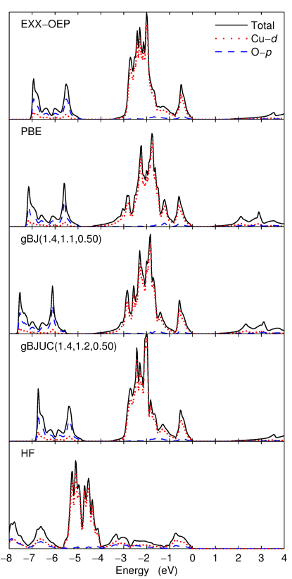
Figure 4: (Color online) DOS of Cu₂O. The Fermi energy is set at zero.

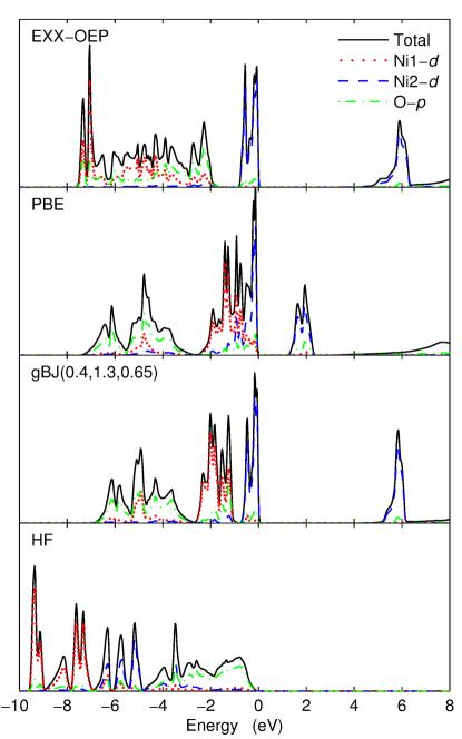
Figure 5: (Color online) Spin-up DOS of NiO. The Fermi energy is set at zero.

The comparison of the electronic structure obtained with the different exchange potentials focussed so far on the transition energies and the core states. In order to assess the differences in the electronic structure on a wider energy spectrum of the valence states, we compare the density of states of NiO and Cu₂O around the Fermi energy. We picked out these two solids from our test set, since the largest changes in the DOS with respect to the applied potential can be observed for these two solids. For C, Si, BN, and MgO the basic structure of the DOS remains very similar independent from the applied potential (of course, apart from a rigid shift of the conduction bands).

Figures 4 and 5 show the DOS of Cu₂O and NiO, respectively, for a few selected potentials. In the case of Cu₂O, we can clearly see that the gBJUC$(1.4,1.2,0.50)$ potential (very good for the transition energies and EFG, see below) leads to the best agreement with EXX-OEP, which is particularly true for the partial Cu-$3d$ DOS in the range from $-3$ to 0 eV below the Fermi energy. The Cu-$3d$ DOS obtained with the other semilocal potentials, including gBJ without UC, are too broad by about 1 eV. gBJUC$(1.4,1.2,0.50)$ also leads to correct positions of both the O-$2p$ (extending from $-7$ to $-5$ eV) and the conduction band Cu-$4s$ states. The HF DOS differs significantly from the other calculations employing a local exchange potential including EXX-OEP. It is well known that the HF method systematically leads to band gaps which are by far too large compared to experiment. In the case of Cu₂O, the HF band gap amounts to 10.4 eV, while it is only 2.17 eV in experimentBaumeister (1961) and 1.44 eV with EXX-OEP. In the occupied part of the spectrum, it is obvious that the main position of the Cu-$3d$ peaks are much lower in energy (below $-4$ eV), while the bands in the energy range from $-4$ to 0 eV are a mixture of Cu-$3d$ and O-$2p$ states. For other systems, a comparison between the HF and EXX-OEP occupied spectrum can be found in, e.g., Refs. Kümmel and Kronik, 2008; Luo et al., 2012; Kohut et al., 2014.

For NiO, the semilocal methods lead to DOS that differ markedly from the EXX-OEP DOS. As already discussed in Refs. Engel and Schmid, 2009; Betzinger et al., 2013 the spin-up highest valence bands (between $-0.8$ and 0 eV) and lowest conduction bands in the EXX-OEP DOS are of Ni-$3d$ character coming from the Ni atom with more spin-down electrons (Ni2 with $t_{2g}^{\uparrow}$ occupied and $e_{g}^{\uparrow}$ emtpy), while the spin-up states between $-7.5$ and $-2$ eV are mixtures of Ni-$3d$ from the Ni atom Ni1 ($t_{2g}^{\uparrow}$ and $e_{g}^{\uparrow}$ fully occupied) and O-$2p$. Therefore, EXX-OEP leads to a clear energy separation between the spin-up and spin-down Ni-$3d$ states of the same Ni atom. In the PBE DOS the position of the conduction states is much too low and there is no Ni-$3d$ peak similar to the one at $\sim-7.5$ eV in the EXX-OEP DOS. In addition, there is very little energy separation between the spin-up $3d$ states coming from the two Ni atoms. The gBJ$(0.4,1.3,0.65)$ potential leads to a good band gap and a separation of $\sim 0.5$ eV between the spin-up $3d$ states from the two Ni atoms, however, there is still no Ni-$3d$ peak at the lower part of the valence DOS, which can only be obtained by the LDA+$U$Anisimov et al. (1991) or HF/hybridTowler et al. (1994); Bredow and Gerson (2000); de P. R. Moreira et al. (2002); Tran et al. (2006) methods. We mention that the gBJ potentials with small values of $c$ (1.0 or 1.1) and the gBJUC potentials do not produce any energy separation between the $3d$ states of the two Ni atoms. The valence part of the HF DOS starts at $-10$ eV and about five sharp Ni-$3d$ peaks are equally distributed in the energy range $-10$ to $-5$ eV, while the DOS from $-3$ to 0 eV is exclusively of O-$2p$ character. The HF band gap is 13.9 eV, which is in fair agreement with previous HF results.Towler et al. (1994); Bredow and Gerson (2000); de P. R. Moreira et al. (2002) In experiment, a gap of 4.0-4.3 eV is observed,Hüfner et al. (1984); Sawatzky and Allen (1984) while EXX-OEP gives rise to 3.54 eV.

IV.3 EFG of Cu₂O and magnetic moment in NiO

Table 4: Spin magnetic moment $\mu_{S}^{\text{Ni}}$ (in $\mu_{\text{B}}$) inside the Ni atomic sphere of radius 1.016 Å in NiO and EFG of Cu (in $10^{21}$ V/m²) in Cu₂O.

		EFG${}_{\text{Cu}}$
Method	$\mu_{S}^{\text{Ni}}$	Total	$p$-$p$	$d$-$d$
EXX-OEP	1.91	$-17.7$	$-25.0$	7.2
LDA	1.30	$-4.7$	$-15.7$	10.8
PBE	1.43	$-5.6$	$-16.3$	10.5
B88	1.43	$-5.6$	$-16.3$	10.5
EV93	1.51	$-6.8$	$-17.5$	10.4
AK13	1.58	$-8.1$	$-18.5$	10.1
BJ	1.53	$-7.4$	$-17.7$	10.2
BJUC	1.41	$-11.3$	$-19.4$	7.9
gBJ$(0.6,1.0,0.60)$	1.61	$-7.0$	$-17.6$	10.5
gBJ$(1.4,1.1,0.50)$	1.66	$-8.3$	$-19.3$	10.8
gBJ$(0.4,1.3,0.65)$	1.86	$-5.1$	$-18.2$	13.0
gBJUC$(1.4,1.2,0.50)$	1.59	$-15.1$	$-22.2$	6.8
HF	1.88	$-17.0$	$-25.0$	7.9
Expt.	$1.90\pm 0.2$	9.8

As shown in Refs. Blaha et al., 1988; Schwarz et al., 1990 the EFG is mainly determined by the non-spherical electron density close to the nucleus. Since the density of the core electrons is (by construction) purely spherical, it is the electron density of the valence states that determines the EFG. Moreover, in the case of a $3d$-transition metal like Cu, the valence electron density in a region of a few tenths of an Angstrom from the nucleus is decisive. Hence, by comparing the EFG of Cu₂O for the different potentials we indirectly measure the difference in the non-spherical part of the valence electron density. The results for the EFG of Cu are shown in Table 4. Similarly to the transition energies in Cu₂O (see Sec. IV.2.1), only the gBJ potential with the UC (gBJUC) is able to reproduce the EXX-OEP EFG qualitatively. For instance, with the parameters $(1.4,1.2,0.50)$, gBJUC leads to an EFG of $-15.1\times 10^{21}$ V/m², while for all other potentials (except BJUC), the magnitude of the EFG does not exceed $10\times 10^{21}$ V/m². For gBJUC$(1.4,1.2,0.50)$, not only the total EFG, but also its two main components ($p$-$p$ and $d$-$d$) agree rather well with the EXX-OEP (and HF) values (see Table 4). A detailed analysis of the UC will be provided in Sec. IV.4. A calculation with the non-multiplicative HF potential leads to an EFG of $-17.0\times 10^{21}$ V/m² which is relatively close to the EXX-OEP value and expected since the first-order change in the electron density due to the replacement $v_{\text{x},i}^{\text{HF}}\rightarrow v_{\text{x}}^{\text{EXX-OEP}}$ is zero.Krieger et al. (1992a); Grabo et al. (2000); Kümmel and Perdew (2003) The magnitude of the experimental EFG amounts to $9.8\times 10^{21}$ V/m² (Refs. Kushida et al., 1956; Pyykkö, 2001), which is much smaller than the EXX-OEP or HF values. Thus, the impact of the electron correlation on the EFG is significant: the EXX-OEP value has to be reduced by the exact correlation functional nearly by its half. Furthermore, it was shown in Refs. Hu et al., 2008; Scanlon et al., 2009; Scanlon and Watson, 2010; Tran and Blaha, 2011; Koller et al., 2011 that the LDA, GGA, LDA+$U$, onsite-hybrid,Novák et al. (2006); Tran et al. (2006) and mBJ methods lead to an EFG in Cu₂O which is by far too small. The experimental value could only be approached with full hybrid functionals.

Next we turn the discussion to the spin magnetic moment $\mu_{S}^{\text{Ni}}$ of Ni in NiO (results in Table 4). In contrast to the EFG, $\mu_{S}^{\text{Ni}}$ is determined by the difference of the spherical spin-up and -down electron densities in the atomic spheres. The best agreement with the EXX-OEP Ni spin magnetic moment is obtained by the gBJ potential with a $c$ parameter of at least 1.2, which is in accordance with the observations for the EXX total energy and transition energies in Secs. IV.1 and IV.2.1. In fact, the parameters $(0.4,1.3,0.65)$ of the gBJ potential lead to $\mu_{S}^{\text{Ni}}=1.86$ $\mu_{\text{B}}$, which is very close to the EXX-OEP, HF, and experimental values. All other investigated potentials substantially underestimate the EXX-OEP spin-magnetic moment.

IV.4 Analysis of the potentials

Figure 6: (Color online) Two-dimensional plots of exchange potentials $v_{\text{x}}$ in a $(110)$ plane of C. The potentials were shifted such that $\int_{\text{cell}}v_{\text{x}}(\mathbf{r})d^{3}r=0$. The contour lines start at $-2$ Ry (blue color) and end at 1 Ry (red color) with an interval of 0.2 Ry.

\begin{picture}(8.0,13.1)(0.0,0.0)\put(0.0,6.5){\epsfbox{fig_1D_Si_vx_a.pdf}} \put(0.0,0.0){\epsfbox{fig_1D_Si_vx_b.pdf}} \end{picture}

Figure 7: (Color online) Exchange potentials $v_{\text{x}}$ in Si plotted from the vicinity of the atom at site $(1/8,1/8,1/8)$ ($d=0$) to (a) the center of the unit cell ($d=3.53$ Å) or (b) the mid-distance to the atom at site $(5/8,5/8,1/8)$ ($d=2.38$ Å). The potentials were shifted such that $\int_{\text{cell}}v_{\text{x}}(\mathbf{r})d^{3}r=0$.

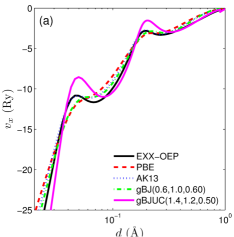
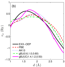
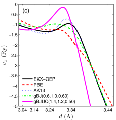
Figure 8: (Color online) Exchange potentials $v_{\text{x}}$ in Cu₂O plotted from the Cu atom at site $(1/2,1/2,0)$ ($d=0$) in the direction of the O atom at site $(3/4,3/4,3/4)$ ($d=3.54$ Å). Logarithmic scales on the $x$-axis were used for panels (a) and (c) which correspond to the vicinity of the Cu and O atoms, respectively. The potentials were shifted such that $\int_{\text{cell}}v_{\text{x}}(\mathbf{r})d^{3}r=0$.

\begin{picture}(8.0,14.0)(0.0,0.0)\put(0.0,6.9){\epsfbox{fig_1D_Cu2O_clmval20.pdf}} \put(0.0,0.0){\epsfbox{fig_1D_Cu2O_r2v20.pdf}} \end{picture}

Figure 9: (Color online) Plots of the radial functions $\rho_{20}$ (a) and $v_{\text{x},20}$ (b) versus the distance from the Cu atom in Cu₂O. The functions are multiplied by $r^{2}$.

Figure 10: (Color online) Two-dimensional plots of the difference between spin-up and spin-down exchange potentials ($v_{\text{x}}^{\uparrow}-v_{\text{x}}^{\downarrow}$) in a $(001)$ plane of antiferromagnetic NiO. The contour lines start at $-2$ Ry (blue color) and end at 2 Ry (red color) with an interval of 0.235 Ry. The Ni atom with a full spin-up $3d$-shell is at the left upper corner.

In the following, the results of the previous subsections are set in relation to the spatial form of the different exchange potentials. We start with discussing the exchange potential of C in the (110) plane (see Fig. 6). Since the LDA potential depends only on the electron density $\rho$, the corresponding contour plot is the most structureless. In comparison to the other potentials it exhibits a more spherical shape around the C atoms and is less corrugated in the interstitial region. It is less attractive (i.e., negative) than EXX-OEP in the bonding region, but more attractive in the interstitial. Therefore, compared to LDA there is a transfer of electrons from the interstitial to the bonding region with EXX-OEP (see Sec. IV.5). The GGA potentials (PBE, B88, EV93, and AK13), that depend additionally on the first and second derivatives of $\rho$, show stronger spatial variations. For example, the PBE potential is more undulated than LDA, but features seen in the EXX-OEP are still reproduced too weakly or completely missing. (B88 is not shown since its contour plot is very similar to the PBE plot.) The GGA potentials EV93 and AK13 as well as the gBJ potential are more anisotropic. The gBJ potentials leads to an improved agreement with EXX-OEP both in the bonding and interstitial regions, whereas the EV93 and AK13 potentials show too much variation in the interstitial region. We note that similar conclusions can be drawn for Si, BN, and MgO.

However, it is also clear from Fig. 6 that the agreement between EXX-OEP and the best semilocal potentials (gBJ) is not perfect and that differences are still present. For a more detailed analysis we show in Fig. 7 one-dimensional potentials plots for Si. It becomes evident from Fig. 7(a) that AK13 (and to a lesser extent also EV93) leads to completely unphysical oscillations in the interstitial region of Si, while the EXX-OEP and gBJ potentials are rather flat and very similar to each other in this region. Actually, we have observed that in general the AK13 and EV93 potentials show such large oscillations in the wide interstitial regions present in such open structures, which is due to their enhancement factors $F_{\text{x}}\left(s\right)$ in Eq. (7) whose magnitudes are much larger than for PBE and B88 (see Fig. 1). The direct effect of these much more positive values of the AK13 potential in the interstitial region is to shift up the unoccupied orbitals (located mainly in the interstitial) relative to the occupied ones, thus explaining the positive (or less negative than for most other potentials) AK13 values for the ME on the transition energies (Table 2).

In Fig. 7(b) we can see that the height of the intershell peak at $d\sim 0.6$ Å is strongly underestimated and washed-out by PBE, whereas EV93 and AK13 tend to overestimate the peak height for Si. However, with increasing atomic number the ability of the AK13 and EV93 potentials to reproduce the height and position of the intershell peaks seems to improve. As shown in Fig. 8, in the vicinity of the Cu atom both AK13 and EV93 mimic the EXX-OEP quite accurately, while substantial differences are present at the O atom [see Fig. 8(c)]. Similar observations hold for the intershells peaks in NiO. This is in agreement with Refs. Engel and Vosko, 1993b; Armiento and Kümmel, 2013 which show that AK13 and EV93 reproduce very accurately the position and height of the intershells peaks in transition-metal atoms. As already discussed in Sec. II.2 and shown in Fig. 2, the height and position of the peaks with gBJ depend strongly on the three parameters $\gamma$, $c$, and $p$. As shown in Fig. 7(b), the intensity of the peak is too large with $(\gamma,c,p)=(1.4,1.1,0.50)$, but too weak with $(\gamma,c,p)=(0.6,1.0,0.60)$ (not shown).

Concerning the BJ-based potential with the UC, gBJUC, the results are very bad for the EXX total energy and energy position of core states as discussed above (see Tables 1 and 3). This is a consequence of the very inaccurate gBJUC potential in the region close to the nuclei as shown in Figs. 8(a) and 8(c). As discussed in Sec. II.2, the effect of replacing the kinetic-energy density $t$ by $D$ in the second term of Eq. (16) is very large in the core region of atoms with the consequence that the potential becomes too attractive. On the contrary, without the UC the gBJ potential resembles the EXX-OEP very closely in the core region [except at the position of the intershell peaks, see Figs. 8(a) and 8(c)].

Though, for Cu₂O it was mandatory to use the UC in order to obtain qualitative agreement with EXX-OEP for the transition energies and EFG. For the EFG in particular, this could seem puzzling that the gBJUC potential gives good results despite it looks quite inaccurate close to the Cu nucleus. However, as already mentioned in Sec. IV.3, the EFG is determined by the non-sphericity of the electron density $\rho$ near the nucleus. More specifically, the EFG is determined essentially by the radial function $\rho_{LM}$ with $\left(L,M\right)=\left(2,0\right)$ of the spherical harmonics expansion of the electron density inside the atomic sphere.Blaha et al. (1988) Figure 9(a) shows the (expected) very good agreement between the gBJUC, EXX-OEP, and HF methods for $\rho_{20}$ (and also for $\rho_{40}$ but not $\rho_{00}$). By looking at the corresponding radial function $v_{\text{x},20}$ of the exchange potential [see Fig. 9(b)], we can observe a rather good agreement between gBJUC and EXX-OEP in the region beyond 0.2 Å, which mainly concerns the $d$-$d$ component of the EFG (see Table 4). We mention that the radial functions $\rho_{20}$ and $v_{\text{x},20}$ obtained with B88, EV93, and AK13 are qualitatively similar to PBE and gBJ without UC. For the $p$-$p$ component, the agreement between gBJUC and EXX-OEP also comes from the valence region of the Cu atom and the interstitial, and, as shown in Fig. 8(b), these two potentials are relatively close to each other in this region. Actually, the correct description of the Cu-$p$ states far away from the Cu nucleus affects the anisotropy of the Cu-$p$-states close to the Cu nucleus. These similarities observed in the EXX-OEP and gBJUC potentials can also explain the agreement for the transition energies.

Turning to antiferromagnetic NiO, the difference $v_{\text{x}}^{\uparrow}-v_{\text{x}}^{\downarrow}$ between the spin-up and spin-down exchange potentials is shown in Fig. 10. The angular $e_{g}$-shape around the Ni atoms is the most pronounced with the EXX-OEP and gBJ [with $(\gamma,c,p)=(0.4,1.3,0.65)$] potentials, thus leading to the large band gaps between the $t_{2g}$ and $e_{g}$ states of the minority spin (see DOS in Fig. 5) in comparison to the other potentials. However, it can also be observed that the magnitude of $v_{\text{x}}^{\uparrow}-v_{\text{x}}^{\downarrow}$ is the largest with EXX-OEP (i.e., compared to gBJ there are a couple of additional isolines between the Ni and O atoms), which could explain the large exchange splitting between the spin-up and spin-down states observed in Fig. 5 for EXX-OEP.

IV.5 Analysis of the electron density

Figure 11: (Color online) Electron density $\rho$ obtained with different exchange potentials minus $\rho^{\text{LDA}}$ plotted in a $(110)$ plane of Si. The contour lines start at $-0.001$ electron/bohr³ (blue color) and end at 0.001 electron/bohr³ (red color) with an interval of 0.0002 electron/bohr³.

Figure 12: (Color online) Spin-up electron density $\rho_{\uparrow}$ obtained with different exchange potentials minus $\rho_{\uparrow}^{\text{LDA}}$ plotted in a $(001)$ plane of antiferromagnetic NiO. The contour lines start at $-0.005$ electron/bohr³ (blue color) and end at 0.005 electron/bohr³ (red color) with an interval of 0.001 electron/bohr³. The Ni atom with a full spin-up $3d$-shell is at the left upper corner.

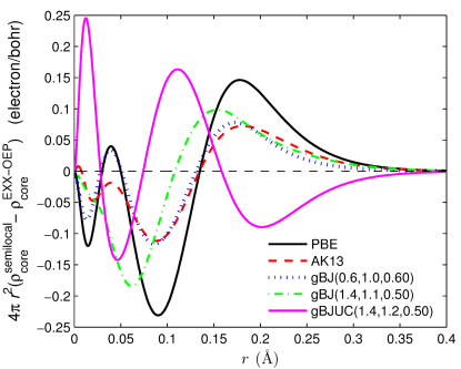
Figure 13: (Color online) The difference between the density $\rho_{\text{core}}$ of the core electrons of Cu in Cu₂O calculated with semilocal functionals and $\rho_{\text{core}}$ from EXX-OEP (multiplied by $4\pi r^{2}$).

Figure 11 shows the electron density in Si obtained from various potentials minus the LDA density, which serves as reference. As discussed above for the case of C (Fig. 6), which is very similar to Si and BN, the GGA, gBJ, and EXX-OEP potentials are more attractive (repulsive) than LDA in the bonding (interstitial) region of Si. Consequently, the electron density is increased (decreased) in the bonding (interstitial) region. From Fig. 11 it is rather clear that the gBJ and EXX-OEP potentials lead to very similar electron densities, while the EV93 and AK13 densities are, compared to EXX-OEP, too large (small) in the bonding (interstitial) regions.

As shown in Fig. 12 for NiO, the effect of using a beyond-LDA potential is to increase the spin-up electron density $\rho_{\uparrow}$ on the Ni atom with a full spin-up $3d$-shell (red regions around the Ni atom at the left upper corner) and to decrease the spin-down density $\rho_{\downarrow}$ on the same Ni atom (which corresponds to $\rho_{\uparrow}$ around the other Ni atom). This results in an increase of the magnetic moment of the Ni atom as discussed above (see Table 4). The other effect of using a beyond-LDA potential is to increase the ionicity (red regions around the O atoms). More quantitatively, compared to LDA the number of electrons inside the sphere of the Ni atom changes by $+0.01$ (PBE), $-0.01$ (EV93, AK13), $-0.14$ [gBJ$(0.4,1.3,0.65)$], and $-0.11$ (EXX-OEP), while for the O atom the changes are $+0.10$ (PBE), $+0.16$ (EV93), $+0.23$ (AK13), $+0.47$ [gBJ$(0.4,1.3,0.65)$], and $+0.35$ (EXX-OEP), which shows that gBJ reproduces quite accurately the trends of EXX-OEP. From Fig. 12, it is also rather clear that the gBJ$(0.4,1.3,0.65)$ and EXX-OEP electron densities are overall very similar (note in particular the asymmetry of the $3d$ density around the Ni atom with partially filled spin-up electrons).

In Fig. 13 we show the density of the core electrons of the Cu atom in Cu₂O. Compared to the density $\rho_{\text{core}}$ obtained with EXX-OEP, the PBE core density is less contracted since it has smaller values for $r<0.14$ Å but is larger for $r>0.14$ Å. The reverse is true for the gBJUC potential since the positive values of $\rho_{\text{core}}^{\text{gBJUC}}-\rho_{\text{core}}^{\text{EXX-OEP}}$ are on average closer to the nucleus than the negative values, which is a consequence of the fact that close to the nuclei gBJUC is much more attractive than the EXX-OEP and all other potentials (as discussed in Secs. II.2 and IV.4). The AK13 and gBJ potentials lead to trends similar to PBE, however the discrepancies with respect to EXX-OEP are reduced. Note also that the gBJ potential with the parameters $(\gamma,c,p)=(0.6,1.0,0.60)$, which are more appropriate for the EXX total energy, leads to a slightly more accurate core density than with the values $(1.4,1.1,0.50)$ that were determined for the transition energies.

V Summary and outlook

In this work, we have compared several approximate semilocal exchange potentials to the exact EXX-OEP. The closeness between the semilocal and EXX-OEP potentials was quantified by considering the EXX total energy and electronic band structure for various solids, as well as the EFG in Cu₂O and the magnetic moment in NiO. An attempt to parameterize a semilocal BJ-based potential has also been made and we have shown that by the introduction of a few parameters, it was possible to improve substantially the agreement with EXX-OEP compared to the GGA and original BJ potentials. However, it became also obvious that there is no universal set of parameters that leads to satisfying results for all properties and solids at the same time. For instance, if a set of parameters is appropriate for the EXX total energy (or electronic structure) of C, Si, BN, and MgO, then it will not work so well for antiferromagnetic NiO, and vice-versa. Another example was Cu₂O for which it is mandatory to use the UC to obtain qualitative agreement with EXX-OEP for the band gap and EFG, while the UC is very detrimental for the EXX total energy and energy position of the core states in all solids.

From the results, it is clear but not surprising that although the BJ-based potentials lead to interesting results, the semilocal approximations show limitations and, furthermore, there is no systematic way to improve their accuracy. Beyond the semilocal level of theory, there is the group of exchange potentials which consist of the nonlocal Slater potential $v_{\text{x}}^{\text{S}}$ [Eq. (9)] plus a term which is either nonlocal [like in the Krieger-Li-Iafrate (KLI)Krieger et al. (1992b) or localized HF (LHF)Della Sala and Görling (2001); Gritsenko and Baerends (2001) potentials] or local with an eventual dependency on the energies of the occupied orbitals.Harbola and Sen (2002); Gritsenko et al. (1995) The computational cost of these potentials is rather high since the Slater potential and the nonlocal terms require the calculation of HF-type integrals (see Ref. Kohut et al., 2014 for a summary of the expression of these potentials). These nonlocal potentials avoid some of the technical difficulties of EXX-OEP as their construction involves only the occupied orbitals. There are numerous studies on the Slater-based potentials and we just mention Ref. Ryabinkin et al., 2013 where it was shown that the KLI- and LHF-generated orbitals lead to EXX total energy of atoms which are much lower than with BJ orbitals. However, Engel (Ref. Engel and Schmid, 2009) noted that the KLI approximation is not able to open the band gap in antiferromagnetic FeO, while a band gap of 1.66 eV is obtained with EXX-OEP (augmented by LDA for correlation).

On the other hand, as already mentioned in Sec. II.2, the semilocal BR potentialBecke and Roussel (1989) [Eq. (10)] seems to reproduce (at least visually) quite accurately the features of the Slater potential in atoms, Becke and Roussel (1989); Becke and Johnson (2006) however, the agreement is not perfect (see Ref. Karolewski et al., 2013) and the comparison of the EXX total energies evaluated with BJ(Slater) and BJ(BR) orbitals shows non-negligible differences in some cases.Becke and Johnson (2006) Avoiding the calculation of the Slater potential by using the BR potential instead would certainly be advantageous, but more comparison studies between the BR and Slater potentials are needed.

A possible way of improving the reliability of a semilocal potential (e.g., gBJ) to reproduce EXX-OEP, could be to use a similar parameterization as the one used for the constant $c$ in the mBJ potentialTran and Blaha (2009) [Eq. (15)]:

$$c=\alpha+\beta\left(\frac{1}{V_{\text{cell}}}\int\limits_{\text{cell}}\frac{\left|\nabla\rho(\mathbf{r})\right|}{\rho(\mathbf{r})}d^{3}r\right)^{1/2},$$ (17)

where $\alpha$ and $\beta$ are parameters and $V_{\text{cell}}$ is the unit cell volume. It has been shown that with the optimized values $\alpha=-0.012$ and $\beta=1.023$ bohr^1/2, mBJ reproduces with rather great accuracy the experimental band gap of many solids. Tran and Blaha (2009); Singh (2010); Koller et al. (2011, 2012) Actually, the use of an integral expression like Eq. (17) is a way to introduce nonlocality (similar as with the Slater potential), but in a cheap way since there is no summation over orbitals like in the Slater potential. However, the drawback of using the average of $\left|\nabla\rho\right|/\rho$ in the unit cell is that this quantity is infinite for systems with an infinite vacuum (e.g., isolated molecule or surface). An alternative to Eq. (17) which can be applied to any kind of systems might be helpful in improving the universal character of a potential like gBJ. For instance, as suggested by Marques et al. in Ref. Marques et al., 2011, a possibility would be to make $c$ $\mathbf{r}$-dependent and the integrand in Eq. (17) localized around $\mathbf{r}$ by multiplying $\left|\nabla\rho\right|/\rho$ by a function of $\left|\mathbf{r}-\mathbf{r}^{\prime}\right|$ which goes to zero at $\left|\mathbf{r}-\mathbf{r}^{\prime}\right|\rightarrow\infty$.

In order to adjust the parameters of an approximate functional for each system, an approach as suggested in Ref. Yang and Wu, 2002 might be helpful. The free parameters of the potential are adapted at each iteration such that the EXX total energy becomes minimal. However, such a procedure is rather expensive since the equations to determine the parameters involve HF-like matrix elements between occupied and unoccupied orbitals. Nevertheless, this would be a way to adjust the parameters for each solid and therefore improve the universality of the potential.

Moreover, we mention the work of Staroverov and co-workers Ryabinkin et al. (2013); Kohut et al. (2014) who proposed an expression for a multiplicative exchange potential (making no use of unoccupied orbitals) which leads to results that are quasi-identical to the EXX-OEP results. However, this approach requires the HF orbitals which reduces its use for solids and large scale applications.

Finally, we note the very few studies reporting OEP calculations including correlation like the random-phase approximation (RPA) in addition to EXX (see Refs. Kotani and Akai, 1998; Kotani, 1998; Grüning et al., 2006, 2006; Klimes and Kresse, 2014 for results on solids). The RPA-OEP potentials could certainly also serve as reference for the modelling of realistic multiplicative exchange-correlation potentials $v_{\text{xc}}$ including correlation.