Some numerical results on the behavior of zeros of the Hermite–Padé polynomials

Abstract.

We introduce and analyze some numerical results obtained by the authors experimentally. These experiments are related to the well known problem about the distribution of the zeros of Hermite–Padé polynomials for a collection of three functions $[f_{0}\equiv 1,f_{1},f_{2}]$. The numerical results refer to two cases: a pair of functions $f_{1},f_{2}$ forms an Angelesco system (see (3)) and a pair of functions $f_{1}=f,f_{2}=f^{2}$ forms a (generalized) Nikishin system (see (4)). The authors hope that the obtained numerical results will set up a new conjectures about the limiting distribution of the zeros of Hermite–Padé polynomials.

Bibliography: [71] titles; 79 pictures.

Keywords: rational approximations, Padé approximants, Stahl compact set, Hermite–Padé polynomials, Nuttall condenser, distribution of zeros, Froissart doublets, Angelesco system, Nikishin system, singlets, triplets, Froissart phenomenon

1. Introduction

1.1.

In the present work we introduce and analyze some numerical results obtained by experimenting. These experiments are connected with the well known problem about the distribution of the zeros of Hermite–Padé polynomials for a collection of three functions $[f_{0}\equiv 1,f_{1},f_{2}]$, defined and holomorphic at the infinity point $z=\infty$, $f_{1},f_{2}\in\mathscr{H}(\infty)$. Our numerical experiments are restricted only to the Hermite–Padé polynomials of first kind. It is well known that Hermite–Padé polynomials of first and second kind are closely related to each other, see [46, §2, equation (2.1.9)], [13], [14], [15]. The numerical results obtained here may permit interpretations about the Hermite–Padé polynomials of the second kind.

Let $\mathbb{P}_{n}:=\mathbb{C}_{n}[z]$, $n\in\mathbb{N}$, be the class of all polynomials with complex coefficients of degree $\leqslant{n}$. For an arbitrary $n\in\mathbb{N}$, define the Hermite–Padé polynomials of first kind $Q_{n,j}\in\mathbb{P}_{n}$, $j=0,1,2$, $Q_{n,1},Q_{n,2}\not\equiv 0$, by the relation (see [46], also [24], [60], [28], [2], [8], [3], [14])

(1) $$(Q_{n,0}\cdot 1+Q_{n,1}f_{1}+Q_{n,2}f_{2})(z)=O\left(\frac{1}{z^{2n+2}}\right),\qquad z\to\infty.$$

In the present work, we will use the terminology and notation of the work by J. Nuttall [46] (see also H. Stahl [60]). According to their paper, the classical Padé polynomials $P_{n,0},P_{n,1}$ of the function $f\in\mathscr{H}(\infty)$ are, in fact, the Hermite–Padé polynomials for the collection of two functions $[f_{0}\equiv 1,f_{1}=f]$, such that $P_{n,0},P_{n,1}\in\mathbb{P}_{n}$, $P_{n,1}\not\equiv 0$ and:

(2) $$(P_{n,0}\cdot 1+P_{n,1}f)(z)=O\left(\frac{1}{z^{n+1}}\right),\qquad z\to\infty.$$

We present the results from our numerical experiments about two cases.

In the first case the functions $f_{1}$ and $f_{2}$ have the following form:

(3) $$f_{1}(z)=\frac{z}{\sqrt{(z-a_{1})(z-b_{1})}},\qquad f_{2}(z)=\frac{z}{\sqrt{(z-a_{2})(z-b_{2})}},$$

where $a_{1},b_{1},a_{2},b_{2}\in\mathbb{C}$, $a_{1}\neq b_{1}$, $a_{2}\neq b_{2}$, and $\{a_{1},b_{1}\}\cap\{a_{2},b_{2}\}=\varnothing$. Therefore, the pair of functions $f_{1},f_{2}$ forms an Angelesco system (see [36], [24], [60], [27], [28], [2]).

In the second case, $f_{1}=f$, $f_{2}=f^{2}$, where

(4) $$f(z)=(z^{2}-1)^{1/4}(z-a)^{-1/2},\quad f(\infty)=1,\quad a\not\in\mathbb{R},$$

and the pair of functions $f_{1},f_{2}$ forms a (generalized) Nikishin system (see [43], [27], [28], [2], [5], [49], [34], [35]).

Remark 1.

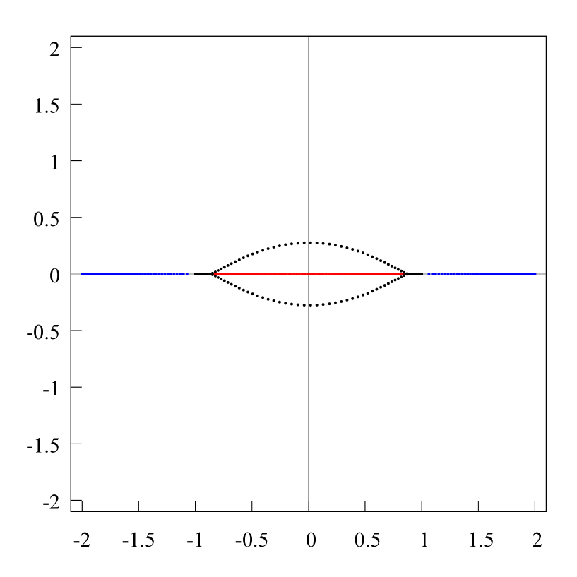
Figure 15. The distribution of the zeros of the Hermite-Padé polynomials $Q_{120,0}$ (blue points), $Q_{120,1}$ (red points) and $Q_{120,2}$ (black points) for a set of three functions $[1,f_{1},f_{2}]$, where $f_{1}(z)=\left((z-1)/(z+1)\right)^{1/3}\left((z-2)/(z+2)\right)^{1/3}$, $f_{2}(z)=\left((z-1)/(z+1)\right)^{2/3}\left((z-2)/(z+2)\right)^{1/3}$. The pair $f_{1},f_{2}$ create a Nikishin system, because the branch points of the functions are equivalent. However, the distribution of the zeros of the Hermite-Padé polynomials for this system is the same as the distribution of the zeros for the Angelesco system $f_{1}(z)=\sqrt{(z-1)/(z+1)}$, $f_{2}(z)=\sqrt{(z-2)/(z+2)}$; see fig. 14, 16, 17.

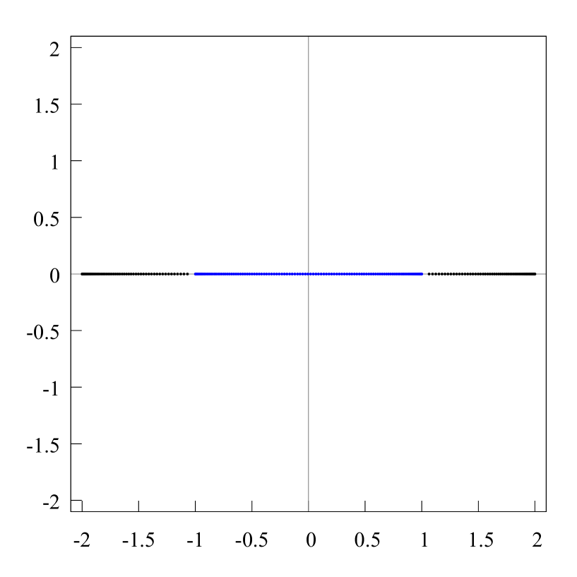
Figure 16. The distribution of the zeros of the Hermite-Padé polynomials $Q_{120,0}$ (blue points) and $Q_{120,2}$ (black points) for a set of three functions $[1,f_{1},f_{2}]$, where $f_{1}(z)=\sqrt{(z-1)/(z+1)}$, $f_{2}(z)=\sqrt{(z-2)/(z+2)}$. The pair $f_{1},f_{2}$ create an Angelesco system. However, the distribution of the zeros of the Hermite-Padé polynomials for this system is the same as the distribution for the Nikishin system $f_{1}(z)=\left((z-1)/(z+1)\right)^{1/3}\left((z-2)/(z+2)\right)^{1/3}$, $f_{2}(z)=\left((z-1)/(z+1)\right)^{2/3}\left((z-2)/(z+2)\right)^{1/3}$; comp. fig. 17.

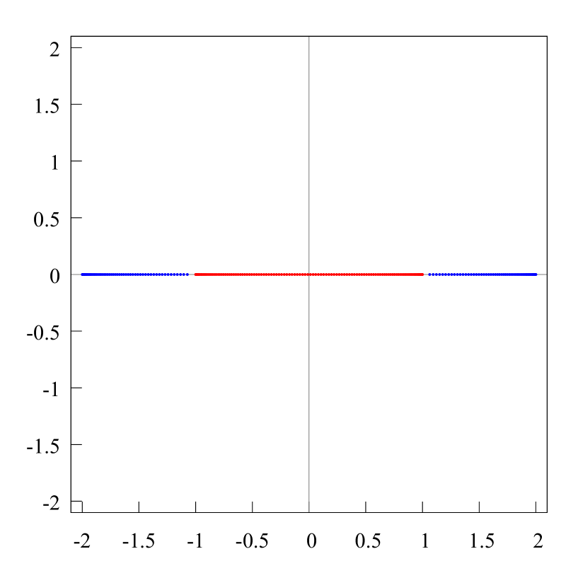
Figure 17. The distribution of the zeros of the Hermite-Padé polynomials $Q_{120,0}$ (blue points) and $Q_{120,1}$ (red points) for a set of three functions $[1,f_{1},f_{2}]$, where $f_{1}(z)=\left((z-1)/(z+1)\right)^{1/3}\left((z-2)/(z+2)\right)^{1/3}$, $f_{2}(z)=\left((z-1)/(z+1)\right)^{2/3}\left((z-2)/(z+2)\right)^{1/3}$. The pair $f_{1},f_{2}$ create a Nikishin system. However, the distribution of the zeros of the Hermite-Padé polynomials for this system is the same as the distribution for the Angelesco system $f_{1}(z)=\sqrt{(z-1)/(z+1)}$, $f_{2}(z)=\sqrt{(z-2)/(z+2)}$; comp. fig. 16.

In the theory of Hermite–Padé polynomials for a collection of three functions $[1,f_{1},f_{2}]$ two opposite situations are usually selected, which are connected with the distribution of the branch points of the functions $f_{1}$ and $f_{2}$. In the first case the sets of branch points $\mathcal{A}_{1}=\mathcal{A}(f_{1})$ and $\mathcal{A}_{2}=\mathcal{A}(f_{2})$ do not intersect each other. We say that the pair of functions forms an Angelesco system, see [28], [2], [5]. In the second case the sets of branch points $\mathcal{A}_{1}$ and $\mathcal{A}_{2}$ of the functions $f_{1}$ and $f_{2}$ are equivalent. We say that two functions $f_{1},f_{2}$ forms a Nikishin system, see [43], [28], [2], [5]. In the first case the interaction matrix $M$ for the theory-potential-equilibrium vector problem is $M=\begin{pmatrix}2&1\\ 1&2\end{pmatrix}$. In the second case it is $M=\begin{pmatrix}2&-1\\ -1&2\end{pmatrix}$, see [25], [28], [2], [49]. The natural expectation is that such differences between the distribution of the branch points and the structure of the interaction matrices leads to essentially different limiting distributions of the zeros of the corresponding Hermite–Padé polynomials. However, this is not always the case. Figures 14, 15, 16 and 17 show the distribution of the zeros of the polynomials $Q_{120,0}$ (blue points), $Q_{120,1}$ (red points), $Q_{120,2}$ (black points) for two pair of functions: one with different branch points

(5) $$f_{1}(z)=\sqrt{(z-1)/(z+1)},\qquad f_{2}(z)=\sqrt{(z-2)/(z+2)}$$

and the other with coincident branch points

(6) $$f_{1}(z)=\left(\frac{z-1}{z+1}\right)^{1/3}\left(\frac{z-2}{z+2}\right)^{1/3},\quad f_{2}(z)=\left(\frac{z-1}{z+1}\right)^{2/3}\left(\frac{z-2}{z+2}\right)^{1/3}.$$

From the results on figures 14–17 it follows that the distribution of the zeros of Hermite–Padé polynomials for these two different systems of functions will be equivalent (with regard to the fact that supports of the limit measures for the polynomials $Q_{n,j}$ change over to each other). Note that the system (6) is a special case of a two Markov functions system, which was considered by E. A. Rakhmanov in [49]. The numerical results for the system (6) obtained here are in a good agreement with the results of E. A. Rakhmanov [49].

Remark 2.

Instead of the pair of functions (5) with second order branch points we can consider a pair of functions with arbitrary order of the branch points. For example, the pair of functions

(7) $$f_{1}(z)=\sqrt[3]{(z-1)/(z+1)},\qquad f_{2}(z)=\sqrt[3]{(z-2)/(z+2)}$$

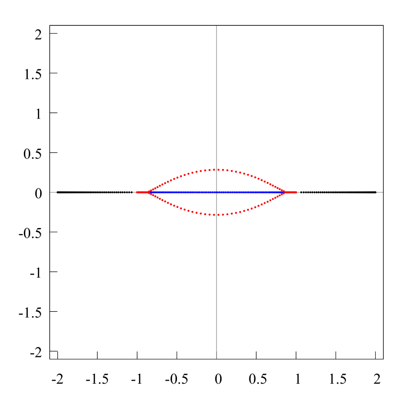
Figure 18. The distribution of the zeros of the Hermite-Padé polynomials $Q_{120,0}$ (blue points), $Q_{120,1}$ (red points) and $Q_{120,2}$ (black points) for a set of three functions $[1,f_{1},f_{2}]$, where $f_{1}(z)=\sqrt[3]{(z-1)/(z+1)}$, $f_{2}(z)=\sqrt[3]{(z-2)/(z+2)}$. The sets of branch points of the functions $f_{1}$ and $f_{2}$ do not intersect each other, and thus the pair $f_{1},f_{2}$ create an Angelesco system. However, the distribution of the zeros of the Hermite-Padé polynomials for this system is the same as the distribution for the Nikishin system $f_{1}(z)=\left((z-1)/(z+1)\right)^{1/3}\left((z-2)/(z+2)\right)^{1/3}$, $f_{2}(z)=\left((z-1)/(z+1)\right)^{2/3}\left((z-2)/(z+2)\right)^{1/3}$; see fig. 15–17.

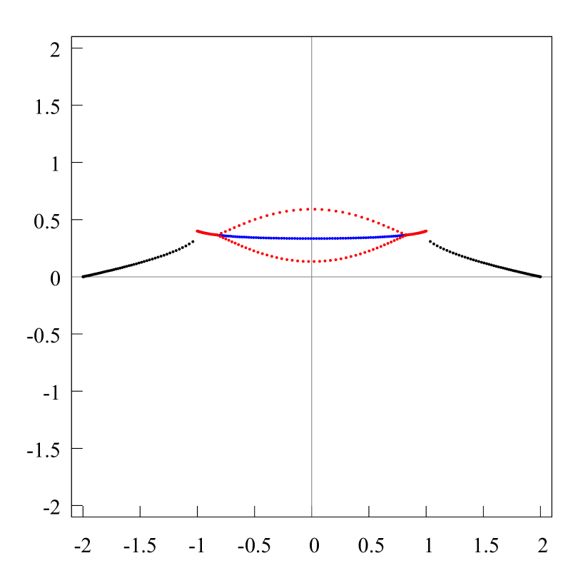
Figure 24. The distribution of the zeros of the Hermite-Padé polynomials $Q_{120,0}$ (blue points), $Q_{120,1}$ (red points) and $Q_{120,2}$ (black points) for a set of three functions $[1,f_{1},f_{2}]$, where $f_{1}(z)=\sqrt[3]{(z-(1+i\cdot 0.4))/(z-(-1+i\cdot 0.4))}$, $f_{2}(z)=\sqrt[3]{(z-2)/(z+2)}$. The set of the branch points of the functions $f_{1}$ and $f_{2}$ do not intersect each other, thus the pair $f_{1},f_{2}$ create an Angelesco system; comp. 18–20.

have the same distribution of the zeros of the corresponding Hermite–Padé polynomials as (5); see fig. 18–20 and comp. fig. 24–26. However, the pair of functions

(8) $$f_{1}(z)=\sqrt{(z-1)/(z+1)},\qquad f_{2}(z)=\sqrt[3]{(z-2)/(z+2)}$$

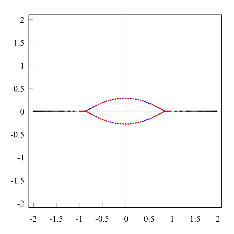
Figure 21. The distribution of the zeros of the Hermite-Padé polynomials $Q_{120,0}$ (blue points), $Q_{120,1}$ (red points) and $Q_{120,2}$ (black points) for a set of three functions $[1,f_{1},f_{2}]$, where $f_{1}(z)=\sqrt{(z-1)/(z+1)}$, $f_{2}(z)=\sqrt[3]{(z-2)/(z+2)}$. The sets of branch points of the functions $f_{1}$ and $f_{2}$ do not intersect each other, and thus the pair $f_{1},f_{2}$ create an Angelesco system. However, the distribution of the zeros of the Hermite-Padé polynomials for this system is different than the distribution of the pair $f_{1}(z)=\sqrt[3]{(z-1)/(z+1)}$, $f_{2}(z)=\sqrt[3]{(z-2)/(z+2)}$. comp. fig. 18–20. This confirms that the distribution of the zeros of the Hermite-Padé polynomials depends not only on the geometrical position of the branch points, but also of the type of the branch points.

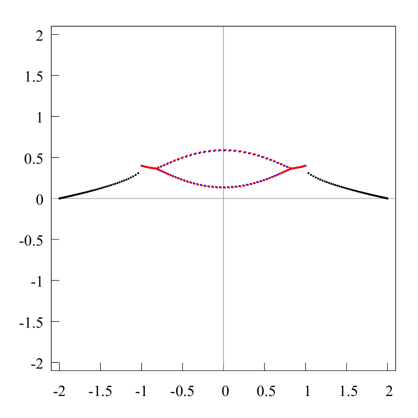
Figure 27. The distribution of the zeros of the Hermite-Padé polynomials $Q_{120,0}$ (blue points), $Q_{120,1}$ (red points) and $Q_{120,2}$ (black points) for a set of three functions $[1,f_{1},f_{2}]$, where $f_{1}(z)=\sqrt{(z-(1+i\cdot 0.4))/(z-(-1+i\cdot 0.4))}$, $f_{2}(z)=\sqrt[3]{(z-2)/(z+2)}$. The set of the branch points of the functions $f_{1}$ and $f_{2}$ do not intersect each other, thus the pair $f_{1},f_{2}$ create an Angelesco system; comp. 21–23.

have another distribution of the zeros of the corresponding Hermite–Padé polynomials, see fig. 21–23 and comp. fig. 27–29. Thus, the distribution depends non only of the type but also on the degree of the branch points (in (8) for the first function $f_{1}$ instead of degree $1/3$, as in (7), we took degree $1/2$).

The distribution of the zeros remains stable while moving the branch points of the function $f_{1}$ along the imaginary axis, for example, when we change the points $z=\pm 1$ into the points $z=\pm 1+i\cdot 0.4$:

(9) $$f_{1}(z)=\sqrt[3]{(z-(1+i\cdot 0.4))/(z-(-1+i\cdot 0.4))},$$

$$f_{2}(z)=\sqrt[3]{(z-2)/(z+2)},$$

see fig. 24–26 and comp. (7), and:

(10) $$f_{1}(z)=\sqrt{(z-(1+i\cdot 0.4))/(z-(-1+i\cdot 0.4))},$$

$$f_{2}(z)=\sqrt[3]{(z-2)/(z+2)},$$

see fig. 27–29 and comp. (8). This confirms that the distribution of the zeros of the Hermite–Padé polynomials depends not only on the geometrical position of the branch points, but also on the type of the branch points.

Remark 3.

If instead of (6) we consider the pair of functions

(11) $$f_{1}(z)=\left(\frac{z-1}{z+1}\right)^{1/3}\left(\frac{z-2}{z+2}\right)^{1/3},\quad f_{2}(z)=\left(\frac{z-1}{z+1}\right)^{2/3}\left(\frac{z-2}{z+2}\right)^{-1/3},$$

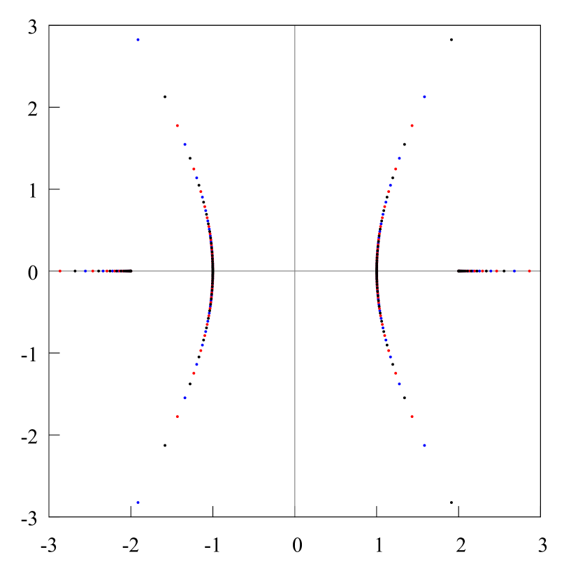
Figure 30. The distribution of the zeros of the Hermite-Padé polynomials $Q_{120,0}$ (blue points), $Q_{120,1}$ (red points) and $Q_{120,2}$ (black points) for a set of three functions $[1,f_{1},f_{2}]$, where $f_{1}(z)=\left((z-1)/(z+1)\right)^{1/3}\left((z-2)/(z+2)\right)^{1/3}$, $f_{2}(z)=\left((z-1)/(z+1)\right)^{2/3}\left((z-2)/(z+2)\right)^{-1/3}$. Here the pair $f_{1},f_{2}$ create a Nikishin system, because the branch points of the functions are equivalent.

then the distribution of the zeros of the corresponding Hermite–Padé polynomials will be different than before, see fig. 30–31.

1.2.

A numerous conjectures about the asymptotic behavior of the zeros of the Hermite–Padé polynomials of both first and second kind was, in part, formulated in the fundamental work of J. Nuttall [46] (see also [44], [45]). These conjectures served as a background for some of the numerous investigations. Among them the prominent results of H. Stahl [55]–[59] and A. A. Gonchar–E. A. Rakhmanov [24], [26], first of all should be noted, and also the results of A. I. Aptekarev with co-authors [1], [4], [2], [5], [6], [7]. J. Nuttall’s exact results [44], [45], [46] about the asymptotics of the Hermite–Padé polynomials for a collection of $m$ functions $[f_{0}\equiv 1,f_{1},\dots,f_{m-1}]$, $m\geqslant 3$, are based mainly on the a priori assumption of the existence of an associated $m$-sheeted Riemann surface $\mathfrak{R}_{m}$ with a canonical decomposition into $m$ sheets $\mathfrak{R}^{(j)}$, $j=1,\dots,m$. The sheets defined by an Abel integral of third kind with purely imaginary periods and logarithmic singularities of the form $(m-1)\log{z}$, $z=z^{(1)}\sim\infty^{(1)}$ and $-\log{z}$, $z=z^{(j)}\sim\infty^{(j)}$, $j=2,\dots,m$, and having also property that the first “physical” sheet $\mathfrak{R}^{(1)}$ is always connected (see [44], [46], [48]). In such case it is possible to describe the asymptotical behavior of the Hermite–Padé polynomials in terms connected to this RS (see [46], [47], [4], [2]). However, the question how to “construct” such a RS in the general case when $m\geqslant 3$ remains open. As for the present, results are achieved only for the case $m=3$. There are two major methods to obtain the results of such type. The first one mainly based on the cubic equation (see [1], [4], [10], also [47], [41], [42]). Using this method one can find an explicit representation of the so-called Nuttall’s $\phi$-function (see [4], [10], [11]), i.e., an Abel integral of third kind, which has the level curves that define the needed canonical decomposition of RS $\mathfrak{R}_{3}$ into three sheets . The other method consists of first solving the theoretical-potential extremal problem, connected with the existence of the so-called Nuttall condenser on the Riemann sphere $\overline{\mathbb{C}}$ (see [50], [51], [38], [71]). If such a condenser can be found, then the RS $\mathfrak{R}_{3}$ with the needed decomposition into three sheets is “constructed” on the base of this condenser by a specific scheme (see [51], [38]). Note that for now the second method can be applied only when the pair $f_{1},f_{2}$ forms a Nikishin system [51], [71]. Namely, for some general enough functions $f_{1},f_{2}$, which forms a complex Nikishin system, in [51] (see also [50], [38]) an existence of the Nuttall condenser, consisting of two non-intersecting plates and having certain symmetrical properties, is proved. Such a condenser is an analogue of Stahl compact, but for the case of Hermite–Padé polynomials when $m=3$. In [38] a scheme for constructing a RS with three sheets and with canonical decomposition made on the base of an already existing Nuttall’s condenser is proposed.

As mentioned before, the numerical results are obtained here for two opposite cases: for a pair of functions $f_{1},f_{2}$ creating an Angelesco system (see (3)) and for a pair of functions $f_{1}=f,f_{2}=f^{2}$ creating a (generalized) Nikishin system (see (4)). These new numerical results give rise to some new conjectures about the asymptotical properties of the Hermite–Padé polynomials of first kind. It is well known that the Hermite–Padé polynomials of first and second kind are closely related, in particular, they are bi-orthogonal; see [46, §2, formula (2.1.9)], also the recent works [12], [14], [15]. It seems that the conjectures presented here can be applied also to the Hermite–Padé polynomials of second kind.

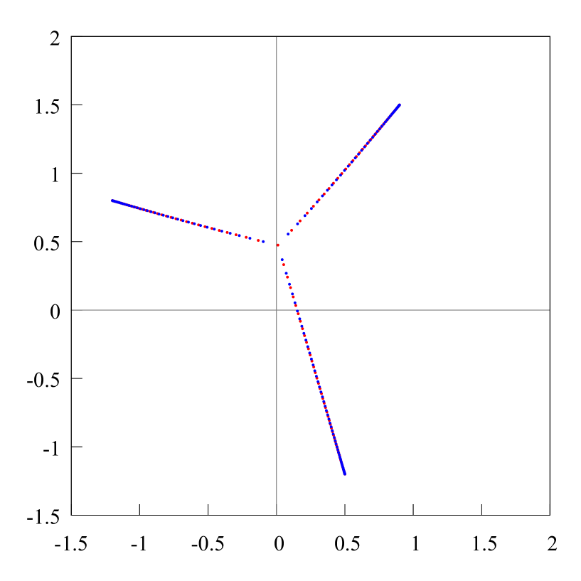
Figure 1. Zeros and poles of the diagonal Padé approximant $[131/131]_{f}$ of the function $f(z)=1/\{(z-(-1.2+i\cdot 0.8))(z-(0.9+i\cdot 1.5))(z-(0.5-i\cdot 1.2))\}^{1/3}$. The zeros and poles of the diagonal Padé approximant $[n/n]_{f}$ are distributed, when $n\to\infty$, according to Stahl’s theorem [62]. When $n=131$ the zeros and poles of the diagonal Padé approximant $[131/131]_{f}$ of the function $f$ are distributed accordingly to the electrostatical model, by E. A. Rakhmanov [52], and they model the Chebotarev-Stahl compact $S_{131}$, which depends on $n$. Froissart doublets are not present when $n=131$.

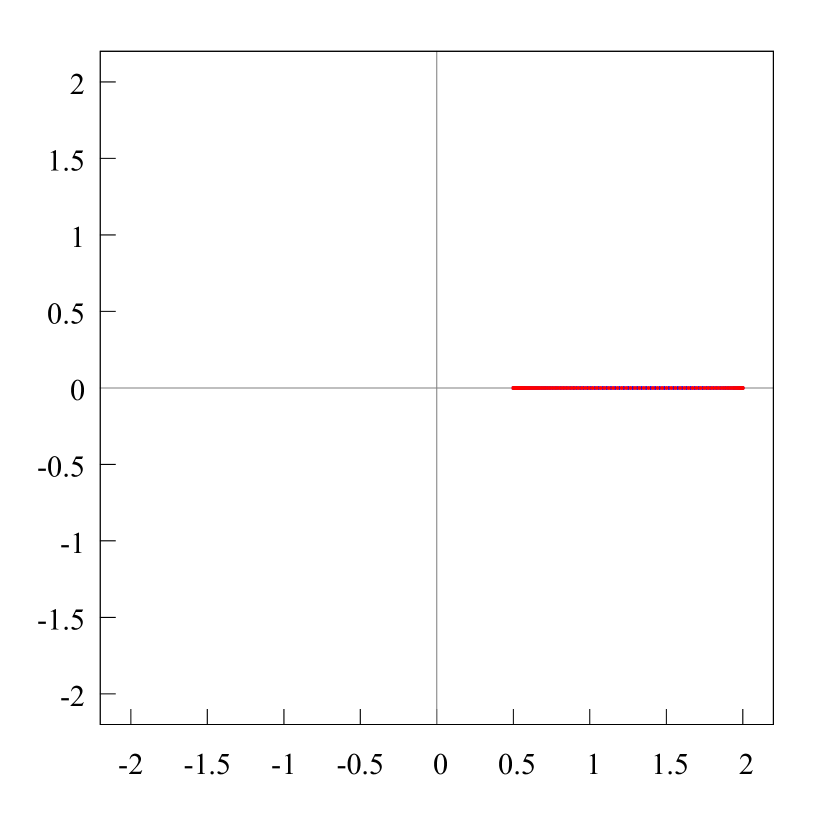
Figure 77. The distribution of zeros and poles of the two-point Padé approximant (at points $z=0$ and $z=\infty$) of the function $f(z)=\sqrt{(z-a)/(z-b)}$, $a=.5$, $b=2$. Here are selected two “same” branches of the function $f$: $f_{0}=\sqrt{(z-.5)/(z-2)}$, $f_{\infty}=\sqrt{(z-.5)/(z-2)}$. The interval $[1/2,2]$ is the Buslaev compact.

For a better exposition of the new numerical results, we state at the beginning some well known facts about the asymptotical behavior of the zeros and poles of the classical Padé approximants, i.e. zeros of the Padé polynomials (see (2)), and also for two-point Padé approximants [20]. These results and their pictures (see fig. 1–11 and fig. 77–79) are needed for the analysis of the numerical results, connected with the behavior of the zeros of the Hermite–Padé polynomials.

2. Main results

The main empirical results obtained in the paper are presented herein.

2.1. Angelesco system

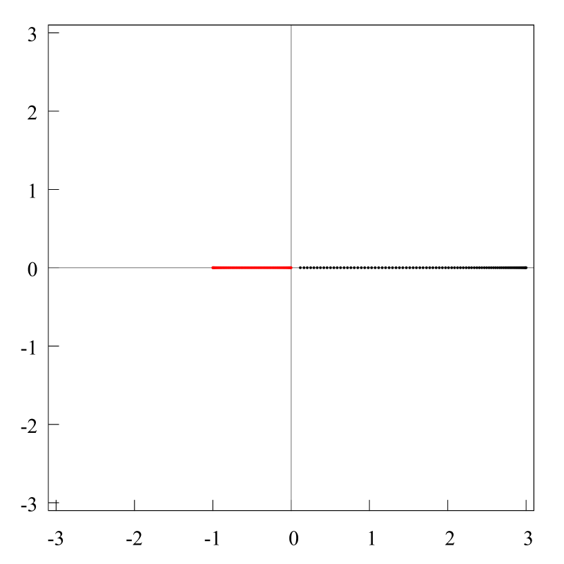
Figure 12. The distribution of the zeros of the Hermite-Padé polynomial $Q_{90,1}$ (red points) and $Q_{90,2}$ (black points) for the set of three functions $[1,f_{1},f_{2}]$, where $f_{1}(z)=\sqrt{(z+1)/z}$, $f_{2}=\sqrt{(z-3)/z}$ (we select such a root branch, that $\sqrt{1\,}=1$). The functions $f_{1},f_{2}$ are of Markov type: $f_{1}(z)=\widehat{\sigma}_{1}(z)$, $f_{2}(z)=\widehat{\sigma}_{2}(z)$, where $\sigma^{\prime}_{1}(x)=\sqrt{(1+x)/(-x)}/\pi$, $x\in(-1,0)$, $\Delta_{1}=\operatorname{supp}{\sigma_{1}}=[-1,0]$, $\sigma^{\prime}_{2}(x)=\sqrt{(3-x)/x}/\pi$, $x\in(0,3)$, $\Delta_{2}=\operatorname{supp}{\sigma_{2}}=[0,3]$. It is known [24], [2], that the zeros of the polynomials $Q_{n,1}$ and $Q_{n,2}$, when taken the limit, are distributed on the support of the equilibrium measures $S_{1}=\lambda_{1}$ and $S_{2}=\lambda_{2}$ and in accordance with their densities $\lambda_{1}^{\prime}(x)$ and $\lambda_{2}^{\prime}(x)$. The figure clearly shows, that $S_{1}=\Delta_{1}$, but $S_{2}=[a_{2}^{*},3]\subsetneq\Delta_{2}$, because $|\Delta_{1}|<|\Delta_{2}|$. The point $a_{2}^{*}\in(0,3)$ is calculated by the formula (12), obtained by V. A. Kalyagin [37] (see also [46], [1]). The density $\lambda_{1}^{\prime}(x)$ behaves, in the neighborhoods of the points $a_{1}$ and $b_{1}$, like $(x-a_{1})^{-1/2}$ and $(b_{1}-x)^{-1/2}$, respectively, and the density $\lambda_{2}^{\prime}(x)$ behaves, in the neighborhood of the point $a_{2}$, like $(x-a^{*}_{1})^{1/2}$ and in the neighborhood of the point $b_{2}$ like $(b_{2}-x)^{-1/2}$.

The first part of the numerical results of the behavior of the Hermite–Padé polynomials for a collection of three functions $[1,f_{1},f_{2}]$ refers to the case when each of the functions $f_{1}$ and $f_{2}$ has a pair of branch points of second order and the sets of the branch points of the functions $f_{1}$ and $f_{2}$ do not intersect. Thus, the pair of functions $f_{1},f_{2}$ forms an Angelesco system (see (3)). About the main properties of the Angelesco system, see [46], also [24]. In [24], the first results of general character about the convergence of the Hermite–Padé approximants of second kind for the collection of functions $[1,f_{1},\dots,f_{m-1}]$, $m\geqslant 3$ were obtained, with the functions $f_{1},\dots,f_{m-1}$ creating an Angelesco system and $f_{j}=\widehat{\sigma}_{j}$ being Markov functions with non-intersecting supports $\Delta_{j}=\operatorname{supp}{\sigma_{j}}$, $j=1,2,\dots,m-1$, along the real axis, and containing a finite number of intervals. In [24], A. A. Gonchar and E. A. Rakhmanov found a new property, which they called pushing of the support of the equilibrium measures (see also [46], [1], [2]). For $m=3$ this method looks as follows. Let the support sets $\Delta_{1},\Delta_{2}$ of the measures $\sigma_{1},\sigma_{2}$ are the non-intersecting closed intervals $\Delta_{1}=[a_{1},b_{1}]$, $\Delta_{2}=[a_{2},b_{2}]$ of different lengths and contained in the real axis; for definiteness we suppose that $|\Delta_{1}|<|\Delta_{2}|$ and that $\Delta_{2}$ be on the right of $\Delta_{1}$. It turns out that in the case when the intervals are close enough, the support $F_{2}\subset\Delta_{2}$ of the equilibrium measure $\lambda_{2}$ is the interval $[a^{*}_{2},b_{2}]$, where $a^{*}_{2}\in(a_{2},b_{2})$ (see (12) and fig. 12). Thus, the equilibrium measures $\lambda_{1},\lambda_{2}$ are absolutely continuous with respect to the normalized linear Lebesgue measure, the density $\lambda_{1}^{\prime}(x)$ behaves, in the neighborhood of the points $a_{1}$ and $b_{1}$, like $(x-a_{1})^{-1/2}$ and $(b_{1}-x)^{-1/2}$, respectively, and the density $\lambda_{2}^{\prime}(x)$ behaves, in the neighborhood of the point $a_{2}$, like $(x-a^{*}_{1})^{1/2}$ and like $(b_{2}-x)^{-1/2}$ around $b_{2}$. Thus, under a specific mutual positions the smaller interval pushes the support of the equilibrium measure inside the larger interval; this does not happen with the support of the equilibrium measure for a smaller interval (see fig. 12). When $[a_{1},b_{1}]=[-a,0]$, $[a_{2},b_{2}]=[0,1]$, where $a\in(0,1)$, the point $a_{2}^{*}$ is calculated by the following formula, found by V. A. Kalyagin [37] (see also [46, p. 5.3, formula (5.3.18)], [1]):

(12) $$a_{2}^{*}=\frac{(1-a)^{3}}{9(a^{2}-a+1)}.$$

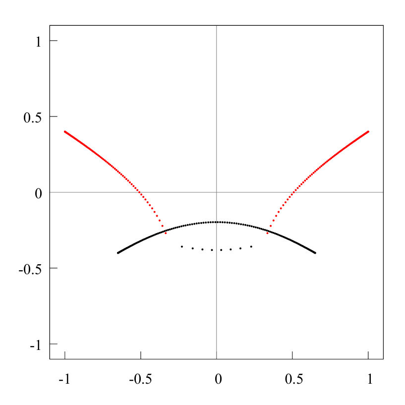
Figure 42. The distribution of the Hermite-Padé polynomials $Q_{180,1}$ (red points), $Q_{180,2}$ (black points) for two functions $f_{1}(z)=1/\sqrt{(z-(-1.0+i\cdot 0.4))(z-(1.0+i\cdot 0.4))}$, $f_{2}(z)=1/\sqrt{(z-(-.65-i\cdot 0.4))(z-(.65-i\cdot 0.4))}$. It is clearly seen, that under this position of the pair of branch points, the two arcs, which are the result of the breaking of the support of the measure $\lambda_{1}$, cross the second compact $F_{2}$. The second compact $F_{2}$ continues to change: from the total set of black points (zeros of the polynomial $Q_{180,2}$) even more points stand out (than before), which form the second component of $F_{2}$. Thus, the forming of the second component of the support of the equilibrium measure $\lambda_{2}$ continues.

The authors have found, by experiments, a new property called mutual pushing of the supports of the equilibrium measures, in the case when the functions $f_{1}$ and $f_{2}$ have a pair of branch points $a_{1},b_{1}\in\mathbb{C}$ and $a_{2},b_{2}\in\mathbb{C}$, $\{a_{1},b_{1}\}\cap\{a_{2},b_{2}\}=\varnothing$, located not on one line, but on two parallel lines, and the intervals $\Delta_{1}=[a_{1},b_{1}]$ and $\Delta_{2}=[a_{2},b_{2}]$ have different lengths, i.e. $|\Delta_{1}|>|\Delta_{2}|$ (see fig. 42).

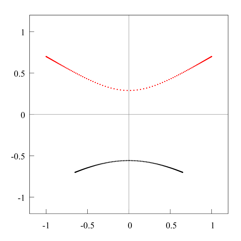
Figure 32. The distribution of the zeros of the Hermite-Padé polynomial $Q_{120,1}$ (red points), $Q_{120,2}$ (black points) in the plane $\mathbb{C}_{z}$ for two functions $f_{1}(z)=1/\sqrt{(z-(-1.0+i\cdot 0.7))(z-(1.0+i\cdot 0.7))}$, $f_{2}(z)=1/\sqrt{(z-(-.65-i\cdot 0.7))(z-(.65-i\cdot 0.7))}$. Since the branch points $a_{1}=-1.0+i\cdot 0.7,b_{1}=1.0+i\cdot 0.7$ and $a_{2}=-0.65+i\cdot 0.7,b_{2}=0.65+i\cdot 0.7$ of the functions are far enough from each other, there is no collision of the supports of the equilibrium measures and the supports $\lambda_{1}$ and $\lambda_{2}$ are two non-intersecting arcs. The measures $\lambda_{1}$ and $\lambda_{2}$ are absolutely continuous with respect to the length of the arc $|dz|$, and their densities $\lambda_{j}^{\prime}$, $j=1,2$, behave, in the neighborhoods of the branch points $a_{j},b_{j}$, like Chebyshev measures, i.e. $\sim|z-a_{j}|^{-1/2}$ and $\sim|z-b_{j}|^{-1/2}$, respectively. It is obvious that the extremal compacts $F_{1}$ and $F_{2}$ are converging to each other, and the zeros of the polynomials $Q_{120,j}$, which are onto $F_{j}$, are diverging from each other and from the branch points $a_{j},b_{j}$, $j=1,2$. The zeros of the polynomial $Q_{120,0}$ (blue points, see fig. 33) create a third extremal compact $F_{0}$, which separates the compacts $F_{1}$ and $F_{2}$.

Fig. 32–33

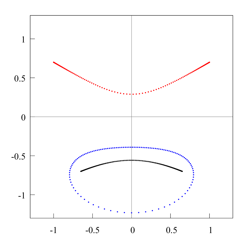
Figure 33. The distribution of the Hermite-Padé polynomials $Q_{120,0}$ (blue points), $Q_{120,1}$ (red points), $Q_{120,2}$ (black points) in the plane $\mathbb{C}_{z}$ for two functions $f_{1}(z)=1/\sqrt{(z-(-1.0+i\cdot 0.7))(z-(1.0+i\cdot 0.7))}$, $f_{2}(z)=1/\sqrt{(z-(-.65-i\cdot 0.7))(z-(.65-i\cdot 0.7))}$. The red points are distributed onto the support of the equilibrium measure $\lambda_{1}$, when taking the limit, accordingly to its density $\lambda^{\prime}_{1}$. The black points are distributed onto the support of the equilibrium measure $\lambda_{2}$, when taking the limit, accordingly to its density $\lambda^{\prime}_{2}$. Same applies for the blue points. Both measures $\lambda_{1}$ and $\lambda_{2}$ are absolutely continuous on the corresponding extremal curves $F_{1}=\operatorname{supp}{\lambda_{1}}$ and $F_{2}=\operatorname{supp}{\lambda_{2}}$ with respect to the length of the arc $ds$, and their densities behave like the Chebyshev measures $|z-a_{j}|^{-1/2},|z-b_{j}|^{-1/2}$, $j=1,2$ around the endpoints of the curves. The blue points (zeros of the polynomial $Q_{120,0}$) separate the red points (zeros of the polynomial $Q_{120,1}$) from the black points (zeros of the polynomial $Q_{120,2}$).

First, when these lines are far enough from each other, there is no collision of the support of the equilibrium measures and the supports of $\lambda_{1}$ and $\lambda_{2}$ are two non-intersecting arcs, respectively, see [46], [48], [2]. The measures $\lambda_{1}$ and $\lambda_{2}$ are absolutely continuous with respect to the length of the arc $|dz|$, and their densities $\lambda_{j}^{\prime}$, $j=1,2$, in the neighborhoods of the branch points $a_{j},b_{j}$, behave like Chebyshev measures, i.e. $\sim|z-a_{j}|^{-1/2}$ and $\sim|z-b_{j}|^{-1/2}$, respectively. This can be seen very well on figure 32, where the red points are the zeros of the Hermite–Padé polynomial $Q_{120,1}$ and the black points are the zeros of $Q_{120,2}$. It is obvious that the extremal compact sets $F_{1}$ and $F_{2}$ are attracted to each other, and the zeros of the polynomials $Q_{120,j}$, which are onto $F_{j}$, are repelled from each other and from the branch points $a_{j},b_{j}$, $j=1,2$. The zeros of the polynomial $Q_{120,0}$ (blue points, see fig. 33) form a third extremal compact $F_{0}$, which separates the compact sets $F_{1}$ and $F_{2}$. The distribution of the zeros of the polynomial $Q_{n,0}$, when $n\to\infty$, is described by the third extremal measure $\lambda_{0}$, $\operatorname{supp}\lambda_{0}=F_{0}$. Thus, the following fact is true (see [60]). Let $U_{n}(z):=\max\{\log|Q_{n,1}(z)|,\log|Q_{n,2}(z)|\}$, $z\in\mathbb{C}$. Then $U_{n}$ is subharmonic in $\mathbb{C}$. Therefore, $U_{n}(z)=-U^{\mu_{n}}(z)$, where $\mu_{n}$ is measure, $|\mu_{n}|\leqslant n$, $U^{\mu_{n}}(z)=-\int\log|z-\zeta|\,d\mu_{n}(\zeta)$ is the logarithmic potential with respect to $\mu_{n}$. For an arbitrary polynomial $Q\in\mathbb{C}[z]$ define the measure

$$\chi(Q)=\sum_{\zeta:Q(\zeta)=0}\delta_{\zeta},$$

which counts the number of zeros of the polynomial $Q$. Then

(13) $$\lim_{n\to\infty}\frac{1}{n}\mu_{n}=\lim_{n\to\infty}\frac{1}{n}\chi(Q_{n,0})=\lambda_{0}$$

(the convergence in (13) is understood as weak convergence of measures).

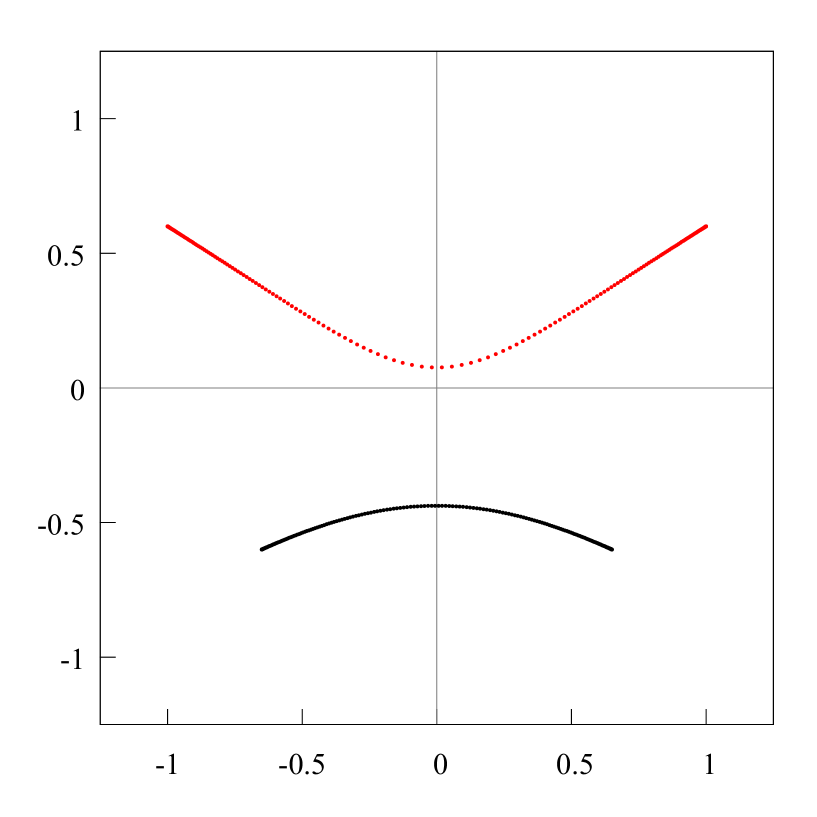
Figure 34. The distribution of the Hermite-Padé polynomials $Q_{180,1}$ (red points), $Q_{180,2}$ (black points) for two functions $f_{1}(z)=1/\sqrt{(z-(-1.0+i\cdot 0.6))(z-(1.0+i\cdot 0.6))}$, $f_{2}(z)=1/\sqrt{(z-(-.65-i\cdot 0.6))(z-(.65-i\cdot 0.6))}$. The branch points have come closer to each other, however they are still far enough from each other and there is no collision of the supports of the equilibrium measures. It is clearly seen, that the upper extremal compact $F_{1}$ has strongly bent towards the lower extremal compact $F_{2}$.

Fig. 34–35

Further convergence of the parallel lines along the imaginary axis leads to the following. While the branch points are far enough from each other, collision of the equilibrium measures does not occur. However, on fig. 34 it is clearly seen, that the upper extremal compact set $F_{1}$ has strongly curved towards the lower extremal compact set $F_{2}$. The third extremal compact set $F_{0}$, as before, separates $F_{1}$ and $F_{2}$.

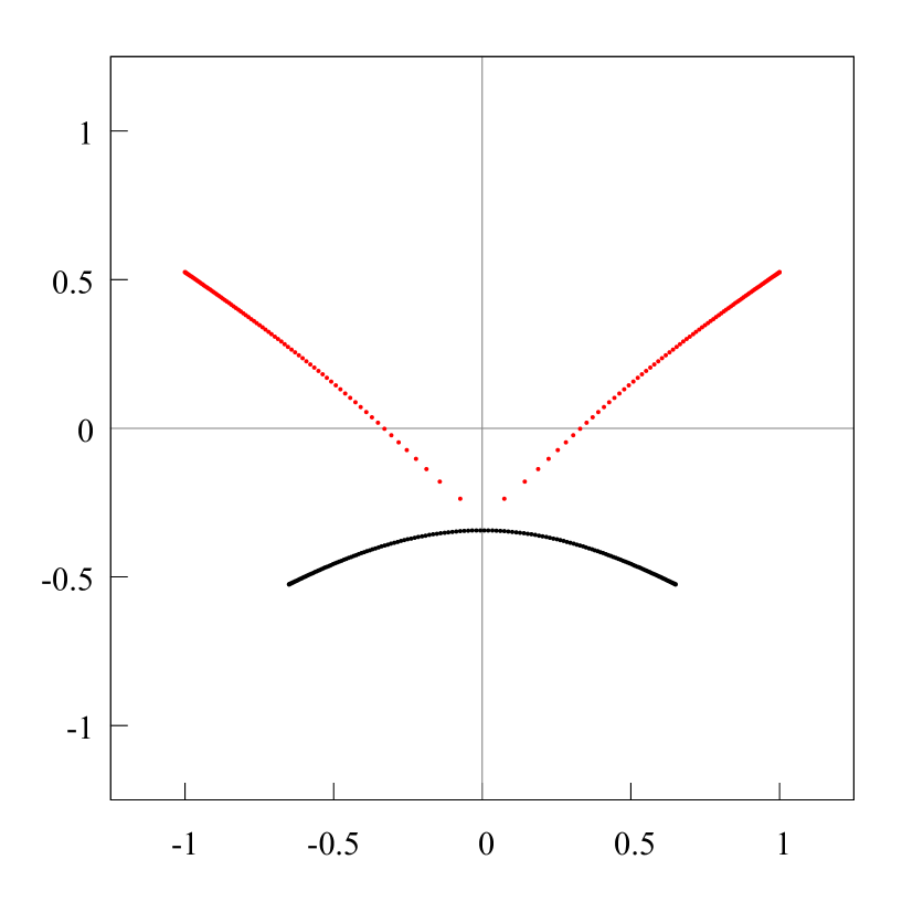
Figure 36. The distribution of the Hermite-Padé polynomials $Q_{180,1}$ (red points), $Q_{180,2}$ (black points) for two functions $f_{1}(z)=1/\sqrt{(z-(-1.0+i\cdot 0.525))(z-(1.0+i\cdot 0.525))}$, $f_{2}(z)=1/\sqrt{(z-(-.65-i\cdot 0.525))(z-(.65-i\cdot 0.525))}$. It is clearly seen, that the upper extremal compact $F_{1}$ has even strongly bent towards the lower extremal compact $F_{2}$. The third extremal compact $F_{0}$, as before, separates $F_{1}$ and $F_{2}$. The support of the equilibrium measure of the upper extremal compact $F_{1}$ starts to break down, while the second compact $F_{2}$ has hardly changed.

Fig. 36–37

Then, under further convergence of the branch points, the upper extremal compact set $F_{1}$ has even strongly curved towards the lower extremal compact set $F_{2}$, the support of the equilibrium measure of the upper compact set $F_{1}$ starts to break down, the second lower compact set almost does not change; see fig. 36. The third extremal compact set $F_{0}$, as before, separates the other two compact sets from each other, but now it touches the second compact set $F_{2}$.

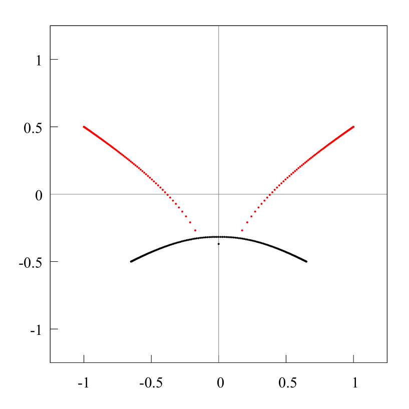
Figure 38. The distribution of the Hermite-Padé polynomials $Q_{180,1}$ (red points), $Q_{180,2}$ (black points) for two functions $f_{1}(z)=1/\sqrt{(z-(-1.0+i\cdot 0.5))(z-(1.0+i\cdot 0.5))}$, $f_{2}(z)=1/\sqrt{(z-(-.65-i\cdot 0.5))(z-(.65-i\cdot 0.5))}$. It is clearly seen, that under this position of the pair of branch points, the support of the equilibrium measure of the upper extremal compact $F_{1}$ breaks down, while the second compact $F_{2}$ has hardly changed. The red points break down the support of the equilibrium measure $\lambda_{1}$ of the compact $F_{1}$ on two arcs.

Fig. 38–39

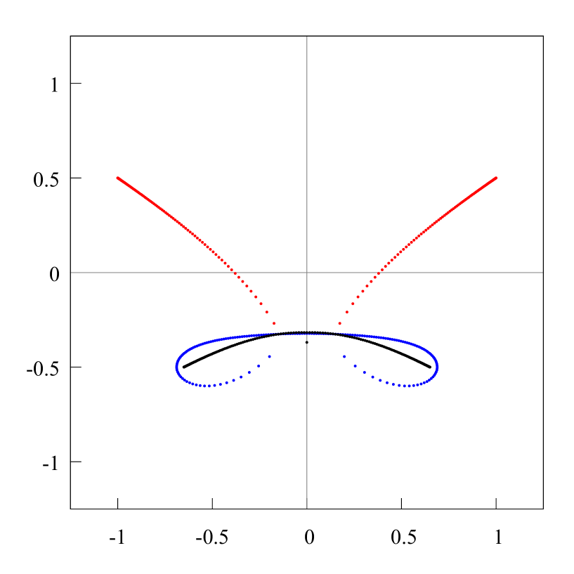
Figure 39. The distribution of the Hermite-Padé polynomials $Q_{180,0}$ (blue points), $Q_{180,1}$ (red points), $Q_{180,2}$ (black points) for two functions $f_{1}(z)=1/\sqrt{(z-(-1.0+i\cdot 0.5))(z-(1.0+i\cdot 0.5))}$, $f_{2}(z)=1/\sqrt{(z-(-.65-i\cdot 0.5))(z-(.65-i\cdot 0.5))}$. It is clearly seen, that under this position of the pair of branch points, the support of the equilibrium measure of the upper extremal compact $F_{1}$ breaks down, while the second compact $F_{2}$ has hardly changed. The third extremal compact $F_{0}$, as before, separates the other two compacts from each other, and touches the second compact $F_{2}$

Finally, under certain relative positions of the pair of branch points, the support of the equilibrium measure of the upper extremal compact $F_{1}$ breaks down, while the second compact set $F_{2}$ has hardly changed, see fig. 38. The third extremal compact set $F_{0}$, as before, separates the other two compact sets from each other, and touches the second compact set $F_{2}$, see fig. 39.

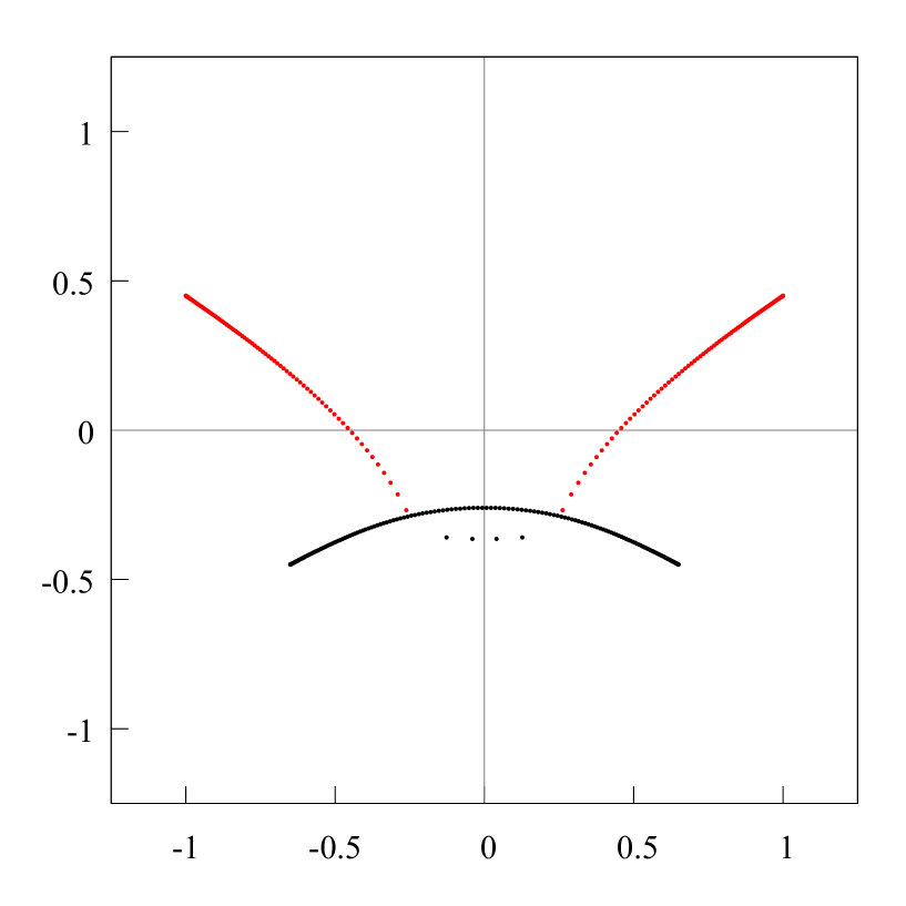
Figure 40. The distribution of the Hermite-Padé polynomials $Q_{180,1}$ (red points), $Q_{180,2}$ (black points) for two functions $f_{1}(z)=1/\sqrt{(z-(-1.0+i\cdot 0.45))(z-(1.0+i\cdot 0.45))}$, $f_{2}(z)=1/\sqrt{(z-(-.65-i\cdot 0.45))(z-(.65-i\cdot 0.45))}$. It is clearly seen, that under this position of the pair of branch points, the two arcs, which are the result of the breaking of the support of the measure $\lambda_{1}$, have reached the second (lower) compact $F_{2}$. The second compact $F_{2}$ has started to change: from the total set of black points (zeros of the polynomial $Q_{180,2}$) several points stand out, which started to form another component. Thus, a second component of the support of the equilibrium measure $\lambda_{2}$ started to form, i.e. the support of the equilibrium measure $\lambda_{2}$ started breaking down on two arcs.

Fig. 40–41

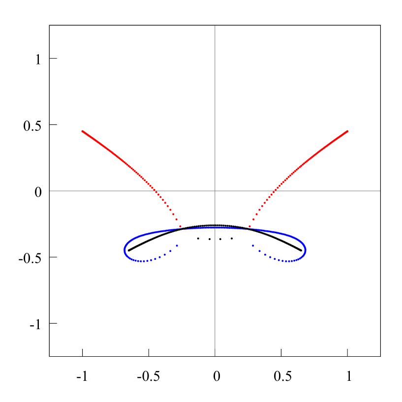
Figure 41. The distribution of the Hermite-Padé polynomials $Q_{180,0}$ (blue points), $Q_{180,1}$ (red points), $Q_{180,2}$ (black points) for two functions $f_{1}(z)=1/\sqrt{(z-(-1.0+i\cdot 0.45))(z-(1.0+i\cdot 0.45))}$, $f_{2}(z)=1/\sqrt{(z-(-.65-i\cdot 0.45))(z-(.65-i\cdot 0.45))}$. It is clearly seen, that under this position of the pair of branch points, the two arcs, which are the result of the breaking of the support of the measure $\lambda_{1}$, have reached the second (lower) compact $F_{2}$. The second compact $F_{2}$ has started to change: from the total set of black points (zeros of the polynomial $Q_{180,2}$) several points stand out, which started to form another component. Thus, a second component of the support of the equilibrium measure $\lambda_{2}$ started to form, i.e. the support of the equilibrium measure $\lambda_{2}$ started breaking down on two arcs. The third extremal compact $F_{0}$, as before, “seeks” to separate the other two compacts from each other, but now each of the compacts $F_{1}$ and $F_{2}$ has by two components. It is clearly seen, that the compact $F_{0}$ now crosses the compact $F_{2}$.

Under further convergence of the pair of branch points, the two arcs, which are the result of the breaking of the support of the measure $\lambda_{1}$, have reached the second (lower) compact set $F_{2}$. The second compact set $F_{2}$ has started to change: from the total set of black points (zeros of the polynomial $Q_{180,2}$) several points stand out, which started to form another component. Thus, a second component of the support of the equilibrium measure $\lambda_{2}$ started to form, i.e. the support of the equilibrium measure $\lambda_{2}$ started breaking down on two arcs; see fig. 40. The third extremal compact set $F_{0}$, as before, “seeks” to separate the other two compact sets from each other, but now each of the compact sets $F_{1}$ and $F_{2}$ has two components. It is clearly seen, that the compact set $F_{0}$ now crosses the compact set $F_{2}$; see fig. 41.

Fig. 42–43

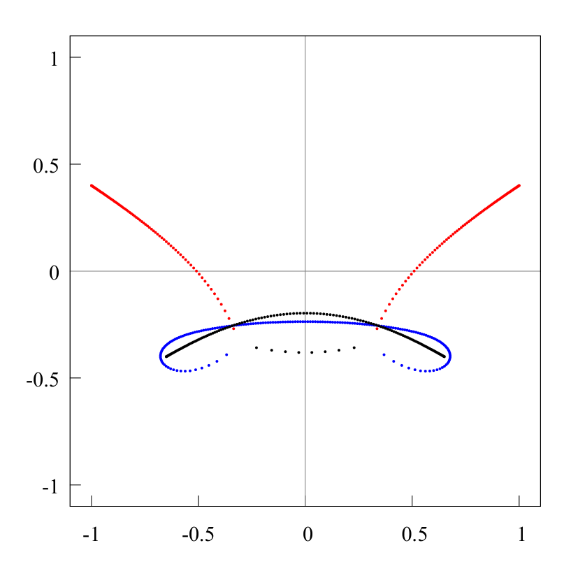
Figure 43. The distribution of the Hermite-Padé polynomials $Q_{180,0}$ (blue points), $Q_{180,1}$ (red points), $Q_{180,2}$ (black points) for two functions $f_{1}(z)=1/\sqrt{(z-(-1.0+i\cdot 0.4))(z-(1.0+i\cdot 0.4))}$, $f_{2}(z)=1/\sqrt{(z-(-.65-i\cdot 0.4))(z-(.65-i\cdot 0.4))}$. It is clearly seen, that under this position of the pair of branch points, the two arcs, which are the result of the breaking of the support of the measure $\lambda_{1}$, cross the second compact $F_{2}$. The second compact $F_{2}$ continues to change: from the total set of black points (zeros of the polynomial $Q_{180,2}$) even more points stand out (than before), which form the second component of $F_{2}$. Thus, the forming of the second component of the support of the equilibrium measure $\lambda_{2}$ continues. The third extremal compact $F_{0}$ crosses the compact $F_{2}$. As before, it “seeks” to separate the other two compacts $F_{1}$ and $F_{2}$ from each other, but now it “fights” with two components. It is clearly seen, that at the junction of the red, black and blue points appear two “equilateral” triangles with multicolored vertexes.

Further, the two arcs, which are the result of the breaking of the support of the measure $\lambda_{1}$, cross the second compact set $F_{2}$. The second compact set $F_{2}$ continues to change: from the total set of black points (zeros of the polynomial $Q_{180,2}$) even more points stand out (than before), which form the second component of $F_{2}$. Thus, the forming of the second component of the support of the equilibrium measure $\lambda_{2}$ continues; see fig. 42. The third extremal compact set $F_{0}$ crosses the compact set $F_{2}$. As before, it “seeks” to separate the other two compact sets $F_{1}$ and $F_{2}$ from each other, but now each of these compact sets has by two components. It is clearly seen, that at the junction of the red, black and blue points appear two equilateral triangles with multicolored vertexes, see fig. 43.

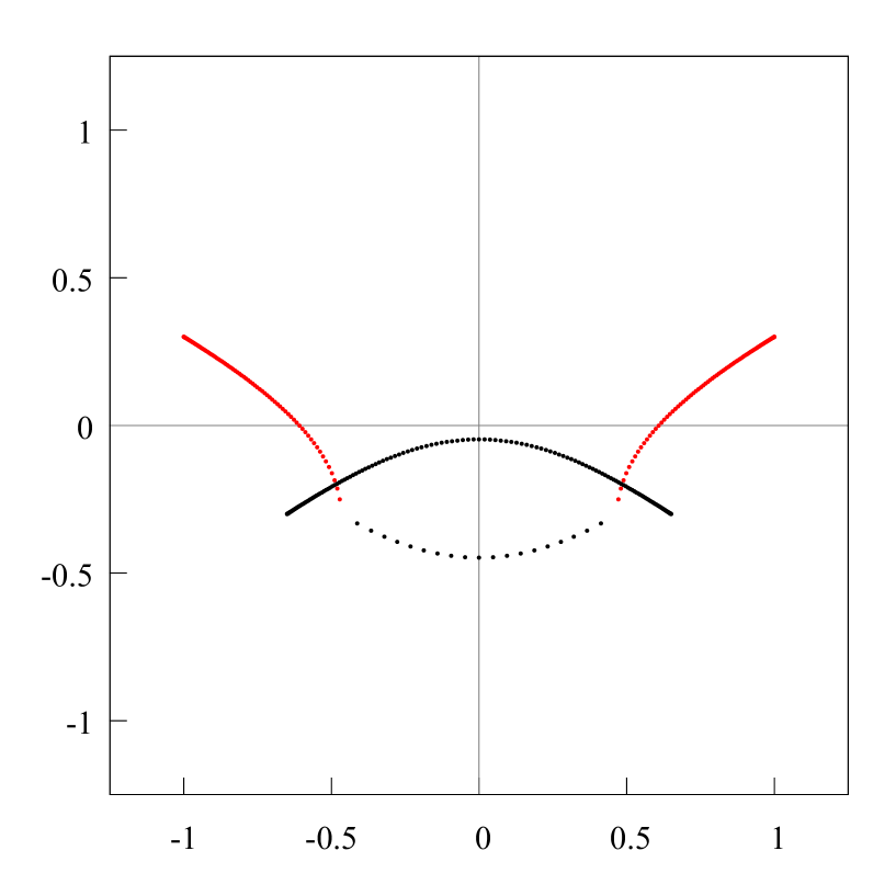
Figure 44. The distribution of the Hermite-Padé polynomials $Q_{180,1}$ (red points), $Q_{180,2}$ (black points) for two functions $f_{1}(z)=1/\sqrt{(z-(-1.0+i\cdot 0.3))(z-(1.0+i\cdot 0.3))}$, $f_{2}(z)=1/\sqrt{(z-(-.65-i\cdot 0.3))(z-(.65-i\cdot 0.3))}$. It is clearly seen, that under this position of the pair of branch points, the two arcs, which are the result of the breaking of the support of the measure $\lambda_{1}$, even further cross the second compact $F_{2}$. The second compact $F_{2}$ continues to change: from the total set of black points (zeros of the polynomial $Q_{180,2}$) even more points stand out (even than before), which form the second component of $F_{2}$. Thus, the forming of the second component of the support of the equilibrium measure $\lambda_{2}$ continues.

Fig. 44–45

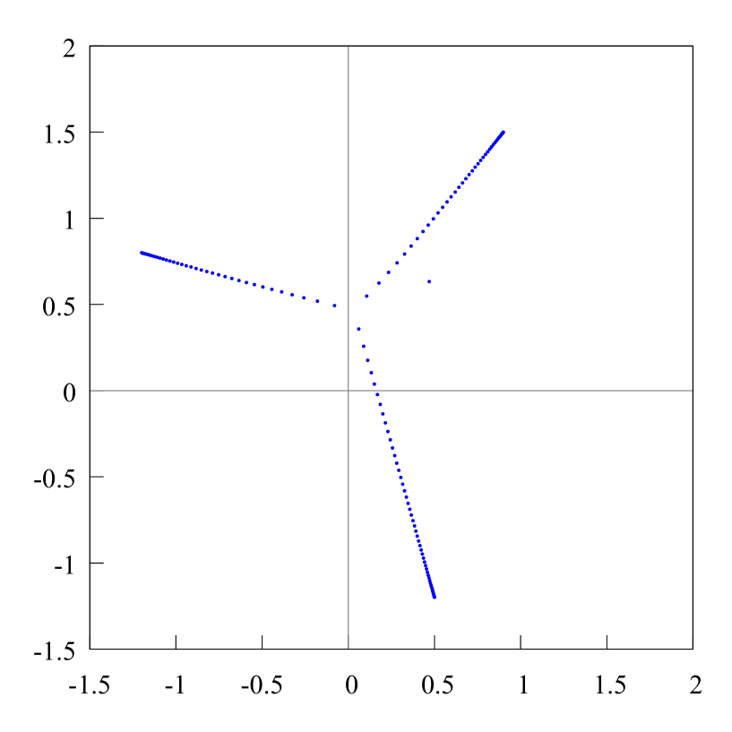
Figure 4. The Chebotarev point should not be approximated by zeros of the Padé approximant $[130/130]_{f}$. There is one spurious zero of the Padé approximant $[130/130]_{f}$, it is accompanied by a spurious pole of the Padé approximant $[130/130]_{f}$ (see fig. 3).

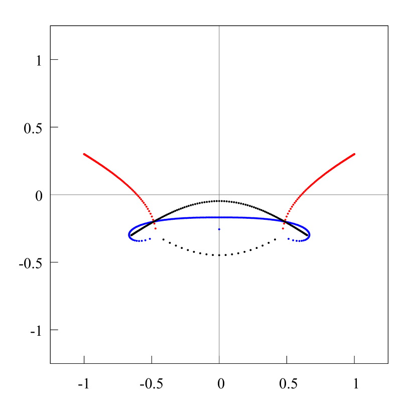
Figure 45. The distribution of the Hermite-Padé polynomials $Q_{180,0}$ (blue points), $Q_{180,1}$ (red points) and $Q_{180,2}$ (black points) for two functions $f_{1}(z)=1/\sqrt{(z-(-1.0+i\cdot 0.3))(z-(1.0+i\cdot 0.3))}$, $f_{2}(z)=1/\sqrt{(z-(-.65-i\cdot 0.3))(z-(.65-i\cdot 0.3))}$. It is clearly seen, that under this position of the pair of branch points, the two arcs, which are the result of the breaking of the support of the measure $\lambda_{1}$, even further cross the second compact $F_{2}$. The second compact $F_{2}$ continues to change: from the total set of black points (zeros of the polynomial $Q_{180,2}$) even more points stand out (even than before), which form the second component of $F_{2}$. Thus, the forming of the second component of the support of the equilibrium measure $\lambda_{2}$ continues. It is clearly seen, that at the junction of the red, black and blue points appear two “equilateral” triangles with multicolored vertexes. By analogy with classical Padé approximants and two-point Padé approximants (see fig. 4 and 78) it is natural to assume, that the center of each triangle has a Chebotarev point $v_{1}$, $v_{2}$ with zero density. At the branch points $a_{j},b_{j}$ the density of the measures $\lambda_{1}$ and $\lambda_{2}$ are proportional to $|z-a_{j}|^{-1/2},|z-b_{j}|^{-1/2}$, $j=1,2$, respectively. There is a Froissart singlet (blue) on the imaginary axis.

The two arcs, which are the result of the breaking of the support of the measure $\lambda_{1}$, even further cross the second compact set $F_{2}$. The second compact set $F_{2}$ continues to change: from the total set of black points (zeros of the polynomial $Q_{180,2}$) even more points stand out (even than before), which form the second component of $F_{2}$. Thus, the forming of the second component of the support of the equilibrium measure $\lambda_{2}$ continues. It is clearly seen, that at the junction of the red, black and blue points appear two equilateral triangles with multicolored vertexes. By analogy with classical Padé approximants and two-point Padé approximants (see fig. 4 and 78), it is natural to assume, that the center of each triangle has a Chebotarev point $v_{1}$, $v_{2}$ with zero density. At the branch points $a_{j},b_{j}$ the density of the measures $\lambda_{1}$ and $\lambda_{2}$ are proportional to $|z-a_{j}|^{-1/2},|z-b_{j}|^{-1/2}$, $j=1,2$, respectively. There is a Froissart singlet (blue) on the imaginary axis; see fig. 45, 44.

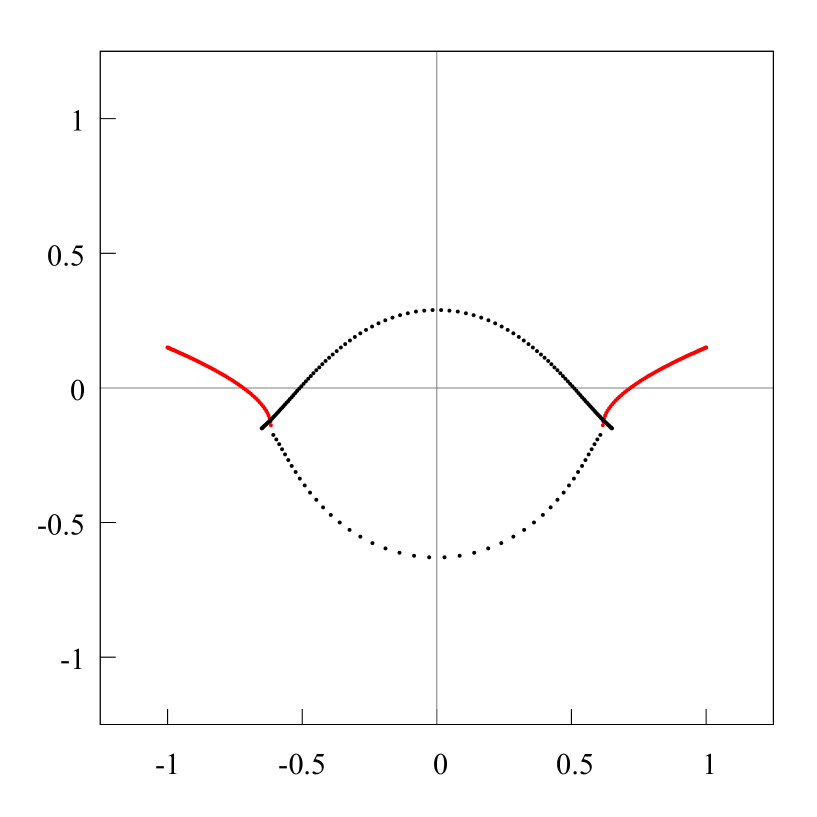
Figure 46. The distribution of the Hermite-Padé polynomials $Q_{180,1}$ (red points), $Q_{180,2}$ (black points) for two functions $f_{1}(z)=1/\sqrt{(z-(-1.0+i\cdot 0.15))(z-(1.0+i\cdot 0.15))}$, $f_{2}(z)=1/\sqrt{(z-(-.65-i\cdot 0.15))(z-(.65-i\cdot 0.15))}$. It is clearly seen, that under this position of the pair of branch points, the support $F_{2}$ of the equilibrium measure $\lambda_{2}$ is separated on two practically equivalent arcs. However, according to the distribution of the zeros of the polynomial $Q_{180,2}$, the density $\lambda_{2}^{\prime}$ of the equilibrium measures of each arc must be different. On the upper arc it behaves like a Chebyshev measure, that is at the end points $a_{2},b_{2}$ the density is proportional to $|z-a_{2}|^{-1/2}$ and $|z-b_{2}|^{-1/2}$, respectively. The end points of the lower arc $v_{1},v_{2}$ are the Chebotarev points and their density is proportional to $|z-v_{1}|^{1/2}$ and $|z-v_{2}|^{1/2}$.

Fig. 46–47

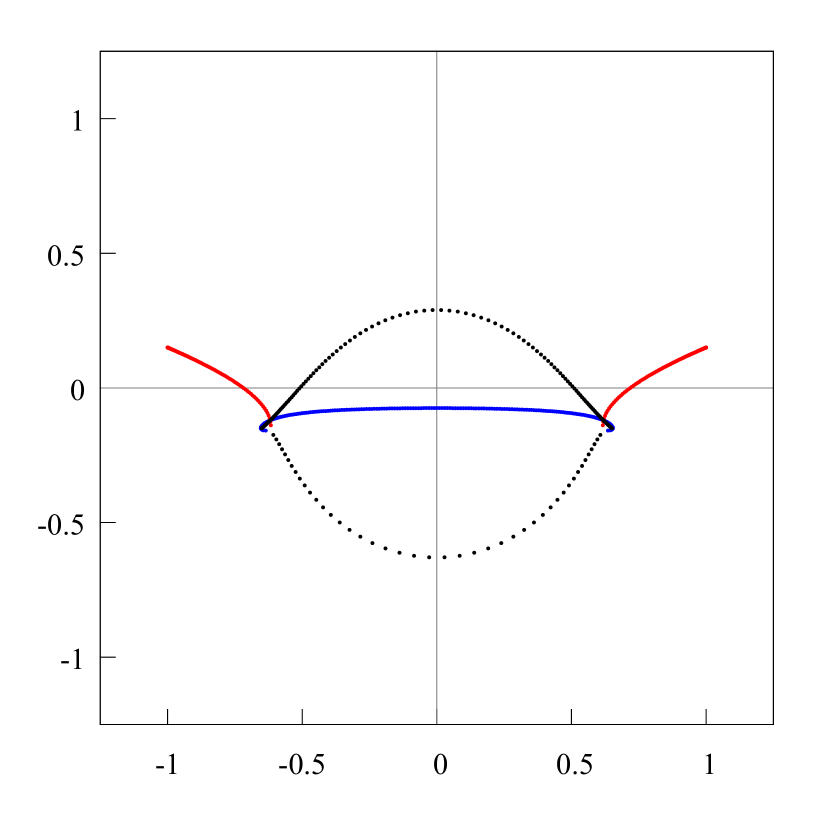
Figure 47. The distribution of the Hermite-Padé polynomials $Q_{180,0}$ (blue points), $Q_{180,1}$ (red points), $Q_{180,2}$ (black points) for two functions $f_{1}(z)=1/\sqrt{(z-(-1.0+i\cdot 0.15))(z-(1.0+i\cdot 0.15))}$, $f_{2}(z)=1/\sqrt{(z-(-.65-i\cdot 0.15))(z-(.65-i\cdot 0.15))}$. It is clearly seen, that under this position of the pair of branch points, the support $F_{2}$ of the equilibrium measure $\lambda_{2}$ is separated on two practically equivalent arcs. The branch points $a_{2},b_{2}$ are on the upper arc, the end points of the lower arc $v_{1},v_{2}$ are the Chebotarev points and their density is proportional to $|z-v_{1}|^{1/2}$ and $|z-v_{2}|^{1/2}$. At the junction of the red, black and blue points appeared two “equilateral” triangles with multicolored vertexes, and the center of each has a Chebotarev point $v_{1},v_{2}$.

Finally, under certain relative positions of the pairs of branch points, the support $F_{2}$ of the equilibrium measure $\lambda_{2}$ is separated on two practically equivalent arcs. However, according to the distribution of the zeros of the polynomial $Q_{180,2}$, the density $\lambda_{2}^{\prime}$ of the equilibrium measures of each arc must be different. On the upper arc it behaves like a Chebyshev measure, that is at the end points $a_{2},b_{2}$ the density is proportional to $|z-a_{2}|^{-1/2}$ and $|z-b_{2}|^{-1/2}$, respectively. The end points of the lower arc $v_{1},v_{2}$ are the Chebotarev points and their density is proportional to $|z-v_{1}|^{1/2}$ and $|z-v_{2}|^{1/2}$; see fig. 46. At the junction of the red, black and blue points appeared two equilateral triangles with multicolored vertexes, and the center of each has a Chebotarev point $v_{1},v_{2}$; see fig. 47.

2.2. Nikishin system

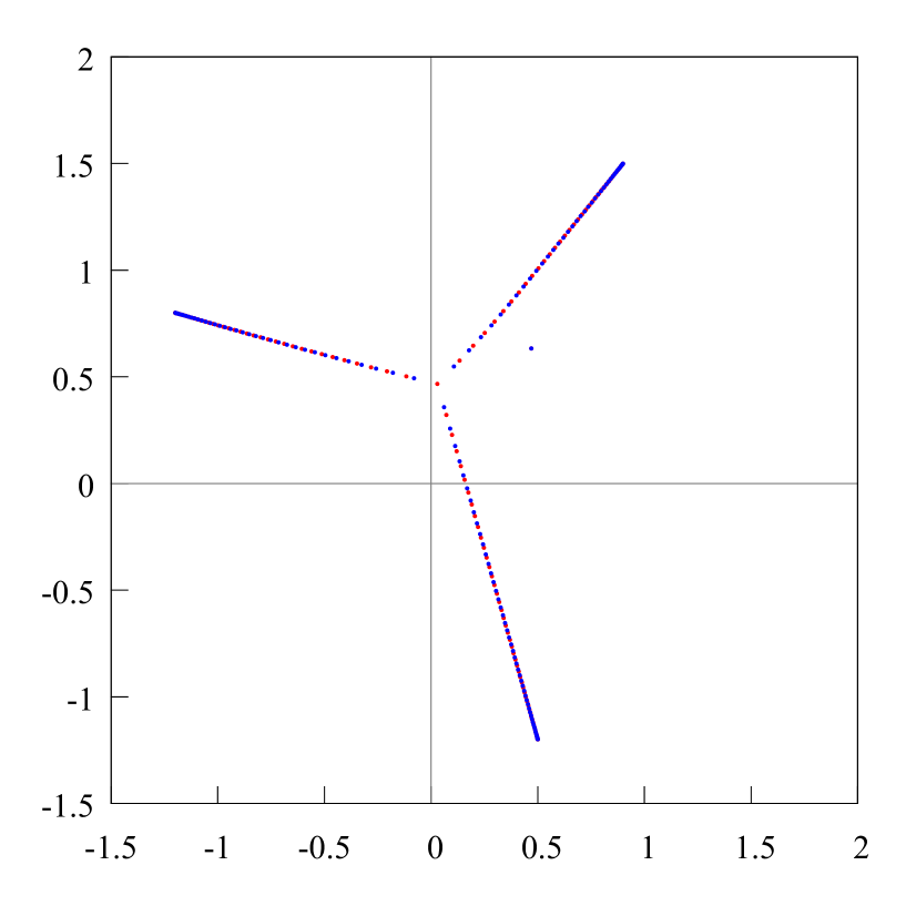
Figure 2. Zeros and poles of the diagonal Padé approximant $[130/130]_{f}$ of the function $f(z)=1/\{(z-(-1.2+i\cdot 0.8i))(z-(0.9+i\cdot 1.5))(z-(0.5-i\cdot 1.2))\}^{1/3}$, distributed accordingly to the electrostatical model by E. A. Rakhmanov [52]. There is a Froissart doublet when $n=130$ (see also fig. 3 and fig. 4). Since the genus of the Riemann surface is $1$, there might be at most one Froissart doublet. In full compliance with the Rakhmanov model [52], the Froissart doublet “attracts” the Stahl $S$-compact $S_{130}$, comp. fig. 1.

In the theory of Padé approximants it is well known the property called “Froissart doublets”, which was experimentally found (see [16], [30], [29]) and means that in the maximal domain of holomorphy $D=D(f)$ of the multi-valued function $f$ for some $n\in\Lambda$, $\Lambda\subset\mathbb{N}$ is an infinite sequence, are positioned pairs of zero-pole of a diagonal Padé approximant (that is, different from each other zeros of the Padé polynomials $P_{n,0},P_{n,1}$, see fig. 2–11). For every fixed $n\in\Lambda$, these points are different from each other, the pole is not dependent of any singularity of the original function, the zero and the pole are infinitely close to each other when $n\to\infty$, that is they are asymptotically “canceled out”. In other words, the residue of the Padé approximant at such a pole converges to zero when $n\to\infty$. Because such poles do not correspond to the singularities of the original function, sometimes they are called “spurious” poles and zeros or “defects” of the diagonal Padé approximant. In a typical case these poles and zeros are dense on the Riemann surface $\overline{\mathbb{C}}$ when $n\to\infty$, $n\in\Lambda$ (see [61], [64], [66], [68], [70]). Thus they are sometimes called wondering poles and zeros or floating poles and zeros. For an arbitrary algebraic function $f$ the number of these pairs depends mainly on the genus of the corresponding Riemann surface, and also of the number of zeros of the functions $\Delta{f}(\zeta)=(f^{+}-f^{-})(\zeta)$, $\zeta\in{S}$, on the Stahl compact set $S=S(f)$. It is shown in [68], that the appearance of the Froissart doublets is due to points of an “incorrect” interpolation of the diagonal Padé approximants $[n/n]_{f}:=-P_{n,0}/P_{n,1}$ in the Stahl domain $D(f)=\overline{\mathbb{C}}\setminus{S}$ with another branch $\widetilde{f}$ of the original function $f$ when $n\in\Lambda$. Namely, the existence of Froissart doublets does not allow uniform convergence of the Padé approximants in the Stahl domain (for details see below).

The second part of the numerical experiments are in the case, when the sets of singularity points for the two functions $f_{1}$ and $f_{2}$ intersect each other. Specifically, we select a collection of three functions $[1,f,f^{2}]$, where the function $f$ is of the type (4) and thus, the pair of functions $f,f^{2}$ forms a Nikishin system (see [5], [49]). In this case another new property has been found. Namely, the appearance of triple zeros (Froissart triplets, see below), i.e. zeros of the Hermite–Padé polynomials $Q_{n,0},Q_{n,1},Q_{n,2}$, which are very close to each other, but still have different values. These zeros are in the domain of holomorphy of the functions $f,f^{2}$, do not correspond to either zeros, nor singularities of these function, for each $n$ they are practically identical to each other and with the transfer from $n$ to $n+1$ they shifted in the complex plane as one unit. It is appropriate to compare these triplets with the very well known Froissart doublets for classical Padé polynomials (see [23], also [16], [30], [31], [29], [33], [18], [17], [62], [19]). Froissart doublets are sometimes called “defects” [16, Chapter 2, § 2.2], and also spurious or wondering (floating) zeros and poles of the Padé approximant [16], [22] (see also [68]).

It is considered that the existence of such zeros and poles of the Padé approximant does not allow uniform convergence of the Padé approximant. Because such zeros and poles are infinitely close to each other asymptotically, then when the limit is taken, they are practically “canceled out”. For some classes of hyperelliptic functions $f$, which allow the representation $f=\widehat{\sigma}$, where the support $S_{\sigma}=\bigsqcup\limits_{j=1}^{2g+2}[e_{2j-1},e_{2j}]\subset\mathbb{R}$ of the measure $\sigma$ consists of finite number of non-intersecting intervals, it was shown [65], [69], [9] that the movement of such poles is subject to certain regularity. Namely, the corresponding divisor of the Nuttall $\Psi$ function (see [65], [69], [9]) moves along a Riemann surface $\mathfrak{R}_{2}$ with two sheets of genus $g\geqslant 1$ and is subject to the general Dubrovin system:

(14) $$\dot{z}_{k}=-\frac{2w(\mathbf{z}_{k})}{\prod\limits_{j\neq k}(z_{k}-z_{j})}\int_{e_{2g+2}}^{\infty}\frac{\prod\limits_{j\neq k}(x-z_{j})}{w(x)}\,dx,\qquad k=1,\dots,g,$$

where $\dot{z}_{k}=dz_{k}/dt$, $e_{2g+2}$ is the rightmost point of the support $S_{\sigma}=\bigsqcup\limits_{j=1}^{2g+2}[e_{2j-1},e_{2j}]\subset\mathbb{R}$ of the measure $\sigma$ (it is supposed, that the support of the measure $\sigma$ has $g\geqslant 1$ gaps, the endpoints of the intervals of the support are numbered according to the ascending values, and the path of integration in (14) is part of the real axis $[e_{2g+2},+\infty)$; for details about the notations see [66]). The points $\mathbf{z}_{1}(t),\dots,\mathbf{z}_{g}(t)$, $t\in\mathbb{R}_{+}$, are on the corresponding hyperelliptic Riemann surface $\mathfrak{R}_{2}$ of genus $g$. If $r$ is a real-valued rational function, which has poles only outside $\widehat{S}_{\sigma}$, then for ${f}=\widehat{\sigma}+r$ we have: $[n/n]_{{f}}\to{f}$ in the spherical metric locally uniformly in $\overline{\mathbb{C}}\setminus\widehat{S}_{\sigma}$ ($[n/n]_{f}:=-P_{n,1}/P_{n,0}$); thus, each pole $r$ attracts exactly the number of poles of $[n/n]_{{f}}$, as its multiplicity (see [28]). In this case the movement of the poles and the points of interpolation of the Padé approximants $[n/n]_{{f}}$, which are in the gaps between intervals, are subject to the system (14).

The fact, that such poles of the Padé approximants form a pair with the zeros that are near them and in this pair they are asymptotically close to each other and when taking the limit are canceled out, has led some authors to believe that their appearance is random and is not connected with the nature of the original function $f$. Such an approach to this property reflected on the respective terminology: such zeros and poles of the approximant began to be called “spurious”. Their appearance, when using Padé approximants, was considered especially negatively in [16], [17], [63], therefore when $n\in\Lambda$ the Padé approximants $[n/n]_{f}$ themselves sometimes were thought to be defective or entirely excluded from the research [16, Chapter 2, § 2.3] or was proposed of using the so-called “purification” of the spurious poles [61].

In [32] Dumas researched the problem of the asymptotical behavior of the sequence $\{[n/n]_{d}\}_{n\in\mathbb{N}}$ for elliptic functions of the special form

(15) $$d(z)=\sqrt{(z-e_{1})\dotsb(z-e_{4})}-z^{2}+\left(e_{1}+\dotsb+e_{4}\right)z/2,$$

where the points $e_{1},\dots,e_{4}\in\mathbb{C}$ are pairwise different and such root branch is selected, that the main member of which, in a neighborhood of the point $z=\infty$, is equal to $z^{2}$; thus $d\in\mathscr{H}(\infty)$. Particularly, Dumas has shown that in “general position” the set of poles of the Padé approximants $[n/n]_{d}$ is dense in $\overline{\mathbb{C}}$.

In [67] the result of Dumas has been extended to some classes of elliptical functions. It was found [68, § 1, par .2] the following property: for each $n$, from some subsequence $\Lambda$, always exists a point $\beta=\beta_{n}\in{D}=\overline{\mathbb{C}}\setminus{S}$, for which $[n/n]_{d}(\beta_{n})=\widetilde{d}(\beta_{n})$, where $\widetilde{d}(z)=-\sqrt{(z-e_{1})\dotsb(z-e_{4})}-z^{2}+(e_{1}+\dotsb+e_{4})z/2$ is another branch of the elliptical function (15) in $D$. Thus, for each $n$, from some subsequence $\Lambda$, the diagonal Padé approximants $[n/n]_{d}$ interpolate at some point from the domain $D$ another branch $\widetilde{d}$ of the function $d$. In the case of general position, such points of the “incorrect” interpolation $\{\beta_{n}\}_{n\in\Lambda}$ are dense in $\overline{\mathbb{C}}$. In [68] were obtained much more general results in this direction.

In the work of E. A. Rakhmanov [52] was obtained an electrostatic interpretation of the poles of the diagonal Padé approximant $[n/n]_{f}$ for some algebraic functions $f$ for each fixed $n$. In this framework, the spurious poles play a special role: they should be considered a part of the “external field”.

2.3.

In the present work, experimentally was obtained a new property for the Nikishin system $f_{1}=f,f_{2}=f^{2}$, where

(16) $$f(z)=(z^{2}-1)^{1/4}(z-a)^{-1/2},\quad\text{where}\quad f(\infty)=1,\quad a\notin\mathbb{R},$$

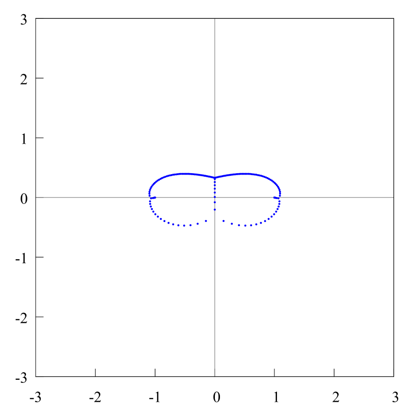
Figure 58. The distribution of the zeros of the Hermite-Padé polynomials $Q_{n,0}$ (blue points), $n=121,\dots,130$, in the plane $\mathbb{C}_{z}$ for a set of three functions $[1,f,f^{2}]$, where $f(z)=(1-z^{2})^{1/4}(1-i\sqrt{3}\cdot 1.6z)^{-1/2}$. There are no Froissart zeros when $n=165$.

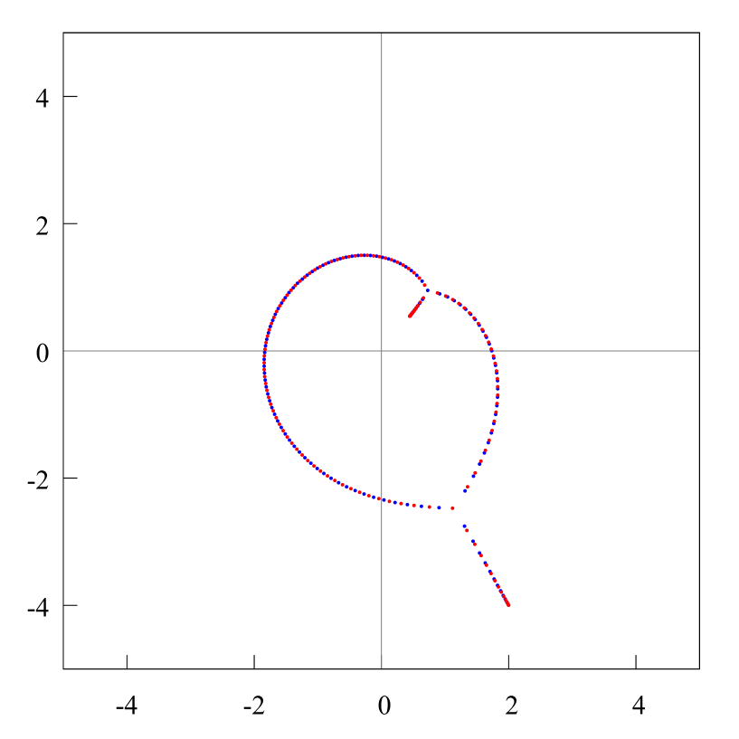
Figure 79. The distribution of zeros and poles of the two-point Padé approximant of order $[120/120]$ of the function $f(z)=(z-a_{1})^{\alpha}(z-a_{2})^{-\alpha}$, $\alpha=1/4$, $a_{1}=0.9-i\cdot 1.1$ ,$a_{2}=0.1+i\cdot 0.2$, when two “quite different” branches are selected, $f_{0}=\sqrt[4]{(z-a_{1})/(z-a_{2})}$, $f_{\infty}=-\sqrt[4]{(z-a_{1})/(z-a_{2})}$. The zeros (blue points) and the poles (red points) create a Buslaev compact.

which is connected with the behavior of the zeros of the Hermite–Padé polynomials of first kind. Namely, there appear, for some $n\in\Lambda=\Lambda(f)$, single spurious zeros of the Hermite–Padé polynomials, and also triple spurious zeros of the Hermite–Padé polynomials. Under “spurious” zeros of the Hermite–Padé polynomials we understand such zeros that, first, are different from each other (they cannot be canceled out), second, do not correspond to either zeros, nor singularities of the original function, and third, significantly change their location, when we transfer from $n$ to $n+1$ (sometimes they may disappear). By analogue with Padé polynomials, it is naturally to call such zeros Froissart singlets and Froissart triplets. It is natural to assume the same as for Padé approximants, in the “typical” case (i.e. for the branch points $a$, which are in “general position”, that is $a\notin i\mathbb{R}$, see (16)) these spurious zeros (singlets and triplets) of the Hermite–Padé polynomials are dense only in “their” domain, which is the difference from Padé approximants. From the numerical experiments it follows that (see fig. 58, 59, 76) the zeros of the polynomials $Q_{n,0}$ and $Q_{n,2}$ of the functions of type (16) when $a=i\cdot 1.6$ have the same limiting distribution, the corresponding boundary compact set $F_{2}$ separates the Riemann surface into three domains, two of which have an internal boundary arc. Thus, they have the same structure (see fig. 79) as in the theorem of Buslaev [20], [21] for two-point Padé approximants. Remark that, the single zeros of the polynomial $Q_{n,2}$ at the point $z\approx a$ corresponds to a simple pole of the function $f^{2}$ at the point $z=a$. The corresponding compact set $F_{2}$ has four Chebotarev’s points (three of which have zero density and one has infinite density) for the equilibrium measure, which corresponds to the limiting distribution of the zeros of the Hermite–Padé polynomials $Q_{n,0},Q_{n,2}$. It is clear, that the distribution of the zeros of the Hermite–Padé polynomials $Q_{n,0}$ and $Q_{n,2}$ must be equivalent, since with the mapping $f\mapsto 1/f$ the type of the singularity of the original function stays the same (see (16)).

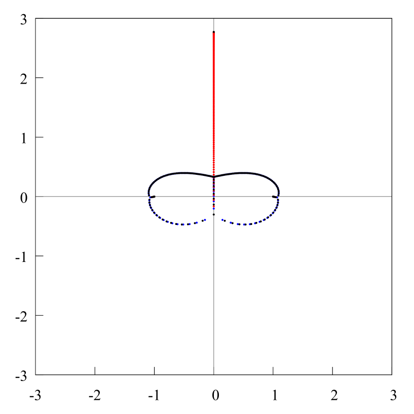
Figure 56. The distribution of the zeros of the Hermite-Padé polynomials $Q_{165,0}$ (blue points), $Q_{165,1}$ (red points), $Q_{165,2}$ (black points) when $n=165$ for a set of three functions $[1,f,f^{2}]$, where $f(z)=(1-z^{2})^{1/4}(1-i\sqrt{3}\cdot 1.6z)^{-1/2}$. The Riemann sphere is decomposed into 3 domains by the zeros of the Hermite-Padé polynomials, one of them contains the infinity point, while the other two are symmetrical with respect to the imaginary axis. There are no Froissart zeros when $n=165$.

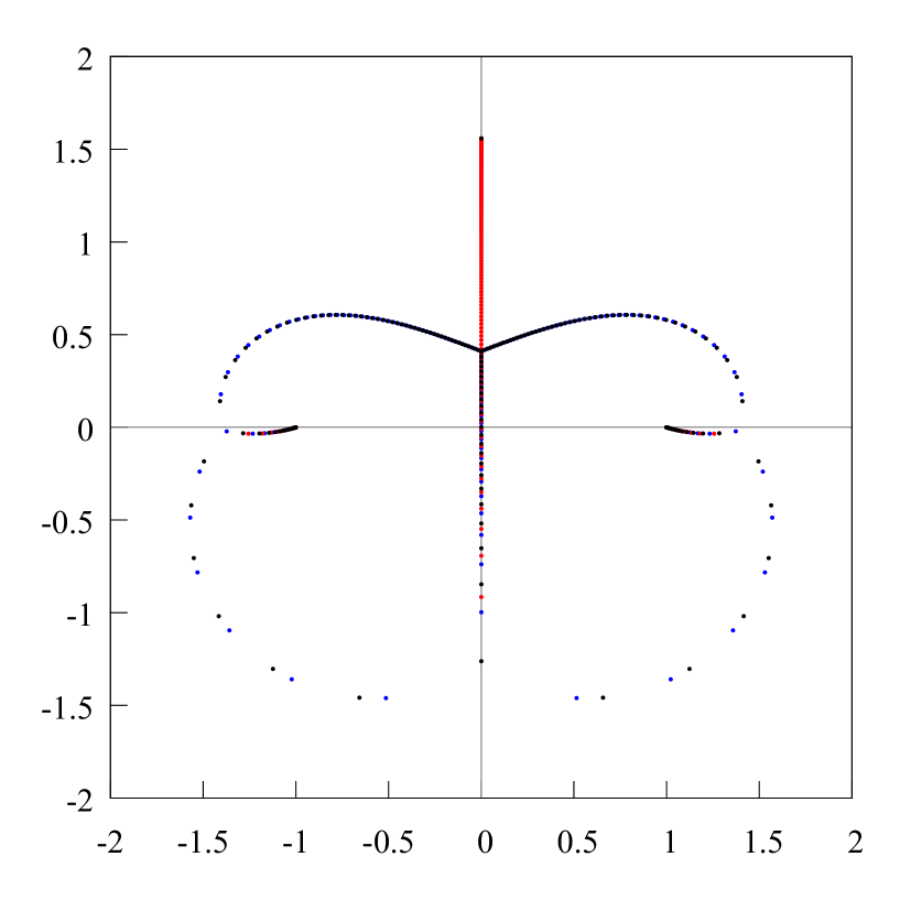
Figure 72. The distribution of the zeros of the Hermite-Padé polynomials $Q_{187,0}$ (blue points), $Q_{187,1}$ (red points), $Q_{187,2}$ (black points) when $n=187$ for a set of three functions $[1,f,f^{2}]$, where $f(z)=(1-z^{2})^{1/4}(1-i\sqrt{3}\cdot 0.9z)^{-1/2}$. The Riemann sphere is decomposed into 3 domains by the zeros of the Hermite-Padé polynomials, one of them contains the infinity point, while the other two are symmetrical with respect to the imaginary axis. There are no Froissart points when $n=187$.

The limiting distribution of the zeros of the polynomial $Q_{n,1}$ must be different. That is, it must correspond to the second compact set $F_{1}$ (see fig. 56, 57 and fig. 72–75). If now we substitute $F:=F_{1}\cup F_{2}$, $F_{1}\cap F_{2}\neq\varnothing$, then the complement $\overline{\mathbb{C}}\setminus{F}$, as before, consists if three domains, but now each of these domains has an internal boundary arc (see fig. 79). Thus, $\overline{\mathbb{C}}=F\sqcup D_{1}\sqcup D_{2}\sqcup D_{3}$. Since the pair $f,f^{2}$ forms a Nikishin system, then by the analogy with [50], [51], [38], [71], we can associate with the collection of functions $[1,f,f^{2}]$ a Nuttall condenser. After then by the analogue with [51], we can to describe in terms of the condenser the limiting distribution of the zeros of the Hermite–Padé polynomials $Q_{n,0},Q_{n,1},Q_{n,2}$ and the corresponding Riemann surface with the canonical (in Nuttall’s sense) partition into three sheets. After that, with the help of this Riemann surface, it might be possible to find strong asymptotics for the Hermite–Padé polynomials. The question about how exactly to do this stays open; a heuristical method for solving this problem for functions of the type $f(z)=(z-a_{1})^{\alpha_{1}}(z-a_{2})^{\alpha_{2}}(z-a_{3})^{\alpha_{3}}$, $\alpha_{1}+\alpha_{2}+\alpha_{3}=0$, $2\alpha_{j}\in\mathbb{C}\setminus\mathbb{Z}$, is proposed in [71].

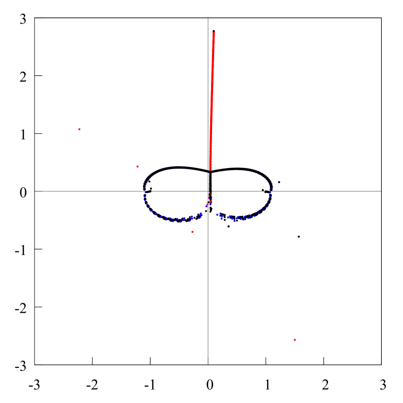
Figure 64. The distribution of the zeros of the Hermite-Padé polynomials $Q_{n,0}$ (blue points), $Q_{n,1}$ (red points), $Q_{n,2}$ (black points), $n=121,\dots,130$, for a set of three functions $[1,f,f^{2}]$, where $f$ is a “perturbed” function: $f(z)=(1-z^{2})^{1/4}(1-(0.1+i\sqrt{3}\cdot 1.6)z)^{-1/2}$. The Riemann sphere is decomposed into 3 domains by the zeros of the Hermite-Padé polynomials, one of them contains the infinity point, while the other two are symmetrical with respect to the imaginary axis. There is a pair of Froissart triplets inside these two domans for some $n\in\{121,\dots,130\}$, there is a pair of Froissart singlets in the complementary domains for some $n\in\{121,\dots,130\}$, there is one Froissart doublet on the negative part of the imaginary axis. This follows from the analysis of the next figures 65, 66 and 67. It is clearly seen, that the picture of the distribution of the zeros is entirely the same compared to the unperturbed case.

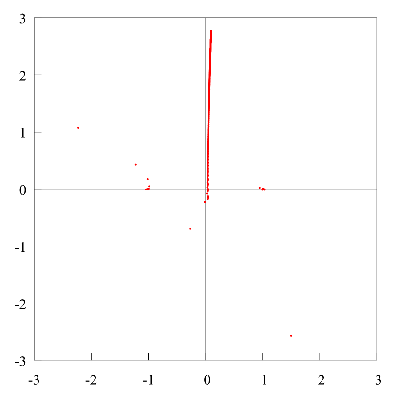
Figure 65. The distribution of the zeros of the Hermite-Padé polynomials $Q_{n,1}$ (red points), $n=121,\dots,130$, for a set of three functions $[1,f,f^{2}]$, where $f$ is a “perturbed” function: $f(z)=(1-z^{2})^{1/4}(1-(0.1+i\sqrt{3}\cdot 1.6)z)^{-1/2}$.

Figures 64–67 show the distribution of the zeros of the Hermite–Padé polynomials $Q_{n,0}$ (blue points), $Q_{n,1}$ (red points), $Q_{n,2}$ (black points), $n=121,\dots,130$, for the collection of three functions $[1,f,f^{2}]$, where $f$ is “perturbed” with respect to the function (16):

(17) $$f(z)=(z^{2}-1)^{1/4}(z-(0.1+i\sqrt{3}\cdot 1.6))^{-1/2}.$$

It is clear, that by comparison with the unperturbed case (16), the picture of the distribution of the zeros is entirely the same.

3. Concluding remarks

Thus, the main empirical results of the paper are as follows.

3.1.

In the case when the pair of functions $f_{1},f_{2}$ forms an Angelesco system, where the functions $f_{1},f_{2}$ have the type (3), there has been found numerically the property of the mutual pushing of the supports of the measures, which are equilibrium for the extremal compact sets.

3.2.

In the case when the pair of functions $f_{1}=f,f_{2}=f^{2}$ forms a (generalized) Nikishin system, where the function $f$ has the type (4), there have been found numerically the properties of Froissart singlets and triplets presence.

Thus, in the present paper there have been found numerically new properties related to the behavior of the zeroes of the Hermite–Padé polynomials of the first kind. These numerical phenomena should be researched and strictly justified in future.

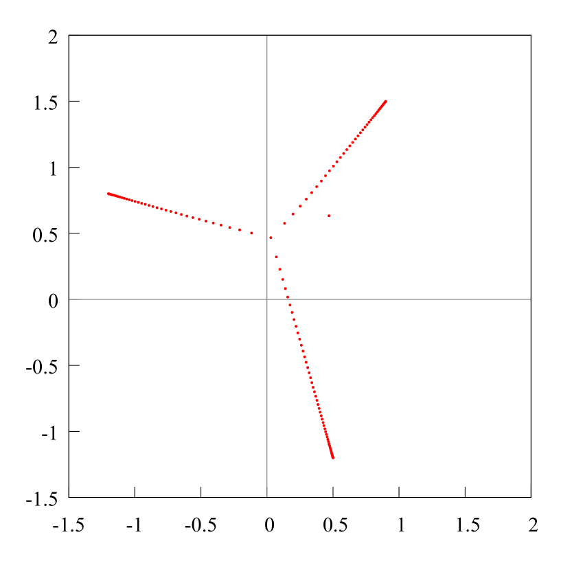
Figure 3. The poles of the Padé approximant $[130/130]_{f}$ approximate a Chebotarev point $v_{130}$ for the $S$-compact $S_{130}$. When $n\to\infty$ we have that $v_{n}\to v$ is a classical Chebotarev point. There is one spurious pole of the Padé approximant $[130/130]_{f}$, it is accompanied by a spurious zero of the Padé approximant $[130/130]_{f}$ (see fig. 4).

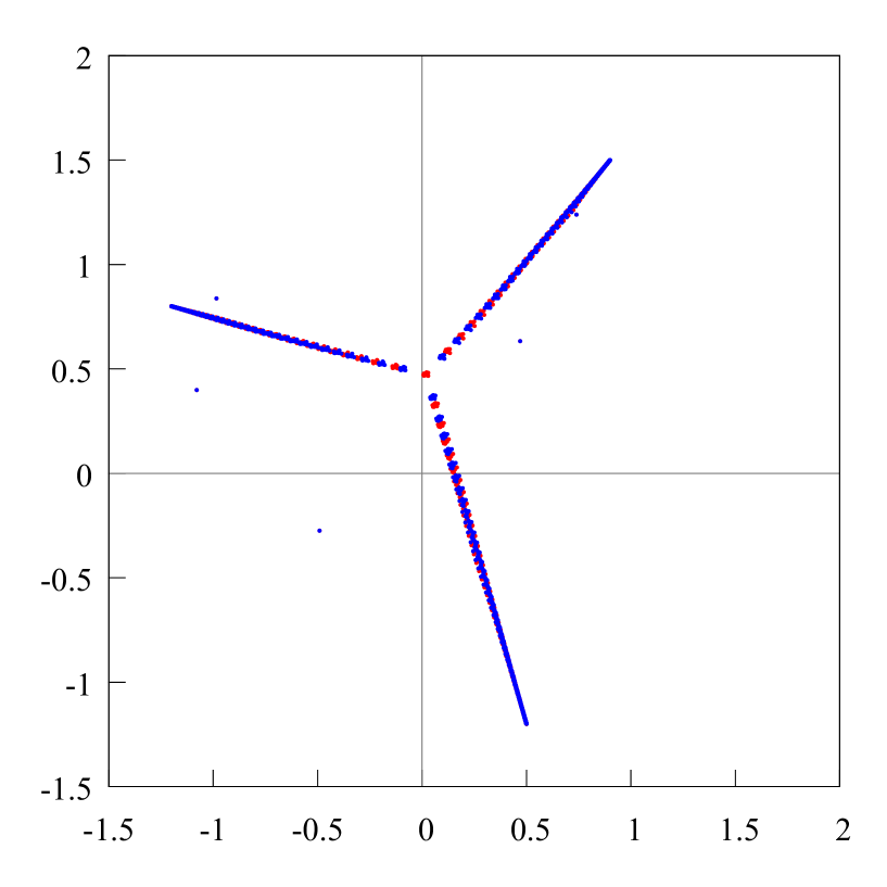
Figure 5. Zeros and poles of the diagonal Padé approximants $[n/n]_{f}$, $n=121,\dots,130$, of the function $f(z)=1/\{(z-(-1.2+i\cdot 0.8))(z-(0.9+i\cdot 1.5))(z-(0.5-i\cdot 1.2))\}^{1/3}$ for each $n=121,\dots,130$ are distributed in the complex plane accordingly to the electrostatical model by E. A. Rakhmanov [52]. Since the genus of the Riemann surface is $1$, there might be at most one Froissart doublet for each $n$. Here are observed 5 Froissart doublets. In full compliance with the Rakhmanov model [52] the $n$-th Froissart doublet “attracts” the Stahl $S$-compact $S_{n}$, $n\in\{121,\dots,130\}$, comp. fig. 1.

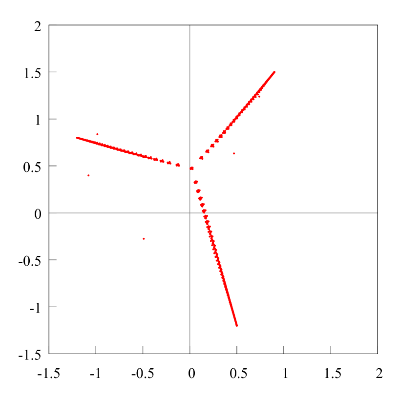
Figure 6. For the function $f(z)=1/\{(z-(-1.2+i\cdot 0.8))(z-(0.9+i\cdot 1.5))(z-(0.5-i\cdot 1.2))\}^{1/3}$ poles of the Padé approximants $[n/n]_{f}$, $n=121,\dots,130$, approximate a Chebotarev point. However, the presence of Froissart doublets changes slightly the position of the existing points $v_{n}$ depending on $n\in\{121,\dots,130\}$. This is in full accordance with the Rakhmanov model [52].

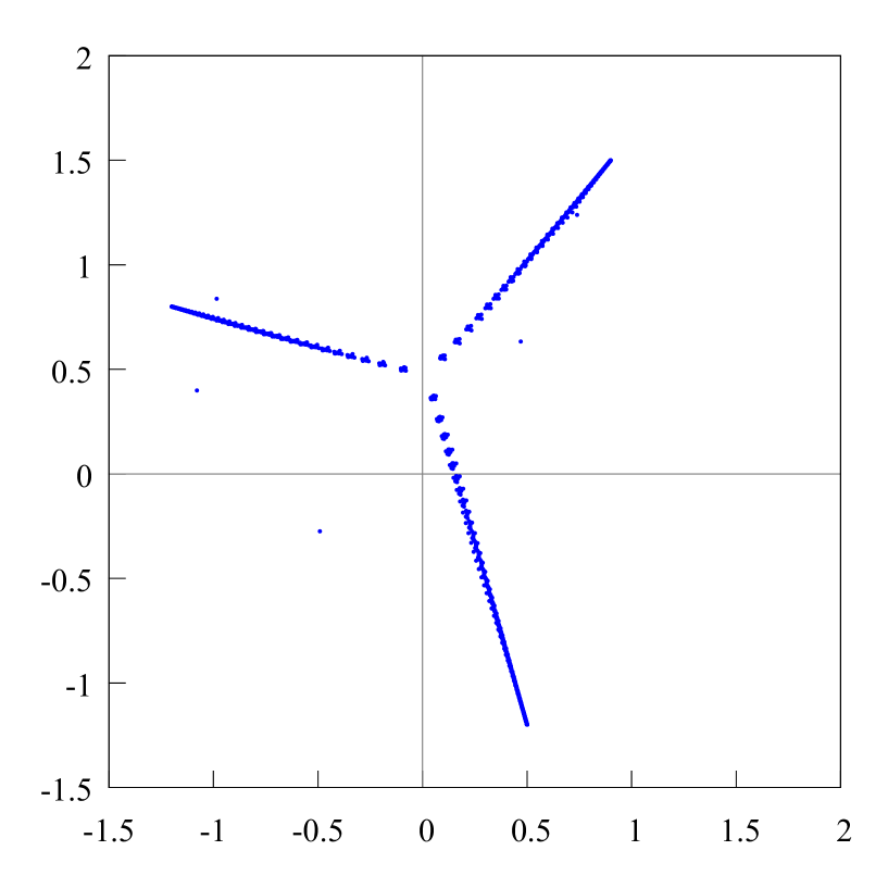
Figure 7. Zeros of the Padé approximants $[n/n]_{f}$, $n=121,\dots,130$, for the function $f(z)=1/\{(z-(-1.2+i\cdot 0.8))(z-(0.9+i\cdot 1.5))(z-(0.5-i\cdot 1.2))\}^{1/3}$. The Chebotarev point should not be approximated by zeros of the Padé approximant $[n/n]_{f}$.

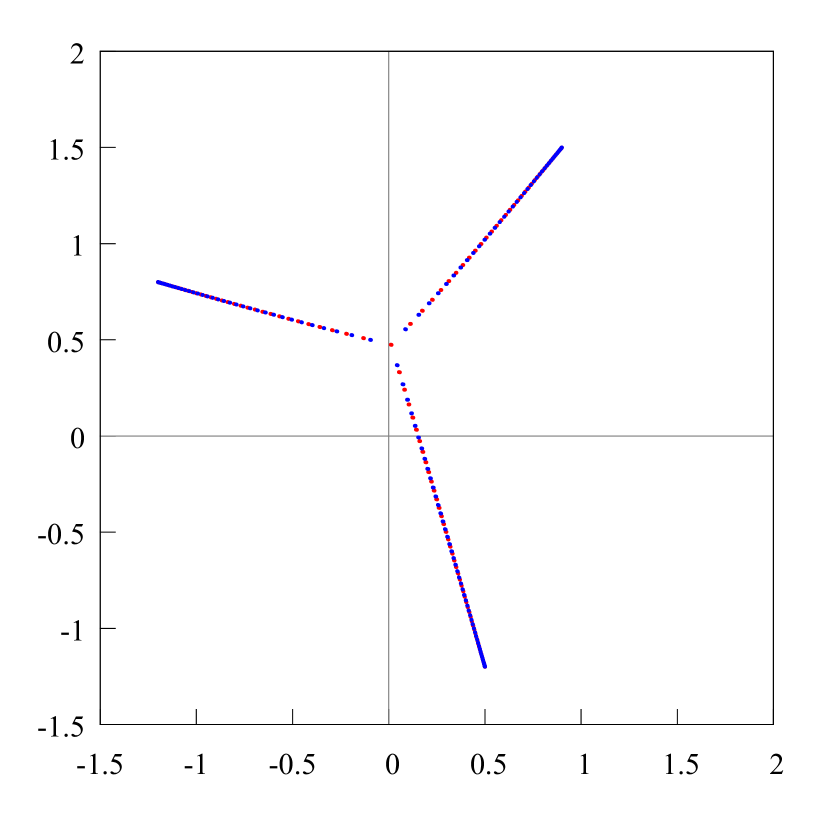
Figure 8. Zeros and poles of the diagonal Padé approximants $[n/n]_{f}$ when $n=131$ and $n=132$ of the function $f(z)=1/\{(z-(-1.2+i\cdot 0.8))(z-(0.9+i\cdot 1.5))(z-(0.5-i\cdot 1.2))\}^{1/3}$. The Froissart doublets are not present when $n=131$ and $n=132$. Therefore the $S$-compacts $S_{131}$ and $S_{132}$ are practically the same.

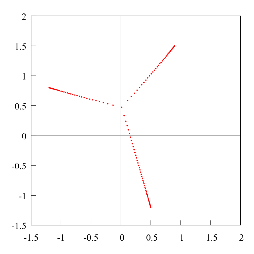
Figure 9. Poles of the diagonal Padé approximants $[n/n]_{f}$ when $n=131$ and $n=132$ of the function $f(z)=1/\{(z-(-1.2+i\cdot 0.8))(z-(0.9+i\cdot 1.5))(z-(0.5-i\cdot 1.2))\}^{1/3}$. The Froissart doublets are not present when $n=131$ and $n=132$. Therefore, the Chebotarev points $v_{131}$ and $v_{132}$, approximated by the poles of the diagonal Padé approximants $[n/n]_{f}$ when $n=131$ and $n=132$, are very close to each other and are practically the same.

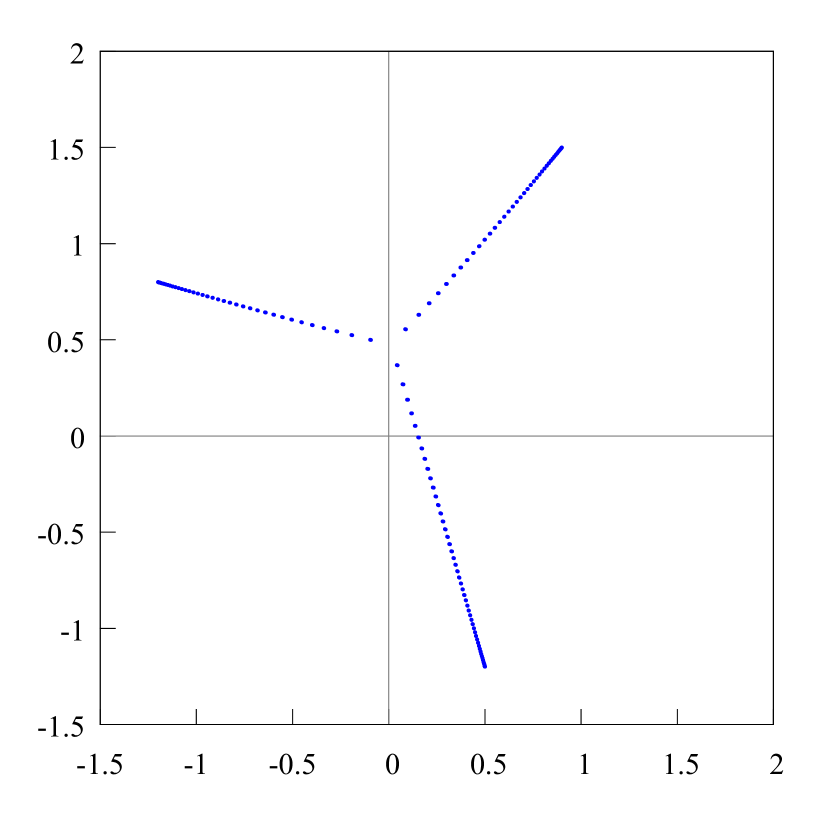
Figure 10. Zeros of the Padé approximants $[n/n]_{f}$ when $n=131$ and $n=132$ of the function $f(z)=1/\{(z-(-1.2+i\cdot 0.8))(z-(0.9+i\cdot 1.5))(z-(0.5-i\cdot 1.2))\}^{1/3}$ do not approximate the Chebotarev points $v_{131}$ and $v_{132}$. The Froissart doublets are not present when $n=131$ and $n=132$. Therefore the zeros the diagonal Padé approximants $[n/n]_{f}$ when $n=131$ and $n=132$ are practically the same.

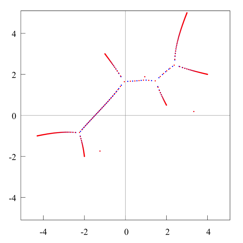
Figure 11. Zeros and poles of the diagonal Padé approximants $[103/103]_{f}$ of the function $f(z)=1/\bigl{\{}(z+(4.3+i\cdot 1.))(z-(2.+i\cdot.5))\*(z+(2.+i\cdot 2.))\*(z+(1.-i\cdot 3.))(z-(4.+i\cdot 2.))(z-(3.+i\cdot 5.))\bigr{\}}^{1/6}$. In the limit when $n\to\infty$ the zeros and poles of the diagonal Padé approximants $[n/n]_{f}$ are distributed accordingly with Stahl’s theorem [62]. Under fixed $n=103$ these zeros and poles are distributed in a plane, accordingly to the electrostatical model by Rakhmanov [52]. Since the genus of the Riemann surface is $1$, for each $n$ there might be no more than 4 Froissart doublets. Here are observed 3 Froissart doublets. When $n=103$, in full compliance with the Rakhmanov model, the Froissart doublets “attract” the Stahl $S$-compact $S_{103}$.

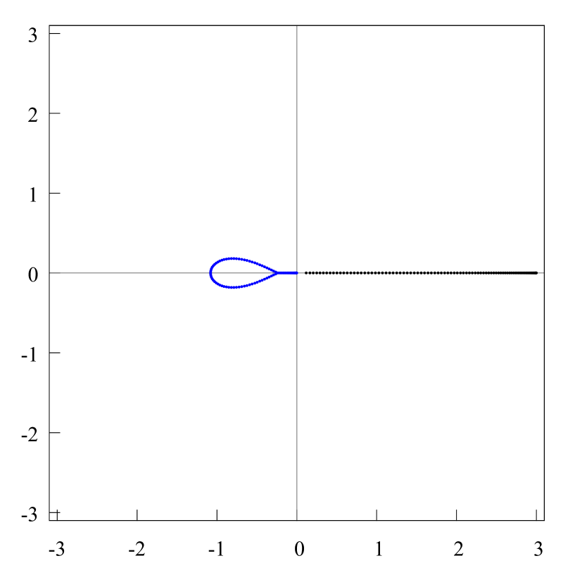
Figure 13. The distribution of the zeros of the Hermite-Padé polynomial $Q_{90,0}$ (blue points) and $Q_{90,2}$ (black points) for the set of three functions $[1,f_{1},f_{2}]$, where $f_{1}(z)=\sqrt{(z+1)/z}$, $f_{2}=\sqrt{(z-3)/z}$. The zeros of the polynomial $Q_{90,0}$ (blue points, comp fig. 33) create a third extremal compact $F_{0}$, which “separates” the compacts $F_{1}$ and $F_{2}$.

Figure 14. The distribution of the zeros of the Hermite-Padé polynomials $Q_{120,0}$ (blue points), $Q_{120,1}$ (red points) and $Q_{120,2}$ (black points) for a set of three functions $[1,f_{1},f_{2}]$, where $f_{1}(z)=\sqrt{(z-1)/(z+1)}$, $f_{2}(z)=\sqrt{(z-2)/(z+2)}$. The sets of branch points of the functions $f_{1}$ and $f_{2}$ do not intersect each other, and thus the pair $f_{1},f_{2}$ create an Angelesco system. However, the distribution of the zeros of the Hermite-Padé polynomials for this system is the same as the distribution for the Nikishin system $f_{1}(z)=\left((z-1)/(z+1)\right)^{1/3}\left((z-2)/(z+2)\right)^{1/3}$, $f_{2}(z)=\left((z-1)/(z+1)\right)^{2/3}\left((z-2)/(z+2)\right)^{1/3}$; see fig. 15–17.

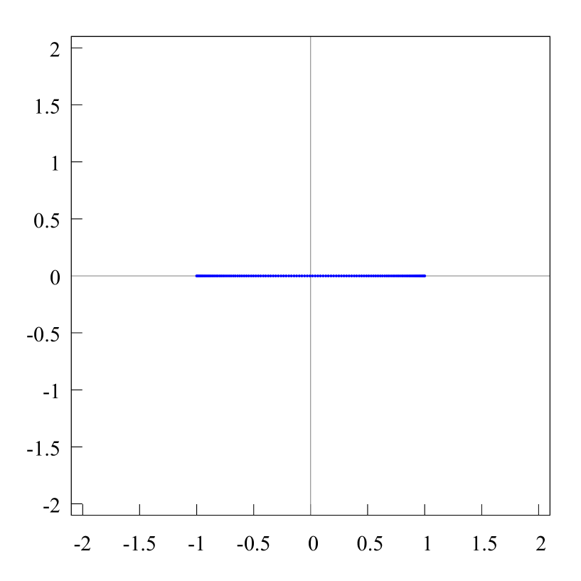
Figure 19. The distribution of the zeros of the Hermite-Padé polynomials $Q_{120,0}$ (blue points) for a set of three functions $[1,f_{1},f_{2}]$, where $f_{1}(z)=\sqrt[3]{(z-1)/(z+1)}$, $f_{2}(z)=\sqrt[3]{(z-2)/(z+2)}$. The pair $f_{1},f_{2}$ create an Angelesco system. However, the distribution of the zeros of the Hermite-Padé polynomials for this system is the same as the distribution for the Nikishin system $f_{1}(z)=\left((z-1)/(z+1)\right)^{1/3}\left((z-2)/(z+2)\right)^{1/3}$, $f_{2}(z)=\left((z-1)/(z+1)\right)^{2/3}\left((z-2)/(z+2)\right)^{1/3}$; comp. fig. 17.

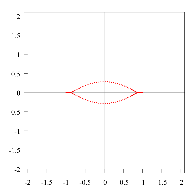
Figure 20. The distribution of the zeros of the Hermite-Padé polynomials $Q_{120,1}$ (red points) for a set of three functions $[1,f_{1},f_{2}]$, where $f_{1}(z)=\sqrt[3]{(z-1)/(z+1)}$, $f_{2}(z)=\sqrt[3]{(z-2)/(z+2)}$. The pair $f_{1},f_{2}$ create an Angelesco system. However, the distribution of the zeros of the Hermite-Padé polynomials for this system is the same as the distribution for the Nikishin system $f_{1}(z)=\left((z-1)/(z+1)\right)^{1/3}\left((z-2)/(z+2)\right)^{1/3}$, $f_{2}(z)=\left((z-1)/(z+1)\right)^{2/3}\left((z-2)/(z+2)\right)^{1/3}$; comp. fig. 17.

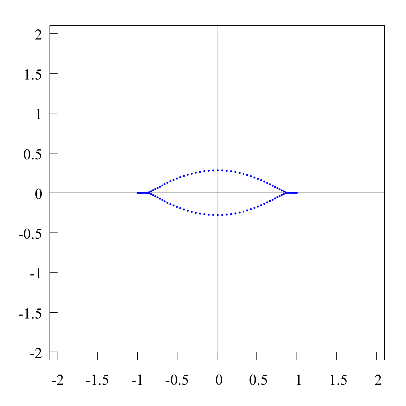
Figure 22. The distribution of the zeros of the Hermite-Padé polynomials $Q_{120,0}$ (blue points) for a set of three functions $[1,f_{1},f_{2}]$, where $f_{1}(z)=\sqrt{(z-1)/(z+1)}$, $f_{2}(z)=\sqrt[3]{(z-2)/(z+2)}$. The pair $f_{1},f_{2}$ create an Angelesco system. However, the distribution of the zeros of the Hermite-Padé polynomials for this system is different than the distribution of the pair $f_{1}(z)=\sqrt[3]{(z-1)/(z+1)}$, $f_{2}(z)=\sqrt[3]{(z-2)/(z+2)}$. comp. fig. 18–20. This confirms that the distribution of the zeros of the Hermite-Padé polynomials depends not only on the geometrical position of the branch points, but also of the type of the branch points.

Figure 23. The distribution of the zeros of the Hermite-Padé polynomials $Q_{120,1}$ (red points) for a set of three functions $[1,f_{1},f_{2}]$, where $f_{1}(z)=\sqrt{(z-1)/(z+1)}$, $f_{2}(z)=\sqrt[3]{(z-2)/(z+2)}$. The pair $f_{1},f_{2}$ create an Angelesco system. However, the distribution of the zeros of the Hermite-Padé polynomials for this system is different than the distribution of the pair $f_{1}(z)=\sqrt[3]{(z-1)/(z+1)}$, $f_{2}(z)=\sqrt[3]{(z-2)/(z+2)}$. comp. fig. 18–20. This confirms that the distribution of the zeros of the Hermite-Padé polynomials depends not only on the geometrical position of the branch points, but also of the type of the branch points.

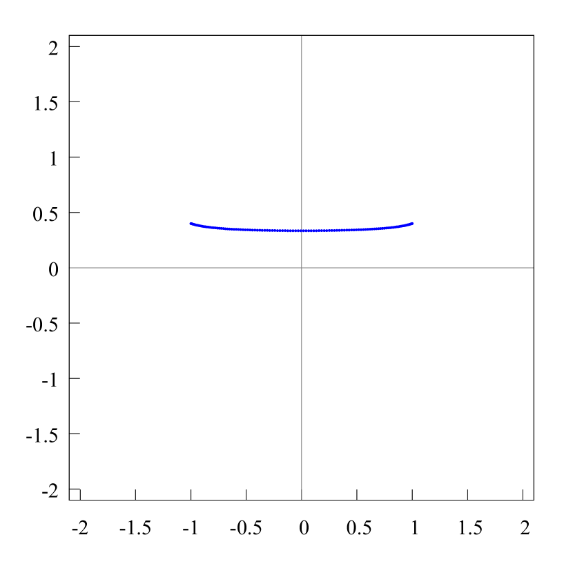
Figure 25. The distribution of the zeros of the Hermite-Padé polynomials $Q_{120,0}$ (blue points) for a set of three functions $[1,f_{1},f_{2}]$, where $f_{1}(z)=\sqrt[3]{(z-(1+i\cdot 0.4))/(z-(-1+i\cdot 0.4))}$, $f_{2}(z)=\sqrt[3]{(z-2)/(z+2)}$. The set of the branch points of the functions $f_{1}$ and $f_{2}$ do not intersect each other, thus the pair $f_{1},f_{2}$ create an Angelesco system; comp. 18–20.

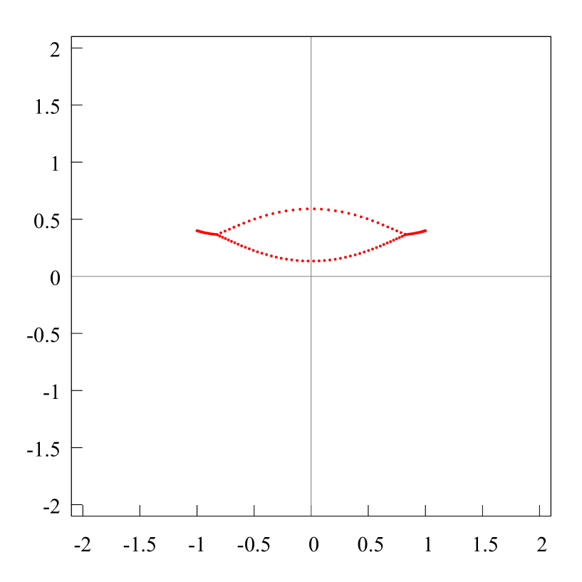
Figure 26. The distribution of the zeros of the Hermite-Padé polynomials $Q_{120,1}$ (red points) for a set of three functions $[1,f_{1},f_{2}]$, where $f_{1}(z)=\sqrt[3]{(z-(1+i\cdot 0.4))/(z-(-1+i\cdot 0.4))}$, $f_{2}(z)=\sqrt[3]{(z-2)/(z+2)}$. The set of the branch points of the functions $f_{1}$ and $f_{2}$ do not intersect each other, thus the pair $f_{1},f_{2}$ create an Angelesco system; comp. 18–20.

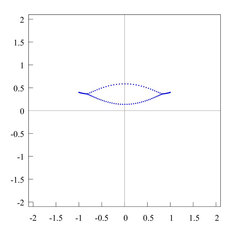
Figure 28. The distribution of the zeros of the Hermite-Padé polynomials $Q_{120,0}$ (blue points) for a set of three functions $[1,f_{1},f_{2}]$, where $f_{1}(z)=\sqrt{(z-(1+i\cdot 0.4))/(z-(-1+i\cdot 0.4))}$, $f_{2}(z)=\sqrt[3]{(z-2)/(z+2)}$. The set of the branch points of the functions $f_{1}$ and $f_{2}$ do not intersect each other, thus the pair $f_{1},f_{2}$ create an Angelesco system; comp. 21–23.

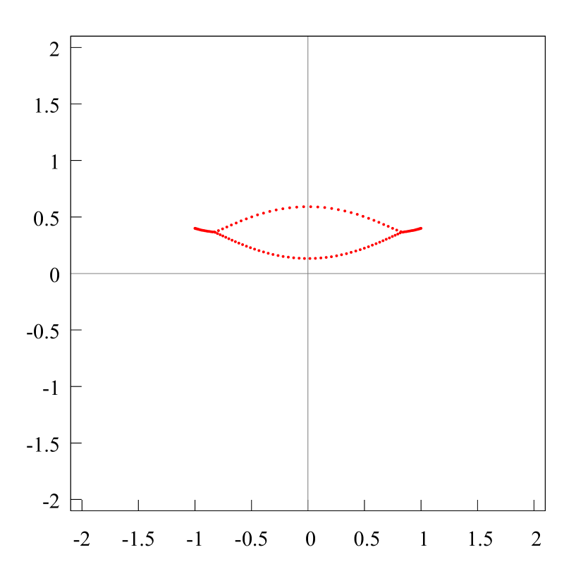
Figure 29. The distribution of the zeros of the Hermite-Padé polynomials $Q_{120,1}$ (red points) for a set of three functions $[1,f_{1},f_{2}]$, where $f_{1}(z)=\sqrt{(z-(1+i\cdot 0.4))/(z-(-1+i\cdot 0.4))}$, $f_{2}(z)=\sqrt[3]{(z-2)/(z+2)}$. The set of the branch points of the functions $f_{1}$ and $f_{2}$ do not intersect each other, thus the pair $f_{1},f_{2}$ create an Angelesco system; comp. 21–23.

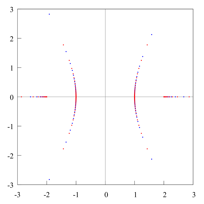
Figure 31. The distribution of the zeros of the Hermite-Padé polynomials $Q_{120,0}$ (blue points) and $Q_{120,1}$ (red points) for a set of three functions $[1,f_{1},f_{2}]$, where $f_{1}(z)=\left((z-1)/(z+1)\right)^{1/3}\left((z-2)/(z+2)\right)^{1/3}$, $f_{2}(z)=\left((z-1)/(z+1)\right)^{2/3}\left((z-2)/(z+2)\right)^{-1/3}$. The pair $f_{1},f_{2}$ create a Nikishin system.

Figure 35. The distribution of the Hermite-Padé polynomials $Q_{180,0}$ (blue points), $Q_{180,1}$ (red points), $Q_{180,2}$ (black points) for two functions $f_{1}(z)=\sqrt{(1.0-(-1.0+i\cdot 0.6)\zeta)(1.0-(1.0+i\cdot 0.6)\zeta)}$, $f_{2}(z)=\sqrt{(1.0-(-.65-i\cdot 0.6)\zeta)(1.0-(.65-i\cdot 0.6)\zeta)}$. The branch points have come closer to each other, however they are still far enough from each other and there is no collision of the supports of the equilibrium measures. It is clearly seen, that the upper extremal compact $F_{1}$ has strongly bent towards the lower extremal compact $F_{2}$. The third extremal compact $F_{0}$, as before, separates $F_{1}$ and $F_{2}$.

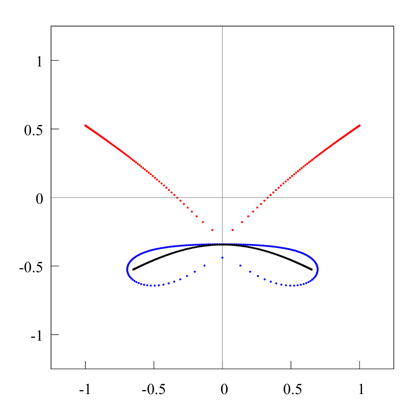
Figure 37. The distribution of the Hermite-Padé polynomials $Q_{180,0}$ (blue points), $Q_{180,1}$ (red points), $Q_{180,2}$ (black points) for two functions $f_{1}(z)=1/\sqrt{(z-(-1.0+i\cdot 0.525))(z-(1.0+i\cdot 0.525))}$, $f_{2}(z)=1/\sqrt{(z-(-.65-i\cdot 0.525))(z-(.65-i\cdot 0.525))}$. It is clearly seen, that the upper extremal compact $F_{1}$ has even strongly bent towards the lower extremal compact $F_{2}$. The third extremal compact $F_{0}$, as before, separates $F_{1}$ and $F_{2}$. The support of the equilibrium measure of the upper extremal compact $F_{1}$ starts to break down, while the second compact $F_{2}$ has hardly changed. The third extremal compact $F_{0}$, as before, separates the other two compacts from each other, but now it touches the second compact $F_{2}$.

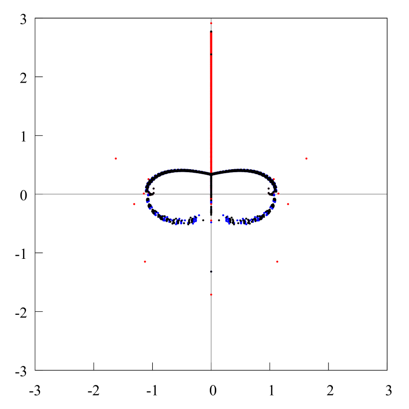
Figure 48. The distribution of the zeros of the Hermite-Padé polynomials $Q_{n,0}$ (blue points), $Q_{n,1}$ (red points), $Q_{n,2}$ (black points), $n=61,\dots,80$, for a set of three functions $[1,f,f^{2}]$, where $f(z)=(1-z^{2})^{1/4}(1-i\sqrt{3}\cdot 1.6z)^{-1/2}$. The Riemann sphere is decomposed into 3 domains by the zeros of the Hermite-Padé polynomials, one of them contains the infinity point, while the other two are symmetrical with respect to the imaginary axis. There is a pair of Froissart triplets inside these two domans for some $n\in\{61,\dots,80\}$, there is a pair of Froissart singlets in the complementary domains for some $n\in\{61,\dots,80\}$, there is one Froissart doublet on the negative part of the imaginary axis. This follows from the analysis of the next figures 49, 50, and 51.

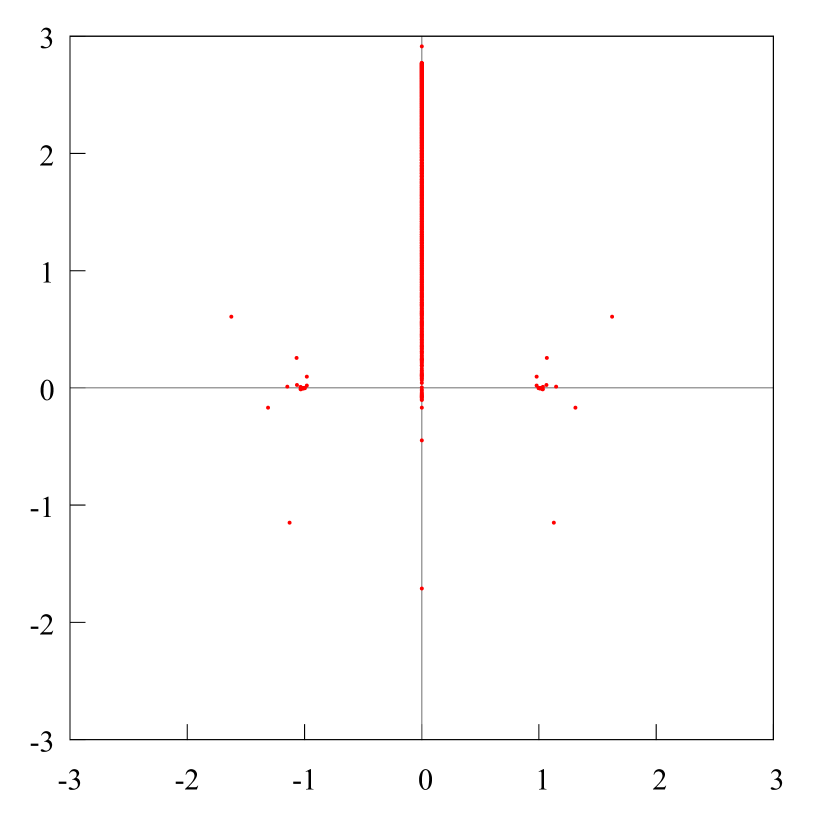
Figure 49. The distribution of the zeros of the Hermite-Padé polynomials $Q_{n,1}$ (red points), $n=61,\dots,80$, for a set of three functions $[1,f,f^{2}]$, where $f(z)=(1-z^{2})^{1/4}(1-i\sqrt{3}\cdot 1.6z)^{-1/2}$.

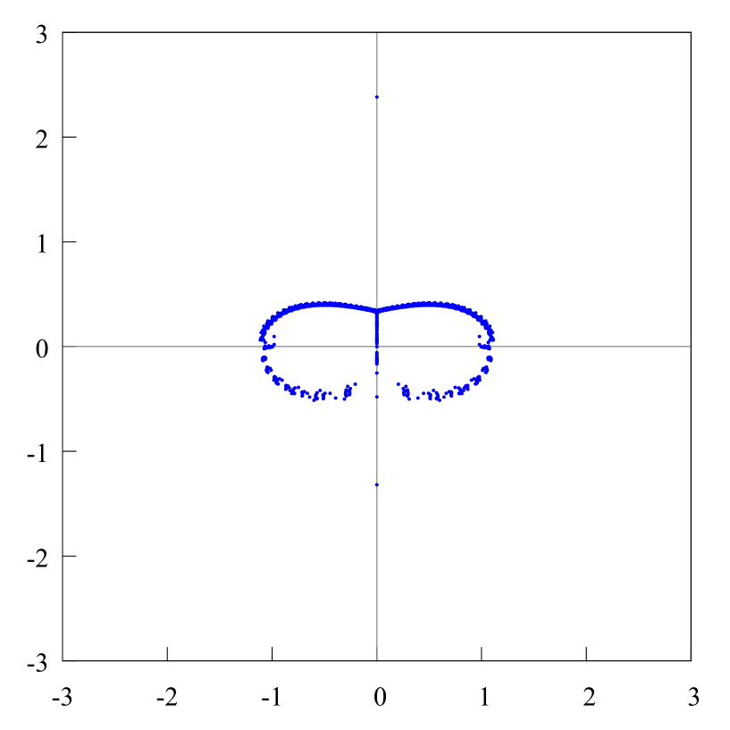
Figure 50. The distribution of the zeros of the Hermite-Padé polynomials $Q_{n,0}$ (blue points), $n=61,\dots,80$, for a set of three functions $[1,f,f^{2}]$, where $f(z)=(1-z^{2})^{1/4}(1-i\sqrt{3}\cdot 1.6z)^{-1/2}$.

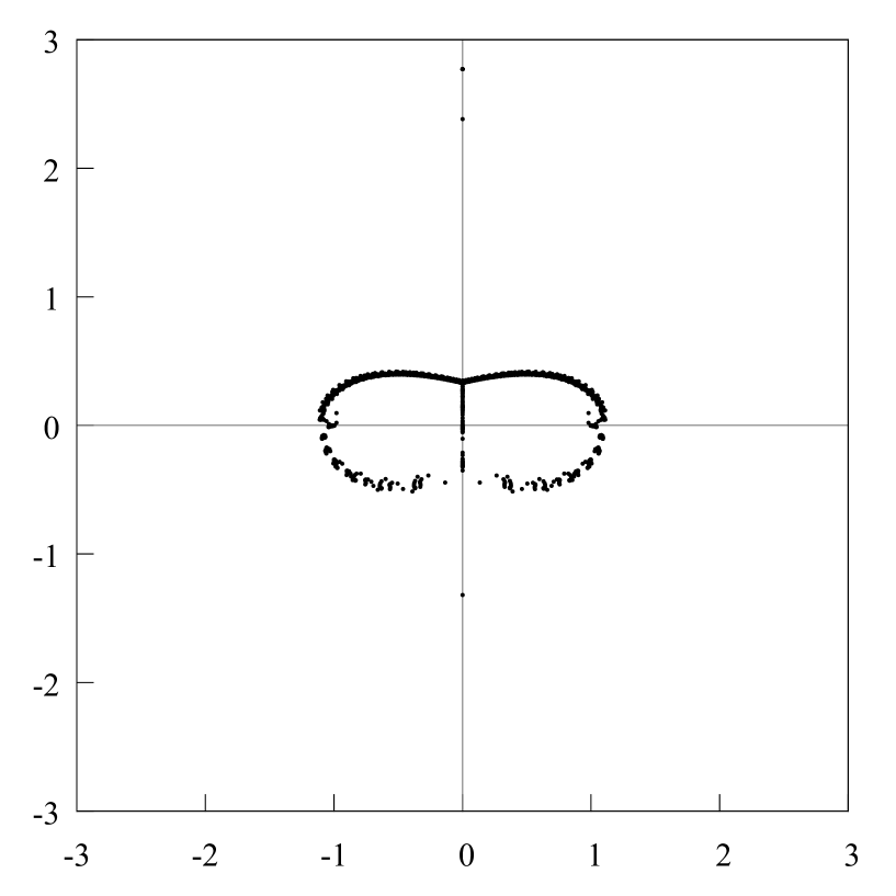
Figure 51. The distribution of the zeros of the Hermite-Padé polynomials $Q_{n,2}$ (black points), $n=61,\dots,80$, for a set of three functions $[1,f,f^{2}]$, where $f(z)=(1-z^{2})^{1/4}(1-i\sqrt{3}\cdot 1.6z)^{-1/2}$. There is a simple zero of the polynomial $Q_{n,2}$, $n=61,\dots,80$, on the positive part of the imaginary axis at the point $z\approx a$, $a=i\sqrt{3}\cdot 1.6$, corresponding to a simple pole of the function $f^{2}$ at the point $z=ia$.

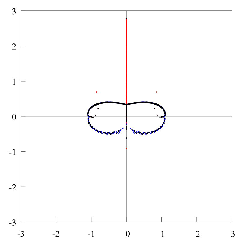
Figure 52. The distribution of the zeros of the Hermite-Padé polynomials $Q_{n,0}$ (blue points), $Q_{n,1}$ (red points), $Q_{n,2}$ (black points), $n=121,\dots,130$, for a set of three functions $[1,f,f^{2}]$, where $f(z)=(1-z^{2})^{1/4}(1-i\sqrt{3}\cdot 1.6z)^{-1/2}$. The Riemann sphere is decomposed into 3 domains by the zeros of the Hermite-Padé polynomials, one of them contains the infinity point, while the other two are symmetrical with respect to the imaginary axis. There is a pair of Froissart triplets inside these two domans for some $n\in\{121,\dots,130\}$, there is a pair of Froissart singlets in the complementary domains for some $n\in\{121,\dots,130\}$, there is a Froissart doublet on the negative part of the imaginary axis. This follows from the analysis of the next figures 53, 54 and 55.

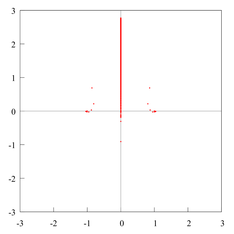
Figure 53. The distribution of the zeros of the Hermite-Padé polynomials $Q_{n,1}$ (red points), $n=121,\dots,130$, for a set of three functions $[1,f,f^{2}]$, where $f(z)=(1-z^{2})^{1/4}(1-i\sqrt{3}\cdot 1.6z)^{-1/2}$.

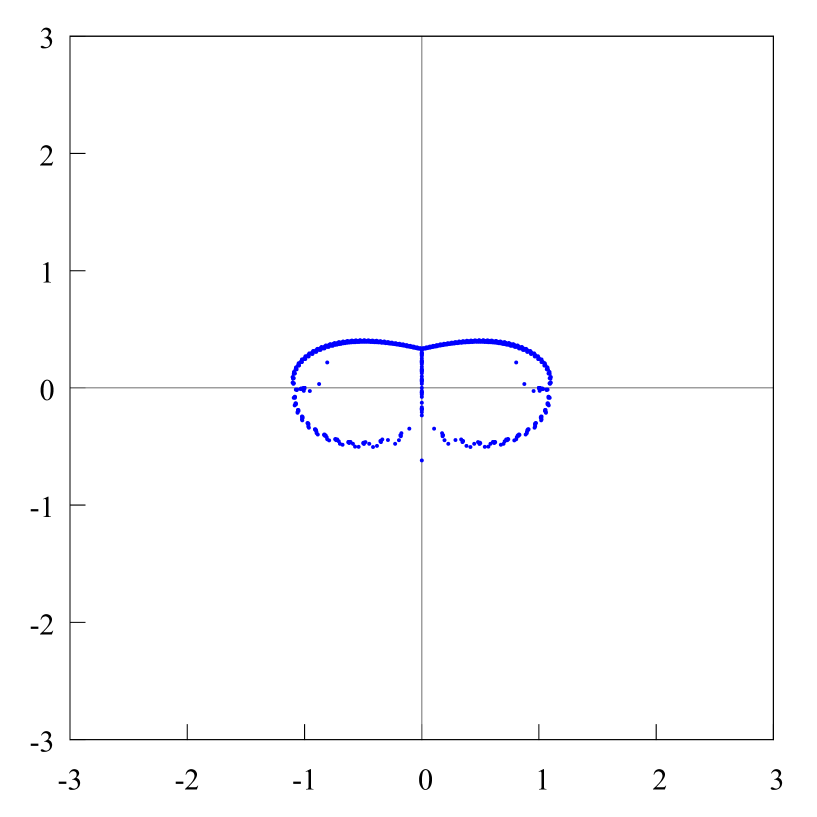
Figure 54. The distribution of the zeros of the Hermite-Padé polynomials $Q_{n,0}$ (blue points), $n=121,\dots,130$, for a set of three functions $[1,f,f^{2}]$, where $f(z)=(1-z^{2})^{1/4}(1-i\sqrt{3}\cdot 1.6z)^{-1/2}$.

Figure 55. The distribution of the zeros of the Hermite-Padé polynomials $Q_{n,2}$ (black points), $n=121,\dots,130$, for a set of three functions $[1,f,f^{2}]$, where $f(z)=(1-z^{2})^{1/4}(1-i\sqrt{3}\cdot 1.6z)^{-1/2}$. There is a simple zero of the polynomial $Q_{n,2}$, $n=121,\dots,130$, on the positive part of the imaginary axis at the point $z\approx a$, $a=i\sqrt{3}\cdot 1.6$, corresponding to a simple pole of the function $f^{2}$ at the point $z=ia$.

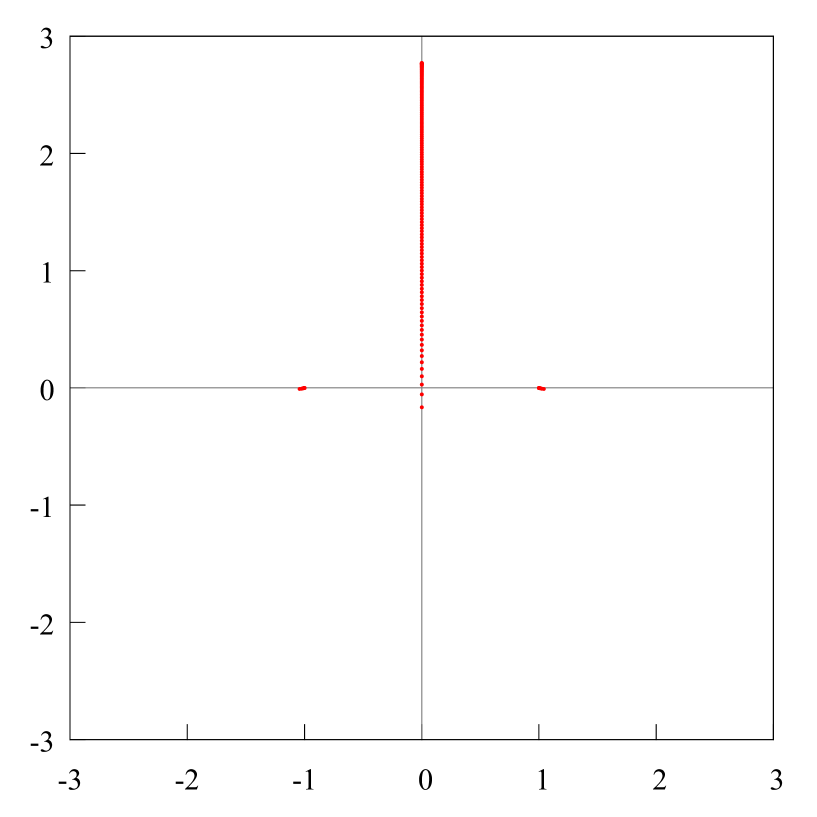
Figure 57. The distribution of the zeros of the Hermite-Padé polynomials $Q_{n,1}$ (red points), $n=121,\dots,130$, in the plane $\mathbb{C}_{z}$ for a set of three functions $[1,f,f^{2}]$, where $f(z)=(1-z^{2})^{1/4}(1-i\sqrt{3}\cdot 1.6z)^{-1/2}$. There are no Froissart zeros when $n=165$.

Figure 59. The distribution of the zeros of the Hermite-Padé polynomials $Q_{n,2}$ (black points), $n=121,\dots,130$, in the plane $\mathbb{C}_{z}$ for a set of three functions $[1,f,f^{2}]$, where $f(z)=(1-z^{2})^{1/4}(1-i\sqrt{3}\cdot 1.6z)^{-1/2}$. There is a simple zero of the polynomial $Q_{n,2}$, $n=121,\dots,130$, on the positive part of the imaginary axis at the point $z\approx a$, $a=i\sqrt{3}\cdot 1.6$, corresponding to a simple pole of the function $f^{2}$ at the point $z=ia$. There are no Froissart zeros when $n=165$.

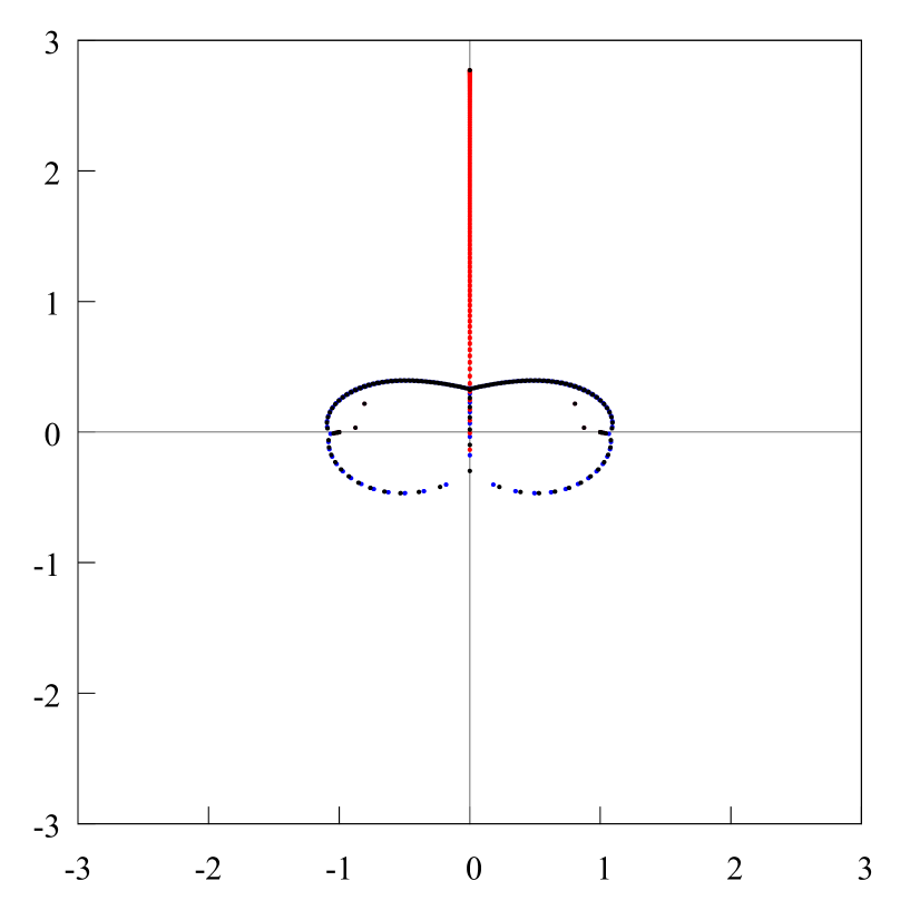
Figure 60. The distribution of the zeros of the Hermite-Padé polynomials $Q_{n,0}$ (blue points), $Q_{n,1}$ (red points), $Q_{n,2}$ (black points), $n=127,128$, for a set of three functions $[1,f,f^{2}]$, where $f(z)=(1-z^{2})^{1/4}(1-i\sqrt{3}\cdot 1.6z)^{-1/2}$. The Riemann sphere is decomposed into 3 domains by the zeros of the Hermite-Padé polynomials, one of them contains the infinity point, while the other two are symmetrical with respect to the imaginary axis. There is a pair of Froissart triplets inside these two domans for some $n\in\{127,128\}$, there is a pair of Froissart singlets in the complementary domains for some $n\in\{127,128\}$, there is one Froissart doublet on the negative part of the imaginary axis. This follows from the analysis of the next figures 61, 62 and 63.

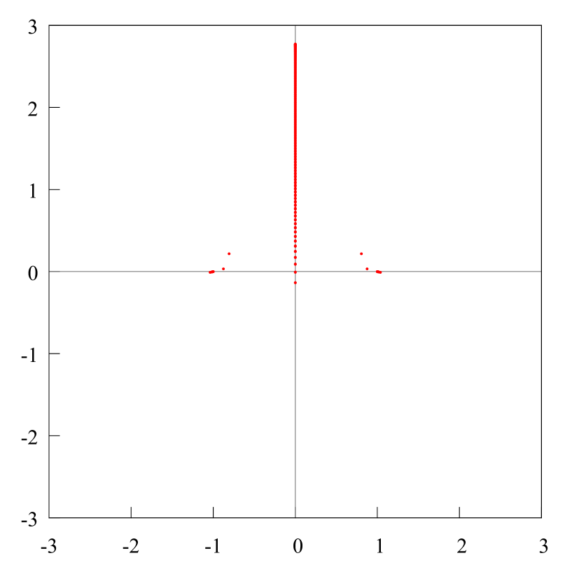
Figure 61. The distribution of the zeros of the Hermite-Padé polynomials $Q_{n,1}$ (red points), $n=127,128$, for a set of three functions $[1,f,f^{2}]$, where $f(z)=(1-z^{2})^{1/4}(1-i\sqrt{3}\cdot 1.6z)^{-1/2}$.

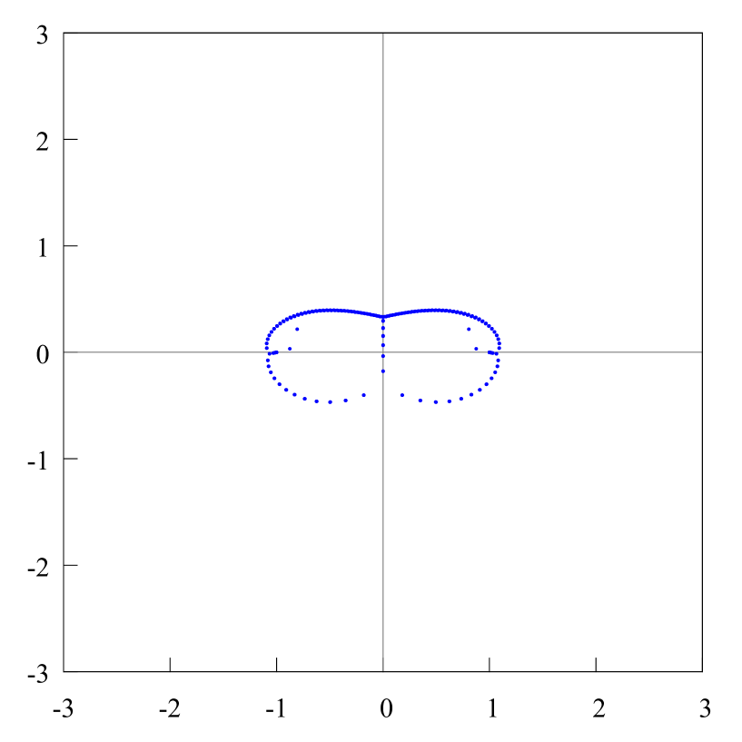
Figure 62. The distribution of the zeros of the Hermite-Padé polynomials $Q_{n,0}$ (blue points), $n=127,128$, for a set of three functions $[1,f,f^{2}]$, where $f(z)=(1-z^{2})^{1/4}(1-i\sqrt{3}\cdot 1.6z)^{-1/2}$.

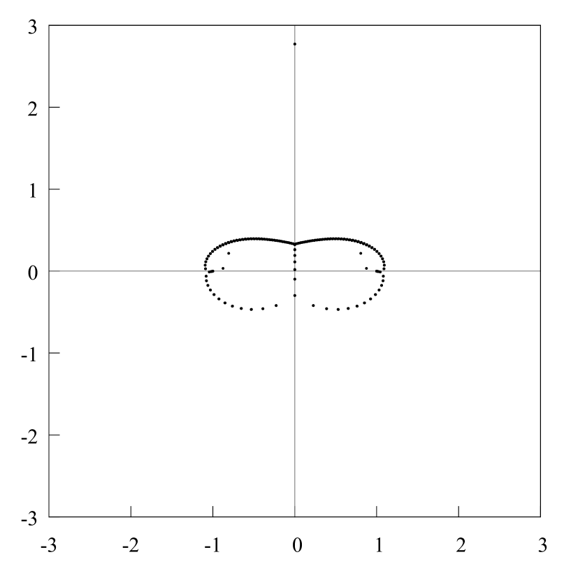
Figure 63. The distribution of the zeros of the Hermite-Padé polynomials $Q_{n,2}$ (black points), $n=127,128$, for a set of three functions $[1,f,f^{2}]$, where $f(z)=(1-z^{2})^{1/4}(1-i\sqrt{3}\cdot 1.6z)^{-1/2}$. There is a simple zero of the polynomial $Q_{n,2}$, $n=127,128$, on the positive part of the imaginary axis at the point $z\approx a$, $a=i\sqrt{3}\cdot 1.6$, corresponding to a simple pole of the function $f^{2}$ at the point $z=ia$.

Figure 66. The distribution of the zeros of the Hermite-Padé polynomials $Q_{n,0}$ (blue points), $n=121,\dots,130$, for a set of three functions $[1,f,f^{2}]$, where $f$ is a “perturbed” function: $f(z)=(1-z^{2})^{1/4}(1-(0.1+i\sqrt{3}\cdot 1.6)z)^{-1/2}$.

Figure 67. The distribution of the zeros of the Hermite-Padé polynomials $Q_{n,2}$ (black points), $n=121,\dots,130$, for a set of three functions $[1,f,f^{2}]$, where $f$ is a “perturbed” function: $f(z)=(1-z^{2})^{1/4}(1-(0.1+i\sqrt{3}\cdot 1.6)z)^{-1/2}$. There are a simple zeros of the polynomials $Q_{n,2}$, $n=121,\dots,130$, on the positive part of the imaginary axis at the point $z\approx a$, $a=0.1+i\sqrt{3}\cdot 1.6$, corresponding to a simple pole of the function $f^{2}$ at the point $z=ia$.

Figure 68. The distribution of the zeros of the Hermite-Padé polynomials $Q_{n,0}$ (blue points), $Q_{n,1}$ (red points), $Q_{n,2}$ (black points) when $n=166,\dots,170$ for a set of three functions $[1,f,f^{2}]$, where $f(z)=(1-z^{2})^{1/4}(1-i\sqrt{3}\cdot 0.9z)^{-1/2}$. The Riemann sphere is decomposed into 3 domains by the zeros of the Hermite-Padé polynomials, one of them contains the infinity point, while the other two are symmetrical with respect to the imaginary axis. There is a pair of Froissart triplets inside these two domans for two $n$ of $n\in\{166,\dots,170\}$. This follows from the analysis of the next figures 69, 70, 71. There are no Froissart points in the complementary domains for $n=166,\dots,170$.

Figure 69. The distribution of the zeros of the Hermite-Padé polynomials $Q_{n,1}$ (red points) $n=166,\dots,170$ for a set of three functions $[1,f,f^{2}]$, where $f(z)=(1-z^{2})^{1/4}(1-i\sqrt{3}\cdot 0.9z)^{-1/2}$.

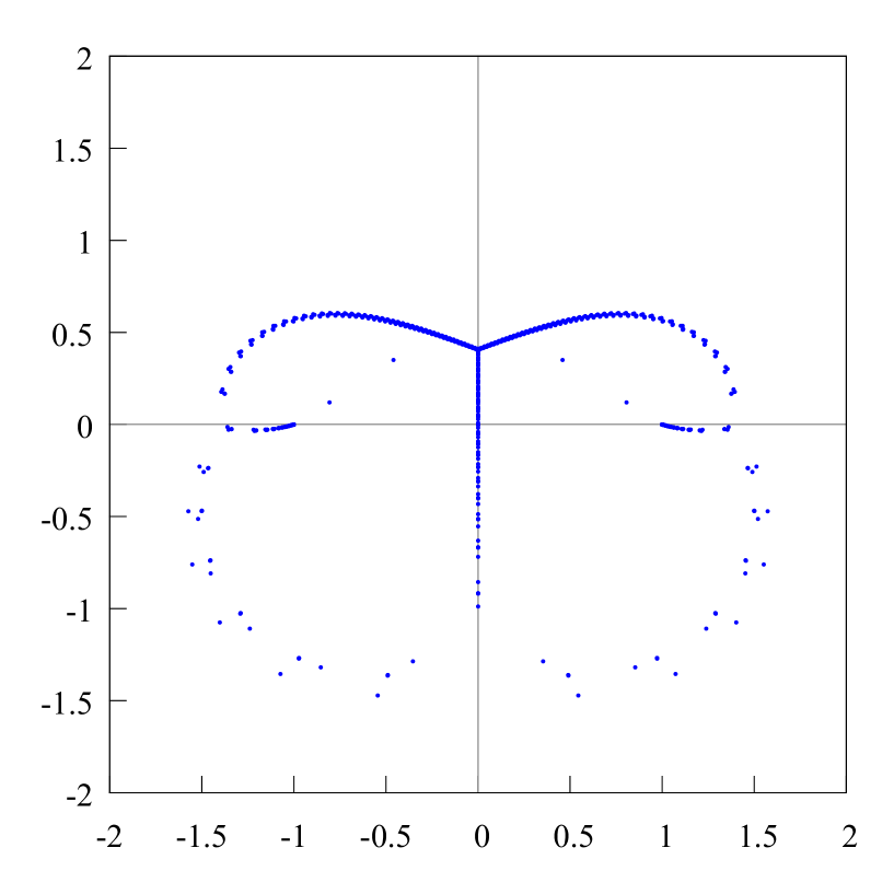
Figure 70. The distribution of the zeros of the Hermite-Padé polynomials $Q_{n,0}$ (blue points), $n=166,\dots,170$, for a set of three functions $[1,f,f^{2}]$, where $f(z)=(1-z^{2})^{1/4}(1-i\sqrt{3}\cdot 0.9z)^{-1/2}$.

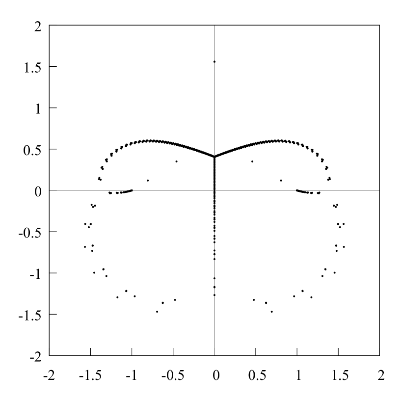
Figure 71. The distribution of the zeros of the Hermite-Padé polynomials $Q_{n,2}$ (black points), $n=166,\dots,170$, for a set of three functions $[1,f,f^{2}]$, where $f(z)=(1-z^{2})^{1/4}(1-i\sqrt{3}\cdot 0.9z)^{-1/2}$. There are simple zeros of the polynomials $Q_{n,2}$, $n=166,\dots,170$, on the positive part of the imaginary axis at the point $z\approx a$, $a=i\sqrt{3}\cdot 0.9$, corresponding to a simple pole of the function $f^{2}$ at the point $z=ia$.

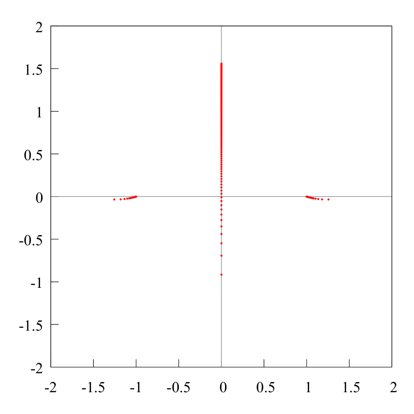
Figure 73. The distribution of the zeros of the Hermite-Padé polynomial $Q_{187,1}$ (red points), when $n=187$ for a set of three functions $[1,f,f^{2}]$, where $f(z)=(1-z^{2})^{1/4}(1-i\sqrt{3}\cdot 0.9z)^{-1/2}$.

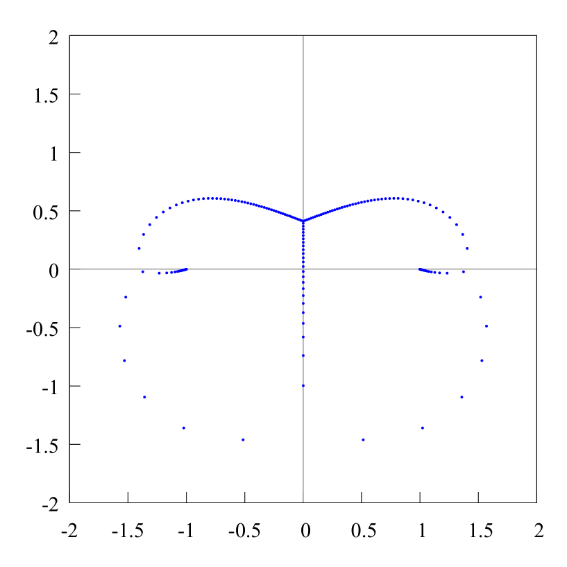
Figure 74. The distribution of the zeros of the Hermite-Padé polynomial $Q_{187,0}$ (blue points), when $n=187$ for a set of three functions $[1,f,f^{2}]$, where $f(z)=(1-z^{2})^{1/4}(1-i\sqrt{3}\cdot 0.9z)^{-1/2}$.

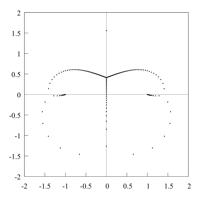
Figure 75. The distribution of the zeros of the Hermite-Padé polynomial $Q_{187,2}$ (black points), when $n=187$ for a set of three functions $[1,f,f^{2}]$, where $f(z)=(1-z^{2})^{1/4}(1-i\sqrt{3}\cdot 0.9z)^{-1/2}$. There is a simple zero of the polynomial $Q_{187,2}$ on the positive part of the imaginary axis at the point $z\approx a$, $a=i\sqrt{3}\cdot 0.9$, corresponding to a simple pole of the function $f^{2}$ at the point $z=ia$.

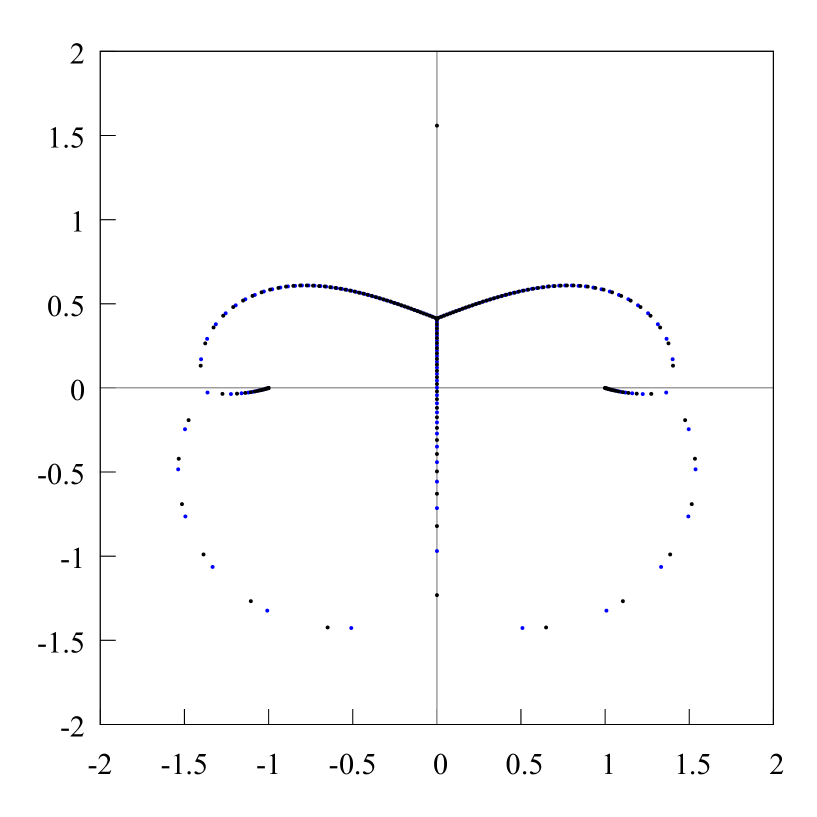
Figure 76. The distribution of the zeros of the Hermite-Padé polynomials $Q_{180,0},Q_{180,2}$ (blue and black points), when $n=180$ for a set of three functions $[1,f,f^{2}]$, where $f(z)=(1-z^{2})^{1/4}(1-i\sqrt{3}\cdot 0.9z)^{-1/2}$. There is a simple zero of the polynomial $Q_{180,2}$ on the positive part of the imaginary axis at the point $z\approx a$, $a=i\sqrt{3}\cdot 0.9$, corresponding to a simple pole of the function $f^{2}$ at the point $z=ia$.

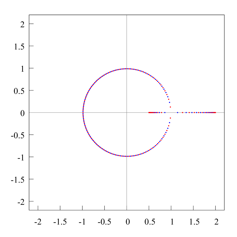
Figure 78. The distribution of zeros and poles of the two-point Padé approximant (at points $z=0$ and $z=\infty$) of the function $f(z)=\sqrt{(z-a)/(z-b)}$, $a=.5$, $b=2$. Here are selected two “different” branches of the function $f$: $f_{0}(z)=\sqrt{(z-.5)/(z-2)}$, $f_{\infty}(z)=-\sqrt{(z-.5)/(z-2)}$. There is one Chebotarev point $v=\sqrt{ab}=1$ of zero density on the Buslaev compact. From this can be seen, that this point cannot be calculated using of the two-point Padé approximants, comp. 4; contrary to the case with classical Padé approximants (see fig. 3, 2)

References

- [1] A. I. Aptekarev, V. A. Kalyagin, “Asymptotic behavior of an -th degree root of polynomials of simultaneous orthogonality, and algebraic functions”, Russian. Akad. Nauk SSSR Inst. Prikl. Mat. Preprint, 1986, No 60, 18 pp.
- [2] A. I. Aptekarev, “Asymptotics of Hermite–Pade approximants for a pair of functions with branch points (Russian)”, Dokl. Akad. Nauk, 422:4 (2008), 443–445; translation in Dokl. Math., 78:2 (2008), 717–719.
- [3] A. I. Aptekarev, “Integrable Semidiscretization of Hyperbolic Equations – “Computational” Dispersion and Multidimensional Perspective”, Keldysh Institute preprints, 2012, 020, 28.
- [4] A. I. Aptekarev, A. B. J. Kuijlaars, W. Van Assche, “Asymptotics of Hermite–Pade rational approximants for two analytic functions with separated pairs of branch points (case of genus )”, Art. ID rpm007, Int. Math. Res. Pap. IMRP, 2008, 128 pp.
- [5] A. I. Aptekarev, V. G. Lysov, “Systems of Markov functions generated by graphs and the asymptotics of their Hermite–Padé approximants”, Mat. Sb., 201:2 (2010), 29–78.
- [6] A. I. Aptekarev, V. G. Lysov, D. N. Tulyakov, “Random matrices with external source and the asymptotic behaviour of multiple orthogonal polynomials”, Mat. Sb., 202:2 (2011), 3–56.
- [7] Alexander I. Aptekarev, Maxim L. Yattselev, Padé approximants for functions with branch points – strong asymptotics of Nuttall–Stahl polynomials, http://arxiv.org/abs/1109.0332, 2011, 45 pp.
- [8] A. I. Aptekarev, A. Kuijlaars, “Hermite–Padé approximations and multiple orthogonal polynomial ensembles”, Uspekhi Mat. Nauk, 66:6(402) (2011), 123–190.
- [9] A. I. Aptekarev, V. I. Buslaev, A. Martínez-Finkelshtein, S. P. Suetin, “Padé approximants, continued fractions, and orthogonal polynomials”, Uspekhi Mat. Nauk, 66:6(402) (2011), 37–122.
- [10] Aptekarev A.I., Tulyakov D.N., “Geometry of Hermite–Pade approximants for system of functions with three branch points”, Keldysh Institute preprints, 2012, No 77, 25 p. library.keldysh.
- [11] A. I. Aptekarev, D. N. Tulyakov, “Abelian integral of Nuttall on the Riemann surface of the cubic root of the third degree polynomial”, Keldysh Institute preprints, 2014, 015, 25.
- [12] W. Van Assche, J. Geronimo, A. R. J. Kuijlaars, “Riemann–Hilbert problems for multiple orthogonal polynomials”, Special functions 2000: current perspective and future directions, (Tempe, AZ, 23-59), NATO Sci. Ser. II Math. Phys. Chem., 30, Kluwer Acad. Publ., Dordrecht, 2001.
- [13] Van Assche, Walter, “Pade and Hermite–Padé approximation and orthogonality”, Surv. Approx. Theory, 2 (2006), 61–91.
- [14] Filipuk, Galina; Van Assche, Walter; Zhang, Lun, “Ladder operators and differential equations for multiple orthogonal polynomials”, 205204, J. Phys. A, 46:20 (2013), 24 pp.
- [15] Van Assche, Walter, “Nearest neighbor recurrence relations for multiple orthogonal polynomials”, J. Approx. Theory, 163:10 (2011), 1427–1448.
- [16] Baker, George A., Jr.; Graves-Morris, Peter, Pade approximants. Part I, II. With a foreword by Peter A. Carruthers, Encyclopedia of Mathematics and its Applications, 13, 14, Addison-Wesley Publishing Co., Reading, Mass., 1981.
- [17] D. Belkic, “Exact Signal-Noise Separation by Froissart Doublets in Fast Pade Transform for Magnetic Resonance Spectroscopy”, Chapter 3, Advances in Quantum Chemistry, 56, eds. John R. Sabin, Erkki J. Brandas, 2009, 95–179, 333 pp.
- [18] O. L. Ibryaeva, V. M. Adukov, “An algorithm for computing a Pade approximant with minimal degree denominator”, J. Comput. Appl. Math., 237:1 (2013), 529–541.
- [19] Lloyd N. Trefethen, Approximation theory and approximation practice, Society for Industrial and Applied Mathematics (SIAM), Philadelphia, PA, 2013, viii+305 pp. ISBN: 978-1-611972-39-9.
- [20] V. I. Buslaev, “Convergence of multipoint Padé approximants of piecewise analytic functions”, Mat. Sb., 204:2 (2013), 39–72.
- [21] V. I. Buslaev, A. Martínez-Finkelshtein, S. P. Suetin, “Method of interior variations and existence of -compact sets”, Analytic and geometric issues of complex analysis, Collected papers, Tr. Mat. Inst. Steklova, 279, MAIK Nauka/Interperiodica, Moscow, 2012, 31–58.
- [22] G. V. Chudnovsky, “Pade approximation and the Riemann monodromy problem”, Bifurcation phenomena in mathematical physics and related topics, (Proc. NATO Advanced Study Inst., Cargese, 1979), Adv. Study Inst. Ser., Ser. C: Math. Phys. Sci., 54, Reidel, Dordrecht-Boston, Mass., 1980, 449–510, NATO.
- [23] M. Froissart, “Approximation de Pade: application a la physique des particules elementaires”, Recherche Cooperative sur Programme (RCP), 9, eds. Carmona, J., Froissart, M., Robinson, D.W., Ruelle, D., Centre National de la Recherche Scientifique (CNRS), Strasbourg, 1969, 1–13.
- [24] A. A. Gonchar, E. A. Rakhmanov, “On the convergence of simultaneous Padé approximants for systems of functions of Markov type”, Number theory, mathematical analysis, and their applications, Collection of articles. Dedicated to I. M. Vinogradov, a member of the Academy of Sciences on the occasion of his 90-birthday, Trudy Mat. Inst. Steklov., 157, 1981, 31–48.
- [25] A. A. Gonchar, E. A. Rakhmanov, “On the equilibrium problem for vector potentials”, Uspekhi Mat. Nauk, 40:4(244) (1985), 155–156.
- [26] A. A. Gonchar, E. A. Rakhmanov, “Equilibrium distributions and degree of rational approximation of analytic functions”, Mat. Sb. (N.S.), 134(176):3(11) (1987), 306–352.
- [27] A. A. Gonchar, E. A. Rakhmanov, V. N. Sorokin, “Hermite–Pade approximants for systems of Markov-type functions”, Mat. Sb., 188:5 (1997), 33–58.
- [28] A. A. Gonchar, “Rational Approximations of Analytic Functions”, Sovrem. Probl. Mat., 1, Steklov Math. Inst., RAS, Moscow, 2003, 83–106.
- [29] Gilewicz, Jacek; Kryakin, Yuri, “Froissart doublets in Pade approximation in the case of polynomial noise”, Proceedings of the Sixth International Symposium on Orthogonal Polynomials, Special Functions and their Applications (Rome, 2001), J. Comput. Appl. Math., 153:1–2 (2003), 235–242.
- [30] Gilewicz, Jacek, Approximants de Pade (French) [Pade approximants], xiv+511 pp. ISBN: 3-540-08924-1, Lecture Notes in Mathematics, 667, Springer, Berlin, 1978
- [31] Gilewicz, Jacek; Truong-Van, Benoit, “Froissart doublets in the Pade approximation and noise”, Constructive theory of functions, Varna, 1987 Publ. House Bulgar. Acad. Sci., Sofia, 1988, 145–151.
- [32] S. Dumas, Sur le développement des fonctions elliptiques en fractions continues, These, Zürich, 1908.
- [33] Gonnet, Pedro; Guttel, Stefan; Trefethen, Lloyd N., “Robust Pade approximation via SVD”, SIAM Rev., 55:1 (2013), 101–117.
- [34] U. Fidalgo Prieto, G. Lopez Lagomasino, “Nikishin Systems Are Perfect”, Constr. Approx., 34:3 (2011), 297–356.
- [35] S. Delvaux, A. López, G. López Lagomasino, “A family of Nikishin systems with periodic recurrence coefficients”, Mat. Sb., 204:1 (2013), 47–78.
- [36] V. A. Kalyagin, “On a class of polynomials defined by two orthogonality relations”, Mat. Sb. (N.S.), 110(152):4(12) (1979), 609–627.
- [37] Kalyagin, V. A., “Simultaneous Pade approximants of two logarithms”, Russian, Theory of functions and approximations, Part 2, Saratov, 1984, Gos. Univ., Saratov, 1986, 127–129.
- [38] R. K. Kovacheva, S. P. Suetin, “Distribution of Zeros of the Hermite–Padé Polynomials for a System of Three Functions, and the Nuttall Condenser”, Proc. Steklov Inst. Math., 284 (2014), 168–191.
- [39] G. V. Kuz’mina, “Moduli of families of curves and quadratic differentials”, Trudy Mat. Inst. Steklov., 139, 1980, 3–241.
- [40] M. A. Lapik, “Equilibrium measure for the vector logarithmic potential problem with an external field and the Nikishin interaction matrix”, Uspekhi Mat. Nauk, 67:3(405) (2012), 179–180.
- [41] A. Martínez-Finkelshtein, E. A. Rakhmanov, S. P. Suetin, “Heine, Hilbert, Padé, Riemann, and Stieltjes: a John Nuttall’s work 25 years later”, Recent advances in orthogonal polynomials, special functions, and their applications, Contemp. Math., 578, Amer. Math. Soc., Providence, RI, 2012, 165–193.
- [42] A. Martínez-Finkelshtein, E. A. Rakhmanov, S. P. Suetin, “A differential equation for Hermite–Padé polynomials”, Uspekhi Mat. Nauk, 68:1(409) (2013), 197–198.
- [43] E. M. Nikishin, “On simultaneous Padé approximants”, Mat. Sb. (N.S.), 113(155):4(12) (1980), 499–519.
- [44] J. Nuttall, “Hermite–Pade approximants to functions meromorphic on a Riemann surface”, J. Approx. Theory, 32:3 (1981), 233–240.
- [45] J. Nuttall, “The asymptotic behavior of Hermite–Padé polynomials”, Circuits Systems Signal Process, 1:3–4 (1982), 305–309.
- [46] J. Nuttall, “Asymptotics of diagonal Hermite–Pade polynomials”, J. Approx.Theory, 42 (1984), 299–386.
- [47] J. Nuttall, “Asymptotics of generalized Jacobi polynomials”, Constr. Approx., 2:1 (1986), 59–77.
- [48] J. Nuttall, G. M. Trojan, “Asymptotics of Hermite–Pade polynomials for a set of functions with different branch points”, Constr. Approx., 3:1 (1987), 13–29.
- [49] E. A. Rakhmanov, “The asymptotics of Hermite–Padé polynomials for two Markov-type functions”, Mat. Sb., 202:1 (2011), 133–140.
- [50] E. A. Rakhmanov, S. P. Suetin, “Asymptotic behaviour of the Hermite–Padé polynomials of the 1st kind for a pair of functions forming a Nikishin system”, Uspekhi Mat. Nauk, 67:5(407) (2012), 177–178.
- [51] E. A. Rakhmanov, S. P. Suetin, “The distribution of the zeros of the Hermite–Padé polynomials for a pair of functions forming a Nikishin system”, Mat. Sb., 204:9 (2013), 115–160.
- [52] E. A. Rakhmanov, “Orthogonal polynomials and -curves”, Recent advances in orthogonal polynomials, special functions, and their applications, Contemp. Math., 578, Amer. Math. Soc., Providence, RI, 2012, 195–239.
- [53] E. B. Saff, V. Totik, Logarithmic potentials with external fields, Appendix B by Thomas Bloom, Grundlehren der Mathematischen Wissenschaften, 316, Springer-Verlag, Berlin, 1997.
- [54] Springer, George, Introduction to Riemann surfaces, Addison-Wesley Publishing Company, Inc., Reading, Mass., 1957, viii+307 pp.
- [55] H. Stahl, “Extremal domains associated with an analytic function I”, Complex Variables, 4 (1985), 311–324.
- [56] H. Stahl, “Extremal domains associated with an analytic function II”, Complex Variables, 4 (1985), 325–338.
- [57] H. Stahl, “Structure of extremal domains associated with an analytic function”, Complex Variables, 4 (1985), 339–354.
- [58] H. Stahl, “Orthogonal polynomials with complex valued weight function. I”, Constr. approx., 2 (1986), 225–240.
- [59] H. Stahl, “Orthogonal polynomials with complex valued weight function. II”, Constr. approx., 2 (1986), 241–251.
- [60] Stahl, Herbert, “Asymptotics of Hermite–Padé polynomials and related convergence results. A summary of results”, Nonlinear numerical methods and rational approximation (Wilrijk, 1987), Math. Appl., 43, Reidel, Dordrecht, 1988, 23–53.
- [61] H. Stahl, “Convergence of rational interpolants”, Numerical analysis (Louvain-la-Neuve, 1995), Bull. Belg. Math. Soc. Simon Stevin, suppl., 1996, 11–32.
- [62] H. Stahl, “The convergence of Pade approximants to functions with branch points”, J. Approx. Theory, 91:2 (1997), 139–204.
- [63] Stahl, H., “Conjectures around the Baker-Gammel-Wills conjecture”, Constr. Approx., 13:2 (1997), 287–292.
- [64] H. Stahl, “Spurious poles in Pade approximation”, Proceedings of the VIIIth Symposium on Orthogonal Polynomials and Their Applications (Seville, 1997), J. Comput. Appl. Math., 99:1–2 (1998), 511–527.
- [65] S. P. Suetin, “Uniform convergence of Padé diagonal approximants for hyperelliptic functions”, Mat. Sb., 191:9 (2000), 81–114.
- [66] S. P. Suetin, “Approximation properties of the poles of diagonal Padé approximants for certain generalizations of Markov functions”, Mat. Sb., 193:12 (2002), 105–133.
- [67] S. P. Suetin, “Convergence of Chebyshëv continued fractions for elliptic functions”, Mat. Sb., 194:12 (2003), 63–92.
- [68] S. P. Suetin, “On interpolation properties of diagonal Padé approximants of elliptic functions”, Uspekhi Mat. Nauk, 59:4(358) (2004), 201–202.
- [69] S. P. Suetin, “Comparative Asymptotic Behavior of Solutions and Trace Formulas for a Class of Difference Equations”, Sovrem. Probl. Mat., 6, Steklov Math. Inst., RAS, Moscow, 2006, 3–74.
- [70] S. P. Suetin, “Numerical Analysis of Some Characteristics of the Limit Cycle of the Free van der Pol Equation”, Sovrem. Probl. Mat., 14, Steklov Math. Inst., RAS, Moscow, 2010, 3–57; translation in Proc. Steklov Inst. Math., 278, suppl. 1 (2012), S1–S54.
- [71] Sergey Suetin, On the distribution of zeros of the Hermite–Padé polynomials for three algebraic functions and the global topology of the Stokes lines for some differential equations of the third order, 2013, 59 pp., http://arxiv.org/abs/1312.7105.