A local version of the Hughes model for pedestrian flow

Jose A. Carrillo Stephan Martin${}^{\text{\textdagger}}$  and  Marie-Therese Wolfram
Abstract.

Roger Hughes proposed a macroscopic model for pedestrian dynamics, in which individuals seek to minimize their travel time but try to avoid regions of high density. One of the basic assumptions is that the overall density of the crowd is known to every agent. In this paper we present a modification of the Hughes model to include local effects, namely limited vision, and a conviction towards decision making. The modified velocity field enables smooth turning and temporary waiting behavior. We discuss the modeling in the micro- and macroscopic setting as well as the efficient numerical simulation of either description. Finally we illustrate the model with various numerical experiments and evaluate the behavior with respect to the evacuation time and the overall performance.

Department of Mathematics, Imperial College London, London SW7 2AZ, UK
carrillo@imperial.ac.uk
${}^{\text{\textdagger}}$ Department of Mathematics RWTH Aachen University, 52074 Aachen, Germany &
Department of Mathematics, Imperial College London, London SW7 2AZ, UK
martin@mathcces.rwth-aachen.de, stephan.martin@imperial.ac.uk,
Radon Institute for Computational and Applied Mathematics,
Austrian Academy of Sciences, Altenberger Strasse 69, 4040 Linz, Austria
mt.wolfram@ricam.oeaw.ac.at

1. Introduction

The mathematical modeling and simulation of pedestrian dynamics, such as large human crowds in public space or buildings, has become a topic of high practical relevance. The complex behavior of these large crowds poses significant challenges on the modeling, analytic and simulation level. These aspects initiated a lot of research in the mathematical community within the last years, which we briefly outline below. Mathematical modeling approaches for pedestrian dynamics can be roughly grouped into the following categories:

  1. (1)

    Microscopic models such as the social force model[23, 22, 36] or cellular automata approaches[10].

  2. (2)

    Fluid dynamic approaches[11, 31, 3] and related macroscopic models, see for example the popular Hughes model[27, 17, 21, 9, 37].

  3. (3)

    Kinetic models [5, 16] which uses ideas from gas kinetics to models interactions between individuals via so-called collisions.

  4. (4)

    In optimal control[25] and mean field game approaches[29, 18] pedestrians act as rational individuals, which adjust their velocity optimal to a specific cost.

  5. (5)

    Multiscale models coupling between different scales to describe for example crowd leader dynamics [14, 7].

A detailed survey on crowd modelling can e.g. be found in Bellomo and Dobge[6]. Several aspects are considered to be important in the mathematical modeling to capture the complex behavior in a correct way. For example repulsive forces when getting too close to other individuals or obstacles play an important role in the dynamics. Another popular assumption is the fact that individuals act rationally and try to make the optimal decision based on their actual knowledge level. Partial knowledge of the overall pedestrian density or the domain is another important factor which should be taken into account in the modelling. While these nonlocal effects can be implemented quite intuitively on the microscopic level, their translation for macroscopic models is not straightforward. Most macroscopic nonlocal models are based on the continuity equation for the pedestrian density, where the nonlocal effects correspond to the deviation of the crowd from its preferred direction[11, 12, 13]. This deviation is determined by the average density felt by the pedestrians and modelled via a convolution operator acting on the velocity. The development of numerical schemes for conservation laws with nonlocal effects gained substantial interest in the last years. This was, among other factors, also initiated by the development of nonlocal models in traffic flow [2, 8].
The original model of Hughes[27] describes fast exit and evacuation scenarios, where a group of people wants to leave a domain $\Omega\subset\mathbb{R}^{2}$ with one or several exits/doors and/or obstacles as fast as possible. The driving force towards the exit is the gradient of a potential $\phi=\phi(x,t)$, $x\in\Omega,~{}t>0$. This potential corresponds to the expected travel time to manoeuvrer through the present pedestrian density towards an exit. Hughes assumed that the global distribution of pedestrians is known to every individual, an assumption not generally satisfied in real world applications.
In this paper we present a generalization of the classical Hughes model, which includes local vision via partial knowledge of the pedestrian density. We discuss the proper modeling setup, the implementation of suitable numerical schemes as well as their computational complexity. Furthermore we compare how the reduced perception of each pedestrian effects the overall "performance" of the crowd in evacuation scenarios. Inevitably, one expects the crowd to behave less efficient as less information is available. Quantifying how localised vision influences performance and decision making is a very interesting question in terms of collective behaviour. Surprisingly, it will turn out that evacuation times can even improve. The question we investigate is therefore complementary to mean-field game approaches, where pedestrians anticipate future crowds states and hence are more capable than in the original Hughes’ model [29, 18, 9].

This paper is structured as follows: We start with a review on the modeling and analytic results of the classical Hughes model for pedestrian flow and its microscopic interpretation in section 2. In section 3 we present the local version of the Hughes model on the micro- and macroscopic level. Section 4 presents the numerical strategies for the microscopic and macroscopic model. We compare the behavior and performance of the models in Section 5 and conclude with a discussion of the proposed model in Section 6.

2. Hughes’ model for pedestrian flow

2.1. Original formulation and analytic results

Let us start by presenting the original modeling assumptions and the corresponding partial differential equation system of the Hughes model for pedestrian flow. Hughes considered an exit scenario, in which a crowd modelled by a macroscopic density $\rho=\rho(x,t)$ wants to leave a domain as fast as possible. The nonlinear PDE system for $\rho$ and the potential $\phi=\phi(x,t)$ on the domain $\Omega\subset\mathbb{R}^{2}$ reads as:

(1a) $\displaystyle\frac{\partial\rho}{\partial t}-\mathrm{div}(\rho f(\rho)^{2}\nabla\phi)$ $\displaystyle=0$
(1b) $\displaystyle\|\nabla\phi\|$ $\displaystyle=\frac{1}{f(\rho)}.$

The first equation describes the evolution of $\rho$ in time, driven by the gradient of $\phi$ and weighted by a nonlinear mobility $f=f(\rho)$. This mobility includes saturation effects, i.e. degenerate behaviour when approaching a given maximum density $\rho_{\max}\in\mathbb{R}^{+}$. Possible choices are $f(\rho)=\rho-\rho_{\max}$ or $f(\rho)=(\rho-\rho_{\max})^{2}$ amongst others. The former is inherited from the Lighthill-Whitham-Richards model for one-dimensional traffic flow [30, 33].
The potential $\phi$ corresponds to the weighted shortest distance to an exit in the following sense: Solving the eikonal equation (1b) determines the optimal path $\nabla\phi$ minimising the expected travel time throughout the crowd towards an exit. This cost is measured as the inverse of $f(\rho)$, hence the cost of walking through dense regions is high. Equation (1b) is also a stationary Hamilton-Jacobi-Bellman equation, and the optimal path property of $\nabla\phi$ can be rigorously derived [4, 24]. The fact that the potential $\phi$ solely determines the direction of the flow can be easily seen as $f^{2}(\rho)\nabla\phi=f(\rho)\nabla\phi/\|\nabla\phi\|$ using (1b).

Hughes model (1) is supplemented with different boundary conditions for the walls and the exits. We assume that the boundary is divided into two parts: either impenetrable walls $\partial\Omega_{\text{wall}}\subset\partial\Omega$ or exits/doors $\partial\Omega_{\text{exit}}\subset\partial\Omega$, with $\partial\Omega_{\text{wall}}\cap\partial\Omega_{\text{exit}}=\emptyset$. Typical conditions for the density $\rho$ in (1) are zero flux boundary conditions at $\partial\Omega_{\text{wall}}$, which are either automatically satisfied as $\nabla\phi\cdot\vec{n}=0$ or artificially enforced. The flux at $\partial\Omega_{\text{exit}}$ has to be defined according to the arriving density and our choices are discussed in Section 3. The boundary conditions of (1b) are set as $\phi(x,t)=0$ for all $x\in\partial\Omega_{\text{exit}}$.

There has been a lot of recent mathematical research on the classical Hughes model [17, 21, 1, 20]. Up to the authors knowledge all analytic results are restricted to 1D only, which is caused by the low regularity of the potential $\phi$. This low regularity, i.e. $\phi\in C^{0,1}$, results in the formation of shocks and rarefaction waves in the conservation law. It is caused particularly by the existence of sonic points, which are hypersurfaces in space, where costs towards two or more exists coincide, and therefore $\nabla\phi$ does not exist and the orientational field is discontinuous. In spatial dimension one the system can be reduced to the conservation law with a discontinuous flux function. In this case it is possible to solve the corresponding Riemann problem [17], which also serves as a basis for different numerical schemes [21, 8].

2.2. Microscopic interpretation

Hughes motivated system (1) on the macroscopic level only. Recently Burger et al. [9] were able to give a microscopic interpretation of (1), which will serve as a basis for our local particle model. Microscopic models based on Hughes’ modelling assumptions are also used in the field of computer vision [36].

Let us consider $N$ particles with position $X^{j}=X^{j}(t)$ and velocity $V^{j}=V^{j}(t)$, $j=1,\ldots N$. Then the empirical density $\rho^{N}=\rho^{N}(t)$ is given by

(2) $\displaystyle\rho^{N}(t)=\frac{1}{N}\sum_{j=1}^{N}\delta(x-X^{j}(t)).$

Furthermore we introduce its smoothed approximation $\rho^{N}_{g}=\rho^{N}_{g}(t)$, given by

$\displaystyle\rho^{N}_{g}(x,t)=(\rho^{N}*g)(x,t)=\frac{1}{N}\sum_{j=1}^{N}g(x-X^{j}(t)),$

where the function $g=g(x)$ corresponds to a sufficiently smooth positive kernel. The walking cost is given by the sum of a weighted kinetic energy and the exit time, defined as $T_{exit}=\sup\{t>0\mid x\in\Omega\}$. Then the problem reads as:

(3) $\displaystyle\begin{split}&C(X;\rho(t))=\min_{(X,V)}\frac{1}{2}\int_{t}^{T+t}\frac{\|V(s)\|^{2}}{f^{2}(\rho^{N}_{g}(\xi(s;t),t))}ds+\frac{1}{2}T_{exit}(X,V),\\ &\text{ subject to }~{}~{}\frac{d\xi}{ds}=V(s)\text{ and }\xi(0)=X(t).\end{split}$

Hence the optimal trajectory is determined by ’freezing’ the empirical density $\rho^{N}=\rho^{N}(t)$, in other words it corresponds to extrapolating the empirical density $\rho^{N}$ in time when looking for the optimal trajectory.
Burger et al. were able to show that Hughes’ model can be formally derived from the optimality conditions of (3) and letting $T\rightarrow 0$ (corresponding to the long-time behavior of the corresponding adjoint Hamilton-Jacobi equation).
We will use this microscopic interpretation to propose a numerical approximation by a particle method in Section 4 of Hughes type models. In fact, (1a) is seen as a continuity equation with velocity field $v(x,t)=-f(\rho)^{2}\nabla\phi$ driven by (1b), and thus particles in (2) are advected by the velocity field $v$, e.g.

$$\frac{dX^{j}}{dt}=v(X^{j}(t),t)\,,\qquad j=1,\dots N\,.$$

3. A localized smooth Hughes-type model for pedestrian flow

The Hughes model (1) assumes that at any time $t>0$ the global distribution of all other individuals $\rho(x,t)$ is known to every pedestrian. Therefore she chooses her optimal walking direction $\nabla\phi$ in order to minimise its expected travel time/costs. Here, all walking costs are based on the current density, which means that pedestrians do not anticipate future dynamics of the crowd. Instead they are capable to react to changes in the global density ad-hoc as the path optimisation is repeated continuously in time. In a mean-field game type model, the capabilities of pedestrians would increase, as the planning decision of all agents can be correctly predicted into the future. We follow an opposite approach and reduce the capabilities of pedestrians, to obtain a more realistic model.
The assumption of continuous and complete perception of global density information at current time is highly questionable in practical situations. Limited vision cones and restricted perception of global information comes through obstacles (walls, buildings), physical distance, visual orientation or the inability to see through a very dense crowd. Some effects of local vision on the behaviour of crowds are obvious: in an evacuation scenario with two exit corridors, which cannot be seen from each other, pedestrians caught in a jam in front of one exit will not be able to see whether the other exit is free or also jammed.

These considerations motivated a new version of Hughes-type pedestrian dynamics based on localised perception of information, which we introduce in this section. The decision of each pedestrian is based on the perceived local density available in a limited domain, which can be e.g. interpreted as a vision cone. Furthermore a local interaction mechanism between individuals as well as a smoothening kernel on the velocity field (to prevent unrealistic high frequency oscillations in the direction of motion) are incorporated. We begin with the detailed introduction of the macroscopic model and discuss the microscopic analogue thereafter.

3.1. Macroscopic equations

The starting point of our model is the assumption that pedestrians still perform the same path-optimisation selection as in the Hughes’ model, while the crowd state they act upon subjectively depends on their position and the amount of information they are able to perceive. Let $y\in\mathbb{R}^{2}$ be an auxiliary variable and $\phi(x,y):\mathbb{R}^{4}\rightarrow\mathbb{R}$ a parameterised potential, such that $y\mapsto\phi(x_{0},y)$ denotes the cost potential calculated by pedestrians located at $x_{0}\in\Omega$. To model space-dependent perception of information, suppose that for every $x$ the domain $\Omega$ decomposes into a visible subdomain $V_{x}\ni x$ and a hidden or invisible part $H_{x}=\Omega\backslash V_{x}$. We propose the following mechanism of restricted vision: If an area is visible its density is known and priced accordingly in the path optimisation. If however an area is not visible, its density is thought to be a constant $\rho_{H}\in\mathbb{R}^{+}_{0}$, which we assume to be uniform among all pedestrians. Exemplarily, setting $\rho_{H}=0$ implies that pedestrians assume that not visible areas to them are empty, hence they will have a strong incentive to explore unseen parts of the domain. On the contrary, pedestrians will avoid invisible areas when $\rho_{H}\approx\rho_{\max}$, as they assume high costs. An eikonal equation in $\Omega$ is hence solved in the auxiliary variable $y$ for every point $x$ as

(4) $$\|\nabla_{y}\phi(x,y)\|=\displaystyle{\begin{cases}\frac{1}{f(\rho(y,t))}&y\in V_{x}\\[2.84526pt] \frac{1}{f(\rho_{H})}&y\in H_{x}\end{cases}},$$

which gives the potential $\phi$ as function of two space variables. Note, that this notion of local perception differs from other recent work[8], where a local average of the density is used. Each pedestrian uses the cost potential at her own position for the decision process. Computing $\nabla_{y}\phi(x,x)$ hence would, after normalisation, give a new orientational vector field to be used in the unchanged transport equation. We however argue that it makes sense to include a notion of conviction to the model, which has previously not been considered. In order to do so, (4) is solved for every single exit. This results in the computation of $M$ potentials $\phi_{k}=\phi_{k}(x,t)$, $k=1,\dots,M$, which allows for cost comparison between exits, see Remark 3.2.

In regions of high density, decisions on the walking direction towards any of $k=1,\dots,M$ exits $\partial\Omega_{E_{k}}$ cannot arbitrarily deviate between neighbours. If a pedestrians prefers to walk against the direction of a predominant local flow, collision or friction losses in the movement will occur. Especially on the macroscopic level, in which we take an aggregate perspective, an incentive to change the flow cannot arise from one point in space alone. As we do not model the granular level of individual collision or friction, we propose the following mechanism:

  1. (1)

    Each pedestrian carries an individual conviction strength $u(x)$ measuring its preference of its chosen exit over all others.

  2. (2)

    There exists a local consensus process within the crowd, which results in the adjustment of the individual walking direction according to the predominant direction around them.

Hence, pedestrians adjust their own direction in order to prevail the flow rather than obstructing it. This can be seen as either a cognitive decision rule or a forced physical restriction. For a compactly supported interaction kernel $\mathcal{K}:\mathbb{R}^{2}\rightarrow\mathbb{R}$, we define the final walking direction $\varphi(x)$ at any point $x\in\Omega$ as

(5) $$\varphi=\frac{\rho u\star\mathcal{K}}{\rho\star\mathcal{K}},$$

where the conviction $u(x)$ is given as

(6) $$u=\frac{\nabla_{y}\phi_{k^{\text{opt}}}}{\|\nabla_{y}\phi_{k^{\text{opt}}}\|}(\phi_{k^{\text{opt}+1}}-\phi_{k^{\text{opt}}}),$$

obtained by comparing the cost potentials $\phi_{k}$, $k=1,\dots,M$, associated to each of the exits:

(7) $$\displaystyle k^{\text{opt}}(x)=\operatorname{argmin}\limits_{k}\phi_{k}(x,x),$$
(8) $$\displaystyle k^{\text{opt+1}}(x)=\operatorname{argmin}\limits_{k\neq k^{\text{opt}}}\phi_{k}(x,x).$$

Discontinuities in the velocity field due to the heterogeneity of decision making amongst pedestrians are hence partially compensated. To further smooth the model, we relax the strict restriction of $\|\nabla\varphi\|=1$ of Hughes’ model and replace the normalisation operator with a smooth approximation $\mathcal{P}:\mathbb{R}^{2}\rightarrow\mathbb{R}^{2}$ defined as:

(9) $$\mathcal{P}[x]:=\begin{cases}\frac{x}{\|x\|}&\|x\|>\ell,\\ \sin\left(\frac{\pi}{2\arctan(k\ell)}\arctan(k\|x\|)\right)\frac{x}{\|x\|}&0<\|x\|\leq\ell,\\ {0}&x=0,\end{cases},$$

for some parameters $k,\ell>0.$ We stress that this is not a technicality, as we here allow pedestrians to stop when being undecided. This is highly desirable from the modelling point of view, though on the other hand the modulus of the flux now is not a function of density alone, as one can see below.
Next we discuss the boundary conditions for the eikonal equations. Since we treat each exit separately, we set $\left.\phi_{k}\right|_{\partial\Omega_{E_{k}}}=0$ in the computation of $\phi_{k}$. No boundary conditions are imposed on the rest of the boundary $\partial\Omega_{\text{wall}}$.

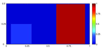
Near-wall and near-obstacle effects have a strong influence on the dynamics on constrained macroscopic evolutions. We propose that pedestrians take into account walls and obstacles in their computation of optimal paths. Hence it is natural to include these effects as an additional fixed cost $W(x)$ on the right-hand side of the eikonal equation (4). We introduce a smooth layer profile $\chi_{w}(x)\in[0,1]$, which identifies areas close to walls but smoothly vanishes elsewhere and around exits to allow outflow. A typical choice of $\chi_{w}$ is illustrated in Figure 1. For the sake of simplicity, we set

(10) $$W(x)=\frac{\chi_{w}(x)}{f(\rho_{\max}-\epsilon)},$$

hence areas close to walls are penalised similar to high density areas.

\psscalebox

.75 .75 exitwallwall$w$ $w$ $\chi_{w}$ $T_{1}$0000$T_{2}$0000$1$ $1$0000

Figure 1. Illustration of layer profile $\chi_{w}$: wall and obstacle repulsion are embedded to the model with a fixed cost $W$ defined in terms of the layer profile $\chi_{w}(x)\in[0,1]$, see (10), which indicates proximity to walls less than a width $w$, but vanishes away from obstacles and near exits to allow a proper outflow of pedestrians. $\chi_{w}$ equals one at walls and is the linear function given by vertex values within triangles $T_{1}$, $T_{2}$ near exits.

Finally all terms are coupled to the continuity equation with velocity field $v(x,t)=-f(\rho)\mathcal{P}[\nabla\varphi]$ as in the original model. At exits, we prescribe a maximum outflow, given by $v(\xi,t)=-f(\rho)\vec{n}$ for all $\xi\in\partial\Omega_{\text{exit}}$. Taking all these considerations into account the full macroscopic model reads as:

(11a) $$\displaystyle\partial_{t}\rho(x,t)+\nabla_{x}\cdot\left(-f(\rho(x,t))\mathcal{P}[\nabla\varphi(x,t)]\rho(x,t)\right)=0$$
(11b) $$\displaystyle\varphi(x,t)=\frac{(\rho u\star\mathcal{K})(x,t)}{(\rho\star\mathcal{K})(x,t)}$$
(11c) $$\displaystyle u(x,t)=\frac{\nabla_{y}\phi_{k^{\text{opt}}}(x,x,t)}{\|\nabla_{y}\phi_{k^{\text{opt}}}(x,x,t)\|}(\phi_{k^{\text{opt}+1}}(x,x,t)-\phi_{k^{\text{opt}}}(x,x,t))$$
(11d) $$\displaystyle k^{\text{opt}}(x,t)=\operatorname{argmin}\limits_{k}\phi_{k}(x,x,t)$$
(11e) $$\displaystyle k^{\text{opt+1}}(x,t)=\operatorname{argmin}\limits_{k\neq k^{\text{opt}}}\phi_{k}(x,x,t)$$
(11f) $$\displaystyle\|\nabla_{y}\phi_{k}(x,y,t)\|=\displaystyle{\begin{cases}\frac{1}{f(\rho(y,t)}+W(y)&y\in V_{x}\\[2.84526pt] \frac{1}{f(\rho_{H})}&y\in H_{x}\\ \end{cases}}$$
(11g) $$\displaystyle\text{s.t.:}\,\left.\phi_{k}\right|_{\partial\Omega_{E_{k}}}=0,k=1,\dots,M\,,\forall t$$
(11h) $$\displaystyle\text{s.t.:}\,\mathcal{P}[\varphi(\xi,t)]=\vec{n}\,,\,\,\forall\xi\in\partial\Omega_{\text{exit}}\,,\,\,\,\text{s.t.:}\,\rho(x,0)=\rho_{0}(x).$$

We conclude the section with remarks on specific modeling assumptions.

Remark (vision cones).

We have set aside formal statements regarding assumptions on the visible set $V_{x}$, but clearly we think of at least regular, connected and closed sets. A necessary condition is

(12) $$x\in V^{\circ}_{x}=\operatorname{int}V_{x},$$

which implies that every pedestrian perceives some information from all directions. This restriction rules out e.g. angular vision cones (see Degond et.al.[15]) where pedestrians do not see what is happening behind them. In our model, (12) is necessary to exclude unrealistic situations where the chosen walking direction points outside the visible area. The inclusion of angular-dependent vision cones is certainly possible, but would imply a velocity-dependency and lead towards a second-order macroscopic model.

Remark (conviction term).

The introduction of the conviction term $u(x)$ requires the computation of exit costs $\phi_{k}$ via the eikonal equation for individual exits, which appears to be a significant complication of the model. However, it is worth noting that the mechanism is almost identical to the original model. In equation (1b) the costs of walking towards any of the $K$ exits are compared, but only the minimal costs are used. Here, we simply store more information. This connection is also illustrated by looking at the numerical schemes for solving the eikonal equation (see also Section ?): If a Fast Sweeping Method is used in e.g. a corridor with two exists, this essentially corresponds to solving for each exit separately if the minimization step is left out. If a Fast Marching Method is used, the conviction is directly related to the sequence in which vertices are promoted, with the least convinced vertex being assigned a cost the latest.

Remark (waiting behavior).

The relaxation $\|\mathcal{P}[x]\|\leq 1$ implies that the modulus of the flux can be less than $f(\rho)\rho$ when pedestrians are undecided. This makes a rigorous analysis of the model equations a difficult task, which is not tackled in this work. The benefit of our formulation is that the problem of discontinuous velocity fields at sonic points has disappeared. Pedestrians at those hyper surfaces will not move unless the sonic points move.

3.2. The one-dimensional case

Consider a one-dimensional corridor $\Omega=[0,1]$ with two exits and the uniform radial vision cone $V_{x}=[x-L/2,x+L/2]\cap\Omega$ of length $L$. Exit costs towards the left and right exit are computed at $y\in V_{x}$ as

$$\displaystyle\phi_{L}(x,y,t)=\int\limits_{z<y,z\in H_{x}}\frac{1}{f(\rho_{H})}\mathrm{d}z+\int\limits_{z<y,z\in V_{x}}\frac{1}{f(\rho(z,t))}\mathrm{d}z,$$
$$\displaystyle\phi_{R}(x,y,t)=\int\limits_{z>y,z\in H_{x}}\frac{1}{f(\rho_{H})}\mathrm{d}z+\int\limits_{z>y,z\in V_{x}}\frac{1}{f(\rho(z,t))}\mathrm{d}z,$$
$$\displaystyle u(x,t)=\phi_{L}(x,x,t)-\phi_{R}(x,x,t),$$

as illustrated in Fig. 2.

\psscalebox

.75 .7500$x_{0}$ $1$ $V_{x_{0}}$ $\phi_{L}$ $\phi_{R}$ $|u(x_{0})|$

Figure 2. Illustration of path optimisation mechanism in 1D: A pedestrian located at $x_{0}$ computes and compares the cost potential $\phi_{L},\phi_{R}$ of left vs. right exit in a corridor $[0,1]$. Next to its own negligible density, the present crowd consists of three blocks. Outside the vision cone $V_{x}$, the evacuation costs grow linearly at constant rate, as the local density is unknown. Within $V_{x}$, the slope of the cost potential increases with the pedestrian density. Preference is then given towards the exit with lower estimated cost. The conviction towards this decision is given as the cost benefit $|u(x_{0})|=|\phi_{L}-\phi_{R}|$.

The cost potential $\phi$ is two-dimensional and $\partial_{y}\phi(x,y)$ gives the preferred walking direction that a pedestrian located at $x$ seeing $V_{x}$ assigns to $y\in[0,1]$. The walking directions chosen prior to the consensus process are hence given as $\partial_{y}\phi(x,x)$ along the diagonal of $[0,1]^{2}$. For every fixed $x\in[0,1]$, there is a unique sonic point $z(x)$, where $\phi_{L}(x,z(x))=\phi_{R}(x,z(x))$ and $\partial_{y}\phi(x,z(x))$ does not exist. As illustrated in Fig. 3, the individually preferred walking directions can switch multiple times between both exits, depending on the current density and the vision cones. At switching points, the preferred directions can point outwards (separation) or inwards (collision) and only the weighted interaction process (11b)-(11c) generates a smooth velocity profile. In the Hughes’ model, all vision cones are identical and there is a single separation point.

\psscalebox.9 .9 \psaxes[labelFontSize=,Ox=0,Oy=0,Dx=1,Dy=1]-(0,0)(0,0)(1,1) \savedata\mydata[ 0.423,0.00050.423,0.00150.422,0.00250.422,0.00350.422,0.0045 0.422,0.00550.422,0.00650.422,0.00750.422,0.00850.421,0.00950.421,0.0105 0.421,0.01150.421,0.01250.421,0.01350.421,0.01450.421,0.01550.421,0.0165 0.42,0.01750.42,0.01850.42,0.01950.42,0.02050.42,0.02150.42,0.0225 0.42,0.02350.42,0.02450.42,0.02550.42,0.02650.42,0.02750.42,0.0285 0.42,0.02950.42,0.03050.419,0.03150.419,0.03250.419,0.03350.419,0.0345 0.419,0.03550.419,0.03650.419,0.03750.419,0.03850.419,0.03950.419,0.0405 0.419,0.04150.419,0.04250.419,0.04350.419,0.04450.419,0.04550.419,0.0465 0.419,0.04750.419,0.04850.419,0.04950.419,0.05050.419,0.05150.419,0.0525 0.419,0.05350.419,0.05450.419,0.05550.419,0.05650.419,0.05750.419,0.0585 0.419,0.05950.419,0.06050.419,0.06150.419,0.06250.419,0.06350.419,0.0645 0.419,0.06550.419,0.06650.419,0.06750.419,0.06850.419,0.06950.419,0.0705 0.419,0.07150.419,0.07250.419,0.07350.419,0.07450.419,0.07550.419,0.0765 0.419,0.07750.419,0.07850.419,0.07950.419,0.08050.419,0.08150.419,0.0825 0.419,0.08350.419,0.08450.419,0.08550.419,0.08650.419,0.08750.419,0.0885 0.419,0.08950.419,0.09050.419,0.09150.419,0.09250.419,0.09350.419,0.0945 0.419,0.09550.419,0.09650.419,0.09750.419,0.09850.419,0.09950.419,0.1005 0.419,0.10150.419,0.10250.419,0.10350.419,0.10450.419,0.10550.419,0.1065 0.419,0.10750.419,0.10850.419,0.10950.419,0.11050.419,0.11150.419,0.1125 0.419,0.11350.419,0.11450.419,0.11550.419,0.11650.419,0.11750.419,0.1185 0.419,0.11950.419,0.12050.419,0.12150.419,0.12250.419,0.12350.419,0.1245 0.419,0.12550.419,0.12650.418,0.12750.418,0.12850.418,0.12950.418,0.1305 0.418,0.13150.418,0.13250.418,0.13350.418,0.13450.418,0.13550.418,0.1365 0.418,0.13750.418,0.13850.418,0.13950.418,0.14050.418,0.14150.418,0.1425 0.418,0.14350.418,0.14450.418,0.14550.417,0.14650.417,0.14750.417,0.1485 0.417,0.14950.417,0.15050.417,0.15150.417,0.15250.417,0.15350.417,0.1545 0.417,0.15550.417,0.15650.417,0.15750.417,0.15850.416,0.15950.416,0.1605 0.416,0.16150.416,0.16250.416,0.16350.416,0.16450.416,0.16550.416,0.1665 0.416,0.16750.416,0.16850.416,0.16950.416,0.17050.416,0.17150.417,0.1725 0.417,0.17350.417,0.17450.417,0.17550.417,0.17650.417,0.17750.417,0.1785 0.417,0.17950.417,0.18050.417,0.18150.417,0.18250.418,0.18350.418,0.1845 0.418,0.18550.418,0.18650.418,0.18750.418,0.18850.418,0.18950.418,0.1905 0.418,0.19150.419,0.19250.419,0.19350.419,0.19450.419,0.19550.419,0.1965 0.419,0.19750.419,0.19850.419,0.19950.419,0.20050.42,0.20150.42,0.2025 0.42,0.20350.42,0.20450.42,0.20550.42,0.20650.42,0.20750.42,0.2085 0.42,0.20950.421,0.21050.421,0.21150.421,0.21250.421,0.21350.421,0.2145 0.421,0.21550.421,0.21650.421,0.21750.422,0.21850.422,0.21950.422,0.2205 0.422,0.22150.422,0.22250.422,0.22350.422,0.22450.423,0.22550.423,0.2265 0.423,0.22750.423,0.22850.423,0.22950.423,0.23050.423,0.23150.423,0.2325 0.424,0.23350.424,0.23450.424,0.23550.424,0.23650.424,0.23750.424,0.2385 0.424,0.23950.425,0.24050.425,0.24150.425,0.24250.425,0.24350.425,0.2445 0.425,0.24550.425,0.24650.425,0.24750.425,0.24850.426,0.24950.426,0.2505 0.426,0.25150.426,0.25250.426,0.25350.426,0.25450.426,0.25550.427,0.2565 0.427,0.25750.427,0.25850.427,0.25950.427,0.26050.427,0.26150.428,0.2625 0.428,0.26350.428,0.26450.428,0.26550.428,0.26650.428,0.26750.429,0.2685 0.429,0.26950.429,0.27050.429,0.27150.429,0.27250.429,0.27350.43,0.2745 0.43,0.27550.43,0.27650.43,0.27750.43,0.27850.431,0.27950.431,0.2805 0.431,0.28150.431,0.28250.431,0.28350.432,0.28450.432,0.28550.432,0.2865 0.432,0.28750.433,0.28850.433,0.28950.433,0.29050.433,0.29150.433,0.2925 0.434,0.29350.434,0.29450.434,0.29550.434,0.29650.435,0.29750.435,0.2985 0.435,0.29950.435,0.30050.436,0.30150.436,0.30250.436,0.30350.436,0.3045 0.437,0.30550.437,0.30650.437,0.30750.437,0.30850.438,0.30950.438,0.3105 0.438,0.31150.438,0.31250.439,0.31350.439,0.31450.439,0.31550.44,0.3165 0.44,0.31750.44,0.31850.44,0.31950.441,0.32050.441,0.32150.441,0.3225 0.442,0.32350.442,0.32450.442,0.32550.442,0.32650.443,0.32750.443,0.3285 0.443,0.32950.444,0.33050.444,0.33150.444,0.33250.445,0.33350.445,0.3345 0.445,0.33550.446,0.33650.446,0.33750.446,0.33850.447,0.33950.447,0.3405 0.447,0.34150.448,0.34250.448,0.34350.448,0.34450.449,0.34550.449,0.3465 0.449,0.34750.45,0.34850.45,0.34950.45,0.35050.451,0.35150.451,0.3525 0.451,0.35350.452,0.35450.452,0.35550.453,0.35650.453,0.35750.453,0.3585 0.454,0.35950.454,0.36050.454,0.36150.455,0.36250.455,0.36350.456,0.3645 0.456,0.36550.456,0.36650.457,0.36750.457,0.36850.457,0.36950.458,0.3705 0.458,0.37150.459,0.37250.459,0.37350.459,0.37450.46,0.37550.46,0.3765 0.461,0.37750.461,0.37850.461,0.37950.462,0.38050.462,0.38150.462,0.3825 0.463,0.38350.463,0.38450.464,0.38550.464,0.38650.464,0.38750.465,0.3885 0.465,0.38950.466,0.39050.466,0.39150.466,0.39250.467,0.39350.467,0.3945 0.468,0.39550.468,0.39650.468,0.39750.469,0.39850.469,0.39950.469,0.4005 0.47,0.40150.47,0.40250.471,0.40350.471,0.40450.471,0.40550.472,0.4065 0.472,0.40750.472,0.40850.473,0.40950.473,0.41050.474,0.41150.474,0.4125 0.474,0.41350.475,0.41450.475,0.41550.475,0.41650.476,0.41750.476,0.4185 0.477,0.41950.477,0.42050.477,0.42150.478,0.42250.478,0.42350.478,0.4245 0.479,0.42550.479,0.42650.479,0.42750.48,0.42850.48,0.42950.48,0.4305 0.481,0.43150.481,0.43250.481,0.43350.482,0.43450.482,0.43550.482,0.4365 0.483,0.43750.483,0.43850.483,0.43950.484,0.44050.484,0.44150.484,0.4425 0.485,0.44350.485,0.44450.485,0.44550.486,0.44650.486,0.44750.486,0.4485 0.486,0.44950.487,0.45050.487,0.45150.487,0.45250.488,0.45350.488,0.4545 0.488,0.45550.488,0.45650.489,0.45750.489,0.45850.489,0.45950.489,0.4605 0.49,0.46150.49,0.46250.49,0.46350.49,0.46450.491,0.46550.491,0.4665 0.491,0.46750.491,0.46850.492,0.46950.492,0.47050.492,0.47150.492,0.4725 0.492,0.47350.493,0.47450.493,0.47550.493,0.47650.493,0.47750.494,0.4785 0.494,0.47950.494,0.48050.494,0.48150.494,0.48250.494,0.48350.495,0.4845 0.495,0.48550.495,0.48650.495,0.48750.495,0.48850.496,0.48950.496,0.4905 0.496,0.49150.496,0.49250.496,0.49350.496,0.49450.497,0.49550.497,0.4965 0.497,0.49750.497,0.49850.497,0.49950.497,0.50050.497,0.50150.498,0.5025 0.498,0.50350.498,0.50450.498,0.50550.498,0.50650.498,0.50750.498,0.5085 0.498,0.50950.498,0.51050.499,0.51150.499,0.51250.499,0.51350.499,0.5145 0.499,0.51550.499,0.51650.499,0.51750.499,0.51850.499,0.51950.499,0.5205 0.499,0.52150.499,0.52250.499,0.52350.5,0.52450.5,0.52550.5,0.5265 0.5,0.52750.5,0.52850.5,0.52950.5,0.53050.5,0.53150.5,0.5325 0.5,0.53350.5,0.53450.5,0.53550.5,0.53650.5,0.53750.5,0.5385 0.5,0.53950.5,0.54050.5,0.54150.5,0.54250.5,0.54350.5,0.5445 0.5,0.54550.5,0.54650.5,0.54750.5,0.54850.5,0.54950.5,0.5505 0.501,0.55150.501,0.55250.501,0.55350.502,0.55450.502,0.55550.503,0.5565 0.503,0.55750.504,0.55850.505,0.55950.505,0.56050.506,0.56150.506,0.5625 0.507,0.56350.508,0.56450.509,0.56550.51,0.56650.51,0.56750.511,0.5685 0.512,0.56950.513,0.57050.514,0.57150.515,0.57250.516,0.57350.517,0.5745 0.518,0.57550.519,0.57650.52,0.57750.522,0.57850.523,0.57950.524,0.5805 0.525,0.58150.527,0.58250.528,0.58350.53,0.58450.531,0.58550.532,0.5865 0.534,0.58750.536,0.58850.537,0.58950.539,0.59050.54,0.59150.542,0.5925 0.544,0.59350.546,0.59450.548,0.59550.549,0.59650.551,0.59750.553,0.5985 0.555,0.59950.557,0.60050.56,0.60150.562,0.60250.564,0.60350.565,0.6045 0.566,0.60550.569,0.60650.571,0.60750.574,0.60850.576,0.60950.579,0.6105 0.582,0.61150.584,0.61250.587,0.61350.59,0.61450.593,0.61550.596,0.6165 0.599,0.61750.603,0.61850.606,0.61950.609,0.62050.613,0.62150.616,0.6225 0.62,0.62350.623,0.62450.627,0.62550.631,0.62650.634,0.62750.638,0.6285 0.642,0.62950.647,0.63050.651,0.63150.655,0.63250.659,0.63350.664,0.6345 0.668,0.63550.672,0.63650.677,0.63750.681,0.63850.686,0.63950.69,0.6405 0.695,0.64150.699,0.64250.704,0.64350.708,0.64450.713,0.64550.717,0.6465 0.722,0.64750.726,0.64850.731,0.64950.735,0.65050.74,0.65150.745,0.6525 0.749,0.65350.754,0.65450.758,0.65550.763,0.65650.767,0.65750.772,0.6585 0.776,0.65950.781,0.66050.785,0.66150.79,0.66250.794,0.66350.798,0.6645 0.801,0.66550.804,0.66650.806,0.66750.808,0.66850.809,0.66950.811,0.6705 0.812,0.67150.814,0.67250.815,0.67350.816,0.67450.818,0.67550.819,0.6765 0.82,0.67750.821,0.67850.822,0.67950.823,0.68050.824,0.68150.825,0.6825 0.826,0.68350.827,0.68450.828,0.68550.828,0.68650.829,0.68750.83,0.6885 0.831,0.68950.832,0.69050.832,0.69150.833,0.69250.834,0.69350.834,0.6945 0.835,0.69550.836,0.69650.836,0.69750.837,0.69850.837,0.69950.838,0.7005 0.838,0.70150.839,0.70250.839,0.70350.84,0.70450.84,0.70550.841,0.7065 0.841,0.70750.842,0.70850.842,0.70950.842,0.71050.843,0.71150.843,0.7125 0.844,0.71350.844,0.71450.844,0.71550.845,0.71650.845,0.71750.845,0.7185 0.846,0.71950.846,0.72050.846,0.72150.847,0.72250.847,0.72350.847,0.7245 0.847,0.72550.848,0.72650.848,0.72750.848,0.72850.848,0.72950.849,0.7305 0.849,0.73150.849,0.73250.849,0.73350.849,0.73450.85,0.73550.85,0.7365 0.85,0.73750.85,0.73850.85,0.73950.85,0.74050.851,0.74150.851,0.7425 0.851,0.74350.851,0.74450.851,0.74550.851,0.74650.851,0.74750.851,0.7485 0.851,0.74950.851,0.75050.851,0.75150.852,0.75250.852,0.75350.852,0.7545 0.852,0.75550.852,0.75650.852,0.75750.852,0.75850.852,0.75950.852,0.7605 0.852,0.76150.852,0.76250.852,0.76350.852,0.76450.852,0.76550.852,0.7665 0.852,0.76750.852,0.76850.852,0.76950.852,0.77050.852,0.77150.852,0.7725 0.852,0.77350.852,0.77450.852,0.77550.852,0.77650.852,0.77750.852,0.7785 0.852,0.77950.852,0.78050.852,0.78150.852,0.78250.852,0.78350.852,0.7845 0.852,0.78550.852,0.78650.852,0.78750.852,0.78850.852,0.78950.852,0.7905 0.852,0.79150.853,0.79250.853,0.79350.853,0.79450.853,0.79550.853,0.7965 0.853,0.79750.853,0.79850.853,0.79950.853,0.80050.853,0.80150.853,0.8025 0.853,0.80350.853,0.80450.853,0.80550.853,0.80650.853,0.80750.853,0.8085 0.853,0.80950.853,0.81050.853,0.81150.853,0.81250.853,0.81350.853,0.8145 0.853,0.81550.853,0.81650.853,0.81750.853,0.81850.853,0.81950.853,0.8205 0.853,0.82150.853,0.82250.853,0.82350.853,0.82450.853,0.82550.853,0.8265 0.853,0.82750.853,0.82850.853,0.82950.853,0.83050.853,0.83150.853,0.8325 0.853,0.83350.853,0.83450.853,0.83550.853,0.83650.853,0.83750.853,0.8385 0.853,0.83950.853,0.84050.853,0.84150.853,0.84250.853,0.84350.853,0.8445 0.853,0.84550.853,0.84650.853,0.84750.853,0.84850.854,0.84950.854,0.8505 0.854,0.85150.854,0.85250.854,0.85350.854,0.85450.854,0.85550.854,0.8565 0.854,0.85750.854,0.85850.854,0.85950.854,0.86050.854,0.86150.854,0.8625 0.854,0.86350.854,0.86450.854,0.86550.854,0.86650.854,0.86750.854,0.8685 0.854,0.86950.854,0.87050.854,0.87150.854,0.87250.854,0.87350.854,0.8745 0.854,0.87550.854,0.87650.854,0.87750.854,0.87850.854,0.87950.854,0.8805 0.854,0.88150.854,0.88250.854,0.88350.854,0.88450.854,0.88550.854,0.8865 0.854,0.88750.854,0.88850.854,0.88950.854,0.89050.854,0.89150.854,0.8925 0.854,0.89350.854,0.89450.854,0.89550.854,0.89650.854,0.89750.854,0.8985 0.854,0.89950.854,0.90050.854,0.90150.854,0.90250.854,0.90350.854,0.9045 0.854,0.90550.854,0.90650.854,0.90750.854,0.90850.854,0.90950.854,0.9105 0.854,0.91150.854,0.91250.854,0.91350.854,0.91450.854,0.91550.854,0.9165 0.854,0.91750.854,0.91850.854,0.91950.854,0.92050.854,0.92150.854,0.9225 0.854,0.92350.854,0.92450.854,0.92550.854,0.92650.854,0.92750.854,0.9285 0.854,0.92950.854,0.93050.854,0.93150.854,0.93250.854,0.93350.854,0.9345 0.854,0.93550.854,0.93650.854,0.93750.854,0.93850.854,0.93950.854,0.9405 0.854,0.94150.854,0.94250.854,0.94350.854,0.94450.854,0.94550.854,0.9465 0.854,0.94750.854,0.94850.854,0.94950.854,0.95050.854,0.95150.854,0.9525 0.854,0.95350.854,0.95450.854,0.95550.854,0.95650.854,0.95750.854,0.9585 0.854,0.95950.854,0.96050.854,0.96150.854,0.96250.854,0.96350.854,0.9645 0.854,0.96550.854,0.96650.854,0.96750.854,0.96850.854,0.96950.854,0.9705 0.854,0.97150.854,0.97250.854,0.97350.854,0.97450.854,0.97550.854,0.9765 0.854,0.97750.854,0.97850.854,0.97950.854,0.98050.854,0.98150.854,0.9825 0.854,0.98350.854,0.98450.854,0.98550.854,0.98650.854,0.98750.854,0.9885 0.854,0.98950.854,0.99050.854,0.99150.854,0.99250.854,0.99350.854,0.9945 0.854,0.99550.854,0.99650.854,0.99750.854,0.9985,0.854,0.9995 ] $y$ $x$ $z(x)$\dataplot[plotstyle=line,linestyle=solid,linecolor=blue,linewidth=0.04]\mydata \psscalebox.9 .9 \psaxes[labelFontSize=,Ox=0,Oy=0,Dx=1,Dy=1]-(0,0)(0,0)(1,1) $y$ $x$ $z(x)$
(a) Localized model (b) Hughes’ model
Figure 3. Illustration of turning decisions of a 1D population for a given $\rho(x,t)$: For every point $x,$ we show the individual sonic point $z(x)$, where the costs $\phi_{L}(x,z(x))=\phi_{R}(x,z(x))$ coincide. The preferred walking direction for a pedestrian at $x$ is found along the diagonal $(x,x)$. If the sonic point is to the left, the pedestrians aim to walk towards the right and vice-versa. No direction is preferred and the conviction is zero if the curve of sonic points intersects the diagonal. (a) Local vision cones: The preferred direction alters and creates multiple points of separation and collision. The resulting velocity field is obtained by the smoothening interaction process (11b)-(11c) . (b) Hughes’ model: All vision cones coincide, hence there is one identical sonic point common to all pedestrians.

3.3. Microscopic interpretation

We conclude this section by briefly commenting on the modelling of local vision at the microscopic level. The microscopic modification is straightforward and uses the same ideas as at the macroscopic level. It corresponds to updating the position $X=X(t)$ according to a potential which depends on local information only. Its calculation is based on the same equations as in the macroscopic model (11f) but using the smoothed empirical density $\rho^{N}_{g}$ instead of $\rho$. The position update is based on equations (11b)-(11e). Hence individuals choose the path towards the exit with the lowest cost, but weigh their decision according to the predominant direction chosen around them. For further details on the implementation we refer to Algorithm 2 presented in Section 4.

3.4. Analysis of the domains of dependence

In this subsection, we will discuss some mathematical properties of the solutions of the eikonal equations (11f). From the construction of the model, the potential $\phi(x,y,t)$ has to be computed for every $x\in\Omega$ on the entire domain $\Omega$, which counterbalances the idea of locality and increases the computational cost considerably. We show here, that the computation of the potential can actually be reduced to a subset of $\Omega$, called the effective domain of dependence, for every $x$. Only this subset, which contains $V_{x}$, is considered in the individual local planning problem and corresponds to the reduction of the computational cost.

The following proofs rely crucially on the optimal path property of the characteristics associated to the eikonal equation (11f). We recall[24, 4] that by Fermat’s principle the characteristic paths associated to $\phi(x,y,t)$, given by the solution of:

(13) $$\gamma_{x,t}^{z}(s)\subset\Omega:\gamma(0)=z,\dot{\gamma}(s)=-\nabla\phi(x,\gamma(s),t)\,\,\mbox{ for all}\,s\geq 0\,,$$

are the optimal paths for the cost defined as

$$c(y,t)=\displaystyle{\begin{cases}\frac{1}{f(\rho(y,t))}+W(y)&y\in V_{x}\\[2.84526pt] \frac{1}{f(\rho_{H})}&y\in H_{x}\\ \end{cases}}\,.$$

Moreover, the potential is the value function for that cost. Hence it is decreasing along these paths and satisfies the optimality condition

(14) $$\phi(x,\gamma_{x,t}^{z}(a),t)-\phi(x,\gamma_{x,t}^{z}(b),t)=\int_{a}^{b}c(\gamma_{x,t}^{z}(s),t)\,ds\,,\mbox{ for all }0\leq a<b\,,$$

being zero at its corresponding exit $\partial\Omega_{\text{exit}}$. Furthermore, the curves $\gamma_{x,t}^{z}$ are the optimal paths to achieve the exit, i.e., they verify the following global optimality condition

(15) $$+\phi(x,z,t)=\int_{0}^{T_{z}}c(\gamma_{x,t}^{z}(s),t)\,ds\leq\int_{0}^{\tilde{T}_{z}}c(\tilde{\gamma}(s),t)\,ds\,,$$

for all $\tilde{\gamma}$ curves joining $z$ to any point in the exit $\partial\Omega_{\text{exit}}$, where $T_{z}$ is the optimal time to achieve the exit for the point $z\in\Omega$ and $\tilde{T}_{z}$ is the time to achieve the exit for the path $\tilde{\gamma}$.

Lemma 1.

Consider any fixed $V_{x}\subset\Omega$ and that $f(\rho)>0$, $0\leq\rho<\rho_{\max}$. Let $\phi_{H}$ be the global solution of the eikonal equation $\|\nabla\phi_{H}\|=1/f(\rho_{H}),\phi_{H}(x)=0\text{ on }\partial\Omega_{\text{exit}}$. Define the minimum of $\phi_{H}$ in $V_{x}$ as

$$m_{H}:=\min_{z\in V_{x}}\phi_{H}(z)$$

and the corresponding superlevel set of $\phi_{H}$ as

$$M_{H}:=\{x\in\Omega:\phi_{H}(x)\geq m_{\phi}\}.$$

Then the problem of computing the local potential $\phi(x,y,t)=:\tilde{\phi}(y)$ out of (11f) on $\Omega$ reduces to the following problem on $M_{\phi}$:

$$\begin{cases}\|\nabla_{y}\tilde{\phi}(y)\|=\frac{1}{f(\rho(y,t))}+W(y)&\text{ in }V_{x}\\ \|\nabla_{y}\tilde{\phi}(y)\|=\frac{1}{f(\rho_{H})}&\text{ in }M_{H}\backslash V_{x}\\ \tilde{\phi}(y)=m_{H}&\text{ on }\partial M_{H}\backslash\partial\Omega_{\text{wall}}\,\,(\text{B.C. })\end{cases}\,.$$
Proof.

If an exit is visible then $m_{H}=0,M_{H}=\Omega$ and the assertion is trivial. If no exit is visible then by construction $V_{x}\subset M_{H}$ and $\phi_{H}=m_{H}>0$ on $\partial M_{H}$. As the walking costs are always positive, $c(y,t)>0$, we get $\phi(x,y,t)>m_{H}$ for all $y\in\operatorname{int}M_{H}$. On the other hand, any point $z\in\Omega\backslash M_{H}$ satisfies $\phi(x,z,t)<m_{H}$ and hence $\gamma_{x,t}^{z}(s)$ does not intersect $V_{x}$, otherwise the cost should be larger at a middle point than initially contradicting the optimality of the path $\gamma_{x,t}^{z}(s)$ in (14). Hence $\partial M_{H}$ is the maximal level set consisting of points whose optimal paths do not cross $V_{x}$, and therefore, $\phi(x,z,t)$ can be computed from (11f) with constant right-hand side outside $M_{H}$. ∎

Definition 1.

Consider a fixed visibility area $V_{x}$. For a $z\in\Omega$, denote the default optimal path $\gamma_{H}^{z}$ as the parameterised curve associated to a gradient walk along $\phi_{H}$ starting in $z$, that is

$$\gamma_{H}^{z}(s)\subset\Omega:\gamma(0)=z,\dot{\gamma}(s)=-\nabla\phi_{H}(\gamma(s))\,\,\forall\,s\geq 0.$$

Next, define the characteristics’ shadow $V^{\#}$ as the set of all points, whose default optimal paths crosses the visibility area, hence

$$V^{\#}:=\{z\in\Omega:\gamma_{H}^{z}\cap\operatorname{int}V_{x}\neq\emptyset\}.$$

Note, that $V^{\#}\subset M_{H}$ since any default optimal path outside of $M_{H}$ cannot intersect with $V_{x}$ as proven in the previous lemma.

Lemma 2.

Consider any fixed $V_{x}\subset\Omega$ and assume that $f(\rho)>0$ is increasing in $0\leq\rho<\rho_{\max}$, with $\rho_{H}=0$, then the problem of computing the local potential $\tilde{\phi}(y)$ out of (4) further reduces to the following problem on $V^{\#}$

$$\begin{cases}\|\nabla_{y}\tilde{\phi}(y)\|=\frac{1}{f(\rho(y,t))}+W(y)&\text{ in }V_{x}\\ \|\nabla_{y}\tilde{\phi}(y)\|=\frac{1}{f(0)}&\text{ in }V^{\#}\backslash V_{x}\\ \tilde{\phi}\equiv\phi_{H}&\text{ on }\partial V^{\#}\end{cases}\,.$$
Proof.

For any point $z$ whose default optimal path $\gamma_{H}^{z}$ that does not intersect with $V$, the claim is that $\tilde{\phi}(z)=\phi_{H}(z)$ due the monotonicity of the cost function, i.e.,

$$\frac{1}{f(\rho(y,t))}+W(y)\geq\frac{1}{f(0)}\,.$$

To prove this, let us denote by $T_{z}^{H}$ the optimal time to get to the exit for the default optimal path $\gamma_{H}^{z}$.

We first take $\gamma_{x,t}^{z}(s)$ as a candidate path in the global optimality condition (15) for the eikonal equation with right hand side $c_{H}=\tfrac{1}{f(0)}$. Being $\gamma_{x,t}^{z}(s)$ a path joining $z$ to a point in the exit and $\gamma_{H}^{z}(s)$ the optimal one, we conclude

$$\phi_{H}(z)=T_{z}^{H}c_{H}\leq T_{z}c_{H}\leq\int_{0}^{T_{z}}c(\gamma_{x,t}^{z}(s),t)\,ds=\tilde{\phi}(z)\,.$$

Now, we take $\gamma_{H}(z)$ as a candidate path in the global optimality condition (15) for the eikonal equation with right hand side $c(y,t)$. It is an admissible path as it connects $z$ to a point at the exit and the cost along its path coincides with $c_{H}=c(\gamma_{H}^{z}(s),t)$ for all $s\in[0,T_{Z}^{H}]$ since the path does not cross $V$. Then, we get

$$\tilde{\phi}(z)\leq\int_{0}^{T_{z}^{H}}c(\gamma_{H}^{z}(s),t)\,ds=T_{z}^{H}c_{H}=\phi_{H}(z)\,,$$

leading to the stated result. ∎

\psscalebox

1 1 $V$ $V^{\#}$ $M_{H}$

Figure 4. Illustration of the domains $V,M_{H}$ and $V^{\#}$ for computation of the visibility area potential $\tilde{\phi}$ for the case of a corridor with two opposing exits: The problem on $\Omega$ generally reduces to a HJ-equation on $M_{H}$, as by construction $\tilde{\phi}$ coincides with $\phi_{H}$ outside of $M_{H}$ (Lemma (1), $-\nabla\phi_{H}$ solid arrows). If $\rho_{H}=0$, any default optimal path of $\phi_{H}$ that does not intersect $V$ remains optimal, as indicated by dotted arrows, and the problem reduces to $V^{\#}$ (Lemma 2).

We illustrate Lemmata 1 and 2 in Figure 4. It can be seen, that the reduction of the computational domain from $M_{H}$ to $V^{\#}$ can be significant, as the size of $M_{H}$ depends on the closeness of $V$ to the nearest exit, not on the size of $V$. For the exemplary geometry of Figure 4, the boundary of $V^{\#}$ coincides with the sonic points of $\phi_{H}$, but this is not true in general. Furthermore, it is easy to see why the computational domain cannot be reduced further. Suppose that $\rho(\cdot,t)$ is spatially homogeneous, then $-\nabla\phi$ in $V^{\#}\backslash V$ points to the left exit as in the eikonal case. On the other side, one can choose a situation with a large density at the left boundary of $V$ that leads to right-pointing $-\nabla\phi$ in $V^{\#}\backslash V$.

4. Computational methods

In this section we present a microscopic and a macroscopic numerical solver to simulate the classic and the local version of the Hughes model. The proposed methods have been implemented on regular and triangular meshes in 2D to allow for flexible discretizations of polygonal domains with one or several obstacles.

For the macroscopic system (11) we use the following explicit iterative algorithm:

Algorithm 1 Macroscopic version of the localised model

Initialisation:

  • A discretisation $\hat{\Omega}=(\mathcal{V},\mathcal{E},\mathcal{T})$ of $\Omega$ consisting of vertices, edges and cells.

  • An initial density $\hat{\rho}_{0}$ given on $\mathcal{T}$, such that $\int_{T}\rho(x,0)\mathrm{d}x=\hat{\rho}_{0}(T)\,\,\forall\,T\in\mathcal{T}$.

  • A list of exits, a list of boundary edges per exit and $|\mathcal{V}|$ subsets of $\mathcal{V}$ containing the vision cones defined in terms of vertices.

  1. (1)

    Compute the cost potential $\hat{\phi}_{k}$ for all exits out of the current density $\hat{\rho}$ by solving (11f) along the vertices for every $v\in\mathcal{V}$.

  2. (2)

    Determine the cell values of $\hat{\phi}_{k}$ and $\nabla\hat{\phi}_{k}$ by an averaging / finite difference approximation of the values at neighbouring vertices, e.g. $\hat{\phi}_{k}(T)=\frac{1}{|\{v\in\partial T\}|}\sum_{v\in\partial T}\hat{\phi}_{k}(u)$, and obtain $\hat{u}(T)$ here from.

  3. (3)

    Compute a numerical convolution of $\hat{u}$ with $\mathcal{K}$, which gives $\hat{\varphi}$ on the cells.

  4. (4)

    Update the density with a cell-based Finite Volume Method using the velocity field $-f(\hat{\rho})\mathcal{P}[\hat{\varphi}]$ and a suitably chosen time step.

The discretisation is either a regular grid or an unstructured regular triangular mesh to allow more complex geometries. For solving the eikonal equations, one can chose between Fast Sweeping Methods[38, 32] and Fast Marching Methods[28, 34]. The former is based on a Gauss-Seidel iteration, which updates the solution by passing through the computational domain in alternate pre-defined sweeping directions. A rectangular grid provides a natural ordering of all grid points. This ordering does not exist on an unstructured grid and is replaced by a general ordering strategy by introducing reference points, which is done once. Then the solution at each node is consecutively updated by running through the ordered lists. Marching methods update vertices in a monotone increasing order, where in every iteration a list of candidate values is available by finite difference approximation from previously approved values. The smallest value all of candidate values is then promoted and assigned to its vertex.

As a Finite Volume Method we use the first-order monotone FORCE scheme[35, 19]. Some postprocessing between the steps of Algorithm 1 is required: outward-pointing components of $\nabla\hat{\phi}_{k}$ are removed along the boundary, suitable values of $\nabla\hat{\phi}_{k}$ are ensured at corners of $\Omega$, and the max outflow condition (11h) is enforced at cells neighbouring exit edges.

The analogous algorithm used for the numerical simulation of the microscopic model is:

Algorithm 2 Microscopic version of the localised model

Let us consider a system of $N$ particles, which are initially located at positions $X^{j}(0)=X^{j}_{0}$. In every time step $t^{i}=i\Delta t$ we update the particle position as follows:

  1. (1)

    Determine the empirical density at time $t^{i}$:

    $\displaystyle\rho^{N}_{g}(x,t^{i})=\frac{1}{N}\sum_{j=1}^{N}g(x-X^{j}(t^{i})),$

    where $g$ denotes a Gaussian.

  2. (2)

    Solve the eikonal equation to determine the weighted distance to each exit $\phi^{k}=\phi^{k}(x,t^{i})$, $k=1,\ldots M$:

    (16a) $\displaystyle\|\nabla\phi^{k}(x,y,t^{i})\|$ $\displaystyle=\begin{cases}\frac{1}{f(\rho^{N}_{g}(y,t^{i}))}+W(y)&\text{ if }y\in V_{x}\\ \frac{1}{f(\rho_{H})}&\text{ otherwise.}\end{cases}$
    (16b) $\displaystyle\phi^{k}(x,t^{i})$ $\displaystyle=0$
  3. (3)

    Update the position of each particle $X^{j}$ via:

    (17) $\displaystyle\dot{X^{j}}(t^{i})=-f^{2}(\rho^{N}_{g}(x,t^{i})\cdot\nabla\varphi(x,t^{i}))),$

    where $\varphi(x,t^{i})$ is determined by (11b).

5. Results

In this section we illustrate the dynamics of the localised model for crowd dynamics with examples in one and two dimensions. In all simulations we consider an evacuation scenario of a corridor, where a given initial distribution of people tries to leave the rectangular domain through either one of the two exits as fast as possible. We compare the evacuation time, i.e. the time at which all individuals have left the domain, with respect to different parameters, e.g. vision cones. In the case of a global vision cone we obtain Hughes’ type dynamics. As a flux law, we chose the LWR function

(18) $$f(\rho)=\rho(1-\rho),$$

setting $\rho_{\max}=1$ throughout this section.

5.1. 1D corridor - macroscopic model

In our first example the domain $\Omega$ corresponds to the unit interval $\Omega=[0,1]$ with two exits located at either end, i.e. at $x=0$ and $x=1$. We consider an evacuation scenario in which two groups, one of them being densly packed, want to leave through either one of the exits:

(19) $$\rho_{0}(x)=\begin{cases}0.85&0\geq x\geq 0.3\\ 0&0.3<x<0.6\\ 0.25&0.6\geq x\geq 1\end{cases},$$

and we set the width of the vision cone to $L=0.75$. The resulting dynamics are illustrated at 4 time steps in Fig. 5. Within the left block, some pedestrians decide to walk towards the right exit, as they are aware of the high density on their left and account for a higher walking cost compared to the relatively empty right hand side. After the separation the right-moving part evolves as a rarefaction wave, as known from the LWR model. As the distance between the wave and the left-moving shock grows, the effects of the local vision cone become apparent. At some point pedestrians moving to the right do not see the high density at the left exit anymore and start to turn around. Therefore the rarefaction wave splits again - one part continues while the other one turns around and moves back to the left exit. The turn-around occurs in several stages:

  1. (1)

    A new sonic point arises, where pedestrians are undecided between both exits. The walking direction is unchanged as the local consensus process (11b) prevents an immediate switching.

  2. (2)

    When a critical mass of density and conviction opting for walking to the left, the velocity after consensus switches continuously and passing through zero. This creates a temporary collision point, as there a still pedestrians to the left of the sonic point which walk towards the right.

  3. (3)

    The density at the collision point increases, which causes pedestrians to the left of the collision point to turn around too, as a higher density is in their way, as it can bee seen in Fig. 5(c).

  4. (4)

    Finally, all pedestrians to the left of the initial sonic point have turned and walk towards the left ( Fig. 5(d)).

\psscalebox.9 .9 \psaxes[labelFontSize=,Ox=0,Oy=-1.0,Dx=0.25,Dy=0.5,ticksize=5pt,linecolor=lightgray]-(0,-1.0)(0,-1)(1,1) \savedata\mydata[ 0.0005,-10.0015,-10.0025,-10.0035,-10.0045,-1 0.0055,-10.0065,-10.0075,-10.0085,-10.0095,-10.0105,-1 0.0115,-10.0125,-10.0135,-10.0145,-10.0155,-10.0165,-1 0.0175,-10.0185,-10.0195,-10.0205,-10.0215,-10.0225,-1 0.0235,-10.0245,-10.0255,-10.0265,-10.0275,-10.0285,-1 0.0295,-10.0305,-10.0315,-10.0325,-10.0335,-10.0345,-1 0.0355,-10.0365,-10.0375,-10.0385,-10.0395,-10.0405,-1 0.0415,-10.0425,-10.0435,-10.0445,-10.0455,-10.0465,-1 0.0475,-10.0485,-10.0495,-10.0505,-10.0515,-10.0525,-1 0.0535,-10.0545,-10.0555,-10.0565,-10.0575,-10.0585,-1 0.0595,-10.0605,-10.0615,-10.0625,-10.0635,-10.0645,-1 0.0655,-10.0665,-10.0675,-10.0685,-10.0695,-10.0705,-1 0.0715,-10.0725,-10.0735,-10.0745,-10.0755,-10.0765,-1 0.0775,-10.0785,-10.0795,-10.0805,-10.0815,-10.0825,-1 0.0835,-10.0845,-10.0855,-10.0865,-10.0875,-10.0885,-1 0.0895,-10.0905,-10.0915,-10.0925,-10.0935,-10.0945,-1 0.0955,-10.0965,-10.0975,-10.0985,-10.0995,-10.1005,-1 0.1015,-10.1025,-10.1035,-10.1045,-10.1055,-10.1065,-1 0.1075,-10.1085,-10.1095,-10.1105,-10.1115,-10.1125,-1 0.1135,-10.1145,-10.1155,-10.1165,-10.1175,-10.1185,-1 0.1195,-10.1205,-10.1215,-10.1225,-10.1235,-10.1245,-1 0.1255,-10.1265,-10.1275,-10.1285,-10.1295,-10.1305,-1 0.1315,-10.1325,-10.1335,-10.1345,-10.1355,-10.1365,-1 0.1375,-10.1385,-10.1395,-10.1405,-10.1415,-10.1425,-1 0.1435,-10.1445,-10.1455,-10.1465,-10.1475,-10.1485,-1 0.1495,-10.1505,-10.1515,-10.1525,-10.1535,-10.1545,-1 0.1555,-10.1565,-10.1575,-10.1585,-10.1595,-10.1605,-1 0.1615,-10.1625,-10.1635,-10.1645,-10.1655,-10.1665,-1 0.1675,-10.1685,-10.1695,-10.1705,-10.1715,-10.1725,-1 0.1735,-10.1745,-10.1755,-10.1765,-10.1775,-10.1785,-1 0.1795,-10.1805,-10.1815,-10.1825,-10.1835,-10.1845,-1 0.1855,-10.1865,-10.1875,-10.1885,-10.1895,-10.1905,-1 0.1915,-10.1925,-10.1935,-10.1945,-10.1955,-10.1965,-1 0.1975,-10.1985,-10.1995,-10.2005,-10.2015,-10.2025,-1 0.2035,-10.2045,-10.2055,-10.2065,-10.2075,-10.2085,-1 0.2095,-10.2105,-10.2115,-10.2125,-10.2135,-10.2145,-1 0.2155,-10.2165,-10.2175,-10.2185,-10.2195,-10.2205,-1 0.2215,-10.2225,-10.2235,0.50.2245,10.2255,10.2265,1 0.2275,10.2285,10.2295,10.2305,10.2315,10.2325,1 0.2335,10.2345,10.2355,10.2365,10.2375,10.2385,1 0.2395,10.2405,10.2415,10.2425,10.2435,10.2445,1 0.2455,10.2465,10.2475,10.2485,10.2495,10.2505,1 0.2515,10.2525,10.2535,10.2545,10.2555,10.2565,1 0.2575,10.2585,10.2595,10.2605,10.2615,10.2625,1 0.2635,10.2645,10.2655,10.2665,10.2675,10.2685,1 0.2695,10.2705,10.2715,10.2725,10.2735,10.2745,1 0.2755,10.2765,10.2775,10.2785,10.2795,10.2805,1 0.2815,10.2825,10.2835,10.2845,10.2855,10.2865,1 0.2875,10.2885,10.2895,10.2905,10.2915,10.2925,1 0.2935,10.2945,10.2955,10.2965,10.2975,10.2985,1 0.2995,10.3005,10.3015,10.3025,10.3035,10.3045,1 0.3055,10.3065,10.3075,10.3085,10.3095,10.3105,1 0.3115,10.3125,10.3135,10.3145,10.3155,10.3165,1 0.3175,10.3185,10.3195,10.3205,10.3215,10.3225,1 0.3235,10.3245,10.3255,10.3265,10.3275,10.3285,1 0.3295,10.3305,10.3315,10.3325,10.3335,10.3345,1 0.3355,10.3365,10.3375,10.3385,10.3395,10.3405,1 0.3415,10.3425,10.3435,10.3445,10.3455,10.3465,1 0.3475,10.3485,10.3495,10.3505,10.3515,10.3525,1 0.3535,10.3545,10.3555,10.3565,10.3575,10.3585,1 0.3595,10.3605,10.3615,10.3625,10.3635,10.3645,1 0.3655,10.3665,10.3675,10.3685,10.3695,10.3705,1 0.3715,10.3725,10.3735,10.3745,10.3755,10.3765,1 0.3775,10.3785,10.3795,10.3805,10.3815,10.3825,1 0.3835,10.3845,10.3855,10.3865,10.3875,10.3885,1 0.3895,10.3905,10.3915,10.3925,10.3935,10.3945,1 0.3955,10.3965,10.3975,10.3985,10.3995,10.4005,1 0.4015,10.4025,10.4035,10.4045,10.4055,10.4065,1 0.4075,10.4085,10.4095,10.4105,10.4115,10.4125,1 0.4135,10.4145,10.4155,10.4165,10.4175,10.4185,1 0.4195,10.4205,10.4215,10.4225,10.4235,10.4245,1 0.4255,10.4265,10.4275,10.4285,10.4295,10.4305,1 0.4315,10.4325,10.4335,10.4345,10.4355,10.4365,1 0.4375,10.4385,10.4395,10.4405,10.4415,10.4425,1 0.4435,10.4445,10.4455,10.4465,10.4475,10.4485,1 0.4495,10.4505,10.4515,10.4525,10.4535,10.4545,1 0.4555,10.4565,10.4575,10.4585,10.4595,10.4605,1 0.4615,10.4625,10.4635,10.4645,10.4655,10.4665,1 0.4675,10.4685,10.4695,10.4705,10.4715,10.4725,1 0.4735,10.4745,10.4755,10.4765,10.4775,10.4785,1 0.4795,10.4805,10.4815,10.4825,10.4835,10.4845,1 0.4855,10.4865,10.4875,10.4885,10.4895,10.4905,1 0.4915,10.4925,10.4935,10.4945,10.4955,10.4965,1 0.4975,10.4985,10.4995,10.5005,10.5015,10.5025,1 0.5035,10.5045,10.5055,10.5065,10.5075,10.5085,1 0.5095,10.5105,10.5115,10.5125,10.5135,10.5145,1 0.5155,10.5165,10.5175,10.5185,10.5195,10.5205,1 0.5215,10.5225,10.5235,10.5245,10.5255,10.5265,1 0.5275,10.5285,10.5295,10.5305,10.5315,10.5325,1 0.5335,10.5345,10.5355,10.5365,10.5375,10.5385,1 0.5395,10.5405,10.5415,10.5425,10.5435,10.5445,1 0.5455,10.5465,10.5475,10.5485,10.5495,10.5505,1 0.5515,10.5525,10.5535,10.5545,10.5555,10.5565,1 0.5575,10.5585,10.5595,10.5605,10.5615,10.5625,1 0.5635,10.5645,10.5655,10.5665,10.5675,10.5685,1 0.5695,10.5705,10.5715,10.5725,10.5735,10.5745,1 0.5755,10.5765,10.5775,10.5785,10.5795,10.5805,1 0.5815,10.5825,10.5835,10.5845,10.5855,10.5865,1 0.5875,10.5885,10.5895,10.5905,10.5915,10.5925,1 0.5935,10.5945,10.5955,10.5965,10.5975,10.5985,1 0.5995,10.6005,10.6015,10.6025,10.6035,10.6045,1 0.6055,10.6065,10.6075,10.6085,10.6095,10.6105,1 0.6115,10.6125,10.6135,10.6145,10.6155,10.6165,1 0.6175,10.6185,10.6195,10.6205,10.6215,10.6225,1 0.6235,10.6245,10.6255,10.6265,10.6275,10.6285,1 0.6295,10.6305,10.6315,10.6325,10.6335,10.6345,1 0.6355,10.6365,10.6375,10.6385,10.6395,10.6405,1 0.6415,10.6425,10.6435,10.6445,10.6455,10.6465,1 0.6475,10.6485,10.6495,10.6505,10.6515,10.6525,1 0.6535,10.6545,10.6555,10.6565,10.6575,10.6585,1 0.6595,10.6605,10.6615,10.6625,10.6635,10.6645,1 0.6655,10.6665,10.6675,10.6685,10.6695,10.6705,1 0.6715,10.6725,10.6735,10.6745,10.6755,10.6765,1 0.6775,10.6785,10.6795,10.6805,10.6815,10.6825,1 0.6835,10.6845,10.6855,10.6865,10.6875,10.6885,1 0.6895,10.6905,10.6915,10.6925,10.6935,10.6945,1 0.6955,10.6965,10.6975,10.6985,10.6995,10.7005,1 0.7015,10.7025,10.7035,10.7045,10.7055,10.7065,1 0.7075,10.7085,10.7095,10.7105,10.7115,10.7125,1 0.7135,10.7145,10.7155,10.7165,10.7175,10.7185,1 0.7195,10.7205,10.7215,10.7225,10.7235,10.7245,1 0.7255,10.7265,10.7275,10.7285,10.7295,10.7305,1 0.7315,10.7325,10.7335,10.7345,10.7355,10.7365,1 0.7375,10.7385,10.7395,10.7405,10.7415,10.7425,1 0.7435,10.7445,10.7455,10.7465,10.7475,10.7485,1 0.7495,10.7505,10.7515,10.7525,10.7535,10.7545,1 0.7555,10.7565,10.7575,10.7585,10.7595,10.7605,1 0.7615,10.7625,10.7635,10.7645,10.7655,10.7665,1 0.7675,10.7685,10.7695,10.7705,10.7715,10.7725,1 0.7735,10.7745,10.7755,10.7765,10.7775,10.7785,1 0.7795,10.7805,10.7815,10.7825,10.7835,10.7845,1 0.7855,10.7865,10.7875,10.7885,10.7895,10.7905,1 0.7915,10.7925,10.7935,10.7945,10.7955,10.7965,1 0.7975,10.7985,10.7995,10.8005,10.8015,10.8025,1 0.8035,10.8045,10.8055,10.8065,10.8075,10.8085,1 0.8095,10.8105,10.8115,10.8125,10.8135,10.8145,1 0.8155,10.8165,10.8175,10.8185,10.8195,10.8205,1 0.8215,10.8225,10.8235,10.8245,10.8255,10.8265,1 0.8275,10.8285,10.8295,10.8305,10.8315,10.8325,1 0.8335,10.8345,10.8355,10.8365,10.8375,10.8385,1 0.8395,10.8405,10.8415,10.8425,10.8435,10.8445,1 0.8455,10.8465,10.8475,10.8485,10.8495,10.8505,1 0.8515,10.8525,10.8535,10.8545,10.8555,10.8565,1 0.8575,10.8585,10.8595,10.8605,10.8615,10.8625,1 0.8635,10.8645,10.8655,10.8665,10.8675,10.8685,1 0.8695,10.8705,10.8715,10.8725,10.8735,10.8745,1 0.8755,10.8765,10.8775,10.8785,10.8795,10.8805,1 0.8815,10.8825,10.8835,10.8845,10.8855,10.8865,1 0.8875,10.8885,10.8895,10.8905,10.8915,10.8925,1 0.8935,10.8945,10.8955,10.8965,10.8975,10.8985,1 0.8995,10.9005,10.9015,10.9025,10.9035,10.9045,1 0.9055,10.9065,10.9075,10.9085,10.9095,10.9105,1 0.9115,10.9125,10.9135,10.9145,10.9155,10.9165,1 0.9175,10.9185,10.9195,10.9205,10.9215,10.9225,1 0.9235,10.9245,10.9255,10.9265,10.9275,10.9285,1 0.9295,10.9305,10.9315,10.9325,10.9335,10.9345,1 0.9355,10.9365,10.9375,10.9385,10.9395,10.9405,1 0.9415,10.9425,10.9435,10.9445,10.9455,10.9465,1 0.9475,10.9485,10.9495,10.9505,10.9515,10.9525,1 0.9535,10.9545,10.9555,10.9565,10.9575,10.9585,1 0.9595,10.9605,10.9615,10.9625,10.9635,10.9645,1 0.9655,10.9665,10.9675,10.9685,10.9695,10.9705,1 0.9715,10.9725,10.9735,10.9745,10.9755,10.9765,1 0.9775,10.9785,10.9795,10.9805,10.9815,10.9825,1 0.9835,10.9845,10.9855,10.9865,10.9875,10.9885,1 0.9895,10.9905,10.9915,10.9925,10.9935,10.9945,1 0.9955,10.9965,10.9975,10.9985,10.9995,1,1.0005,1 ] \dataplot[plotstyle=line,linestyle=dotted, linecolor=black]\mydata\savedata\mydata[ 0.0005,-0.150.0015,-0.150.0025,-0.150.0035,-0.150.0045,-0.15 0.0055,-0.150.0065,-0.150.0075,-0.150.0085,-0.150.0095,-0.150.0105,-0.15 0.0115,-0.150.0125,-0.150.0135,-0.150.0145,-0.150.0155,-0.150.0165,-0.15 0.0175,-0.150.0185,-0.150.0195,-0.150.0205,-0.150.0215,-0.150.0225,-0.15 0.0235,-0.150.0245,-0.150.0255,-0.150.0265,-0.150.0275,-0.150.0285,-0.15 0.0295,-0.150.0305,-0.150.0315,-0.150.0325,-0.150.0335,-0.150.0345,-0.15 0.0355,-0.150.0365,-0.150.0375,-0.150.0385,-0.150.0395,-0.150.0405,-0.15 0.0415,-0.150.0425,-0.150.0435,-0.150.0445,-0.150.0455,-0.150.0465,-0.15 0.0475,-0.150.0485,-0.150.0495,-0.150.0505,-0.150.0515,-0.150.0525,-0.15 0.0535,-0.150.0545,-0.150.0555,-0.150.0565,-0.150.0575,-0.150.0585,-0.15 0.0595,-0.150.0605,-0.150.0615,-0.150.0625,-0.150.0635,-0.150.0645,-0.15 0.0655,-0.150.0665,-0.150.0675,-0.150.0685,-0.150.0695,-0.150.0705,-0.15 0.0715,-0.150.0725,-0.150.0735,-0.150.0745,-0.150.0755,-0.150.0765,-0.15 0.0775,-0.150.0785,-0.150.0795,-0.150.0805,-0.150.0815,-0.150.0825,-0.15 0.0835,-0.150.0845,-0.150.0855,-0.150.0865,-0.150.0875,-0.150.0885,-0.15 0.0895,-0.150.0905,-0.150.0915,-0.150.0925,-0.150.0935,-0.150.0945,-0.15 0.0955,-0.150.0965,-0.150.0975,-0.150.0985,-0.150.0995,-0.150.1005,-0.15 0.1015,-0.150.1025,-0.150.1035,-0.150.1045,-0.150.1055,-0.150.1065,-0.15 0.1075,-0.150.1085,-0.150.1095,-0.150.1105,-0.150.1115,-0.150.1125,-0.15 0.1135,-0.150.1145,-0.150.1155,-0.150.1165,-0.150.1175,-0.150.1185,-0.15 0.1195,-0.150.1205,-0.150.1215,-0.150.1225,-0.150.1235,-0.150.1245,-0.15 0.1255,-0.150.1265,-0.150.1275,-0.150.1285,-0.150.1295,-0.150.1305,-0.15 0.1315,-0.150.1325,-0.150.1335,-0.150.1345,-0.150.1355,-0.150.1365,-0.15 0.1375,-0.150.1385,-0.150.1395,-0.150.1405,-0.150.1415,-0.150.1425,-0.15 0.1435,-0.150.1445,-0.150.1455,-0.150.1465,-0.150.1475,-0.150.1485,-0.15 0.1495,-0.150.1505,-0.150.1515,-0.150.1525,-0.150.1535,-0.150.1545,-0.15 0.1555,-0.150.1565,-0.150.1575,-0.150.1585,-0.150.1595,-0.150.1605,-0.15 0.1615,-0.150.1625,-0.150.1635,-0.150.1645,-0.150.1655,-0.150.1665,-0.15 0.1675,-0.150.1685,-0.150.1695,-0.150.1705,-0.150.1715,-0.150.1725,-0.15 0.1735,-0.150.1745,-0.150.1755,-0.150.1765,-0.150.1775,-0.150.1785,-0.15 0.1795,-0.150.1805,-0.150.1815,-0.150.1825,-0.150.1835,-0.150.1845,-0.15 0.1855,-0.150.1865,-0.150.1875,-0.150.1885,-0.150.1895,-0.150.1905,-0.15 0.1915,-0.150.1925,-0.150.1935,-0.150.1945,-0.150.1955,-0.150.1965,-0.15 0.1975,-0.150.1985,-0.150.1995,-0.150.2005,-0.150.2015,-0.150.2025,-0.15 0.2035,-0.150.2045,-0.150.2055,-0.150.2065,-0.150.2075,-0.150.2085,-0.15 0.2095,-0.150.2105,-0.150.2115,-0.150.2125,-0.150.2135,-0.150.2145,-0.15 0.2155,-0.150.2165,-0.150.2175,-0.150.2185,-0.150.2195,-0.150.2205,-0.15 0.2215,-0.150.2225,-0.150.2235,0.0750.2245,0.150.2255,0.150.2265,0.15 0.2275,0.150.2285,0.150.2295,0.150.2305,0.150.2315,0.150.2325,0.15 0.2335,0.150.2345,0.150.2355,0.150.2365,0.150.2375,0.150.2385,0.15 0.2395,0.150.2405,0.150.2415,0.150.2425,0.150.2435,0.150.2445,0.15 0.2455,0.150.2465,0.150.2475,0.150.2485,0.150.2495,0.150.2505,0.15 0.2515,0.150.2525,0.150.2535,0.150.2545,0.150.2555,0.150.2565,0.15 0.2575,0.150.2585,0.150.2595,0.150.2605,0.150.2615,0.150.2625,0.15 0.2635,0.150.2645,0.150.2655,0.150.2665,0.150.2675,0.150.2685,0.15 0.2695,0.150.2705,0.150.2715,0.150.2725,0.150.2735,0.150.2745,0.15 0.2755,0.150.2765,0.150.2775,0.150.2785,0.150.2795,0.150.2805,0.15 0.2815,0.150.2825,0.150.2835,0.150.2845,0.150.2855,0.150.2865,0.15 0.2875,0.150.2885,0.150.2895,0.150.2905,0.150.2915,0.150.2925,0.15 0.2935,0.150.2945,0.150.2955,0.150.2965,0.150.2975,0.150.2985,0.15 0.2995,0.150.3005,0.150.3015,0.150.3025,0.150.3035,0.150.3045,0.15 0.3055,0.150.3065,0.150.3075,0.150.3085,0.150.3095,0.150.3105,0.15 0.3115,0.150.3125,0.150.3135,0.150.3145,0.150.3155,0.150.3165,0.15 0.3175,0.150.3185,0.150.3195,0.150.3205,0.150.3215,0.150.3225,0.15 0.3235,0.150.3245,0.150.3255,0.150.3265,0.150.3275,0.150.3285,0.15 0.3295,0.150.3305,0.150.3315,0.150.3325,0.150.3335,0.150.3345,0.15 0.3355,0.150.3365,0.150.3375,0.150.3385,0.150.3395,0.150.3405,0.15 0.3415,0.150.3425,0.150.3435,0.150.3445,0.150.3455,0.150.3465,0.15 0.3475,0.150.3485,0.150.3495,0.150.3505,10.3515,10.3525,1 0.3535,10.3545,10.3555,10.3565,10.3575,10.3585,1 0.3595,10.3605,10.3615,10.3625,10.3635,10.3645,1 0.3655,10.3665,10.3675,10.3685,10.3695,10.3705,1 0.3715,10.3725,10.3735,10.3745,10.3755,10.3765,1 0.3775,10.3785,10.3795,10.3805,10.3815,10.3825,1 0.3835,10.3845,10.3855,10.3865,10.3875,10.3885,1 0.3895,10.3905,10.3915,10.3925,10.3935,10.3945,1 0.3955,10.3965,10.3975,10.3985,10.3995,10.4005,1 0.4015,10.4025,10.4035,10.4045,10.4055,10.4065,1 0.4075,10.4085,10.4095,10.4105,10.4115,10.4125,1 0.4135,10.4145,10.4155,10.4165,10.4175,10.4185,1 0.4195,10.4205,10.4215,10.4225,10.4235,10.4245,1 0.4255,10.4265,10.4275,10.4285,10.4295,10.4305,1 0.4315,10.4325,10.4335,10.4345,10.4355,10.4365,1 0.4375,10.4385,10.4395,10.4405,10.4415,10.4425,1 0.4435,10.4445,10.4455,10.4465,10.4475,10.4485,1 0.4495,10.4505,10.4515,10.4525,10.4535,10.4545,1 0.4555,10.4565,10.4575,10.4585,10.4595,10.4605,1 0.4615,10.4625,10.4635,10.4645,10.4655,10.4665,1 0.4675,10.4685,10.4695,10.4705,10.4715,10.4725,1 0.4735,10.4745,10.4755,10.4765,10.4775,10.4785,1 0.4795,10.4805,10.4815,10.4825,10.4835,10.4845,1 0.4855,10.4865,10.4875,10.4885,10.4895,10.4905,1 0.4915,10.4925,10.4935,10.4945,10.4955,10.4965,1 0.4975,10.4985,10.4995,10.5005,10.5015,10.5025,1 0.5035,10.5045,10.5055,10.5065,10.5075,10.5085,1 0.5095,10.5105,10.5115,10.5125,10.5135,10.5145,1 0.5155,10.5165,10.5175,10.5185,10.5195,10.5205,1 0.5215,10.5225,10.5235,10.5245,10.5255,10.5265,1 0.5275,10.5285,10.5295,10.5305,10.5315,10.5325,1 0.5335,10.5345,10.5355,10.5365,10.5375,10.5385,1 0.5395,10.5405,10.5415,10.5425,10.5435,10.5445,1 0.5455,10.5465,10.5475,10.5485,10.5495,10.5505,1 0.5515,10.5525,10.5535,10.5545,10.5555,10.5565,1 0.5575,10.5585,10.5595,10.5605,10.5615,10.5625,1 0.5635,10.5645,10.5655,10.5665,10.5675,10.5685,1 0.5695,10.5705,10.5715,10.5725,10.5735,10.5745,1 0.5755,10.5765,10.5775,10.5785,10.5795,10.5805,1 0.5815,10.5825,10.5835,10.5845,10.5855,10.5865,1 0.5875,10.5885,10.5895,10.5905,10.5915,10.5925,1 0.5935,10.5945,10.5955,10.5965,10.5975,10.5985,1 0.5995,10.6005,0.750.6015,0.750.6025,0.750.6035,0.750.6045,0.75 0.6055,0.750.6065,0.750.6075,0.750.6085,0.750.6095,0.750.6105,0.75 0.6115,0.750.6125,0.750.6135,0.750.6145,0.750.6155,0.750.6165,0.75 0.6175,0.750.6185,0.750.6195,0.750.6205,0.750.6215,0.750.6225,0.75 0.6235,0.750.6245,0.750.6255,0.750.6265,0.750.6275,0.750.6285,0.75 0.6295,0.750.6305,0.750.6315,0.750.6325,0.750.6335,0.750.6345,0.75 0.6355,0.750.6365,0.750.6375,0.750.6385,0.750.6395,0.750.6405,0.75 0.6415,0.750.6425,0.750.6435,0.750.6445,0.750.6455,0.750.6465,0.75 0.6475,0.750.6485,0.750.6495,0.750.6505,0.750.6515,0.750.6525,0.75 0.6535,0.750.6545,0.750.6555,0.750.6565,0.750.6575,0.750.6585,0.75 0.6595,0.750.6605,0.750.6615,0.750.6625,0.750.6635,0.750.6645,0.75 0.6655,0.750.6665,0.750.6675,0.750.6685,0.750.6695,0.750.6705,0.75 0.6715,0.750.6725,0.750.6735,0.750.6745,0.750.6755,0.750.6765,0.75 0.6775,0.750.6785,0.750.6795,0.750.6805,0.750.6815,0.750.6825,0.75 0.6835,0.750.6845,0.750.6855,0.750.6865,0.750.6875,0.750.6885,0.75 0.6895,0.750.6905,0.750.6915,0.750.6925,0.750.6935,0.750.6945,0.75 0.6955,0.750.6965,0.750.6975,0.750.6985,0.750.6995,0.750.7005,0.75 0.7015,0.750.7025,0.750.7035,0.750.7045,0.750.7055,0.750.7065,0.75 0.7075,0.750.7085,0.750.7095,0.750.7105,0.750.7115,0.750.7125,0.75 0.7135,0.750.7145,0.750.7155,0.750.7165,0.750.7175,0.750.7185,0.75 0.7195,0.750.7205,0.750.7215,0.750.7225,0.750.7235,0.750.7245,0.75 0.7255,0.750.7265,0.750.7275,0.750.7285,0.750.7295,0.750.7305,0.75 0.7315,0.750.7325,0.750.7335,0.750.7345,0.750.7355,0.750.7365,0.75 0.7375,0.750.7385,0.750.7395,0.750.7405,0.750.7415,0.750.7425,0.75 0.7435,0.750.7445,0.750.7455,0.750.7465,0.750.7475,0.750.7485,0.75 0.7495,0.750.7505,0.750.7515,0.750.7525,0.750.7535,0.750.7545,0.75 0.7555,0.750.7565,0.750.7575,0.750.7585,0.750.7595,0.750.7605,0.75 0.7615,0.750.7625,0.750.7635,0.750.7645,0.750.7655,0.750.7665,0.75 0.7675,0.750.7685,0.750.7695,0.750.7705,0.750.7715,0.750.7725,0.75 0.7735,0.750.7745,0.750.7755,0.750.7765,0.750.7775,0.750.7785,0.75 0.7795,0.750.7805,0.750.7815,0.750.7825,0.750.7835,0.750.7845,0.75 0.7855,0.750.7865,0.750.7875,0.750.7885,0.750.7895,0.750.7905,0.75 0.7915,0.750.7925,0.750.7935,0.750.7945,0.750.7955,0.750.7965,0.75 0.7975,0.750.7985,0.750.7995,0.750.8005,0.750.8015,0.750.8025,0.75 0.8035,0.750.8045,0.750.8055,0.750.8065,0.750.8075,0.750.8085,0.75 0.8095,0.750.8105,0.750.8115,0.750.8125,0.750.8135,0.750.8145,0.75 0.8155,0.750.8165,0.750.8175,0.750.8185,0.750.8195,0.750.8205,0.75 0.8215,0.750.8225,0.750.8235,0.750.8245,0.750.8255,0.750.8265,0.75 0.8275,0.750.8285,0.750.8295,0.750.8305,0.750.8315,0.750.8325,0.75 0.8335,0.750.8345,0.750.8355,0.750.8365,0.750.8375,0.750.8385,0.75 0.8395,0.750.8405,0.750.8415,0.750.8425,0.750.8435,0.750.8445,0.75 0.8455,0.750.8465,0.750.8475,0.750.8485,0.750.8495,0.750.8505,0.75 0.8515,0.750.8525,0.750.8535,0.750.8545,0.750.8555,0.750.8565,0.75 0.8575,0.750.8585,0.750.8595,0.750.8605,0.750.8615,0.750.8625,0.75 0.8635,0.750.8645,0.750.8655,0.750.8665,0.750.8675,0.750.8685,0.75 0.8695,0.750.8705,0.750.8715,0.750.8725,0.750.8735,0.750.8745,0.75 0.8755,0.750.8765,0.750.8775,0.750.8785,0.750.8795,0.750.8805,0.75 0.8815,0.750.8825,0.750.8835,0.750.8845,0.750.8855,0.750.8865,0.75 0.8875,0.750.8885,0.750.8895,0.750.8905,0.750.8915,0.750.8925,0.75 0.8935,0.750.8945,0.750.8955,0.750.8965,0.750.8975,0.750.8985,0.75 0.8995,0.750.9005,0.750.9015,0.750.9025,0.750.9035,0.750.9045,0.75 0.9055,0.750.9065,0.750.9075,0.750.9085,0.750.9095,0.750.9105,0.75 0.9115,0.750.9125,0.750.9135,0.750.9145,0.750.9155,0.750.9165,0.75 0.9175,0.750.9185,0.750.9195,0.750.9205,0.750.9215,0.750.9225,0.75 0.9235,0.750.9245,0.750.9255,0.750.9265,0.750.9275,0.750.9285,0.75 0.9295,0.750.9305,0.750.9315,0.750.9325,0.750.9335,0.750.9345,0.75 0.9355,0.750.9365,0.750.9375,0.750.9385,0.750.9395,0.750.9405,0.75 0.9415,0.750.9425,0.750.9435,0.750.9445,0.750.9455,0.750.9465,0.75 0.9475,0.750.9485,0.750.9495,0.750.9505,0.750.9515,0.750.9525,0.75 0.9535,0.750.9545,0.750.9555,0.750.9565,0.750.9575,0.750.9585,0.75 0.9595,0.750.9605,0.750.9615,0.750.9625,0.750.9635,0.750.9645,0.75 0.9655,0.750.9665,0.750.9675,0.750.9685,0.750.9695,0.750.9705,0.75 0.9715,0.750.9725,0.750.9735,0.750.9745,0.750.9755,0.750.9765,0.75 0.9775,0.750.9785,0.750.9795,0.750.9805,0.750.9815,0.750.9825,0.75 0.9835,0.750.9845,0.750.9855,0.750.9865,0.750.9875,0.750.9885,0.75 0.9895,0.750.9905,0.750.9915,0.750.9925,0.750.9935,0.750.9945,0.75 0.9955,0.750.9965,0.750.9975,0.750.9985,0.750.9995,0.75,1.0005,0.75 ] \dataplot[plotstyle=line,linestyle=dashed,linecolor=black]\mydata\savedata\mydata[ 0.0005,0.850.0015,0.850.0025,0.850.0035,0.850.0045,0.85 0.0055,0.850.0065,0.850.0075,0.850.0085,0.850.0095,0.850.0105,0.85 0.0115,0.850.0125,0.850.0135,0.850.0145,0.850.0155,0.850.0165,0.85 0.0175,0.850.0185,0.850.0195,0.850.0205,0.850.0215,0.850.0225,0.85 0.0235,0.850.0245,0.850.0255,0.850.0265,0.850.0275,0.850.0285,0.85 0.0295,0.850.0305,0.850.0315,0.850.0325,0.850.0335,0.850.0345,0.85 0.0355,0.850.0365,0.850.0375,0.850.0385,0.850.0395,0.850.0405,0.85 0.0415,0.850.0425,0.850.0435,0.850.0445,0.850.0455,0.850.0465,0.85 0.0475,0.850.0485,0.850.0495,0.850.0505,0.850.0515,0.850.0525,0.85 0.0535,0.850.0545,0.850.0555,0.850.0565,0.850.0575,0.850.0585,0.85 0.0595,0.850.0605,0.850.0615,0.850.0625,0.850.0635,0.850.0645,0.85 0.0655,0.850.0665,0.850.0675,0.850.0685,0.850.0695,0.850.0705,0.85 0.0715,0.850.0725,0.850.0735,0.850.0745,0.850.0755,0.850.0765,0.85 0.0775,0.850.0785,0.850.0795,0.850.0805,0.850.0815,0.850.0825,0.85 0.0835,0.850.0845,0.850.0855,0.850.0865,0.850.0875,0.850.0885,0.85 0.0895,0.850.0905,0.850.0915,0.850.0925,0.850.0935,0.850.0945,0.85 0.0955,0.850.0965,0.850.0975,0.850.0985,0.850.0995,0.850.1005,0.85 0.1015,0.850.1025,0.850.1035,0.850.1045,0.850.1055,0.850.1065,0.85 0.1075,0.850.1085,0.850.1095,0.850.1105,0.850.1115,0.850.1125,0.85 0.1135,0.850.1145,0.850.1155,0.850.1165,0.850.1175,0.850.1185,0.85 0.1195,0.850.1205,0.850.1215,0.850.1225,0.850.1235,0.850.1245,0.85 0.1255,0.850.1265,0.850.1275,0.850.1285,0.850.1295,0.850.1305,0.85 0.1315,0.850.1325,0.850.1335,0.850.1345,0.850.1355,0.850.1365,0.85 0.1375,0.850.1385,0.850.1395,0.850.1405,0.850.1415,0.850.1425,0.85 0.1435,0.850.1445,0.850.1455,0.850.1465,0.850.1475,0.850.1485,0.85 0.1495,0.850.1505,0.850.1515,0.850.1525,0.850.1535,0.850.1545,0.85 0.1555,0.850.1565,0.850.1575,0.850.1585,0.850.1595,0.850.1605,0.85 0.1615,0.850.1625,0.850.1635,0.850.1645,0.850.1655,0.850.1665,0.85 0.1675,0.850.1685,0.850.1695,0.850.1705,0.850.1715,0.850.1725,0.85 0.1735,0.850.1745,0.850.1755,0.850.1765,0.850.1775,0.850.1785,0.85 0.1795,0.850.1805,0.850.1815,0.850.1825,0.850.1835,0.850.1845,0.85 0.1855,0.850.1865,0.850.1875,0.850.1885,0.850.1895,0.850.1905,0.85 0.1915,0.850.1925,0.850.1935,0.850.1945,0.850.1955,0.850.1965,0.85 0.1975,0.850.1985,0.850.1995,0.850.2005,0.850.2015,0.850.2025,0.85 0.2035,0.850.2045,0.850.2055,0.850.2065,0.850.2075,0.850.2085,0.85 0.2095,0.850.2105,0.850.2115,0.850.2125,0.850.2135,0.850.2145,0.85 0.2155,0.850.2165,0.850.2175,0.850.2185,0.850.2195,0.850.2205,0.85 0.2215,0.850.2225,0.850.2235,0.850.2245,0.850.2255,0.850.2265,0.85 0.2275,0.850.2285,0.850.2295,0.850.2305,0.850.2315,0.850.2325,0.85 0.2335,0.850.2345,0.850.2355,0.850.2365,0.850.2375,0.850.2385,0.85 0.2395,0.850.2405,0.850.2415,0.850.2425,0.850.2435,0.850.2445,0.85 0.2455,0.850.2465,0.850.2475,0.850.2485,0.850.2495,0.850.2505,0.85 0.2515,0.850.2525,0.850.2535,0.850.2545,0.850.2555,0.850.2565,0.85 0.2575,0.850.2585,0.850.2595,0.850.2605,0.850.2615,0.850.2625,0.85 0.2635,0.850.2645,0.850.2655,0.850.2665,0.850.2675,0.850.2685,0.85 0.2695,0.850.2705,0.850.2715,0.850.2725,0.850.2735,0.850.2745,0.85 0.2755,0.850.2765,0.850.2775,0.850.2785,0.850.2795,0.850.2805,0.85 0.2815,0.850.2825,0.850.2835,0.850.2845,0.850.2855,0.850.2865,0.85 0.2875,0.850.2885,0.850.2895,0.850.2905,0.850.2915,0.850.2925,0.85 0.2935,0.850.2945,0.850.2955,0.850.2965,0.850.2975,0.850.2985,0.85 0.2995,0.850.3005,0.850.3015,0.850.3025,0.850.3035,0.850.3045,0.85 0.3055,0.850.3065,0.850.3075,0.850.3085,0.850.3095,0.850.3105,0.85 0.3115,0.850.3125,0.850.3135,0.850.3145,0.850.3155,0.850.3165,0.85 0.3175,0.850.3185,0.850.3195,0.850.3205,0.850.3215,0.850.3225,0.85 0.3235,0.850.3245,0.850.3255,0.850.3265,0.850.3275,0.850.3285,0.85 0.3295,0.850.3305,0.850.3315,0.850.3325,0.850.3335,0.850.3345,0.85 0.3355,0.850.3365,0.850.3375,0.850.3385,0.850.3395,0.850.3405,0.85 0.3415,0.850.3425,0.850.3435,0.850.3445,0.850.3455,0.850.3465,0.85 0.3475,0.850.3485,0.850.3495,0.850.3505,00.3515,00.3525,0 0.3535,00.3545,00.3555,00.3565,00.3575,00.3585,0 0.3595,00.3605,00.3615,00.3625,00.3635,00.3645,0 0.3655,00.3665,00.3675,00.3685,00.3695,00.3705,0 0.3715,00.3725,00.3735,00.3745,00.3755,00.3765,0 0.3775,00.3785,00.3795,00.3805,00.3815,00.3825,0 0.3835,00.3845,00.3855,00.3865,00.3875,00.3885,0 0.3895,00.3905,00.3915,00.3925,00.3935,00.3945,0 0.3955,00.3965,00.3975,00.3985,00.3995,00.4005,0 0.4015,00.4025,00.4035,00.4045,00.4055,00.4065,0 0.4075,00.4085,00.4095,00.4105,00.4115,00.4125,0 0.4135,00.4145,00.4155,00.4165,00.4175,00.4185,0 0.4195,00.4205,00.4215,00.4225,00.4235,00.4245,0 0.4255,00.4265,00.4275,00.4285,00.4295,00.4305,0 0.4315,00.4325,00.4335,00.4345,00.4355,00.4365,0 0.4375,00.4385,00.4395,00.4405,00.4415,00.4425,0 0.4435,00.4445,00.4455,00.4465,00.4475,00.4485,0 0.4495,00.4505,00.4515,00.4525,00.4535,00.4545,0 0.4555,00.4565,00.4575,00.4585,00.4595,00.4605,0 0.4615,00.4625,00.4635,00.4645,00.4655,00.4665,0 0.4675,00.4685,00.4695,00.4705,00.4715,00.4725,0 0.4735,00.4745,00.4755,00.4765,00.4775,00.4785,0 0.4795,00.4805,00.4815,00.4825,00.4835,00.4845,0 0.4855,00.4865,00.4875,00.4885,00.4895,00.4905,0 0.4915,00.4925,00.4935,00.4945,00.4955,00.4965,0 0.4975,00.4985,00.4995,00.5005,00.5015,00.5025,0 0.5035,00.5045,00.5055,00.5065,00.5075,00.5085,0 0.5095,00.5105,00.5115,00.5125,00.5135,00.5145,0 0.5155,00.5165,00.5175,00.5185,00.5195,00.5205,0 0.5215,00.5225,00.5235,00.5245,00.5255,00.5265,0 0.5275,00.5285,00.5295,00.5305,00.5315,00.5325,0 0.5335,00.5345,00.5355,00.5365,00.5375,00.5385,0 0.5395,00.5405,00.5415,00.5425,00.5435,00.5445,0 0.5455,00.5465,00.5475,00.5485,00.5495,00.5505,0 0.5515,00.5525,00.5535,00.5545,00.5555,00.5565,0 0.5575,00.5585,00.5595,00.5605,00.5615,00.5625,0 0.5635,00.5645,00.5655,00.5665,00.5675,00.5685,0 0.5695,00.5705,00.5715,00.5725,00.5735,00.5745,0 0.5755,00.5765,00.5775,00.5785,00.5795,00.5805,0 0.5815,00.5825,00.5835,00.5845,00.5855,00.5865,0 0.5875,00.5885,00.5895,00.5905,00.5915,00.5925,0 0.5935,00.5945,00.5955,00.5965,00.5975,00.5985,0 0.5995,00.6005,0.250.6015,0.250.6025,0.250.6035,0.250.6045,0.25 0.6055,0.250.6065,0.250.6075,0.250.6085,0.250.6095,0.250.6105,0.25 0.6115,0.250.6125,0.250.6135,0.250.6145,0.250.6155,0.250.6165,0.25 0.6175,0.250.6185,0.250.6195,0.250.6205,0.250.6215,0.250.6225,0.25 0.6235,0.250.6245,0.250.6255,0.250.6265,0.250.6275,0.250.6285,0.25 0.6295,0.250.6305,0.250.6315,0.250.6325,0.250.6335,0.250.6345,0.25 0.6355,0.250.6365,0.250.6375,0.250.6385,0.250.6395,0.250.6405,0.25 0.6415,0.250.6425,0.250.6435,0.250.6445,0.250.6455,0.250.6465,0.25 0.6475,0.250.6485,0.250.6495,0.250.6505,0.250.6515,0.250.6525,0.25 0.6535,0.250.6545,0.250.6555,0.250.6565,0.250.6575,0.250.6585,0.25 0.6595,0.250.6605,0.250.6615,0.250.6625,0.250.6635,0.250.6645,0.25 0.6655,0.250.6665,0.250.6675,0.250.6685,0.250.6695,0.250.6705,0.25 0.6715,0.250.6725,0.250.6735,0.250.6745,0.250.6755,0.250.6765,0.25 0.6775,0.250.6785,0.250.6795,0.250.6805,0.250.6815,0.250.6825,0.25 0.6835,0.250.6845,0.250.6855,0.250.6865,0.250.6875,0.250.6885,0.25 0.6895,0.250.6905,0.250.6915,0.250.6925,0.250.6935,0.250.6945,0.25 0.6955,0.250.6965,0.250.6975,0.250.6985,0.250.6995,0.250.7005,0.25 0.7015,0.250.7025,0.250.7035,0.250.7045,0.250.7055,0.250.7065,0.25 0.7075,0.250.7085,0.250.7095,0.250.7105,0.250.7115,0.250.7125,0.25 0.7135,0.250.7145,0.250.7155,0.250.7165,0.250.7175,0.250.7185,0.25 0.7195,0.250.7205,0.250.7215,0.250.7225,0.250.7235,0.250.7245,0.25 0.7255,0.250.7265,0.250.7275,0.250.7285,0.250.7295,0.250.7305,0.25 0.7315,0.250.7325,0.250.7335,0.250.7345,0.250.7355,0.250.7365,0.25 0.7375,0.250.7385,0.250.7395,0.250.7405,0.250.7415,0.250.7425,0.25 0.7435,0.250.7445,0.250.7455,0.250.7465,0.250.7475,0.250.7485,0.25 0.7495,0.250.7505,0.250.7515,0.250.7525,0.250.7535,0.250.7545,0.25 0.7555,0.250.7565,0.250.7575,0.250.7585,0.250.7595,0.250.7605,0.25 0.7615,0.250.7625,0.250.7635,0.250.7645,0.250.7655,0.250.7665,0.25 0.7675,0.250.7685,0.250.7695,0.250.7705,0.250.7715,0.250.7725,0.25 0.7735,0.250.7745,0.250.7755,0.250.7765,0.250.7775,0.250.7785,0.25 0.7795,0.250.7805,0.250.7815,0.250.7825,0.250.7835,0.250.7845,0.25 0.7855,0.250.7865,0.250.7875,0.250.7885,0.250.7895,0.250.7905,0.25 0.7915,0.250.7925,0.250.7935,0.250.7945,0.250.7955,0.250.7965,0.25 0.7975,0.250.7985,0.250.7995,0.250.8005,0.250.8015,0.250.8025,0.25 0.8035,0.250.8045,0.250.8055,0.250.8065,0.250.8075,0.250.8085,0.25 0.8095,0.250.8105,0.250.8115,0.250.8125,0.250.8135,0.250.8145,0.25 0.8155,0.250.8165,0.250.8175,0.250.8185,0.250.8195,0.250.8205,0.25 0.8215,0.250.8225,0.250.8235,0.250.8245,0.250.8255,0.250.8265,0.25 0.8275,0.250.8285,0.250.8295,0.250.8305,0.250.8315,0.250.8325,0.25 0.8335,0.250.8345,0.250.8355,0.250.8365,0.250.8375,0.250.8385,0.25 0.8395,0.250.8405,0.250.8415,0.250.8425,0.250.8435,0.250.8445,0.25 0.8455,0.250.8465,0.250.8475,0.250.8485,0.250.8495,0.250.8505,0.25 0.8515,0.250.8525,0.250.8535,0.250.8545,0.250.8555,0.250.8565,0.25 0.8575,0.250.8585,0.250.8595,0.250.8605,0.250.8615,0.250.8625,0.25 0.8635,0.250.8645,0.250.8655,0.250.8665,0.250.8675,0.250.8685,0.25 0.8695,0.250.8705,0.250.8715,0.250.8725,0.250.8735,0.250.8745,0.25 0.8755,0.250.8765,0.250.8775,0.250.8785,0.250.8795,0.250.8805,0.25 0.8815,0.250.8825,0.250.8835,0.250.8845,0.250.8855,0.250.8865,0.25 0.8875,0.250.8885,0.250.8895,0.250.8905,0.250.8915,0.250.8925,0.25 0.8935,0.250.8945,0.250.8955,0.250.8965,0.250.8975,0.250.8985,0.25 0.8995,0.250.9005,0.250.9015,0.250.9025,0.250.9035,0.250.9045,0.25 0.9055,0.250.9065,0.250.9075,0.250.9085,0.250.9095,0.250.9105,0.25 0.9115,0.250.9125,0.250.9135,0.250.9145,0.250.9155,0.250.9165,0.25 0.9175,0.250.9185,0.250.9195,0.250.9205,0.250.9215,0.250.9225,0.25 0.9235,0.250.9245,0.250.9255,0.250.9265,0.250.9275,0.250.9285,0.25 0.9295,0.250.9305,0.250.9315,0.250.9325,0.250.9335,0.250.9345,0.25 0.9355,0.250.9365,0.250.9375,0.250.9385,0.250.9395,0.250.9405,0.25 0.9415,0.250.9425,0.250.9435,0.250.9445,0.250.9455,0.250.9465,0.25 0.9475,0.250.9485,0.250.9495,0.250.9505,0.250.9515,0.250.9525,0.25 0.9535,0.250.9545,0.250.9555,0.250.9565,0.250.9575,0.250.9585,0.25 0.9595,0.250.9605,0.250.9615,0.250.9625,0.250.9635,0.250.9645,0.25 0.9655,0.250.9665,0.250.9675,0.250.9685,0.250.9695,0.250.9705,0.25 0.9715,0.250.9725,0.250.9735,0.250.9745,0.250.9755,0.250.9765,0.25 0.9775,0.250.9785,0.250.9795,0.250.9805,0.250.9815,0.250.9825,0.25 0.9835,0.250.9845,0.250.9855,0.250.9865,0.250.9875,0.250.9885,0.25 0.9895,0.250.9905,0.250.9915,0.250.9925,0.250.9935,0.250.9945,0.25 0.9955,0.250.9965,0.250.9975,0.250.9985,0.250.9995,0.25,1.0005,0.25 ] \dataplot[plotstyle=line,linecolor=black]\mydata \psscalebox.9 .9 \psaxes[labelFontSize=,Ox=0,Oy=-1.0,Dx=0.25,Dy=0.5,ticksize=5pt,linecolor=lightgray]-(0,-1.0)(0,-1)(1,1) \savedata\mydata[ 0.0005,-10.0055,-0.969780.0105,-0.93950.0155,-0.909160.0205,-0.87876 0.0255,-0.848290.0305,-0.817780.0355,-0.787210.0405,-0.756580.0455,-0.72590.0505,-0.69518 0.0555,-0.66440.0605,-0.633570.0655,-0.60270.0705,-0.571780.0755,-0.540820.0805,-0.50981 0.0855,-0.478760.0905,-0.447660.0955,-0.416530.1005,-0.385360.1055,-0.354150.1105,-0.3229 0.1155,-0.291610.1205,-0.260290.1255,-0.228930.1305,-0.197530.1355,-0.16610.1405,-0.13464 0.1455,-0.103150.1505,-0.0716190.1555,-0.0400610.1605,-0.00847140.1655,0.0231480.1705,0.054798 0.1755,0.077080.1805,0.0814080.1855,0.0857480.1905,0.0901150.1955,0.094510.2005,0.098931 0.2055,0.103380.2105,0.107850.2155,0.112350.2205,0.116870.2255,0.121410.2305,0.12598 0.2355,0.130580.2405,0.135190.2455,0.139830.2505,0.144490.2555,0.149170.2605,0.15387 0.2655,0.15860.2705,0.163340.2755,0.16810.2805,0.172880.2855,0.177680.2905,0.18249 0.2955,0.188940.3005,0.200410.3055,0.211730.3105,0.222860.3155,0.233780.3205,0.24452 0.3255,0.255070.3305,0.265440.3355,0.275640.3405,0.285670.3455,0.295540.3505,0.30525 0.3555,0.314810.3605,0.324230.3655,0.33350.3705,0.342630.3755,0.351630.3805,0.3468 0.3855,0.341850.3905,0.336770.3955,0.331570.4005,0.326260.4055,0.320830.4105,0.3153 0.4155,0.309650.4205,0.30390.4255,0.298050.4305,0.29210.4355,0.286050.4405,0.27991 0.4455,0.273680.4505,0.267360.4555,0.260940.4605,0.25420.4655,0.246840.4705,0.23937 0.4755,0.231820.4805,0.224190.4855,0.216490.4905,0.208710.4955,0.200860.5005,0.19294 0.5055,0.184950.5105,0.176890.5155,0.168760.5205,0.160570.5255,0.152310.5305,0.14399 0.5355,0.13560.5405,0.127160.5455,0.118660.5505,0.113430.5555,0.11850.5605,0.12352 0.5655,0.128490.5705,0.13340.5755,0.138260.5805,0.143070.5855,0.147830.5905,0.15254 0.5955,0.157190.6005,0.16180.6055,0.166370.6105,0.170880.6155,0.175350.6205,0.17978 0.6255,0.184320.6305,0.189470.6355,0.194570.6405,0.199630.6455,0.204660.6505,0.20964 0.6555,0.214590.6605,0.21950.6655,0.224390.6705,0.228740.6755,0.230290.6805,0.23187 0.6855,0.233550.6905,0.235330.6955,0.23720.7005,0.239170.7055,0.241230.7105,0.24337 0.7155,0.24560.7205,0.247910.7255,0.250290.7305,0.252760.7355,0.255290.7405,0.2579 0.7455,0.260580.7505,0.263330.7555,0.266140.7605,0.269010.7655,0.271950.7705,0.27494 0.7755,0.2780.7805,0.281110.7855,0.284270.7905,0.287490.7955,0.290760.8005,0.29409 0.8055,0.297460.8105,0.300880.8155,0.304350.8205,0.307870.8255,0.311430.8305,0.31503 0.8355,0.319050.8405,0.324270.8455,0.329610.8505,0.334990.8555,0.340410.8605,0.34587 0.8655,0.351370.8705,0.35690.8755,0.362470.8805,0.368070.8855,0.373710.8905,0.37938 0.8955,0.385090.9005,0.390830.9055,0.396590.9105,0.402390.9155,0.408220.9205,0.41408 0.9255,0.419970.9305,0.425890.9355,0.431840.9405,0.437810.9455,0.443810.9505,0.44984 0.9555,0.455890.9605,0.461970.9655,0.468070.9705,0.47420.9755,0.480360.9805,0.48653 0.9855,0.492730.9905,0.498950.9955,0.5052,1.0005,0.51021 ] \dataplot[plotstyle=line,linestyle=dotted, linecolor=black]\mydata\savedata\mydata[ 0.0005,-0.150.0055,-0.150.0105,-0.150.0155,-0.150.0205,-0.15 0.0255,-0.150.0305,-0.150.0355,-0.150.0405,-0.150.0455,-0.150.0505,-0.15 0.0555,-0.150.0605,-0.150.0655,-0.150.0705,-0.150.0755,-0.150.0805,-0.15 0.0855,-0.150.0905,-0.150.0955,-0.150.1005,-0.150.1055,-0.150.1105,-0.15 0.1155,-0.150.1205,-0.150.1255,-0.150.1305,-0.150.1355,-0.150.1405,-0.15 0.1455,-0.150.1505,-0.150.1555,-0.150.1605,-0.150.1655,-0.150.1705,-0.15001 0.1755,-0.970410.1805,-10.1855,-10.1905,-10.1955,-0.880510.2005,0.192 0.2055,0.96630.2105,10.2155,10.2205,10.2255,10.2305,1 0.2355,10.2405,10.2455,10.2505,10.2555,10.2605,1 0.2655,10.2705,10.2755,10.2805,10.2855,10.2905,0.99994 0.2955,0.436010.3005,0.422760.3055,0.430650.3105,0.438540.3155,0.446440.3205,0.45433 0.3255,0.462220.3305,0.470110.3355,0.4780.3405,0.485890.3455,0.493780.3505,0.50168 0.3555,0.509570.3605,0.517460.3655,0.525350.3705,0.533250.3755,0.541140.3805,0.54903 0.3855,0.556920.3905,0.564820.3955,0.572710.4005,0.58060.4055,0.58850.4105,0.59639 0.4155,0.604290.4205,0.612180.4255,0.620080.4305,0.627970.4355,0.635870.4405,0.64377 0.4455,0.651660.4505,0.659560.4555,0.667460.4605,0.675350.4655,0.683250.4705,0.69115 0.4755,0.699050.4805,0.706950.4855,0.714850.4905,0.722750.4955,0.730650.5005,0.73855 0.5055,0.746450.5105,0.754360.5155,0.762260.5205,0.770160.5255,0.778060.5305,0.78597 0.5355,0.793870.5405,0.801770.5455,0.809680.5505,0.817580.5555,0.825480.5605,0.83339 0.5655,0.841290.5705,0.849190.5755,0.857090.5805,0.864990.5855,0.872880.5905,0.88078 0.5955,0.888660.6005,0.896540.6055,0.904420.6105,0.912280.6155,0.920130.6205,0.92796 0.6255,0.935760.6305,0.943520.6355,0.951230.6405,0.958850.6455,0.966340.6505,0.97363 0.6555,0.980580.6605,0.986970.6655,0.992440.6705,0.99650.6755,0.998850.6805,0.99977 0.6855,0.999970.6905,10.6955,10.7005,10.7055,10.7105,1 0.7155,10.7205,10.7255,10.7305,10.7355,10.7405,1 0.7455,10.7505,10.7555,10.7605,10.7655,10.7705,1 0.7755,10.7805,10.7855,10.7905,10.7955,10.8005,1 0.8055,10.8105,10.8155,10.8205,10.8255,10.8305,0.9992 0.8355,0.798590.8405,0.75020.8455,0.750.8505,0.750.8555,0.750.8605,0.75 0.8655,0.750.8705,0.750.8755,0.750.8805,0.750.8855,0.750.8905,0.75 0.8955,0.750.9005,0.750.9055,0.750.9105,0.750.9155,0.750.9205,0.75 0.9255,0.750.9305,0.750.9355,0.750.9405,0.750.9455,0.750.9505,0.75 0.9555,0.750.9605,0.750.9655,0.750.9705,0.750.9755,0.750.9805,0.75 0.9855,0.750.9905,0.750.9955,0.75,1.0005,0.75 ] \dataplot[plotstyle=line,linestyle=dashed,linecolor=black]\mydata\savedata\mydata[ 0.0005,0.850.0055,0.850.0105,0.850.0155,0.850.0205,0.85 0.0255,0.850.0305,0.850.0355,0.850.0405,0.850.0455,0.850.0505,0.85 0.0555,0.850.0605,0.850.0655,0.850.0705,0.850.0755,0.850.0805,0.85 0.0855,0.850.0905,0.850.0955,0.850.1005,0.850.1055,0.850.1105,0.85 0.1155,0.850.1205,0.850.1255,0.850.1305,0.850.1355,0.850.1405,0.85 0.1455,0.850.1505,0.850.1555,0.850.1605,0.850.1655,0.850.1705,0.84999 0.1755,0.0295940.1805,4.0819e-110.1855,4.4336e-200.1905,4.8317e-290.1955,8.9481e-330.2005,4.9231e-33 0.2055,1.088e-320.2105,4.186e-320.2155,1.6494e-310.2205,6.4979e-310.2255,2.5594e-300.2305,1.0077e-29 0.2355,3.9657e-290.2405,1.5596e-280.2455,6.1278e-280.2505,2.405e-270.2555,9.4273e-270.2605,3.6893e-26 0.2655,1.4409e-250.2705,5.6143e-250.2755,2.37e-240.2805,1.4093e-180.2855,9.3989e-120.2905,5.625e-05 0.2955,0.563990.3005,0.577240.3055,0.569350.3105,0.561460.3155,0.553560.3205,0.54567 0.3255,0.537780.3305,0.529890.3355,0.5220.3405,0.514110.3455,0.506220.3505,0.49832 0.3555,0.490430.3605,0.482540.3655,0.474650.3705,0.466750.3755,0.458860.3805,0.45097 0.3855,0.443080.3905,0.435180.3955,0.427290.4005,0.41940.4055,0.41150.4105,0.40361 0.4155,0.395710.4205,0.387820.4255,0.379920.4305,0.372030.4355,0.364130.4405,0.35623 0.4455,0.348340.4505,0.340440.4555,0.332540.4605,0.324650.4655,0.316750.4705,0.30885 0.4755,0.300950.4805,0.293050.4855,0.285150.4905,0.277250.4955,0.269350.5005,0.26145 0.5055,0.253550.5105,0.245640.5155,0.237740.5205,0.229840.5255,0.221940.5305,0.21403 0.5355,0.206130.5405,0.198230.5455,0.190320.5505,0.182420.5555,0.174520.5605,0.16661 0.5655,0.158710.5705,0.150810.5755,0.142910.5805,0.135010.5855,0.127120.5905,0.11922 0.5955,0.111340.6005,0.103460.6055,0.0955820.6105,0.0877190.6155,0.0798710.6205,0.072042 0.6255,0.0642410.6305,0.0564780.6355,0.0487720.6405,0.0411510.6455,0.0336590.6505,0.026371 0.6555,0.019420.6605,0.013030.6655,0.00756390.6705,0.00349720.6755,0.00114590.6805,0.00023335 0.6855,2.6345e-050.6905,1.4998e-060.6955,3.8927e-080.7005,4.0364e-100.7055,1.3837e-120.7105,1.167e-15 0.7155,1.4296e-190.7205,7.3733e-250.7255,3.2669e-820.7305,2.1973e-780.7355,1.3683e-740.7405,8.009e-71 0.7455,4.4781e-670.7505,2.4284e-630.7555,1.2932e-590.7605,6.822e-560.7655,3.5838e-520.7705,1.8795e-48 0.7755,9.852e-450.7805,5.1633e-410.7855,2.7059e-370.7905,1.418e-330.7955,7.4311e-300.8005,3.8943e-26 0.8055,2.0408e-220.8105,1.0695e-180.8155,5.6046e-150.8205,2.9371e-110.8255,1.5392e-070.8305,0.00079913 0.8355,0.201410.8405,0.24980.8455,0.250.8505,0.250.8555,0.250.8605,0.25 0.8655,0.250.8705,0.250.8755,0.250.8805,0.250.8855,0.250.8905,0.25 0.8955,0.250.9005,0.250.9055,0.250.9105,0.250.9155,0.250.9205,0.25 0.9255,0.250.9305,0.250.9355,0.250.9405,0.250.9455,0.250.9505,0.25 0.9555,0.250.9605,0.250.9655,0.250.9705,0.250.9755,0.250.9805,0.25 0.9855,0.250.9905,0.250.9955,0.25,1.0005,0.25 ] \dataplot[plotstyle=line,linecolor=black]\mydata
(a) $t_{0}=0$ (b) $t_{1}=0.31$
\psscalebox.9 .9 \psaxes[labelFontSize=,Ox=0,Oy=-1.0,Dx=0.25,Dy=0.5,ticksize=5pt,linecolor=lightgray]-(0,-1.0)(0,-1)(1,1) \savedata\mydata[ 0.0005,-10.0055,-0.959460.0105,-0.918930.0155,-0.878390.0205,-0.83786 0.0255,-0.797320.0305,-0.756780.0355,-0.716250.0405,-0.675710.0455,-0.635180.0505,-0.59464 0.0555,-0.55410.0605,-0.513630.0655,-0.473730.0705,-0.435020.0755,-0.397510.0805,-0.36114 0.0855,-0.325940.0905,-0.291020.0955,-0.253930.1005,-0.215120.1055,-0.175780.1105,-0.13629 0.1155,-0.101340.1205,-0.0961320.1255,-0.0907630.1305,-0.0848490.1355,-0.0788180.1405,-0.072757 0.1455,-0.0666850.1505,-0.0606080.1555,-0.054530.1605,-0.0484510.1655,-0.0423770.1705,-0.036312 0.1755,-0.0302660.1805,-0.024250.1855,-0.0182780.1905,-0.0123590.1955,-0.00650910.2005,-0.00081163 0.2055,0.00416760.2105,0.00875560.2155,0.0133320.2205,0.0179290.2255,0.022550.2305,0.027193 0.2355,0.031860.2405,0.0365490.2455,0.0412610.2505,0.0459960.2555,0.0507530.2605,0.055531 0.2655,0.0603320.2705,0.0651540.2755,0.0699970.2805,0.0748610.2855,0.0797460.2905,0.084652 0.2955,0.0895790.3005,0.0945260.3055,0.0994920.3105,0.104480.3155,0.109490.3205,0.11451 0.3255,0.119560.3305,0.124620.3355,0.12970.3405,0.134810.3455,0.139930.3505,0.14507 0.3555,0.150220.3605,0.15540.3655,0.160590.3705,0.165810.3755,0.171040.3805,0.15905 0.3855,0.147090.3905,0.135140.3955,0.123210.4005,0.11130.4055,0.0994050.4105,0.087525 0.4155,0.0756620.4205,0.0638150.4255,0.0519850.4305,0.0401710.4355,0.028470.4405,0.017764 0.4455,0.00940810.4505,0.00348630.4555,-0.00016710.4605,-0.00142880.4655,-0.00178040.4705,-0.0060583 0.4755,-0.0140590.4805,-0.0232720.4855,-0.0328160.4905,-0.0414030.4955,-0.0335310.5005,-0.026316 0.5055,-0.0202880.5105,-0.0145250.5155,-0.00881690.5205,-0.00311980.5255,0.00258120.5305,0.0082917 0.5355,0.0140160.5405,0.0197590.5455,0.0255340.5505,0.0313580.5555,0.0372530.5605,0.043245 0.5655,0.0493560.5705,0.0556120.5755,0.0621460.5805,0.0700120.5855,0.0788240.5905,0.087695 0.5955,0.0965390.6005,0.105350.6055,0.114120.6105,0.122870.6155,0.131570.6205,0.14025 0.6255,0.148910.6305,0.157640.6355,0.166330.6405,0.174980.6455,0.183580.6505,0.19214 0.6555,0.200660.6605,0.209130.6655,0.217560.6705,0.225960.6755,0.234310.6805,0.24262 0.6855,0.250890.6905,0.259120.6955,0.267320.7005,0.275470.7055,0.283590.7105,0.29167 0.7155,0.299710.7205,0.307710.7255,0.315670.7305,0.32360.7355,0.33150.7405,0.33936 0.7455,0.347180.7505,0.354960.7555,0.362710.7605,0.370430.7655,0.378110.7705,0.38576 0.7755,0.393380.7805,0.400960.7855,0.408510.7905,0.416020.7955,0.42350.8005,0.43095 0.8055,0.438370.8105,0.445720.8155,0.452630.8205,0.458380.8255,0.462870.8305,0.4662 0.8355,0.468320.8405,0.469770.8455,0.472980.8505,0.478180.8555,0.484030.8605,0.49006 0.8655,0.495950.8705,0.501620.8755,0.507730.8805,0.514480.8855,0.521360.8905,0.52825 0.8955,0.535120.9005,0.541980.9055,0.54880.9105,0.555610.9155,0.562380.9205,0.56912 0.9255,0.575810.9305,0.582450.9355,0.589030.9405,0.595520.9455,0.601930.9505,0.6082 0.9555,0.613840.9605,0.618920.9655,0.623930.9705,0.628940.9755,0.633950.9805,0.63896 0.9855,0.643970.9905,0.648970.9955,0.65398,1.0005,0.65798 ] \dataplot[plotstyle=line,linestyle=dotted, linecolor=black]\mydata\savedata\mydata[ 0.0005,-0.150.0055,-0.150.0105,-0.150.0155,-0.150.0205,-0.15 0.0255,-0.150.0305,-0.150.0355,-0.150.0405,-0.150.0455,-0.150.0505,-0.15 0.0555,-0.150.0605,-0.150.0655,-0.150.0705,-0.150.0755,-0.150.0805,-0.15 0.0855,-0.150.0905,-0.150.0955,-0.150.1005,-0.150.1055,-0.150.1105,-0.15 0.1155,-0.599490.1205,-10.1255,-10.1305,-10.1355,-10.1405,-1 0.1455,-10.1505,-10.1555,-10.1605,-10.1655,-10.1705,-1 0.1755,-10.1805,-10.1855,-10.1905,-10.1955,-10.2005,-1 0.2055,-10.2105,0.958470.2155,10.2205,10.2255,10.2305,1 0.2355,10.2405,10.2455,10.2505,10.2555,10.2605,1 0.2655,10.2705,10.2755,10.2805,10.2855,10.2905,1 0.2955,10.3005,10.3055,10.3105,10.3155,10.3205,1 0.3255,10.3305,10.3355,10.3405,10.3455,10.3505,1 0.3555,10.3605,10.3655,10.3705,10.3755,10.3805,1 0.3855,10.3905,0.959070.3955,0.83760.4005,0.669640.4055,0.493760.4105,0.34791 0.4155,0.251160.4205,0.173810.4255,0.0866580.4305,-0.0152930.4355,-0.130520.4405,-0.21737 0.4455,-0.239050.4505,-0.221580.4555,-0.191510.4605,-0.168040.4655,-0.181820.4705,-0.26862 0.4755,-0.331020.4805,-0.358040.4855,-0.362430.4905,-0.369720.4955,-0.435680.5005,-0.61417 0.5055,-0.736790.5105,-0.811350.5155,-0.874950.5205,-0.907520.5255,-0.843560.5305,-0.2018 0.5355,0.819240.5405,0.997270.5455,0.993030.5505,0.985510.5555,0.97430.5605,0.9597 0.5655,0.942190.5705,0.920350.5755,0.849080.5805,0.68450.5855,0.668150.5905,0.67011 0.5955,0.673440.6005,0.676950.6055,0.680470.6105,0.683990.6155,0.687510.6205,0.69104 0.6255,0.694560.6305,0.698080.6355,0.701610.6405,0.705130.6455,0.708660.6505,0.71218 0.6555,0.71570.6605,0.719230.6655,0.722750.6705,0.726270.6755,0.72980.6805,0.73332 0.6855,0.736850.6905,0.740370.6955,0.743890.7005,0.747420.7055,0.750940.7105,0.75447 0.7155,0.757990.7205,0.761520.7255,0.765040.7305,0.768560.7355,0.772090.7405,0.77561 0.7455,0.779140.7505,0.782660.7555,0.786190.7605,0.789710.7655,0.793240.7705,0.79676 0.7755,0.800280.7805,0.803810.7855,0.807330.7905,0.810860.7955,0.814380.8005,0.81791 0.8055,0.821430.8105,0.824960.8155,0.828480.8205,0.8320.8255,0.835530.8305,0.83905 0.8355,0.842580.8405,0.84610.8455,0.849620.8505,0.853150.8555,0.856670.8605,0.86019 0.8655,0.863720.8705,0.867240.8755,0.870760.8805,0.874290.8855,0.877810.8905,0.88133 0.8955,0.884850.9005,0.888370.9055,0.891890.9105,0.895410.9155,0.898930.9205,0.90245 0.9255,0.905970.9305,0.909480.9355,0.9130.9405,0.916510.9455,0.920020.9505,0.92353 0.9555,0.927040.9605,0.930540.9655,0.934040.9705,0.937540.9755,0.941040.9805,0.94452 0.9855,0.948010.9905,0.951480.9955,0.95495,1.0005,0.95769 ]\dataplot[plotstyle=line,linestyle=dashed,linecolor=black]\mydata\savedata\mydata[ 0.0005,0.850.0055,0.850.0105,0.850.0155,0.850.0205,0.85 0.0255,0.850.0305,0.850.0355,0.850.0405,0.850.0455,0.850.0505,0.85 0.0555,0.850.0605,0.850.0655,0.850.0705,0.850.0755,0.850.0805,0.85 0.0855,0.850.0905,0.850.0955,0.850.1005,0.850.1055,0.850.1105,0.85 0.1155,0.400510.1205,4.2434e-090.1255,4.6027e-180.1305,5.0147e-270.1355,5.4805e-360.1405,5.9762e-45 0.1455,6.5137e-540.1505,7.1057e-630.1555,1.854e-700.1605,1.5157e-720.1655,2.8082e-730.1705,4.3172e-74 0.1755,2.9981e-750.1805,8.524e-770.1855,8.9718e-790.1905,3.2194e-810.1955,3.6899e-840.2005,1.1978e-87 0.2055,8.5242e-920.2105,2.0861e-950.2155,1.4477e-910.2205,2.256e-880.2255,2.1882e-850.2305,1.053e-82 0.2355,2.465e-800.2405,2.8319e-780.2455,1.6266e-760.2505,5.3761e-750.2555,1.3384e-730.2605,5.3878e-72 0.2655,3.4799e-700.2705,1.9117e-680.2755,6.4014e-670.2805,1.2588e-650.2855,1.6442e-640.2905,1.3869e-63 0.2955,7.6173e-630.3005,3.1263e-620.3055,9.5449e-620.3105,2.3571e-610.3155,5.0614e-610.3205,9.665e-61 0.3255,1.7611e-600.3305,3.0708e-600.3355,5.3261e-600.3405,9.2926e-600.3455,1.658e-590.3505,3.0977e-59 0.3555,6.1329e-590.3605,1.3117e-580.3655,3.0588e-580.3705,7.7955e-580.3755,2.1649e-570.3805,6.4885e-57 0.3855,2.0755e-560.3905,1.6057e-540.3955,7.6148e-430.4005,2.2394e-330.4055,9.6665e-260.4105,1.741e-19 0.4155,3.0606e-140.4205,7.8594e-100.4255,2.782e-060.4305,0.00116130.4355,0.049640.4405,0.25825 0.4455,0.435240.4505,0.532860.4555,0.604120.4605,0.653940.4655,0.62580.4705,0.44709 0.4755,0.318510.4805,0.262850.4855,0.260850.4905,0.30410.4955,0.286930.5005,0.11077 0.5055,0.0289450.5105,0.0104580.5155,0.00429830.5205,0.00189210.5255,0.000877210.5305,0.00055785 0.5355,0.000929260.5405,0.00272830.5455,0.00697450.5505,0.0144940.5555,0.0257020.5605,0.040298 0.5655,0.0578070.5705,0.0796460.5755,0.150920.5805,0.31550.5855,0.331850.5905,0.32989 0.5955,0.326560.6005,0.323050.6055,0.319530.6105,0.316010.6155,0.312490.6205,0.30896 0.6255,0.305440.6305,0.301920.6355,0.298390.6405,0.294870.6455,0.291340.6505,0.28782 0.6555,0.28430.6605,0.280770.6655,0.277250.6705,0.273730.6755,0.27020.6805,0.26668 0.6855,0.263150.6905,0.259630.6955,0.256110.7005,0.252580.7055,0.249060.7105,0.24553 0.7155,0.242010.7205,0.238480.7255,0.234960.7305,0.231440.7355,0.227910.7405,0.22439 0.7455,0.220860.7505,0.217340.7555,0.213810.7605,0.210290.7655,0.206760.7705,0.20324 0.7755,0.199720.7805,0.196190.7855,0.192670.7905,0.189140.7955,0.185620.8005,0.18209 0.8055,0.178570.8105,0.175040.8155,0.171520.8205,0.1680.8255,0.164470.8305,0.16095 0.8355,0.157420.8405,0.15390.8455,0.150380.8505,0.146850.8555,0.143330.8605,0.13981 0.8655,0.136280.8705,0.132760.8755,0.129240.8805,0.125710.8855,0.122190.8905,0.11867 0.8955,0.115150.9005,0.111630.9055,0.108110.9105,0.104590.9155,0.101070.9205,0.097552 0.9255,0.0940350.9305,0.0905190.9355,0.0870040.9405,0.0834910.9455,0.079980.9505,0.07647 0.9555,0.0729630.9605,0.0694580.9655,0.0659560.9705,0.0624590.9755,0.0589650.9805,0.055476 0.9855,0.0519940.9905,0.048520.9955,0.045054,1.0005,0.042309 ] \dataplot[plotstyle=line,linecolor=black]\mydata \psscalebox.9 .9 \psaxes[labelFontSize=,Ox=0,Oy=-1.0,Dx=0.25,Dy=0.5,ticksize=5pt,linecolor=lightgray]-(0,-1.0)(0,-1)(1,1) \savedata\mydata[ 0.0005,-10.0055,-0.943740.0105,-0.887490.0155,-0.831230.0205,-0.77498 0.0255,-0.718730.0305,-0.690870.0355,-0.682430.0405,-0.673990.0455,-0.665550.0505,-0.65711 0.0555,-0.648670.0605,-0.640240.0655,-0.63180.0705,-0.623360.0755,-0.614920.0805,-0.60648 0.0855,-0.598040.0905,-0.589610.0955,-0.581170.1005,-0.572730.1055,-0.564290.1105,-0.55585 0.1155,-0.547410.1205,-0.538980.1255,-0.530540.1305,-0.52210.1355,-0.513660.1405,-0.50522 0.1455,-0.496780.1505,-0.488350.1555,-0.479910.1605,-0.471470.1655,-0.463030.1705,-0.45459 0.1755,-0.446150.1805,-0.437710.1855,-0.429280.1905,-0.420840.1955,-0.412390.2005,-0.4039 0.2055,-0.395360.2105,-0.386720.2155,-0.377970.2205,-0.36910.2255,-0.360090.2305,-0.35094 0.2355,-0.341640.2405,-0.332190.2455,-0.322560.2505,-0.312770.2555,-0.302790.2605,-0.29263 0.2655,-0.282270.2705,-0.27170.2755,-0.260920.2805,-0.249920.2855,-0.238680.2905,-0.2272 0.2955,-0.215470.3005,-0.203480.3055,-0.191230.3105,-0.17870.3155,-0.165890.3205,-0.1528 0.3255,-0.139440.3305,-0.125890.3355,-0.115840.3405,-0.10740.3455,-0.098960.3505,-0.090521 0.3555,-0.0820830.3605,-0.0736450.3655,-0.0652060.3705,-0.0567680.3755,-0.0483290.3805,-0.0638 0.3855,-0.079270.3905,-0.0947410.3955,-0.110210.4005,-0.125680.4055,-0.129340.4105,-0.1209 0.4155,-0.112460.4205,-0.104030.4255,-0.0955880.4305,-0.087150.4355,-0.0787110.4405,-0.070273 0.4455,-0.0618340.4505,-0.0533960.4555,-0.0449580.4605,-0.0365190.4655,-0.0280810.4705,-0.019642 0.4755,-0.0112040.4805,-0.00276570.4855,0.00567270.4905,0.0141110.4955,0.022550.5005,0.030988 0.5055,0.0394260.5105,0.0478650.5155,0.0563030.5205,0.0647410.5255,0.073180.5305,0.081618 0.5355,0.0900570.5405,0.0984950.5455,0.106930.5505,0.115370.5555,0.123810.5605,0.13225 0.5655,0.140690.5705,0.149120.5755,0.157540.5805,0.165930.5855,0.174270.5905,0.18256 0.5955,0.190790.6005,0.198950.6055,0.207040.6105,0.214880.6155,0.221530.6205,0.22797 0.6255,0.234620.6305,0.24230.6355,0.249890.6405,0.257370.6455,0.264760.6505,0.27204 0.6555,0.27920.6605,0.286250.6655,0.293180.6705,0.299990.6755,0.306670.6805,0.31321 0.6855,0.319610.6905,0.325880.6955,0.332010.7005,0.3380.7055,0.343870.7105,0.35126 0.7155,0.35970.7205,0.368140.7255,0.376580.7305,0.385020.7355,0.393450.7405,0.40189 0.7455,0.410330.7505,0.418770.7555,0.427210.7605,0.435650.7655,0.444080.7705,0.45252 0.7755,0.460960.7805,0.46940.7855,0.477840.7905,0.486280.7955,0.494710.8005,0.50315 0.8055,0.511590.8105,0.520030.8155,0.528470.8205,0.536910.8255,0.545340.8305,0.55378 0.8355,0.562220.8405,0.570660.8455,0.57910.8505,0.587540.8555,0.595980.8605,0.60441 0.8655,0.612850.8705,0.621290.8755,0.629730.8805,0.638170.8855,0.646610.8905,0.65504 0.8955,0.663480.9005,0.671920.9055,0.680360.9105,0.68880.9155,0.697240.9205,0.70567 0.9255,0.714110.9305,0.722550.9355,0.730990.9405,0.739430.9455,0.747870.9505,0.7563 0.9555,0.764740.9605,0.773180.9655,0.781620.9705,0.790060.9755,0.79850.9805,0.80694 0.9855,0.815610.9905,0.826460.9955,0.83772,1.0005,0.84671 ] \dataplot[plotstyle=line,linestyle=dotted, linecolor=black]\mydata\savedata\mydata[ 0.0005,-0.150.0055,-0.150.0105,-0.150.0155,-0.150.0205,-0.15 0.0255,-0.150290.0305,-0.999790.0355,-10.0405,-10.0455,-10.0505,-1 0.0555,-10.0605,-10.0655,-10.0705,-10.0755,-10.0805,-1 0.0855,-10.0905,-10.0955,-10.1005,-10.1055,-10.1105,-1 0.1155,-10.1205,-10.1255,-10.1305,-10.1355,-10.1405,-1 0.1455,-10.1505,-10.1555,-10.1605,-10.1655,-10.1705,-1 0.1755,-10.1805,-10.1855,-0.999960.1905,-0.999540.1955,-0.997320.2005,-0.9916 0.2055,-0.982410.2105,-0.970860.2155,-0.957910.2205,-0.94410.2255,-0.929740.2305,-0.915 0.2355,-0.899980.2405,-0.884740.2455,-0.869330.2505,-0.853790.2555,-0.838130.2605,-0.82239 0.2655,-0.806570.2705,-0.79070.2755,-0.77480.2805,-0.758910.2855,-0.743040.2905,-0.72725 0.2955,-0.711590.3005,-0.696120.3055,-0.680940.3105,-0.666120.3155,-0.651790.3205,-0.63805 0.3255,-0.625050.3305,-0.637410.3355,-0.999380.3405,-10.3455,-10.3505,-1 0.3555,-10.3605,-10.3655,-10.3705,-10.3755,-10.3805,-1 0.3855,-10.3905,-10.3955,-10.4005,-10.4055,-10.4105,-1 0.4155,-10.4205,-10.4255,-10.4305,-10.4355,-10.4405,-1 0.4455,-10.4505,-10.4555,-10.4605,-10.4655,-10.4705,-1 0.4755,-10.4805,-10.4855,-10.4905,-10.4955,-10.5005,-1 0.5055,-10.5105,-0.9920.5155,-0.937260.5205,-0.796740.5255,-0.530870.5305,0.97032 0.5355,10.5405,10.5455,10.5505,10.5555,10.5605,1 0.5655,10.5705,10.5755,10.5805,10.5855,10.5905,1 0.5955,10.6005,10.6055,10.6105,10.6155,10.6205,1 0.6255,10.6305,10.6355,10.6405,10.6455,10.6505,1 0.6555,10.6605,10.6655,10.6705,10.6755,10.6805,1 0.6855,10.6905,10.6955,10.7005,10.7055,10.7105,1 0.7155,10.7205,10.7255,10.7305,10.7355,10.7405,1 0.7455,10.7505,10.7555,10.7605,10.7655,10.7705,1 0.7755,10.7805,10.7855,10.7905,10.7955,10.8005,1 0.8055,10.8105,10.8155,10.8205,10.8255,10.8305,1 0.8355,10.8405,10.8455,10.8505,10.8555,10.8605,1 0.8655,10.8705,10.8755,10.8805,10.8855,10.8905,1 0.8955,10.9005,10.9055,10.9105,10.9155,10.9205,1 0.9255,10.9305,10.9355,10.9405,10.9455,10.9505,1 0.9555,10.9605,10.9655,10.9705,10.9755,10.9805,0.99991 0.9855,0.878520.9905,0.748890.9955,0.74999,1.0005,0.75144 ] \dataplot[plotstyle=line,linestyle=dashed,linecolor=black]\mydata\savedata\mydata[ 0.0005,0.850.0055,0.850.0105,0.850.0155,0.850.0205,0.85 0.0255,0.849710.0305,0.000213740.0355,2.3447e-130.0405,2.5454e-220.0455,2.7756e-310.0505,3.0319e-40 0.0555,3.3056e-490.0605,3.6037e-580.0655,3.9312e-670.0705,4.2878e-760.0755,4.676e-850.0805,5.0998e-94 0.0855,2.7489e-950.0905,1.0027e-880.0955,3.2314e-820.1005,8.7941e-760.1055,1.907e-690.1105,3.0532e-63 0.1155,3.3127e-570.1205,2.2288e-510.1255,8.5072e-460.1305,1.703e-400.1355,1.6655e-350.1405,7.5374e-31 0.1455,1.5156e-260.1505,1.3204e-220.1555,4.9278e-190.1605,7.8733e-160.1655,5.4332e-130.1705,1.6445e-10 0.1755,2.2223e-080.1805,1.359e-060.1855,3.7554e-050.1905,0.000464930.1955,0.00268370.2005,0.0083981 0.2055,0.0175920.2105,0.0291390.2155,0.0420910.2205,0.0558970.2255,0.0702560.2305,0.084998 0.2355,0.100020.2405,0.115260.2455,0.130670.2505,0.146210.2555,0.161870.2605,0.17761 0.2655,0.193430.2705,0.20930.2755,0.22520.2805,0.241090.2855,0.256960.2905,0.27275 0.2955,0.288410.3005,0.303880.3055,0.319060.3105,0.333880.3155,0.348210.3205,0.36195 0.3255,0.374950.3305,0.362590.3355,0.000615790.3405,9.4805e-080.3455,5.0564e-080.3505,3.0264e-08 0.3555,2.0258e-080.3605,2.5356e-080.3655,2.85e-080.3705,9.9698e-090.3755,9.8147e-100.3805,2.8552e-11 0.3855,2.6098e-130.3905,8.0226e-160.3955,8.8626e-190.4005,3.737e-220.4055,6.349e-260.4105,4.5642e-30 0.4155,1.4507e-340.4205,2.1196e-390.4255,1.4723e-440.4305,5.0049e-500.4355,8.545e-560.4405,7.5115e-62 0.4455,3.4922e-680.4505,8.86e-750.4555,1.272e-810.4605,1.0726e-880.4655,5.4756e-960.4705,1.7202e-103 0.4755,3.3312e-1110.4805,1.3564e-1170.4855,7.0728e-1180.4905,3.8629e-1180.4955,2.1357e-1180.5005,1.1881e-118 0.5055,6.5965e-1190.5105,3.6322e-1190.5155,1.9851e-1190.5205,1.0132e-1190.5255,3.511e-1200.5305,3.6137e-121 0.5355,8.0522e-1210.5405,1.7675e-1200.5455,3.9423e-1200.5505,7.4881e-1200.5555,1.3685e-1190.5605,2.3216e-119 0.5655,4.3588e-1190.5705,7.4399e-1190.5755,1.2462e-1180.5805,2.1933e-1180.5855,3.9099e-1180.5905,7.1521e-118 0.5955,1.4707e-1170.6005,3.0725e-1170.6055,6.7338e-1170.6105,1.528e-1160.6155,3.3238e-1160.6205,7.0998e-116 0.6255,1.5145e-1150.6305,3.0333e-1150.6355,5.6449e-1150.6405,1.0487e-1140.6455,1.9057e-1140.6505,3.349e-114 0.6555,5.7762e-1140.6605,9.7613e-1140.6655,1.6233e-1130.6705,2.6639e-1130.6755,4.3276e-1130.6805,6.9797e-113 0.6855,1.1212e-1120.6905,1.7993e-1120.6955,2.8747e-1120.7005,4.4859e-1120.7055,6.6615e-1120.7105,9.3875e-112 0.7155,1.2851e-1110.7205,1.7452e-1110.7255,2.3673e-1110.7305,3.2111e-1110.7355,4.3556e-1110.7405,5.9082e-111 0.7455,8.0147e-1110.7505,1.0873e-1100.7555,1.4754e-1100.7605,2.0024e-1100.7655,2.7185e-1100.7705,3.6927e-110 0.7755,5.0195e-1100.7805,6.8279e-1100.7855,9.2938e-1100.7905,1.2656e-1090.7955,1.7236e-1090.8005,2.3464e-109 0.8055,3.192e-1090.8105,4.3367e-1090.8155,5.8789e-1090.8205,7.9817e-1090.8255,6.7144e-1080.8305,6.8976e-105 0.8355,7.6835e-1020.8405,7.8118e-990.8455,7.2459e-960.8505,6.1301e-930.8555,4.729e-900.8605,3.3257e-87 0.8655,2.1314e-840.8705,1.2444e-810.8755,6.6153e-790.8805,3.2004e-760.8855,1.4082e-730.8905,5.632e-71 0.8955,2.0519e-680.9005,7.4304e-660.9055,8.708e-630.9105,6.3247e-590.9155,5.6885e-550.9205,4.9959e-51 0.9255,4.2502e-470.9305,3.5016e-430.9355,2.7935e-390.9405,2.158e-350.9455,1.6142e-310.9505,1.169e-27 0.9555,8.1961e-240.9605,5.5632e-200.9655,3.6554e-160.9705,2.3249e-120.9755,1.4313e-080.9805,8.5199e-05 0.9855,0.121480.9905,0.251110.9955,0.25001,1.0005,0.24856 ] \dataplot[plotstyle=line,linecolor=black]\mydata
(c) $t_{2}=0.71$ (d) $t_{3}=1.29$
Figure 5. Exemplary evolution of the 1D model showcasing a turnaround behavior due to localised perception of information [density $\rho$ solid ($-$), speed $v=-f(\rho)\mathcal{P}[\nabla\varphi]$ dashed ($--$) and directional conviction $\phi_{R}-\phi_{L}$ dotted ($\cdot\cdot$)]. (a) Piece-wise constant initial density. Part of the left crowd initially decides to move right in order to avoid the high-density jam. (b) The separated block moves to the right in a rarefaction-wave manner. (c) The wave is again separated as the high-density jam gets out of sight for centrally located pedestrians, who hence prefer the left exit and turn. (d) The turnaround is complete and remaining pedestrians will exit on the left.

This new behavioural pattern is entirely consistent with the idea of constant re-evaluation of the optimal path based on restricted information and cannot be observed in the original Hughes’ model. We note that without the smoothening properties of the model around points of equal costs one obtains strong oscillations in the turning behavior, which causes severe numerical problems. The exact parameters of the simulation can be found in Appendix A.1

5.2. 2D corridor - microscopic model

Refer to caption
(a) Time $t=0$
Refer to caption
(b) Time $t=0.2$
Refer to caption
(c) Time $t=0.4$
Refer to caption
(d) Time $t=0.6$
Refer to caption
(e) Time $t=0.8$
Refer to caption
(f) Time $t=1$
Refer to caption
(g) Exit percentage
Figure 6. Dynamics of the microscopic model in a two-dimensional corridor with two exits at the right and left. We observe a similar behavior as in the 1D simulation in 5.1 - individuals (visualized by red triangles) initially decide to move to the more distant exit, but after the congestion at the resolves in time, they turn around and take the closer exit. (a) - (f): particle solution for different times and $L=0.25$, (g): exit percentage over time for different values of L.

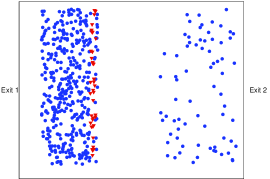
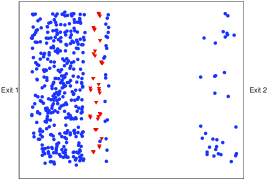
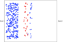
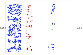
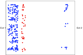
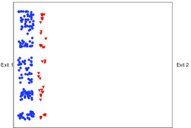
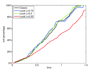
We illustrate the dynamics of the microscopic model in a two-dimensional symmetric corridor $\Omega=[0,1]\times[0,\frac{1}{2}]$ with exits at the left and right side, i.e. $x=0$ and $x=1$. The 1D case of section 5.1 can be interpreted as a projection of this two-dimensional geometry. We consider the same initial distribution of individuals, i.e. the positions of all $500$ particles are distributed according to the initial pedestrian density (19). For $L=0.25$, Figure 6(a)-(f) nicely illustrates a similar turn-around behavior as in the 1D macroscopic simulations. At the beginning the group close to the left exit splits, one part exits through the left exit the other one moves towards the more distant right exit. As the density close to the left exit decreases in time, the group moving towards the more distant exit splits again, i.e. parts of the group turn around and move back again. We marked all individuals, which initially moved towards the right but then turn around, with red triangles. Furthermore, Figure 6(g) shows the change of the evacuation performance for different sizes of the local vision cones $L$. Here we plot the percentage of the total initial mass outside the domain versus time. Decreasing $L$ and hence the perceived information, we observe that the overall evacuation performance first is merely diminished, and only begins to drop significantly after a certain threshold. The evacuation time will approach the uninformed eikonal case $L=0$, which is not shown. All parameters can be found in Appendix A.2.

5.3. 2D non-symmetric corridor - macroscopic model

Now we turn to the macroscopic model in two dimensions. Again we consider the corridor $\Omega=[0,1]\times[0,\frac{1}{2}]$, the exits however form only a part of the left and right edges, hence we obtain a fully two-dimensional dynamics where boundary conditions matter. The left exit is located between $(0,0)$ and $(0,0.1)$ and the right exit is the segment connecting $(1,\tfrac{1}{2})$ and $(1,0.4)$. The initial density Figure 7(a) is given as a low density group of pedestrians on the left and a high density group on the right

(20) $$\rho_{0}(x,y)=\begin{cases}0.1&0.05\leq x\leq 0.3\,,\,0\leq y\leq 0.25,\\ 0.95&0.6\leq x\leq 0.95,\\ 0&\text{otherwise}.\end{cases}$$
Refer to caption
(a) Time $t=0$
Refer to caption
(b) Time $t=0.8$
Refer to caption
(c) Time $t=1.07$
Refer to caption
(d) Time $t=1.4$
Refer to caption
(e) Time $t=2.1$
Refer to caption
(f) Time $t=2.75$
Figure 7. Two-dimensional macroscopic dynamics : We simulate model (11) with global visual perception $V_{x}=\Omega$. Two groups of pedestrians are initially placed in a corridor with a lower left and an upper right exit. The high density group separates according to the path optimization mechanism, as illustrated in several time snapshots of the density in (a) - (f). The right exit is vacated before the left exit and the final evacuation time (not shown here) is $\approx 3.4$.

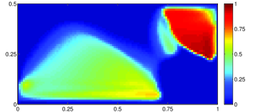
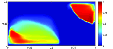
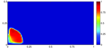
We first study the case of global vision $L=\infty\Leftrightarrow V_{x}=\Omega$ in Figure 7. In (b), the low density group turns towards left and is quickly vacated. The high density group on the other side splits along a curve of sonic points. Pedestrians turning to the right cause a jam in front of the right exit, whereas left-turning pedestrians occupy the corridor in a rarefaction-type manner inherited by the physical flux law (18). Upon arrival at the left exit, pedestrians pile up and form a new jam (c). Hence, a fraction of the density turns around again and heads for the right exit (d, around $(0.5,.25$)), having to cross most of the corridor again (e). However, most of the pedestrians are committed to the left exit and do not turn, because the severeness of the left jam does not compensate their expected travel time, and the left exit is vacated later than the right exit (f).

Compared to the classical Hughes model, the relaxation term (9) and the conviction-based interaction (11b)-(11c) allow for a smooth turning behaviour. The wall-repulsion (10) causes a density gap, which is different to zero-flux conditions as in [26], but prevents any spurious effects of the boundary flux.

Refer to caption
(a) Time $t=0.25$
Refer to caption
(b) Time $t=0.8$
Refer to caption
(c) Time $t=1.07$
Refer to caption
(d) Time $t=1.4$
Refer to caption
(e) Time $t=2.1$
Refer to caption
(f) Time $t=2.75$
Figure 8. Two-dimensional macroscopic dynamics : We simulate model (11) with local visual perception $L=0.75$ and the same initial configuration as Figure 7. In the time snapshots of the density, we observe again an initial separation of the high density group (a). A waiting phenomena of up to two local groups is clearly observed (b-d). Crucially, waiting pedestrians are able to choose their exit later (d-e), which leads to a rather simultaneously clearing of both jams (f), as opposed to Figure 7. The final evacuation time (not shown here) is $\approx 3.025$.

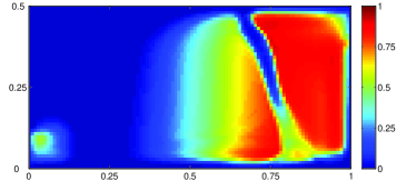
It is clear that even the planning algorithm incorporated into the classic Hughes’ model does not lead to an optimal evacuation. One reason for suboptimality in Figure 7 is that pedestrians have to keep in motion constantly but cannot predict the occurrence of future jams. Hence, pedestrians are likely to walk towards an exit that will be blocked in the future, as seen in the example.

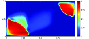
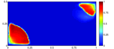
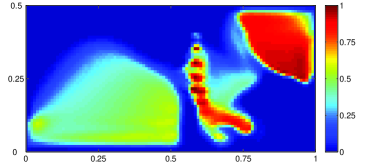
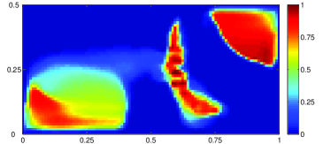
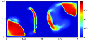
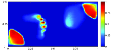
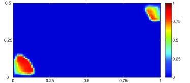
In Figure 8 we study the same initial configurations with localised perception and a radial vision cone of diameter $L=0.75$. The initial separation phase (a) is similar to Figure 7. As pedestrians move from the right to the left, the right jam gets out of sight and its influence diminishes. At the same time, the density on the left becomes visible. At a certain point a balance is achieved and pedestrians locally accumulate around an area of equal walking costs, where in this case they are able to stop (b-c). Hence, we observe a waiting behavior which cannot be observed in classical Hughes’ type models. Looking from (c) to (d), a high density jam forms at the left exit, which causes part of the left-walking pedestrians to turn right after enough conviction is gathered. Together with some outflow of the first waiting group, a second waiting group is formed (d). Pedestrians in a waiting group choose to move if one direction becomes favorable. As both jams at the exits reduce at the same rate, the left waiting group walks to the left and vice versa (e). Finally, the waiting groups dissolve and the exits get vacated at a rather similar time (f), and the evacuation time improves compared to Figure 7.

Refer to caption
Figure 9. Evacuation time of the macroscopic model for varying vision cone diameters $L$: The performance can improve with limited vision. $L=0$ corresponds to the eikonal case whereas $L>2.5$ implies unlimited vision in the given corridor.

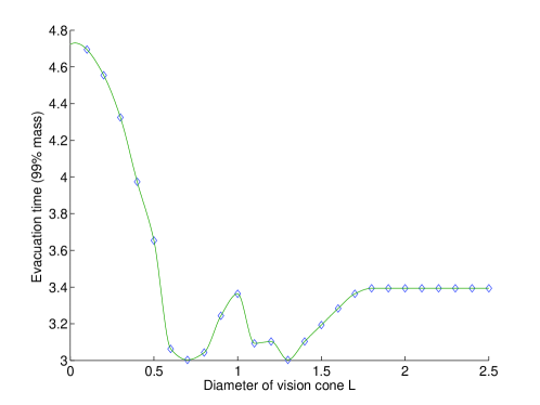
The fact that evacuation performance can improve under limited perception of information is surprising at first glance. Our simulations give an good explanation for the phenomena: As pedestrians show a waiting behaviour, they are less likely to be trapped in the jam arising at the left exit. In fact, the waiting is made possible by the combined effect of multiple sonic points due to local vision and the smoothed turning mechanism. Naturally, this is not generally the case and cannot be a-priori answered. For small vision lengths $L$, the dynamics will converge to the velocity field given by the eikonal equation, which is our initial configuration will exit almost all pedestrians using the right exit and perform poorly. In Figure 9, we study the evacuation time of $99\%$ of the initial mass as a function of the diameter $L$. We unexpectedly find in this case wo optimal values of $L$ for which the evacuation time is minimal. The classical Hughes’ evacuation time ($L$ large) is always less or equal than the eikonal case ($L=0$), however there is no way to generally argue that there will always be a minimum in between.

6. Conclusion

In this work we introduced a localized smooth variant of Hughes’s model for pedestrian crowd dynamics. We regularised the original model, composed by an eikonal equation and a continuity equation. First by a local interaction term, which intermediates individual pointwise path optimisation towards conviction-weighted walking directions. Secondly, we allowed pedestrians to stop, if they are undecided, using a smooth approximation of the normalization condition. Most importantly, we restrict the information on the global density each pedestrian can use for her planning algorithm to a local surrounding area. This is a very realistic assumption for large crowds that has not been considered in the literature so far. We presented both a microscopic and a macroscopic version, and illustrated the model components in the one-dimensional case. In terms of analytical results, a rigorous theory for these kind of equations in multiple dimensions is currently out of reach to the best of our knowledge. However, we were able to identify some qualitative properties of the dependence of the optimal path on the vision cone that allow for a reduction of complexity.

The numerical approximation of the model on both levels has been discussed and utilizes several techniques including sweeping and marching methods, particle approximations and finite volume schemes. Though the numerical costs of computing a solution have increased due to the inhomogeneity of vision cones, we observe new effects and phenomena in the model based on our simulations. First, local groups of pedestrians are able to change repeatedly their walking direction towards an exit. This ’multiple turn-around behaviour’ can explained by the multiple sonic points of the estimated walking costs, which by construction cannot occur in the classical case. We stress that the smoothening and conviction terms are crucial to allow a swift turning behavior, which is not trivial to model in first order equations. Second, the model replicates a waiting behaviour in case of undecided pedestrians, i.e. in areas where locally estimated walking costs towards different exits are equal. Surprisingly, we found that this waiting phenomena induced by localized information can improve the overall evacuation performance of the crowd. In our numerical example we observed two local minima when varying the vision cone diameter.

To conclude, we have demonstrated that local vision effects can be implemented into first order models for crowd dynamics. This leads to new unforeseen phenomena and complex behavior, whose partial understanding via qualitative properties is important for the applicability of such equations to social-economic problems. On the other hand, this work illustrates the limitations to first order models such as Hughes’, where planning decisions are instantaneously updated and no social or cognitive memory is taken into account. From our point of view Hughes’ type equations constitute an important building block for crowd models and a mathematically important object of study, but it cannot be expected to be fully realistic.

Acknowledgment

JAC acknowledges support from projects MTM2011-27739-C04-02 and the Royal Society through a Wolfson Research Merit Award. JAC and SM were supported by Engineering and Physical Sciences Research Council (UK) grant number EP/K008404/1. MTW acknowledges financial support from the Austrian Academy of Sciences ÖAW via the New Frontiers Group NSP-001. Preprint of an article submitted for consideration in Mathematical Models and Methods in Applied Sciences, ©2015 World Scientific Publishing Company, http://www.worldscientific.com/worldscinet/m3as.

Appendix A Simulation parameters

A.1. 1d macro parameters in Section 5.1

The macroscopic simulation in 1D was implemented in MATLAB. The domain $[0,1]$ was uniformly discretized with $\Delta x=10^{-4}$. The time step was set to $\Delta t=5\cdot 10^{-5}.$ The vision cone was defined as $V_{x}=[x-L/2,x+L/2]\cap[0,1]$ with $L=0.75$. The radial interaction kernel $\mathcal{K}$ was chosen as the indicator function on the interval $[0,0.05]$. The smoothed projection operator was chosen as in (9) with $\ell=0.05$ and $k=25$. The wall repulsion $W(x)$ was neglected in 1D. Absorbing boundary conditions were applied at both exits. The cost function was numerically bounded at $c(\rho)\leq 10^{4}$.

A.2. 2d micro parameters in Section 5.2

The microscopic simulations are implemented using the software package Netgen/NgSolve. The domain was discretized in $1438$ triangles, the time steps were set to $\Delta t=10^{-2}$, the final time to $T=1.5$. At time $t=0$ we distributed the $500$ particles according to the initial datum $\rho_{0}$ used in subsection 5.1. The empirical density $\rho^{N}_{g}$ was calculated using Gaussians with variance $\sigma=0.05$ for the smooth approximation $g$. The width of the local vision cone was set to $L=0.25$ in Figure 6(a)-(e) and to $L=0.75,0.5$ and $L=0.25$ in Figure 6(f).

A.3. 2d macro parameters in Section 5.3

The macroscopic simulation in 2D was implemented in MATLAB. The domain $\Omega=[0,1]\times[0,\frac{1}{2}]$ was uniformly discretized with $\Delta x=\Delta y=10^{-3}$. The time step was set to $\Delta t=5\cdot 10^{-3}.$ A Fast Sweeping Method was used to solve the eikonal equations. The vision cone was defined as $V_{x}=\{y:\|y-x\|_{2}\leq\frac{L}{2}\}\cap\Omega$ with varying diameter $L$. The radial interaction kernel $\mathcal{K}$ was chosen as

$$\mathcal{K}(x)=\begin{cases}\exp\left(-\frac{b^{2}}{b^{2}-\|x\|^{2}}\right)&\|x\|\leq b,\\ 0&\text{else}.\end{cases}$$

with $b=0.05$. The smoothed projection operator was chosen as in (9) with $\ell=0.05$ and $k=25$. The wall repulsion $W(x)$ was defined with the width of the boundary layer function $\chi_{w}$ set to $w=0.025$. The wall costs $W(x)$ were numerically bounded at $W(x)\leq c(0.975)$. The cost function was numerically bounded at $c(\rho)\leq 10^{3}$. The numerical accuracy for vanishing density was set to $10^{-7}$.

References

  • [1] D. Amadori and M. Di Francesco. The one-dimensional Hughes’ model for pedestrian flow: Riemann–type solutions. Acta Mathematica Scientia, 32(1):259–280, 2012.
  • [2] P. Amorim, R. M. Colombo, and A. Teixeira. On the numerical integration of scalar nonlocal conservation laws. ESAIM: Mathematical Modelling and Numerical Analysis, eFirst, 12 2014.
  • [3] C. Appert-Rolland, P. Degond, and S. Motsch. Two-way multi-lane traffic model for pedestrians in corridors. Netw. Heterog. Media, 6(3):351–381, 2011.
  • [4] M. Bardi and I. Capuzzo-Dolcetta. Optimal control and viscosity solutions of Hamilton-Jacobi-Bellman equations. Systems & Control: Foundations & Applications. Birkhäuser Boston, Inc., Boston, MA, 1997.
  • [5] N. Bellomo, A. Bellouquid, and D. Knopoff. From the microscale to collective crowd dynamics. Multiscale Modeling & Simulation, 11(3):943–963, 2013.
  • [6] N. Bellomo and C. Dogbe. On the modeling of traffic and crowds: A survey of models, speculations, and perspectives. SIAM Review, 53(3):409–463, 2011.
  • [7] N. Bellomo, B. Piccoli, and A. Tosin. Modeling crowd dynamics from a complex system viewpoint. Mathematical Models and Methods in Applied Sciences, 22(supp02):1230004, 2012.
  • [8] S. Blandin and P. Goatin. Well-posedness of a conservation law with non-local flux arising in traffic flow modeling. hal-00954527.
  • [9] M. Burger, M. Di Francesco, P. Markowich, and M.-T. Wolfram. Mean field games with nonlinear mobilities in pedestrian dynamics. DCDS B, 19(5):1311–1333, 2014.
  • [10] C. Burstedde, K. Klauck, A. Schadschneider, and J. Zittartz. Simulation of pedestrian dynamics using a two-dimensional cellular automaton. Physica A: Statistical Mechanics and its Applications, 295(3):507–525, 2001.
  • [11] R. M. Colombo, M. Garavello, and M. Lécureux-Mercier. A class of nonlocal models for pedestrian traffic. Mathematical Models and Methods in Applied Sciences, 22(04), 2012.
  • [12] R. M. Colombo and M. Lécureux-Mercier. Nonlocal crowd dynamics models for several populations. Acta Mathematica Scientia, 32(1):177–196, 2012.
  • [13] G. Crippa and M. Lécureux-Mercier. Existence and uniqueness of measure solutions for a system of continuity equations with non-local flow. Nonlinear Differential Equations and Applications NoDEA, 20(3):523–537, 2013.
  • [14] E. Cristiani, B. Piccoli, and A. Tosin. Multiscale modeling of granular flows with application to crowd dynamics. Multiscale Modeling & Simulation, 9(1):155–182, 2011.
  • [15] P. Degond, C. Appert-Rolland, M. Moussa d, J. Pettr , and G. Theraulaz. A hierarchy of heuristic-based models of crowd dynamics. Journal of Statistical Physics, 152(6):1033–1068, 2013.
  • [16] P. Degond, C. Appert-Rolland, J. Pettré, and G. Theraulaz. Vision-based macroscopic pedestrian models. Kinet. Relat. Models, 6(4):809–839, 2013.
  • [17] M. Di Francesco, P. A. Markowich, J.-F. Pietschmann, and M.-T. Wolfram. On the Hughes’ model for pedestrian flow: The one-dimensional case. Journal of Differential Equations, 250(3):1334–1362, 2011.
  • [18] C. Dogbé. Modeling crowd dynamics by the mean-field limit approach. Mathematical and Computer Modelling, 52(9):1506–1520, 2010.
  • [19] M. Dumbser, A. Hidalgo, M. Castro, C. Parés, and E. F. Toro. FORCE schemes on unstructured meshes II: Non-conservative hyperbolic systems. Computer Methods in Applied Mechanics and Engineering, 199(9-12):625–647, Jan. 2010.
  • [20] N. El-Khatib, P. Goatin, and M. D. Rosini. On entropy weak solutions of Hughes model for pedestrian motion. Zeitschrift für angewandte Mathematik und Physik, 64(2):223–251, 2013.
  • [21] P. Goatin and M. Mimault. The wave-front tracking algorithm for Hughes’ model of pedestrian motion. SIAM Journal on Scientific Computing, 35(3):B606–B622, 2013.
  • [22] D. Helbing, I. Farkas, and T. Vicsek. Simulating dynamical features of escape panic. Nature, 407(6803):487–490, 2000.
  • [23] D. Helbing and P. Molnar. Social force model for pedestrian dynamics. Physical review E, 51(5):4282, 1995.
  • [24] D. D. Holm. Geometric mechanics. Part I. Imperial College Press, London, second edition, 2011. Dynamics and symmetry.
  • [25] S. P. Hoogendoorn and P. Bovy. Pedestrian route-choice and activity scheduling theory and models. Transportation Research Part B: Methodological, 38(2):169–190, 2004.
  • [26] L. Huang, S. Wong, M. Zhang, C.-W. Shu, and W. H. Lam. Revisiting hughes dynamic continuum model for pedestrian flow and the development of an efficient solution algorithm. Transportation Research Part B: Methodological, 43(1):127 – 141, 2009.
  • [27] R. L. Hughes. A continuum theory for the flow of pedestrians. Transportation Research Part B: Methodological, 36(6):507–535, 2002.
  • [28] R. Kimmel and J. A. Sethian. Computing geodesic paths on manifolds. Proceedings of the National Academy of Sciences, 95(15):8431–8435, 1998.
  • [29] A. Lachapelle and M.-T. Wolfram. On a mean field game approach modeling congestion and aversion in pedestrian crowds. Transportation research part B: methodological, 45(10):1572–1589, 2011.
  • [30] M. J. Lighthill and G. B. Whitham. On kinematic waves. ii. a theory of traffic flow on long crowded roads. Proceedings of the Royal Society of London A: Mathematical, Physical and Engineering Sciences, 229(1178):317–345, 1955.
  • [31] M. Moussaid, E. G. Guillot, M. Moreau, J. Fehrenbach, O. Chabiron, S. Lemercier, J. Pettre, C. Appert-Rolland, P. Degond, and G. Theraulaz. Traffic instabilities in self-organized pedestrian crowds. PLoS computational biology, 8(3), 2012.
  • [32] J. Qian, Y. Zhang, and H. Zhao. Fast sweeping methods for eikonal equations on triangular meshes. SIAM Journal on Numerical Analysis, 45(1):83–107, 2007.
  • [33] P. I. Richards. Shock waves on the highway. Operations Research, 4(1):42–51, 1956.
  • [34] J. A. Sethian. Fast marching methods. SIAM Rev., 41(2):199–235, June 1999.
  • [35] E. F. Toro, A. Hidalgo, and M. Dumbser. Force schemes on unstructured meshes i: Conservative hyperbolic systems. Journal of Computational Physics, 228(9):3368–3389, 2009.
  • [36] A. Treuille, S. Cooper, and Z. Popović. Continuum crowds. ACM Trans. Graph., 25(3):1160–1168, July 2006.
  • [37] F. Venuti and L. Bruno. Crowd-structure interaction in lively footbridges under synchronous lateral excitation: A literature review. Physics of Life Reviews, 6(3):176 – 206, 2009.
  • [38] H. Zhao. A fast sweeping method for eikonal equations. Mathematics of Computation, 74:603–627, 2005.