Abstract: We consider normal forms in ‘magnetic bottle’ type Hamiltonians of the form $H=\frac{1}{2}(\rho^{2}_{\rho}+\omega^{2}_{1}\rho^{2})+\frac{1}{2}p^{2}_{z}+hot$ (second frequency $\omega_{2}$ equal to zero in the lowest order). Our main results are: i) a novel method to construct the normal form in cases of resonance, and ii) a study of the asymptotic behavior of both the non-resonant and the resonant series. We find that, if we truncate the normal form series at order $r$, the series remainder in both constructions decreases with increasing $r$ down to a minimum, and then it increases with $r$. The computed minimum remainder turns to be exponentially small in $\frac{1}{\Delta E}$, where $\Delta E$ is the mirror oscillation energy, while the optimal order scales as an inverse power of $\Delta E$. We estimate numerically the exponents associated with the optimal order and the remainder’s exponential asymptotic behavior. In the resonant case, our novel method allows to compute a ‘quasi-integral’ (i.e. truncated formal integral) valid both for each particular resonance as well as away from all resonances. We applied these results to a specific magnetic bottle Hamiltonian. The non resonant normal form yields theorerical invariant curves on a surface of section which fit well the empirical curves away from resonances. On the other hand the resonant normal form fits very well both the invariant curves inside the islands of a particular resonance as well as the non-resonant invariant curves. Finally, we discuss how normal forms allow to compute a critical threshold for the onset of global chaos in the magnetic bottle.

1 Introduction

‘Magnetic bottle’ type nonlinear Hamiltonian dynamical systems appear in various areas of physics and astronomy. Examples are plasma confinement machines, ion traps and charged particle measuring devices, planetary magnetospheres leading, e.g., to the formation of radiation belts, magnetic reconnection, magnetic bottles in the solar corona, etc. (see, for example, Dendy 1993, Gurnett and Bhattacharjee 2005, and references therein).

It is well known that in such configurations there exist both regular and chaotic particle orbits. The regular orbits are of oscillatory nature, i.e., a gyration around the magnetic field lines combined with a ‘mirror’ oscillation along the field lines. A bouncing of the particles appears when the magnetic field lines converge towards a preferential direction (see e.g. Jackson 1962). A magnetic bottle is formed when there are two distinct domains along the field lines in which we have such a convergence. The particles are reflected as they approach the two ‘necks’ of the bottle. The mirror frequency is of order $\omega_{z}=O(|V_{\perp}^{2}(\partial^{2}B_{\perp}/\partial\rho\partial z)/B_{z})^{1/2}|)$, where $V_{\perp}$ is the gyration velocity, $B_{z}$, $B_{\perp}$ are the measures of the magnetic field along and accross the preferential direction (denoted by $z$) respectively, and $\rho\perp z$. One typically has $\omega_{z}<<\omega_{c}$, where $\omega_{c}=B_{z}q/m$ is the gyrofrequency of a particle of charge $q$ and mass $m$.

A basic form of adiabatic theory (see, for example, Jackson 1962, or Lichtenberg and Lieberman 1992), describes mirror oscillations as a consequence of the preservation of a so-called ‘adiabatic invariant’. To lowest order, this corresponds to the particle’s magnetic dipole moment $\mu=qV_{\perp}^{2}/(2\omega_{c})$. The determination of higher order (in powers of $\mu$) adiabatic invariants is a classical problem of dynamics. Several methods to deal with this problem are discussed in Kruskal (1962), Northrop (1963), Contopoulos (1965), Dragt (1965), Arnold et al. (1988), Lichtenberg and Lieberman (1992) and Benettin et al. (1999).

For magnetic bottle Hamiltonians quite efficient methods can be derived in the context of canonical perturbation theory. Such methods have been proposed by Contopoulos and Vlahos (1975), and Dragt and Finn (1979). In the canonical context, one starts from the basic Hamiltonian

$$H={1\over 2m}\left(\mathbf{p}-q\mathbf{A}\right)^{2}$$ (1)

where $\mathbf{A}$ is the vector potential corresponding to the magnetic field $\mathbf{B}=\nabla\times\mathbf{A}$ and $\mathbf{p}$ are generalized momenta conjugate to the position variables. Assuming, in the simplest case, axisymmetry around the z-axis, the Hamiltonian in cylindrical co-ordinates $(\rho,z)$ takes the form

$$H={p_{\rho}^{2}\over 2}+{1\over 2}\omega_{1}^{2}\rho^{2}+{p_{z}^{2}\over 2}+...$$ (2)

with $\omega_{1}=\omega_{c}$ for particles gyrating around the z-axis. Note that the equations of motion arising from the quadratic terms in the Hamiltonian (2) represent a case of so-called ‘nilpotent’ linearization, since one of the eigenvalues of the matrix of the linearized system of equations is equal to zero. There is a variety of methods for constructing a normal form for such systems (see, for example, Meyer (1984), Cushman and Sanders (1986), Elphick (1988), Baider and Sanders (1991), as well as Sanders et al. (2007) for a review). On the other hand, the canonical approach leads to a definition of action-angle variables for the magnetic bottle, admitting straightforward physical interpretation. In particular, if we define the pair of action-angle variables $(J_{1},\phi_{1})$ via

$$\rho=\sqrt{2J_{1}\over\omega_{1}}\sin\phi_{1},~{}~{}~{}p_{\rho}=\sqrt{2\omega_{1}J_{1}}\cos\phi_{1}~{}~{},$$ (3)

the quantity $J_{1}$ is proportional to the magnetic dipole moment, i.e., $J_{1}=mV_{\perp}^{2}/(2\omega_{c})$ $=(m/q)\mu$. After some steps of perturbation theory, we can then define new canonical variables $(\theta_{1},I_{1},\zeta,P_{\zeta})$, which are near-identity transformations of the old canonical variables $(\phi_{1},J_{1},z,p_{z})$, so that the Hamiltonian in the new variables takes the form:

$$H(\theta_{1},I_{1},\zeta,P_{\zeta})=Z(I_{1},\zeta,P_{\zeta})+R(\theta_{1},I_{1},\zeta,P_{\zeta})~{}~{}.$$ (4)

The function $Z$, called normal form, has the form

$$Z(I_{1},\zeta,P_{\zeta})=\omega_{1}I_{1}+{1\over 2}(P_{\zeta}^{2}+\omega_{2}^{2}(I_{1})\zeta^{2})+...$$ (5)

The action $I_{1}$ would be an exact integral of the Hamiltonian flow under $Z$ alone. On the other hand, the function $R$, called ‘remainder’, depends on the angle $\theta_{1}$, thus it introduces some time variations of $I_{1}$ under the complete Hamiltonian flow of (5). Nevertheless, one typically has that $|R|<<|Z|$, implying that the effect of the remainder on dynamics is small. Hence, $I_{1}$ represents a quasi-integral of motion, i.e. a high-order adiabatic invariant, while the mirror frequency $\omega_{2}$ (assumed small) is expressed by this theory as a function of $I_{1}$.

The convergence behavior of the magnetic bottle normal form series at high normalization orders has not yet been fully explored. A systematic study of the convergence is presented in Engel et al. (1995). These authors considered a polynomial magnetic bottle model. Then, they computed a polynomial form of a ‘quasi-integral’ up to degree 14 in the canonical variables. From the numerical data, they distinguish three types of behavior, i.e., i) convergence, ii) non-convergence, and (iii) ‘pseudo-convergence’, depending on the behavior of the numerical variations of their quasi-integral at various normalization orders up to order 14. Here, we extend this analysis to much higher orders, and provide a numerical estimate of the asymptotic behavior of the series based on the size of the remainder of the normal form. In agreement with basic theory, we observe numerically that the only existing behavior is ‘pseudo-convergence’, i.e., the series exhibit always an asymptotic behavior. This means that an ‘optimal’ normalization order $r_{opt}$ can be identified, up to which the remainder decreases in size, yielding the impression that the normalization is convergent, while, beyond the optimal order, the size of the remainder increases with the normalization order, thus the normalization turns always to be divergent. We also provide evidence that the crucial small quantity which enters in all asymptotic estimates is the energy $\Delta E$ of the mirror oscillations. Asymptotically, one has the estimates $r_{opt}={\cal O}(\Delta E^{-\alpha})$, for the optimal order, and $||R||_{opt}={\cal O}(\exp(-1/\Delta E^{\gamma}))$ for the size of the remainder at the optimal order, with exponents $\alpha$ and $\gamma$ specified numerically in section 3 below. We note that theoretical exponential estimates on adiabatic invariants in nonlinear modulated oscillators are discussed in Neishtadt (1981,1984) and Benettin and Sempio (1994) (for the case of linear oscillators, see Howard (1970) and references therein).

The second main result in the present paper regards the construction of a normal form in magnetic bottle Hamiltonians in a case not covered by the usual theory, namely the case of resonances. Resonances appear whenever the condition $\omega_{2}/\omega_{1}=m_{2}/m_{1}$ is satisfied for non-zero integers $m_{1},m_{2}$. Such values are marked by the bifurcation of new periodic orbits (in pairs stable-unstable) from a so-called ‘central’ (equatorial) periodic orbit ($z=0$). The most important resonances are of the form $\omega_{1}-n\omega_{2}=0$, with $n$ integer. Resonances of lower and lower order appear by increasing the energy. The appearance of the lowest resonances 1:4, 1:3, 1:2, marks an overall qualitative change of the phase space structure leading eventually to the onset of global chaos.

The usual (non-resonant) normal form can predict the values of $I_{1}$ when new resonances bifurcate, as well as the distance of the resonances from the central orbit as $I_{1}$ increases (Contopoulos and Vlahos 1975). Nevertheless, it cannot describe the structure of the phase space near resonances. Here, precisely, we propose a method of construction of a resonant normal form for magnetic bottle Hamiltonians, which is applicable both for resonant orbits of one (at a time) specific resonance as well as for the non-resonant orbits in its neighborhood. Our method can be viewed as a combination of two recently introduced techniques: these are i) ‘detuning’ (see Pucacco et al. 2008), and ii) ‘book-keeping’ (see Efthymiopoulos 2008, 2012). Both techniques reflect ways to optimize the formal treatment of various small quantities appearing in the formal series. The main difference between the usual non-resonant construction and the hereby proposed resonant construction is the following: In the case of non-resonant series, we select as small parameter either the frequency $\omega_{2}$ or the distance (in phase space) from the central orbit (see Contopoulos (1965) for a detailed comparison of the two approaches). In the resonant series, however, we simultaneously treat the distance from the central orbit and the small frequencies as small parameters. We note, finally, that the case presently dealt with is quite distinct from the case of resonance in models with a periodic space modulation of the magnetic field (as e.g. in Dunnett et al. 1968, McNamara 1978).

Implementing our algorithm we compute high order resonant quasi-integrals, and check their degree of accuracy in comparison with the invariant curves found numerically on the domain of regular motion, using as reference the same model as Engel et al. (1995). In the same way as for the non-resonant normal form, we also here examine the asymptotic behavior of the resonant formal series. We demonstrate that in this case as well there hold exponential estimates for the dependence of the optimal normalization order, as well as the size of the optimal remainder, on the mirror oscillation energy $\Delta E$. As a final outcome, we use the magnetic bottle normal forms in order to analytically compute the critical energy beyond which the central periodic orbit becomes unstable. This determines the energy where we have the onset of global chaos in the magnetic bottle.

The paper is organized as follows. Section 2 briefly describes some features of the reference model (Engel et al. 1995) used in our study, for the paper’s self-containedness. Section 3 describes the algorithm of computation of the non-resonant normal form. We emphasize that this is not a new method but essentially the same as in Dragt and Finn (1979) and Engel et al (1995). Also, here as well we employ the method of Lie series which is quite convenient for performing near-identity canonical transformations (Hori (1966), Deprit (1969)). However, we present the specific algorithmic steps in greater detail than in these earlier papers, in order to set the context and introduce the notation of the ‘book-keeping’ technique (Efthymiopoulos 2012). The main new result in this section regards the numerical study of the asymptotic properties of the non-resonant series and the determination of the associated exponents entering in exponential estimates of the size of the optimal remainder. These are found by extending all normal form computations up to a high order. Section 4 describes the novel computation of the resonant normal form construction for magnetic bottle Hamiltonians. Here, also, we study numerically the normal form’s asymptotic behavior by reaching sufficiently high normalization orders. Finally, we compute approximately the threshold for the onset of global chaos using normal forms. Section 5 summarizes our conclusions.

2 Hamiltonian model

We consider the same axisymmetric magnetic bottle model as in Engel et al. (1995). The magnetic field is given by $\mathbf{B}=\mathbf{\nabla}\times\mathbf{A}$, where $\mathbf{A}$ is the vector potential given in cylindrical coordinates by $\mathbf{A}\equiv$ $(A_{\rho},A_{\phi},A_{z})=$ $(0,A_{\phi},0)$ with

$$A_{\phi}={B_{0}\over 2}\left(\rho-\beta_{1}({1\over 8}\rho^{3}-{1\over 2}\rho z^{2})\right)~{}~{}.$$ (6)

$B_{0}$ is the value of the homogeneous (along $z$) magnetic field component and $\beta_{1}$ measures the strength of the (octupole) component causing the mirroring effect. In the physical context, $\beta_{1}$ represents a small parameter. The equations of motion for a particle of mass $m=1$ and charge $q=1$ are derived from the Hamiltonian

$$H={1\over 2}\left(\mathbf{p}-\mathbf{A}\right)^{2}={p_{z}^{2}\over 2}+{p_{\rho}^{2}\over 2}+{p_{\phi}^{2}\over 2\rho^{2}}-{A_{\phi}p_{\phi}\over\rho}+{A_{\phi}^{2}\over 2}~{}~{}.$$ (7)

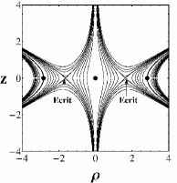
Figure 1: The family of equipotential curves or curves of zero velocity (CZV), $E$=$V(\rho,z)=A_{\phi}^{2}/2$, for various values of $E$. $E_{crit}$=$0.\overline{592}$ is the value of $V(r,0)$ at its local maximum, and the dots indicate the local minima $E=0$.

Since $\phi$ is ignorable in (7), $p_{\phi}$ is an integral of motion. The system can be considered as of two degrees of freedom, with ‘effective potential’:

$$V_{eff}={p_{\phi}^{2}\over 2\rho^{2}}-{A_{\phi}(\rho,z)p_{\phi}\over\rho}+{A_{\phi}^{2}(\rho,z)\over 2}~{}~{}.$$ (8)

Orbits starting with $z=0$, $p_{z}=\dot{z}=0$ remain always on the equatorial plane $z=0$. For such orbits, the equations $\dot{\rho}=p_{\rho}=0$ and $\dot{p_{\rho}}=-\partial V_{eff}(\rho,z=0)/\partial\rho=0$ define two types of equilibria for any fixed radius $\rho$:

i) For $p_{\phi}<0$ the equilibrium solution is $\rho=\rho_{c}=[-p_{\phi}\/\partial A_{\phi}/\partial\rho)_{\rho=\rho_{c},z=0}]^{1/2}$. This yields a circular equatorial orbit surrounding the central axis, with gyration frequency $\omega_{c}={p_{\phi}/\rho_{c}^{2}}-A_{\phi}(\rho_{c},0)/\rho_{c}<0$. Nearby orbits can be studied by means of the epicyclic approximation. Setting $\xi=\rho-\rho_{c}$ and expanding the Hamiltonian around the circular solution we arrive at:

$$H=\mbox{const}+{p_{z}^{2}\over 2}+{p_{\xi}^{2}\over 2}+{1\over 2}\kappa^{2}\xi^{2}+H_{1}$$ (9)

where $\kappa^{2}=3p_{\phi}^{2}/\rho_{c}^{4}+2p_{\phi}A^{\prime}_{\phi}/\rho_{c}^{2}-2p_{\phi}A_{\phi}/\rho_{c}^{3}-p_{\phi}A^{\prime\prime}_{\phi}/\rho+A^{\prime\prime}_{\phi}A_{\phi}+(A^{\prime}_{\phi})^{2}$ (derivatives are with respect to $\rho$, evaluated at $\rho=\rho_{c},z=0$). It is easy to check that in $H_{1}$ the lowest order terms quadratic in $z$ are either of order $O(\beta_{1}z^{2})$ or $O(\xi z^{2})$, hence small. Thus, the Hamiltonian (9) is of the general form (2).

ii) For $p_{\phi}\geq 0$ one finds, instead, the equilibrium solution $\rho=\rho_{c}=p_{\phi}/A_{\phi}(\rho_{c},0)$ which yields $\dot{\phi}=0$. This solution describes a particle at rest at the distance $\rho_{c}$ for any value of the azimouth. Nearby orbits on the equatorial plane, keeping $p_{\phi}$ constant, arise by perturbing the radial velocity $\dot{\rho}\neq 0$ while keeping $\dot{\phi}=\dot{z}=0$. In this case, a similar analysis as above shows that nearby orbits describe gyrations around the equilibrium solution, which do not encircle the central axis. The gyration frequency is now equal to $\omega_{c}=\kappa$, the minimum and maximum distances from the axis are found by the two roots $0<\rho_{1}<\rho_{2}$ of $H=E=V_{eff}(\rho,0)$, while $\dot{\phi}$ has opposite sign in the intervals $\rho_{1}\leq\rho<\rho_{c}$ and $\rho_{c}<\rho\leq\rho_{2}$. The Hamiltonian is still given by (9), and it is easy to check that the lowest order terms quadratic in $z$ are of order $O(\xi z^{2})$. Thus, the Hamiltonian is again of the general form (2).

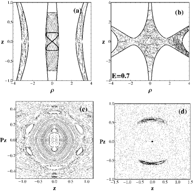
Figure 2: (a) The main types of orbits for $E=0.2$. The central orbit in gray is a typical non-resonant regular orbit undergoing mirror oscillations. The ‘figure 8’ orbit (black) is a 2:1 resonant orbit. Both orbits are limited by the central curves of zero velocity. On the other hand, the left and right gray curves show chaotic orbits limited by the outer CZVs. (b) A chaotic orbit for $E=0.7$, exploring the interior domain limited by the corresponding CZVs. (c) The surface of section $(z,p_{z})$ for $\rho=0$, $p_{\rho}>0$ at the energy $E=0.2$. Non-resonant regular orbits belong to invariant curves surrounding the central (equatorial) periodic orbit at $z=p_{z}=0$, while resonant orbits belong to island chains around the origin. The domain of stability is surrounded by a sea of chaotic orbits. (d) The surface of section at $E=0.7$, where global chaos prevails.

The simplest, albeit without loss of generality, case to consider is $p_{\phi}=0$, which we hereafter focus on. In this case, the orbital motion takes place on a meridian plane $(\rho,z)$ rotating with angular velocity $\dot{\phi}=-A_{\phi}/\rho$. Gyrating orbits cross the axis $\rho=0$. In order to formally avoid discontinuous transitions in the value of $\phi$ at each crossing, the cylindrical radius $\rho$ can be adopted to take both positive and negative values. In units in which $B_{0}=2$, $\beta_{1}=1$ in Eq.(6), the motion on the meridian plane is described by the Hamiltonian:

$$H(\rho,z,p_{\rho},p_{z})=\frac{1}{2}(p^{2}_{\rho}+p^{2}_{z})+V(\rho,z)$$ (10)

with a ‘potential’ (equal to $A_{\phi}^{2}/2$) given by

$$V(\rho,z)=\frac{1}{2}\rho^{2}+\frac{1}{2}\rho^{2}z^{2}-\frac{1}{8}\rho^{4}+\frac{1}{8}\rho^{2}z^{4}-\frac{1}{16}\rho^{4}z^{2}+\frac{1}{128}\rho^{6}~{}~{}.$$ (11)

Figure 1 plots the equipotential curves, or curves of zero velocity (CZV), for different values of the energy $E=H(\rho,z)=$ $V(\rho,z)$ with $p_{\rho}$ = $p_{z}$ = 0 (the magnetic field lines have a similar form (see figure 1 in Engel et al. (1995)), but form a small angle with the lines of Fig.1, which correspond to constant values of $A_{\phi}^{2}$ ). These curves define the limits that can be reached by the orbits. The potential along the $\rho$-axis ($z$=0) is $V(\rho,0)=\frac{1}{2}\rho^{2}(1-\frac{\rho^{2}}{8})^{2}=E$ and has two minima and one maximum (in each of the half-planes $\rho>0$ or $\rho<0$). The maximum is equal to $V(\rho,0)$=$E_{crit}$=16/27$\approx 0.5926$ for $\rho$= $\rho_{crit}$=$\pm\sqrt{8/3}\approx 1.633$.

Examples of orbits in the above system are given in Fig.2. When $0<E<E_{crit}$ there are three permissible regions of orbits, one close to the z-axis ($\rho=0$) and two on the right and on the left (Fig.2a). In the central region we find ordered orbits, which obey some quasi-integral of motion. The gray and black central orbits in Fig.2a correspond to a non-resonant and resonant case respectively. The associated phase portrait (surface of section $\rho=0$, $\dot{\rho}>0$) is shown in Fig2c, for the energy $E=0.2$. In this case, the main resonances are 2:1 and 3:1, which both produce double chains of islands of stability (four and six respectively in Fig.2c), as discussed in detail in section 4. On the other hand, in Fig.2a the left and right orbits in gray are chaotic orbits having no intersection with the surface of section of Fig.2c. Finally, for much higher energies ($E=0.7$, Figs2b,d), the central orbit has become unstable and the system is characterized by global chaos.

In section 4, we shall employ the normal form method in order to compute the critical energy value where the onset of global chaos takes place.

3 Non-resonant normal form

3.1 Algorithm

The Hamiltonian (10) is of the general form (1). A non-resonant normal form for this Hamiltonian can be constructed by the method of Dragt and Finn (1979) or Engel et al. (1995). We summarize here the main steps, introducing our own notation and terminology:

i) Introduction of complex canonical variables. Introducing the linear canonical change of variables

$$\rho={q_{1}+ip_{1}\over\sqrt{2\omega_{1,0}}},~{}~{}~{}p_{\rho}={iq_{1}+p_{1}\over\sqrt{2/\omega_{1,0}}},\\ z=q_{2},~{}~{}~{}p_{z}=p_{2}$$ (12)

with $\omega_{1,0}$ equal to the frequency induced by the quadratic term $O(\rho^{2})$ of the potential ($\omega_{1,0}=1$ in our example), the Hamiltonian takes the form $H=H_{2}+H_{4}+H_{6}$, with

$$H_{2}(q_{1},p_{1},p_{2})=i\omega_{1,0}q_{1}p_{1}+\frac{1}{2}p^{2}_{2}~{}~{}.$$ (13)

The terms $H_{4}$ and $H_{6}$ are of fourth and sixth degree respectively. For orbits crossing the z-axis (with $p_{\phi}=0$), $\omega_{1,0}$ is equal to half the gyration frequency.

ii) Book-keeping: We organize the terms in the Hamiltonian in groups of ‘different order of smallness’. Formally, we introduce a ‘book-keeping’ parameter $\lambda$, with numerical value $\lambda=1$, and write the Hamiltonian as

$$H\equiv H^{(0)}=H_{0}^{(0)}+\lambda H_{1}^{(0)}+\lambda^{2}H_{2}^{(0)}+...$$ (14)

The superscript $(0)$ means ‘no normalization step performed so far’. A subscript $i$, accompanied by a book-keeping coefficient $\lambda^{i}$, means “i-th order of smallness”. The arrangement of all the Hamiltonian terms in the groups $H^{(0)}_{0}$, $H^{(0)}_{1}$, etc., is done by adopting a ‘book-keeping rule’. For polynomial Hamiltonian models, the simplest choice of rule is to associate book-keeping order with polynomial degree. Thus, in the Hamiltonian (14) we set $H^{(0)}_{s}$ to be the ensemble of terms of polynomial degree $2s+2$. This renders our non-resonant construction equivalent to those of Dragt and Finn (1979) or Engel (1995). However, the above book-keeping rule will be modified in the resonant construction dealt with in section 4 below. We note here that the form of the Hamiltonian (section 2) in the more general case $p_{\phi}>0$ allows for employing the same book-keeping rule as above, with $\rho$ substituted by the local variable $\xi=\rho-\rho_{c}$ around an equatorial orbit at $\rho=\rho_{c}$. Instead, in the case $p_{\phi}<0$ we have to add one more power of $\lambda$ for every power of the quantity $\beta_{1}$, which now plays also the role of small parameter.

iii) Choice of ‘kernel set’ ${\cal M}$. To choose a ‘kernel set’ means to answer the question of which terms are kept in the normal form along the normalization process. In the present example, in the Hamiltonian there appear monomial terms of the form $q_{1}^{k_{1}}p_{1}^{l_{1}}q_{2}^{k_{2}}p_{2}^{l_{2}}$, where $k_{1},~{}l_{1},~{}k_{2},~{}l_{2}\geq 0$. For determining a non-resonant formal integral, it suffices to keep in the normal form the terms satisfying $k_{1}=l_{1}$. Then, the normal form takes the form $Z\equiv Z(q_{1}p_{1},q_{2},p_{2})$, i.e. its dependence on $q_{1},p_{1}$ is only through the product $q_{1}p_{1}$. Then, the quantity $I_{1}=iq_{1}p_{1}$ is a formal integral, since $\{I_{1},Z\}=0$ (where $\{\cdot,\cdot\}$ denotes the Poisson bracket). However, it is practical to exclude some further terms from the normal form. Namely, we also exclude the terms with $k_{1}=l_{1}$ but $l_{2}\neq 0$, except if $k_{1}=l_{1}=0$ and $l_{2}=2$, $k_{2}=0$. This means to retain terms of the form $I_{1}^{n}q_{2}^{k_{2}}$, for exponents $n\neq 0$, as well as the ‘kinetic’ term $\frac{1}{2}p_{2}^{2}$. Since $I_{1}$ is a formal integral, after these definitions the normal form reduces to the form $Z=\omega_{1}I_{1}+p_{2}^{2}/2+U(I_{1},q_{2})$, i.e. $Z$ takes the form of an one-degree of freedom oscillator ($\omega_{1}I_{1}$) plus a ‘kinetic’ and a ‘potential’ term for the second degree of freedom (for which $I_{1}$ acts as a parameter in the ‘potential’ $U(I_{1},q_{2})$).

In summary, as kernel set ${\cal M}$ we choose:

$${\cal M}=\left\{k_{1}=l_{1}~{}\mbox{and}~{}\left(k_{2}=0,l_{2}=2~{}\mbox{if}~{}k_{1}+l_{1}=0,~{}\mbox{or}~{}l_{2}=0~{}\mbox{if}~{}k_{1}+l_{1}>0\right)\right\}~{}~{}.$$ (15)

iv) Normalization. We construct the non-resonant normal form by using canonical transformations via Lie series (see, e.g., Efthymiopoulos 2012 for a tutorial introduction to Lie series). We thus introduce the sequence of transformations: $(q_{1},q_{2},p_{1},p_{2})$ $\rightarrow$ $(q_{1}^{(1)},q_{2}^{(1)},p_{1}^{(1)},p_{2}^{(1)})$, $\rightarrow$ $(q_{1}^{(2)},q_{2}^{(2)},p_{1}^{(2)},p_{2}^{(2)})$, $\rightarrow$, $\ldots$, where superscripts $(1)$, $(2)$,…,denote the new canonical variables after the first, second, etc., normalization steps. In the $r$-th step, the transformation is given in terms of a Lie generating function $\chi_{r}(q_{1}^{(r)},q_{2}^{(r)},p_{1}^{(r)},p_{2}^{(r)})$. The transformation of any function $f(q_{1}^{(r-1)},q_{2}^{(r-1)},p_{1}^{(r-1)},p_{2}^{(r-1)})$ in the new variables is found by replacing $(q_{1}^{(r-1)},q_{2}^{(r-1)},p_{1}^{(r-1)},p_{2}^{(r-1)})$ with $(q_{1}^{(r)},q_{2}^{(r)},p_{1}^{(r)},p_{2}^{(r)})$ in the arguments of $f$ and, then, by computing $f^{\prime}=\exp(L_{\chi_{r}})f$, where

$$\exp(L_{\chi_{r}})=\sum_{k=0}^{\infty}{1\over k!}L^{k}_{\chi_{r}}~{}~{},$$ (16)

$L_{\chi_{r}}=\{\cdot,\chi_{r}\}$ denoting the Poisson bracket operator. In particular, the variables themselves are transformed according to $q_{1}^{(r)}=\exp(L_{\chi_{r}})q_{1}^{(r-1)}(q^{(r)})$, where $q_{1}^{(r-1)}(q^{(r)})$ is the identity function (and similarly for the remaining variables). In the sequel, for simplicity we drop superscripts in the notation of the canonical variables.

The generating functions $\chi_{r}$, $r=1,2,\ldots$ are computed recursively. Namely, the Hamiltonian after $r-1$ normalization steps has the form

$$H^{(r-1)}=Z_{0}+\lambda Z_{1}+\lambda^{2}Z_{2}+\ldots+\lambda^{r-1}Z_{r-1}+\lambda^{r}H^{(r-1)}_{r}+\lambda^{r+1}H^{(r-1)}_{r+1}+\ldots$$ (17)

where all the terms in $Z_{0}$, $Z_{1}$,…,$Z_{r-1}$ are in normal form, i.e., they belong to ${\cal M}$. According to the book-keeping rule choosen in (ii), the terms $Z_{s}$, or $H^{(r-1)}_{s}$ are of polynomial degree $2s+2$. In particular, $Z_{0}\equiv H_{2}=i\omega_{1,0}q_{1}p_{1}+p_{2}^{2}/2$. Let $\tilde{H}^{(r-1)}_{r}$ denote the terms of $H^{(r-1)}_{r}$ not belonging to ${\cal M}$. The generating function $\chi_{r}$ is the solution to the homological equation

$$\{Z_{0},\chi_{r}\}=\left\{i\omega_{1,0}q_{1}p_{1}+{p_{2}^{2}\over 2},\chi_{r}\right\}=-\lambda^{r}\tilde{H}^{(r-1)}_{r}~{}~{}.$$ (18)

After computing $\chi_{r}$, we compute the transformed Hamiltonian

$$H^{(r)}=\exp(L_{\chi_{r}})H^{(r-1)}~{}~{}.$$ (19)

This is in normal form up to terms of book-keeping order $r$, namely

$$H^{(r)}=Z_{0}+\lambda Z_{1}+\lambda^{2}Z_{2}+\ldots+\lambda^{r}Z_{r}+\lambda^{r+1}H^{(r)}_{r+1}+\lambda^{r+2}H^{(r)}_{r+2}+\ldots$$ (20)

This completes one step of the normalization algorithm.

In order to solve the homological equation (18), we first decompose $\tilde{H}^{(r-1)}_{r}$ in the sum of monomials

$$\tilde{H}^{(r-1)}_{r}=\sum_{\begin{array}[]{c}{}^{k_{1},l_{1},k_{2},l_{2}>0}\\ {}^{k_{1}+l_{1}+k_{2}+l_{2}=2r+2}\end{array}}h_{k_{1},l_{1},k_{2},l_{2}}^{(r-1)}q_{1}^{k_{1}}p_{1}^{l_{1}}q_{2}^{k_{2}}p_{2}^{l_{2}}$$

with known coefficients $h_{k_{1},l_{1},k_{2},l_{2}}^{(r-1)}$. However, one notes that, contrary to the usual Birkhoff normal form around elliptic equilibria, in the present case, due to the presence of the term $p_{2}^{2}/2$ in $Z_{0}$, a monomial $q_{1}^{k_{1}}p_{1}^{l_{1}}q_{2}^{k_{2}}p_{2}^{l_{2}}$ does not constitute an eigenfunction of the linear operator $D_{Z_{0}}=\{Z_{0},\cdot\}$, since

$$D_{Z_{0}}q_{1}^{k_{1}}p_{1}^{l_{1}}q_{2}^{k_{2}}p_{2}^{l_{2}}=i(l_{1}-k_{1})\omega_{1,0}q_{1}^{k_{1}}p_{1}^{l_{1}}q_{2}^{k_{2}}p_{2}^{l_{2}}-k_{2}q_{1}^{k_{1}}p_{1}^{l_{1}}q_{2}^{k_{2}-1}p_{2}^{l_{2}+1}~{}~{}~{}.$$ (21)

Thus, the homological equation cannot be solved by term-by-term comparison of the coefficients as in the usual Birkhoff case. Instead, we form the sets of terms

$${\cal A}_{kl} = \Bigg{\{}a^{(r-1)}_{kl,n}q_{1}^{k}p_{1}^{l}q_{2}^{n}p_{2}^{2r+2-k-l-n}:k+l\leq 2r+2,$$

$$~{}~{}~{}~{}~{}~{}~{}~{}~{}~{}~{}~{}n=0,1,\ldots,2r+2-k-l\Bigg{\}}$$

where $a^{(r-1)}_{kl,n}\equiv-h^{(r-1)}_{k,l,n,2r+2-k-l-n}$ for given values of $k=k_{1}$ and $l=l_{1}$. Then, setting the generating function $\chi_{r}$ to contain a similar group of terms with (yet unknown) coefficients $b^{(r-1)}_{kl,n}$, the homological equation is decomposed in the set of linear systems of equations

$$\left(\begin{array}[]{ccccl}c_{kl}&1&{}\hfil&{}\hfil&{}\\ {}\hfil&c_{kl}&2&{}\hfil&{}\\ {}\hfil&{}\hfil&\ddots&\ddots&{}\\ {}\hfil&{}\hfil&{}\hfil&c_{kl}&2r+2-k-l\\ {}\hfil&{}\hfil&{}\hfil&{}\hfil&c_{kl}\\ \end{array}\right)\left(\begin{array}[]{c}b^{(r-1)}_{kl,0}\\ b^{(r-1)}_{kl,1}\\ \vdots\\ \vdots\\ b^{(r-1)}_{kl,2r+2-k-l}\\ \end{array}\right)=\left(\begin{array}[]{c}a^{(r-1)}_{kl,0}\\ a^{(r-1)}_{kl,1}\\ \vdots\\ \vdots\\ a^{(r-1)}_{kl,2r+2-k-l}\\ \end{array}\right)$$ (23)

where $c_{kl}=i(l-k)\omega_{1,0}$. If $l\neq k$, the system (23) can be solved by backward substitution, i.e. we first solve the last equation, then substitute and solve the previous one, etc. On the other hand, the choice of kernel set ${\cal M}$ implies that the normalization should eliminate from the normal form also terms with $k=l$ and $n=0,1,\ldots 2r+1-k-l$. Then we have $a^{(r-1)}_{kl,2r+2-k-l}=0$ and the last of Eqs.(23) becomes the identity $0=0$, while the remaining equations for $k=l$ form a diagonal system with non zero-determinant for the coefficients $b^{(r-1)}_{kl,n}$ with $n=1,2,\ldots 2r+2-k-l$ in terms of the coefficients $a^{(r-1)}_{kl,n}$ with $n=0,1,\ldots 2r+1-k-l$. Also, the coefficient $b^{(r-1)}_{kl,0}$ becomes arbitrary, and can be set equal to zero. This completely specifies the generating function $\chi_{r}$.

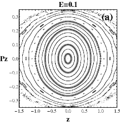
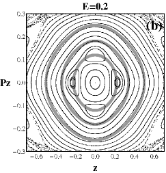
Figure 3: (a) The Poincaré surface of section for $E=0.1$ (black curves) superimposed with the curves of equal values of the non-resonant formal integral (gray points), truncated at order 5 (corresponding to polynomial degree 12). (b) Same as in (a) but for $E=0.2$. The non-resonant formal integral cannot reproduce the 2:1 islands of stability.

3.2 Implementation

Implementing the above procedure to the Hamiltonian (14), we compute a non-resonant normal form using a computer-algebraic program. At low normalization orders, this yields results similar to those of Engel et al. (1995). However, we extended the computations up to the normalization order $r=15$ (corresponding to the polynomial degree 32), while all series expressions were truncated at order $r_{trunc}=20$ (corresponding to polynomial degree 42). The asymptotic behavior of the series at high normalization orders is examined in the next subsection. At any rate, even at low normalization orders one obtains expressions for the non-resonant formal integral comparing well with numerical results for the non-resonant ordered orbits. As an example, after five normalization steps, the transformed Hamiltonian (restoring the book-keeping constant value $\lambda=1$) reads:

$$H^{(5)} = I_{1}-0.1875I_{1}^{2}-0.046875I_{1}^{3}-0.0256348I_{1}^{4}-0.0184021I_{1}^{5}-0.0152607I_{1}^{6}~{}~{}~{}~{}~{}~{}~{}~{}~{}~{}~{}~{}~{}$$

$$+ 0.5p_{2}^{2}+0.5I_{1}q_{2}^{2}+0.15625I_{1}^{2}q_{2}^{2}+0.1875I_{1}^{3}q_{2}^{2}+0.299194I_{1}^{4}q_{2}^{2}+0.551285I_{1}^{5}q_{2}^{2}$$

$$- 0.151042I_{1}^{2}q_{2}^{4}-0.46224I_{1}^{3}q_{2}^{4}-1.29767I_{1}^{4}q_{2}^{4}$$

$$+ 0.107812I_{1}^{2}q_{2}^{6}+0.669227I_{1}^{3}q_{2}^{6}-0.0697545I_{1}^{2}q_{2}^{8}+R^{(5)}$$

where $I_{1}=iq_{1}p_{1}$, and $R^{(5)}=H^{(5)}_{6}+H^{(5)}_{7}+...$ denotes the remainder series. The quantity $I_{1}$ represents a formal integral of motion, i.e., the non-resonant formal integral. The mirror frequency is expressed in terms of $I_{1}$ by the terms in (3.2) quadratic in $q_{2}$. Thus

$$\omega_{2}^{2}(I_{1})=I_{1}+0.3125I_{1}^{2}+0.375I_{1}^{3}+0.598388I_{1}^{4}+1.10257I_{1}^{5}+...$$ (25)

As explained below, the possibility to compute $\omega_{2}$ in terms of $I_{1}$ turns to be crucial in the subsequent construction of a resonant normal form (section 4).

In the expression (3.2) all symbols refer to the new canonical variables after the composition of five canonical transformations, i.e. $q_{1}\equiv q_{1}^{(5)}$ etc. Similarly, $I_{1}$ expresses the quasi-integral in the new canonical variables. This can be transformed to the original variables by computing (up to book-keeping order r) the expression

$$\Phi(q_{1},p_{1},q_{2},p_{2})=\exp(-L_{\chi_{1}})\circ\exp(-L_{\chi_{2}})\ldots\circ\exp(-L_{\chi_{r}})(iq_{1}p_{1})~{}~{}~{}.$$ (26)

Finally, the integral $\Phi$ can be expressed in the original variables $\rho,p_{\rho},z,p_{z}$ by the substitution

$$q_{1}=\frac{1}{2}\sqrt{2}(\rho-ip_{\rho}),~{}~{}p_{1}=\frac{1}{2}\sqrt{2}(p_{\rho}-i\rho),~{}~{}\\ q_{2}=z,~{}~{}~{}p_{2}=p_{z}~{}~{}.$$ (27)

This allows to compute theoretical invariant curves on a surface of section $\rho=0$, $p_{\rho}>0$ for given energy $E$. To this end, we set $\rho=0$, $p_{\rho}=(2(E-V(0,z))-p^{2}_{z})^{1/2}$. Then, $\Phi$ is expressed as a function of $(z,p_{z})$ only, i.e. $\Phi=\Phi_{sect}(z,p_{z};E)$. Figure 3a shows a comparison between theoretical and numerical invariant curves on the surface of section for $E=0.1$ (gray points and black curves respectively). The theoretical curves are obtained by computing the level curves $\Phi_{sect}(z,p_{z};E)=I_{ct}$, where the constant value $I_{ct}$ is computed as $I_{ct}=\Phi_{sect}(z_{0},p_{z0};E)$, $(z_{0},p_{z0})$ being the initial conditions leading to one invariant curve. In Fig.3a the normalization order is relatively low ($r=5$). Even so, the theoretical invariant curves have a good degree of coincidence with the numerical curves in nearly the whole stability domain. In fact, at this energy level no conspicuous resonances are present in the interior of the stability domain, while important resonances are only present near its boundary. The situation, however, is altered at higher energies, as exemplified in Fig.3b, referring to the surface of section for $E=0.2$. In this case, the numerical surface of section exhibits two couples of conspicuous islands corresponding to a (double) 2:1 resonance. As shown in section 4, the value of the critical energy $E_{2:1}$ where the 2:1 periodic orbits bifurcate from the center (at $z=p_{z}=0$), as well as the existence of a double 2:1 island chain, can be predicted already by the non-resonant normal form. We find that the energy $E=0.2$ is a little above the bifurcation value and the 2:1 island chains have moved from the center outwards. However, it is obvious that the non-resonant normal form construction is unable to reproduce the phase portrait in the zone of the 2:1 resonance. Instead, the non-resonant theoretical invariant curves pass through the resonant islands, i.e. they mimic a non-resonant behavior. This problem is remedied in section 4 by the construction of a resonant normal form.

3.3 Asymptotic behavior

The (non) convergence behavior of formal series, in general, is determined by the accumulation, in the series terms at successive orders, of small divisors. In the usual Birkhoff series, the pattern of accumulation of divisors can be unravelled by carefully examining the various chains of terms produced by the recursive normalization scheme at successive orders (see, for example, Efthymiopoulos et al. 2004 for a heuristic analysis of the accumulation of divisors in both cases of a non-resonant and resonant Birkhoff normal form around an elliptic equilibrium). In the present case of non-resonant normal form, however, the analysis is perplexed by the fact that the propagation of divisors depends on the solutions, at each order $r$, of the non-diagonal set of Eqs.(23), due to the fact that the original Hamiltonian does not contain a term $i\omega_{2}p_{2}q_{2}$. Still, one readily sees that implementing repeatedly Eqs.(23) at successive orders leads to chains of terms growing in size with $r$ by an upper bound $Q_{r}(\epsilon)=O(r!^{a}(\epsilon^{b}/\omega_{1,0}^{c})^{r})$, where $a,b,c$ are positive exponents and $\epsilon=(|p_{1}q_{1}|+|p_{2}^{2}+q_{2}^{2}|)^{1/2}$ is a measure of the distance, in phase space, from the origin. This implies that an asymptotic behavior is expected for the adiabatic invariant formal series. Hereafter we demonstrate that this is so by numerical experiments where, for fixed value of the energy $E$, we study the behavior of the series at high orders as a function of the energy $\Delta E$ of the mirror oscillation, given by $\Delta E=E-E_{1}$, where $E_{1}$ is the gyration kinetic energy. The energy $\Delta E$ plays here the role of a small parameter, since for $\Delta E=0$ we have equatorial orbits corresponding to a one-degree-of freedom, i.e. an integrable limit of the Hamiltonian model (10).

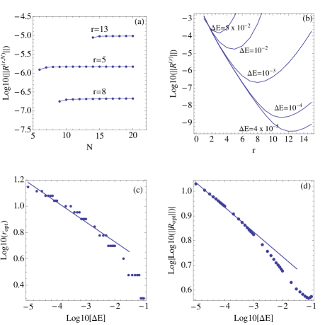
Figure 4: Asymptotic behavior of the non-resonant normal form series exemplified by a specific computation using the norm definition (32) for the remainder function with parameters $\beta=0$, and $E=0.2$. (a) Dependence of the truncated remainder norm on the truncation order $N$ at three different normalization orders $r=5$, $r=8$, and $r=13$, when $\Delta E=0.001$. (b) The quantity $||R^{(r,20)}||$ as a function of $r$ for the indicated values of $\Delta E$. The optimal remainder corresponds to the minimum of each curve. (c) The optimal order as a function of $\Delta E$ in log-log scale. An approximate inverse power-law holds for $\Delta E$ below a threshold $\Delta E\approx 10^{-3}$. The fitting curve corresponds to an exponent 0.15. (d) The value of the optimal remainder (in $\log|\log|$ scale) versus $\Delta E$ (in log scale). The straight line represents an exponential law $R_{opt}\propto\exp((-\Delta E_{0}/\Delta E)^{d})$ with $\Delta E_{0}=10^{-3}$ and $d=0.12$.

To this end, we consider first a norm definition for the remainder series. At the normalization order $r$, the remainder series has the form (setting $\lambda=1$):

$$R^{(r)}(q_{1},q_{2},p_{1},p_{2})=\sum_{s=r+1}^{\infty}H^{(r)}_{s}=\sum_{s=r+1}^{\infty}\sum_{\begin{array}[]{c}{}^{k_{1},l_{1},k_{2},l_{2}>0}\\ {}^{k_{1}+l_{1}+k_{2}+l_{2}=2s+2}\end{array}}G_{s,k_{1},l_{1},k_{2},l_{2}}^{(r)}q_{1}^{k_{1}}p_{1}^{l_{1}}q_{2}^{k_{2}}p_{2}^{l_{2}}~{}~{}.$$ (28)

We define the N-th order truncation of $R^{(r)}$ as

$$R^{(r,N)}(q_{1},q_{2},p_{1},p_{2})=\sum_{s=r+1}^{N}H^{(r)}_{s}=\sum_{s=r+1}^{N}\sum_{\begin{array}[]{c}{}^{k_{1},l_{1},k_{2},l_{2}>0}\\ {}^{k_{1}+l_{1}+k_{2}+l_{2}=2s+2}\end{array}}G_{s,k_{1},l_{1},k_{2},l_{2}}^{(r)}q_{1}^{k_{1}}p_{1}^{l_{1}}q_{2}^{k_{2}}p_{2}^{l_{2}}~{}~{}.$$ (29)

Let now $E,\Delta E$ be fixed such that $0\leq\Delta E<E$. Consider a fixed direction $q_{2}=\beta p_{2}$ in the plane $(q_{2},p_{2})$. It is easy to prove that the quantity

$$||R^{(r,N)}||_{E,\Delta E,\beta} = \sum_{s=r+1}^{N}\sum_{\begin{array}[]{c}^{k_{1},l_{1},k_{2},l_{2}>0}\\ ^{k_{1}+l_{1}+k_{2}+l_{2}=2s+2}\end{array}}\Bigg{(}|G_{s,k_{1},l_{1},k_{2},l_{2}}^{(r)}|((E-\Delta E)/\omega_{1,0}))^{k_{1}+l_{1}\over 2}$$ (32)

$$\times |\beta|^{k_{2}}\left({2\Delta E\over 1+\beta^{2}\omega_{2}^{2}((E-\Delta E)/\omega_{1,0}))}\right)^{k_{2}+l_{2}\over 2}\Bigg{)}$$ (33)

satisfies all the properties of norm definition. The norm (32) provides a measure of the size of the remainder at the given energy levels $E,\Delta E$. In particular, we find the following:

i) For $\Delta E$ sufficiently small, the sequence $||R^{(r,N)}||_{E,\Delta E,\beta}$, for $N=r+1$, $r+2$, $\ldots$ is convergent for, $N\rightarrow\infty$, at all normalization orders $r$. An example is given in Fig.4a. We fix $\beta=0$, $E=0.2$, $\Delta E=0.001$, referring to an estimate of the size of the remainder along the axis $z=0$ on the surface of section of Fig.3a, at a distance $p_{z}=\sqrt{2\Delta E}\approx 4.5\times 10^{-2}$. The behavior of $||R^{(r,N)}||$ is shown for three different normalization orders $r=5$, $r=8$, $r=13$. In all three cases, we find that the norm of the truncated remainder converges rather quickly with the truncation order $N$. This implies that the value of the remainder found at the maximum truncation order $N=20$ used here is a good measure of the limiting value $||R^{(r,\infty)}||$ for all three chosen normalization orders $r$.

ii) Figure 4a provides an indication of the asymptotic behavior of the series for the particular parameters. Namely, we observe that the norm of the remainder decreases as we move from the normalization order $r=5$ to $r=8$, however, it increases as we move from $r=8$ to $r=13$. The dependence of $||R^{(r,N)}||$ on $r$ (fixing $N$ to the maximum $N=20$), for fixed $\beta,E$ is shown in detail in Fig.4b, for five different values of the mirror oscillation energy $\Delta E$. The asymptotic behavior of the remainder series is evident in this plot, which shows also that the optimal order $r_{opt}$, at which the norm of the remainder becomes minimum, decreases as $\Delta E$ increases, while the value of the norm at the optimal order increases with $\Delta E$.

iii) The dependence of $r_{opt}$ on $\Delta E$, shown in Fig.4c is approximately power-law like. The straight line indicates a power law with exponent -0.15 which holds for energies below a threshold value $\Delta E\approx 10^{-3}$. Note that an optimal order as low as $r_{opt}=2$ is reached at the energy $\Delta E\approx 6\times 10^{-2}$. This corresponds to $p_{z}\approx\pm 0.35$ along the axis $z=0$ on the surface of section. Simple visual inspection of Fig.2c shows that this value is close to the border of the stability domain for $z=0$. This suggests that the limits of the stability domain can be estimated analytically by the requirement that $r_{opt}$ becomes very small., e.g. $r_{opt}=2$. Physically, this marks the limit of overall validity of the non-resonant normal form.

iv) The optimal remainder value is exponentially small in $1/\Delta E$. Figure 4d shows the quantity $\log|\log(||R^{(r_{opt},20)}||)|$ vs. $\log\Delta E$ (the value of the remainder decreases for higher values in the ordinate). The straight line corresponds to a law $||R^{(r_{opt})}||\approx\exp(-(\Delta E_{0}/\Delta E)^{d})$ with $d=0.12$. Notice that, as shown also in Fig.4b, the exponential dependence implies that for $\Delta E$ small we can obtain quite small optimal remainder values (e.g. of order $10^{-9}$ when $\Delta E=10^{-4}$, rising to $10^{-4}$ when $\Delta E$ is of order $10^{-2}$. These numbers set the overall level of precision of the non-resonant quasi-integrals as a function of the mirror oscillation energy.

Let us note here that the asymptotic character of the above normal form construction is due to the fact that we seek an expansion in which all quantities are defined in an open domain of the phase space. If, instead, after a few normalization steps, we fix a value of the action $I_{1}=I_{1}*$, and expand locally the Hamiltonian (e.g. Eq.(3.2)) around this value, we can arrive at a form of the normalized Hamiltonian in action-angle variables, allowing for the implementation of the Kolmogorov algorithm of the KAM theorem. The existence of invariant curves in the phase portraits indicates that such a process should yield convergent series on a Cantor set of initial conditions. However, exploring such convergence is beyond the scope of our present study.

4 Resonant normal form

4.1 Bifurcation energy

Resonant periodic orbits $m_{2}/m_{1}$ bifurcate from the central equatorial orbit when $m_{2}/m_{1}=\omega_{2}/\omega_{1}$. Using the non-resonant normal form we can predict the bifurcation energy of the $m_{2}$:$m_{1}$ family. The gyro-frequency of the equatorial orbit $\omega_{1,eq}$ is computed by setting $q_{2}=p_{2}=0$ in the normal form (as in Eq.(3.2)). Then

$$\omega_{1,eq}(I_{1})=\frac{\partial Z(I_{1},q_{2}=p_{2}=0)}{\partial I_{1}}~{}~{}.$$ (34)

The $m_{2}/m_{1}$ family bifurcates at the action value $I_{1}^{*}$ given by:

$$m_{2}\omega_{1,eq}(I_{1}^{*})=m_{1}\omega_{2}(I_{1}^{*})~{}~{}$$ (35)

where $\omega_{2}(I_{1})$ is computed as in Eq.(25). Finally, the bifurcation energy is computed by $E_{m2/m1}=Z(I_{1}^{*})$.

4.2 Algorithm

Denoting $\omega_{1}^{*}=\omega_{1}(I_{1}^{*})$, $\omega_{2}^{*}=\omega_{2}(I_{1}^{*})$, we now construct a resonant normal form for the $m_{2}/m_{1}$ resonance as follows:

i) Book-keeping and Hamiltonian preparation: As long as $I_{1}$ is considered as a small quantity, one has that the quantities $\omega_{1,0}-\omega_{1}=O(I_{1})$, $\omega_{2}^{2}=O(I_{1})$ are also small. Both quantities play the role of ‘detuning’ parameters (Pucacco et al. 2008), since they both represent a difference from the unperturbed frequencies which are $\omega_{1,0}$ and zero respectively. Fixing a value $I_{1}=I_{1}^{*}$, we can formally take this fact into account in the Hamiltonian by adding and substracting the above quantities with a different book-keeping factor, i.e. we set:

$$H=i\omega_{1,0}p_{1}q_{1}+{1\over 2}p_{z}^{2}+...=i\omega_{1}^{*}p_{1}q_{1}+{1\over 2}p_{z}^{2}+{1\over 2}(\omega_{2}^{*})^{2}z^{2}$$

$$-\lambda\left(i(\omega_{1}^{*}-\omega_{1,0})q_{1}p_{1}+{1\over 2}(\omega_{2}^{*})^{2}z^{2}+H_{4}\right)+O(\lambda^{2})$$ (36)

Since $\lambda=1$, nothing has really changed with respect to the original Hamiltonian. However, the second frequency was now explicitly introduced in the zero order Hamiltonian term which is subsequently used in the normal form construction. Furthermore, if $\omega_{1}^{*}$ and $\omega_{2}^{*}$ satisfy a resonant condition, it is possible to proceed with the resonant form of the Birkhoff normal form. We note that the correspondence between book-keeping orders and polynomial degrees is now broken, namely, at the book-keeping order $r$ one has terms of the polynomial degrees $2,4,\ldots,2r+2$. However, this poses no formal obstacles to the construction of the normal form.

The remaining steps in the normal form construction are standard (see Efthymiopoulos 2012 for a review). Introducing the linear canonical change of variables

$$z=\frac{q_{2}+ip_{2}}{\sqrt{2\omega^{*}_{2}}}~{}~{}~{},~{}~{}~{}p_{z}=\frac{\sqrt{\omega^{*}_{2}}(iq_{2}+p_{2})}{\sqrt{2}}$$ (37)

the Hamiltonian becomes of the general form (14) with

$$H_{0}^{(0)}=i\omega^{*}_{1}q_{1}p_{1}+i\omega^{*}_{2}q_{2}p_{2}~{}~{}.$$ (38)

The functions $H^{(0)}_{r}$ contain monomials of the form $q_{1}^{k_{1}}p_{1}^{l_{1}}q_{2}^{k_{2}}p_{2}^{l_{2}}$. The book-keeping rule is $2\leq k_{1}+k_{2}+l_{1}+l_{2}\leq 2r+2$.

ii) Choice of kernel set M. For the resonance $m_{2}/m_{1}$ we set

$${\cal M}_{res}=\left\{(k_{1},k_{2},l_{1},l_{2})~{}\mbox{such that~{}}(k_{1}-l_{1})m_{1}+(k_{2}-l_{2})m_{2}=0\right\}~{}~{}.$$ (39)

This choice ensures that the quantity $I_{res}=i(m_{1}q_{1}p_{1}+m_{2}q_{2}p_{2})$ is a formal integral in the new canonical variables.

iii) Normalization. The normalization proceeds recursively by the same scheme as in subsection 4.1. The functions $\tilde{H}^{(r-1)}_{r}$ denote now the terms of $H^{(r-1)}_{r}$ not belonging to ${\cal M}_{res}$. The homological equation at the r-th step has the form

$$\{i\omega_{1}^{*}q_{1}p_{1}+i\omega_{2}^{*}q_{2}p_{2},\chi_{res,r}\}=-\tilde{H}^{(r-1)}_{r}~{}~{}.$$ (40)

Thus, the equation is diagonal with respect to all monomials belonging to $\tilde{H}^{(r-1)}_{r}$, i.e., for every monomial term $h^{(r-1)}_{k_{1},l_{1},k_{2},l_{2}}q_{1}^{k_{1}}p_{1}^{l_{1}}q_{2}^{k_{2}}p_{2}^{l_{2}}$ in $\tilde{H}^{(r-1)}_{r}$ we add a corresponding term in $\chi_{res,r}$ with coefficient $h^{(r-1)}_{k_{1},l_{1},k_{2},l_{2}}/(i((k_{1}-l_{1})\omega_{1}^{*}+(k_{2}-l_{2})\omega_{2}^{*}))$.

An alternative algorithm to the above would be to introduce a local action variable $J_{1}=I_{1}-I_{1}^{*}$ to be treated as a new small parameter. However, in practice we found that this approach has worse convergence properties than the ones induced by the normal form after the manipulation of the Hamiltonian as in Eq.(4.2). The latter’s efficiency can be tested by numerical examples as below.

4.3 Implementation

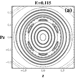
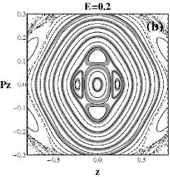
Figure 5: The Poincaré surface of section ($z,~{}p_{z},~{}\rho=0$) (black curves) superimposed with the curves of equal values of the integral of the resonant normal form (gray points) for (a) $E=0.115$ and (b) $E=0.20$. The $3:1$ resonant islands (two sets of 3 islands) in (a) and the $2:1$ resonant islands (two sets of 2 islands) in (b) are very well reproduced by the resonant normal form.

The resonant formal integral $I_{res}$ can be transformed to an expression in the original variables in the same way as for the non-resonant case. After $r$ normalization steps we have

$$\Phi_{res}(q_{1},p_{1},q_{2},p_{2})=\exp(-L_{\chi_{res,1}})\circ\exp(-L_{\chi_{res,2}})\ldots\circ\exp(-L_{\chi_{res,r}})(im_{1}q_{1}p_{1}+im_{2}q_{2}p_{2})~{}~{}~{}.$$ (41)

This allows, again, to compare theoretical with numerical curves on the Poincaré surface of section. Figure 5 shows an example, referring to two different resonances, namely 3:1 (Fig.5a) at the energy $E=0.115$, and 2:1 (Fig.5b), at the energy $E=0.20$, same as in Fig.3b. In both cases, the energy is taken close to but above the bifurcation energy value, which, using the normal form approach (see subsection 4.1) at the 8-th order, is found to be $E_{1/3}=0.097279$ and $E_{1/2}=0.188036$ (the values determined numerically are $E_{1/3}=0.097253$ and $E_{1/2}=0.188015$ respectively). In both cases the resonant normal form represents well the corresponding islands of stability. Furthermore, in both cases the resonant normal form represents also well the invariant curves which surround the center both in the interior and the exterior of the resonant zone. The accuracy of the normal form computations, which depends on the behavior of the remainder of the normal form series as a function of the normalization order, is examined in detail in the next subsection. Here, we emphasize that the overall limit of validity of the resonant normal form approach is defined by the appearance of other resonances, of different order than the resonance under consideration. These extra resonances are conspicuous in the outer parts of the surface of section of Figs.5a,b, where we see also the beginning of a chaotic sea surrounding the main domain of stability.

4.4 Asymptotic behavior

The asymptotic behavior of the resonant normal form is probed again by numerical experiments, in the same way as in subsection 4.3 for the non-resonant normal form. Here, since both frequencies $\omega_{1}^{*}$ and $\omega_{2}*$ are fixed, we introduce a slight modification of the norm definition with respect to Eq.(32), taking into account also the different choice of book-keeping rule. Thus, we set:

$$||R^{(r,N)}||_{E,\Delta E,\beta} = \sum_{s=r+1}^{N}\sum_{\begin{array}[]{c}^{k_{1},l_{1},k_{2},l_{2}>0}\\ ^{k_{1}+l_{1}+k_{2}+l_{2}=2,4,\ldots 2s+2}\end{array}}\Bigg{(}|G_{s,k_{1},l_{1},k_{2},l_{2}}^{(r)}|((E-\Delta E)/\omega_{1}^{*}))^{k_{1}+l_{1}\over 2}$$ (44)

$$\times |\beta|^{k_{2}}\left({2\Delta E\over 1+\beta^{2}(\omega_{2}^{*})^{2}((E-\Delta E)/\omega_{1}^{*}))}\right)^{k_{2}+l_{2}\over 2}\Bigg{)}~{}~{}.$$ (45)

Figure 6, which is quite similar to Fig.4, clearly shows that the resonant normal form series exhibit asymptotic properties analogous to the non-resonant one. Nevertheless, a comparison of Figs. 4b and 6b shows that the overall error of the resonant formal integrals is uplifted by about one order of magnitude with respect to the non-resonant case for similar levels of mirror oscillation energy $\Delta E$. The exponent found in Fig. 8c is also close to 0.2. Finally, we observe that the exponential regime for the scaling of the optimal remainder with $1/\Delta E$ holds for mirror oscillation energies below a value $\Delta E\leq 10^{-3}$.

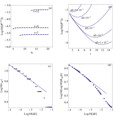
Figure 6: Asymptotic behavior of the resonant normal form. (a-d) Same as in Fig.4a-d, but for the resonant normal form computation with parameters as indicated in the figure. The norm definition is given in Eq.(44).

4.5 Normal form determination of the threshold to global chaos

The domain of regular motion around the central periodic orbit shrinks, in general, as the energy increases. This domain shrinks to zero at an energy $E_{t}$ where the central orbit exhibits (for the first time) a transition from stability to instability. The energy $E_{t}$ can be found numerically by computing the monodromy matrix of the central periodic orbit at different energies. Numerically, we find $E_{t}=E_{1}\approx$0.36688.

The energy $E_{t}$ marks the limit of applicability of the normal forms in magnetic bottle problem, in either the non-resonant or resonant form. We show now how the energy $E_{t}$ can be determined by normal form computations. We proceed as follows: at the energy $E=E_{t}$, the two frequencies $\omega_{1}$ and $\omega_{2}$ become equal (Contopoulos, 1968). We then have the bifurcation of two equal period resonant periodic orbits from the central orbit. Thus we have $E_{t}=E_{1/1}$. However, $E_{1/1}$ can be computed as indicated in subsection 4.1, for the resonance $m_{1}=m_{2}=1$.

The accuracy of the theoretically computed value depends on the normalization order $r$. Fig.7a shows the frequencies $\omega_{1}$ and $\omega_{2}$ as functions of the energy $E$ using the normal form at the normalization order $r=10$. The intersection point of the two curves yields a theoretical estimate $E_{t}$=0.39550, which has an error $\delta E\approx$0.0286. The error is reduced as $r$ increases. Figure 7b shows the estimate for $E_{t}$ as a function of $r$ up to $r=30$. The convergence to the numerically computed value is rather slow, the error being about $10^{-2}$ at $r=30$.

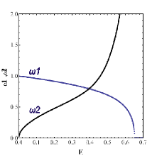
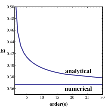
Figure 7: (a) Theoretical values for the frequencies $\omega_{1}$ and $\omega_{2}$ as functions of the energy $E$ by the normal form at the normalization order $r=10$. The intersection point yields an estimate of the energy $E_{t}$ where the first transition of the central periodic orbit from stability to instability takes place. (b) The theoretical estimate $E_{t}$ as a function of the normalization order $r$. The horizontal line corresponds to the numerically computed value of $E_{t}$.

5 Conclusions

In the present paper we explored the limits of applicability of the normal form theory in a polynomial magnetic bottle Hamiltonian model. We focused on a new algorithm for the construction of the normal form and the computation of quasi-integrals (truncated formal integrals) in cases of resonance between the gyration and the mirror frequencies. Furthermore, we explored the asymptotic behavior of both the non-resonant and the resonant normal form series. Our main conclusions can be summarized as follows:

1) We explored the asymptotic behavior of the non-resonant normal form series. Extending the computations at high normalization series confirms the basic theoretical picture that the behavior of the normalization is asymptotic. Namely, although the size of the remainder of the normal form series goes to infinity when the normalization order $r$ tends to infinity, we observe that initially (at low order $r$) the size of the remainder decreases with $r$. The remainder becomes minimum at an optimal order $r$ which scales approximately as an inverse power of the mirror oscillation energy $\Delta E$. The size of the optimal remainder is found to be exponentially small in $1/\Delta E$. We estimate numerically the exponents related to this asymptotic behavior.

2) The non-resonant normal form allows to compute theoretically the energies at which resonant periodic orbits of any resonance $m_{2}:m_{1}$ (between the mirror and the gyration frequencies, with $m_{1},m_{2}$ integers) bifurcate from a ‘central’ (equatorial) orbit. We propose a novel computation of the normal form in the case of resonances. This is based on combining two algorithmic techniques called ‘detuning’ (Pucacco et al. 2008) and ‘book-keeping’ (Efthymiopoulos 2012). We give numerical examples of applicability of the resonant formal series in the case of the 3:1 and 2:1 resonances, and demonstrate their ability to predict the form of the phase portrait in the neighborhood of each resonance.

3) We explore the asymptotic behavior also of the resonant formal series, which is found to be qualitatively similar to the non-resonant case, and estimate numerically the associated exponents.

4) The suggested normal form computations serve to predict two results regarding the onset of chaos. i) At low energies, one can estimate the limits of the domain of stability around the central equatorial orbit, i.e. how far from this orbit (in phase space) does chaos become important. ii) The onset of global chaos can be approximated by the energy value where the central orbit suffers its first transition from stability to instability, which coincides with the bifurcation energy of the 1:1 resonance.

References

- [1] Arnold, V.I., Kozlov, V.V. and Neishtadt, A.I. : 1988, ”Mathematical Aspects of Classical and Celestial Mechanics”, Springer, Berlin .
- [2] Baider, A., and Sanders, J.A.: 1991, J. Diff. Eq. 92, 282.
- [3] Benettin, G. and Sempio, P.: 1994, Nonlinearity 7, 281.
- [4] Benettin, G., Henrard, J. and Kuskin, S. : 1999, ”Hamiltonian Dynamics. Theory and Applications”, Springer, Berlin.
- [5] Churchill R.C., Pecelli G. and Rod D.L.: 1980, Arch. for Rat. Mech. and Anal. 73, 313.
- [6] Contopoulos G.:1965, Astrophys. J., 142, p.802.
- [7] Contopoulos G.: 1968, Astrophys. J. 153, 83.
- [8] Contopoulos, G. and Harsoula, M.: 2008, Int. J. Bif. and Chaos, 18, 2929
- [9] Contopoulos, G. and Harsoula, M.: 2010a, Cel. Mech. Dyn. Astron., 107, 77.
- [10] Contopoulos G. and Harsoula M.: 2010b, Int. J.Bif. and Chaos 20, 2005.
- [11] Contopoulos, G. and Vlahos, L.: 1975, J. Math. Phys., 16, 1469.
- [12] Contopoulos, G. and Zikides, M.: 1980, Astron. Astroph., 90, 198.
- [13] Cushman, R., and Sanders, J.A.: 1986, in M. Golubitsky and J. Guckenheimer (eds), Amer. Math. Soc. Contemporary Mathematics, 56, Providence, RI.
- [14] Dendy, R.O.: 1993, ‘Plasma Physics: an introductory course’, Cambridge University Press, Cambridge, UK.
- [15] Dragt, A. J.: 1965, Rev. Geophys. Space Phys., 3, 255.
- [16] Dragt, A. J. and Finn, J. M.: 1979, J. Math. Phys., 20, 2649.
- [17] Dunnett, D.A., Laig, E.W. amd Taylor, J.B.: 1968, J. Math. Phys., 9, 1819.
- [18] Efthymiopoulos, C.: 2008, Cel. Mech. Dyn. Astron., 102, 49.
- [19] Efthymiopoulos, C.: 2012, in Cincotta, P., Giordano, C. and Rfthymiopoulos, C. (eds) ”Chaos, diffusion and non-integrability in Hamiltonian systems- Applications to Astronomy”, Asocation Argentina de Astronomia Workshop Series, 3, p.3-146.
- [20] Efthymiopoulos, C., Giorgilli, A. and Contopoulos , G.: 2004, J. Phys. A, 37, 10831.
- [21] Elphick, C.: 1988, J. Phys. Lett. A, 127, 418.
- [22] Engel, U., M., Stegemerten, B. and Eckelt, P.: 1995, J. Phys. A, 28, 1425.
- [23] Gurnett, D.A., and Bhattacharjee, A.: 2005, ‘Introduction to Plasma Physics: With Space and Laboratory Applications’, Cambridge University Press, Cambridge, UK.
- [24] Harsoula M., Kalapotharakos C. and Contopoulos G.: 2011, Int. J. Bif. and Chaos, 21, 2221.
- [25] Howard, J.: 1970, Physics of Fluids, 13, 2407.
- [26] Jackson, J,D.: 1962, ”Classical Electrodynamics”, Wiley , New York.
- [27] Kruskal M.: 1962, J. Math. Phys. 3, 806
- [28] Lichtenberg A.J. and Lieberman M.A.: 1992, ”Regular and Chaotic Dynamics”, Springer-Verlag, 1992.
- [29] McNamara, B.:1978, J. Math.Phys. 19, 2154.
- [30] Meyer, K.R.:1984, Funk. Ekvacioj 27, 261.
- [31] Neishtadt, A.I.: 1981, J. Applied Math. Mech. 45, 58.
- [32] Neishtadt, A.I.: 1984, J. Applied Math. Mech. 48, 197.
- [33] Northrop, T.G.: 1964, ”The adiabatic motion of charged particles”, Wiley, London.
- [34] Pucacco, G., Boccaletti, D. and Belmonte C.: 2008, Cel. Mech. Dyn. Astron., 102, 163
- [35] Sanders, J.A., Verhulst, F., and Murdock, J.: 2007, ‘Averaging Methods in Nonlinear Dynamical Systems’, Springer, Berlin.