Turnplate of quantum state

Abstract

Time-reversal symmetry breaking can enhance or suppress the probability of success for quantum state transfer (QST), and remarkably it can be used to implement the directional QST. In this paper we study the QST on a ring with time-reversal asymmetry. We show that the system will behave as a quantum state turnplate under some proper parameters, which may serve as time controlled quantum routers in complex quantum networks. We propose to to realize the quantum state turnplate in the coupled resonator optical waveguide by controlling the coupling strength and the phase.

I Introduction

Quantum state transfer (QST) is one of the basic tasks in quantum information process. In the past decade QST has been studied intensively. Several schemes are proposed to achieve it by different channels, i.e., spin chains Bose (2003); Christandl et al. (2004); Yao et al. (2011, 2012); Li et al. (2005), polarized photons in the optical fiber Cirac et al. (1997); Ritter et al. (2012), coupled-cavity array and so on. Based on cavity quantum electrodynamics a scheme is to transfer the state of a qubit from a cavity-atom system to another one through an optical fiber connecting the two cavities. Using the spin chain as a channel many schemes are reported, such as, QST along a one dimensional unmodulated spin chain Bose (2003), perfect QST achieved by modulating the coupling strength Wójcik et al. (2005); Campos Venuti et al. (2007); Li et al. (2005); Giampaolo and Illuminati (2010); Gualdi et al. (2008); Yao et al. (2011); Bruderer et al. (2012), QST without initialization Di Franco et al. (2008); Markiewicz and Wieśniak (2009), optimizing basis Bayat et al. (2011); Liu et al. (2013) and generalizing to the high spin QST Bayat and Karimipour (2007); Qin et al. (2013); Bayat (2014). Other schemes, such as, transferring single-mode photon state through a coupled-cavity array, are also reported. Recently time-reversal symmetry breaking is introduced to study the QST Zimborás et al. (2013); Lu et al. (2014), where the time-reversal symmetry breaking can enhance or suppress the probability of the QST and make the QST directional bias. In this sense time asymmetry is a new resource for exploring the QST.

In Refs. Hafezi et al. (2011, 2013), it is shown that a synthetic magnetic field can be introduced for photons by differential optical paths in system of the coupled resonator optical waveguides (CROW). In this paper we consider the QST along a ring consisting of coupled cavities or coupled resonator optical waveguides with time reversal asymmetry. Because of the time reversal symmetry breaking we hope that the quantum state transfer along the ring one by one periodically like a turnplate of quantum states. The quantum turnplate will be useful in building complex quantum networks where it acts as a quantum router. In the following of the paper we show that a CROW ring will behave as quantum state turnplate under some proper parameters.

This article is organized as follows. First we give the physical model and make a general analysis. Then, we analyze the dynamic requirement for the quantum state turnplate in a single excitation model, and give the energy spectrum and symmetry matching condition for quantum state turnplate. In Sec. IV, we study the spectrum of the system with the $c_{n}$ symmetry. Then, we discuss the effective Hamiltonian of the system using perturbation method. We come back to the CROW system in Sec. VI. Finally a summary is given.

II Physical model

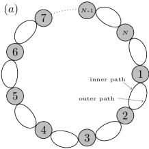
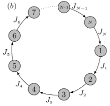
Figure 1: (a) The CROW ring. The circles mean the site resonators, and the link optical waveguides link the resonators as a ring. Every waveguide between two site resonators has two paths, the outer path and the inner path. The two paths have different length which induce the complex coupling strength $J$. (b) Single excitation graph. The circles correspond to the resonators in CROW system. The arrow with labels $J_{l}$ represents the matrix element $J_{l}|l\rangle\langle l+1|$.

In the CROW the synthetic magnetic field can be introduced by differential optical paths Hafezi et al. (2011, 2013). We consider the CROW system in a ring configuration as shown in Fig. 1(a). The Hamiltonian of the ring is

$$H_{R}=\sum_{l=1}^{N}(J_{l}\hat{a}_{l}\hat{a}^{\dagger}_{l+1}+J_{l}^{\ast}\hat{a}^{\dagger}_{l}\hat{a}_{l+1}),$$ (1)

where $J_{l}$ is the coupling strength of between the sites $l-1$ and $l$, and $N+1$ is interpreted as $1$. $\hat{a}_{l}$ ($\hat{a}_{l}^{\dagger}$) is the annihilation (creation) operator. From Ref. Liu and Zhou (2015) we know that the condition for transferring any single mode photon state from node $l$ to node $l^{\prime}$ is

$$\hat{a}_{l^{\prime}}(\tau)=\hat{a}_{l},$$ (2)

where $\hat{a}_{l^{\prime}}(\tau)=U^{\dagger}(t)\hat{a}_{l^{\prime}}U(t)$ with $U(t)$ being the time evolution operator. It can be easily verified by noting that the expect value of any operator in the $l^{\prime}$-th node at time $\tau$ is equal to that of the operator in the $l$-th node in the initial state.

Using the Heisenberg equation

$$\frac{d\hat{a}_{l}(t)}{dt}=i\left[H_{R},\hat{a}_{l}(t)\right]$$ (3)

and noting that $\hat{a}_{l}(t)$ can be expressed on the operator bases as

$$\hat{a}_{l}(t)=\sum_{k=1}^{N}\alpha_{k}(t)\hat{a}_{k},$$

the evolution of the operator $\hat{a}_{l}(t)$ can be written as

$$i\frac{dA}{dt}=-H(J)A,$$ (4)

where $A={[\alpha_{1}(t),\,\alpha_{2}(t),\,\ldots,\alpha_{N}]}^{T}$ with $T$ being the transpose operation, and

$$H(J)=\begin{bmatrix}0&J_{1}&0&\cdots&J_{N}^{*}\\ J_{1}^{*}&0&J_{2}&\cdots&0\\ 0&J_{2}^{*}&0&\cdots&0\\ \vdots&\vdots&\vdots&\ddots&\vdots\\ J_{N}&0&0&\cdots&0\end{bmatrix},$$ (5)

The initial condition is $A(0)={[0,\,0,\,\ldots,1,\ldots,0]}^{T}$, where $1$ is the $l$-th element. With the above initial condition, Eq. (4) describes the single excitation evolution in the ring with coupling strength $\{-J_{i}\}$.

So the transfer of any single mode photon state in the CROW ring has the same physical picture as the single excitation model, and we do not need to initialize the state of other sites except the input one.

III Single excitation ring

Firstly, we consider the single excitation model. To sketch our central idea, we consider the system depicted by a graph in Fig. 1(b) consisting of $N$ sites as a ring, with the Hamiltonian $H(J)$ having the form given in Eq. (5), where $J$ is the the set $\{J_{l}\}$. Let us denote $\Phi$ as the set $\{\phi_{l}\}$, where $\phi_{l}$ is the complex phase of $J_{l}$. From Ref. Lu et al. (2014) we know that the phase $\Phi$ can give rise to the time-reversal asymmetry if the graph is non-bipartite graph ($N$ is odd). In this article we concentrate on the cases where $N$ is odd.

Through local unitary operator $U^{L}$, the Hamiltonian can be transformed to

$$H(J^{\prime})=U^{L}H(J)U^{L\dagger},$$

where $\sum_{l}\phi^{\prime}_{l}=\sum_{l}\phi_{l}$ and $|J^{\prime}_{l}|=|J_{l}|$. In other words, only the sum of phases $\sum_{l}\phi_{l}$ is relative to the properties of QST. So we can choose a proper operator $U^{L}$ to make all the phases equal, $\phi_{l}^{\prime}=\frac{\sum_{l}\phi_{l}}{N}$, with the QST properties in the time evolution unchanged.

Now we consider the question: In what condition would the system behave like a turnplate of quantum state? Firstly, we require that the system have the symmetry of the cyclic group, $c_{n}$, for the turnplate having $n$ ($n\leq N$) scales on it, i.e. $N/n$ is an integer. The operators of the $c_{n}$ group elements can be expressed as

$$\mathcal{T}_{n},\,{(\mathcal{T}_{n})}^{2},\,\ldots,\,{(\mathcal{T}_{n})}^{n-1},\,1$$

where

$$\mathcal{T}_{n}=e^{iL_{n}\frac{2\pi}{n}}$$

and $L_{n}$ is a Hermitian operator. From ${(\mathcal{T}_{n})}^{n}=1$, we know that $L_{n}$ has $n$ integer eigenvalues, $l\in\{\lfloor-\frac{n-1}{2}\rfloor,\,\lfloor-\frac{n-1}{2}\rfloor+1,\ldots,\,\lfloor\frac{n-1}{2}\rfloor\}$ ，where $\lfloor x\rfloor$is the largest integer not greater than $x$. Here we only consider the case where $n$ is odd. For the Hamiltonian we have the relation $[H,\,L_{n}]=0$. Let the eigenstate of the system be $\left|\psi_{l,m}\right>$, that is

$$H|\psi_{l,m}\rangle=E_{l,m}|\psi_{l,m}\rangle,$$

and

$$L_{n}|\psi_{l,m}\rangle=l|\psi_{l,m}\rangle.$$

Now we prove that the system will be a turnplate of quantum states with $n$ scales if the eigenvalues $E_{l,m}$ match the symmetry $c_{n}$ in the following way:

$$E_{l,m}=\left(\frac{l}{n}+Z_{m}\right)\epsilon+\epsilon_{0},$$ (6)

where $Z_{m}$ is an integer, and $\epsilon_{0}$ correspond to the phase that is not an observable in physics.

Let the initial state of the system is $|\psi_{0}\rangle$. It can be easily proved that at time $\tau=\frac{2\pi}{\epsilon}$,

$$|\psi(\tau)\rangle=e^{i\pi\epsilon_{0}/\epsilon}\mathcal{T}_{n}|\psi_{0}\rangle,$$ (7)

meaning that quantum state of the system turn one scale every time interval $\tau$. The energy and symmetry matching condition can be seen as the generalization of the energy and parity matching condition mentioned in Ref. Shi et al. (2005), where the parity matching condition corresponds to the case $n=2$ and $\epsilon=2E_{0}$.

Here we look at the particular case $N=n=3$. The relation $[H,\,\mathcal{T}_{3}]=0$ requires that $J_{1}=J_{2}=J_{3}$. $l\in\{0,\,\pm 1\}$ and using the property of the $c_{3}$ group we known $H$ and $L_{n}$ have the same eigenvectors $|\phi_{l}\rangle=\frac{1}{\sqrt{3}}{[1,\,\omega_{3}^{l},\,\omega_{3}^{2l}]}^{T}$ with $\omega_{3}=e^{i\frac{2\pi}{3}}$. When $J_{1}=J_{2}=J_{3}=e^{i\frac{\pi}{6}}$, that is the total phase is $\pi/2$, the eigenvalues are $E_{l=0}=\sqrt{3}$, $E_{l=1}=-\sqrt{3}$, $E_{l=-1}=0$. So we get $\epsilon_{0}=\frac{\epsilon}{3}=\sqrt{3}$ and the time interval is $\tau=\frac{2\pi}{3\sqrt{3}}$. We numerically stimulate the time evolution of this case and show the probability of the wave function in the Fig 2.

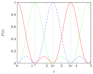
Figure 2: (Color online) Numerical stimulation of the time evolution of the system consisting of 3 sites with the parameters $J_{1}=J_{2}=J_{3}=e^{i\frac{\pi}{6}}$ and the initial state $|100\rangle$. $P(t)$ is the probability of the wave function. The solid line, dashed line and dashdotted line describe the probability at site 1, site 2 and site 3 respectively. At time $\tau$ the excitation transfers from site 1 to site 2 and it transfers to site 3 after a next time interval $\tau$. The system acts like a turnplate of the excitation.

Given the single excitation condition, it was proved that there is the pretty good state transfer between any two sites of a uniform ring with total phase as $\pi/2+k\pi$, if the number of the site of the ring is prime, in Ref. Cameron et al. (2014). It indicates that the energy spectrum and symmetry matching condition, Eq. (6) is approximately satisfied when the length of the ring is prime.

IV structure of the spectrum

In this section we analyze the energy spectrum of the system described by the Hamiltonian in Eq. (5). We start with the definitions of some notations. We denote the characteristic polynomial as $A_{N}$, that is $A_{N}=\det(H_{N}-\lambda)$. And denote $B_{N}$ as $B_{N}=\det(H_{N}(J_{N}=0)-\lambda)$, where $H_{N}(J_{N}=0)$ represents the Hamiltonian where the coupling between first site and the last site is zero, i.e., the chain is an open one. From the Ref. Liu and Zhou (2014) we know that,

$$B_{N}=\begin{cases}\lambda g(\lambda^{2})&\text{ if }N\text{ is odd,}\\ g(\lambda^{2})&\text{ if $N$is even, }\end{cases}$$

where $g\left(x\right)$ is an arbitrary function of $x$. So the determinate of $A_{N}$ with odd $N$ is

$$\det A_{N} =-\lambda\det B_{N-1}-J_{1}^{2}\det B_{N-2}$$

$$\ \ \ +\prod_{l=1}^{N}J_{l}e^{i\phi}+\prod_{l=1}^{N}J_{l}e^{-i\phi}-J_{N}^{2}\det B_{N-2}$$

$$=\lambda f(\lambda^{2})+\lambda g(\lambda^{2})+2\prod_{l}J_{l}\cos\phi$$

$$=\lambda F(\lambda^{2})+\prod_{l}J_{l}2\cos\phi，$$

where $\phi$ is the total phase. When $\phi=\frac{\pi}{2}+k\pi$, $k=0,\,\pm 1,\,\pm 2,\,\cdots$, the spectrum has the structure $\{0,\,\pm E_{l}\}$ that is the spectrum is symmetric around $0$. Let us consider the system that has the $C_{n}$ symmetry and contains $N=n\times p$ sites. The eigenvalues of the operator $L_{n}$ is $0,\,\pm 1,\,\ldots,\,\pm\frac{n-1}{2}$, which we label as $l$, and every eigenvalue has $p$-fold degeneracy. We can easily write out the eigenvector of $L_{n}$,

$$|l,\,i\rangle =\frac{1}{\sqrt{n}}\left(|i\rangle+\omega_{n}^{l}|i+p\rangle+\omega_{n}^{2l}|i+2p\rangle\right.$$

$$\left.+\cdots+\omega_{n}^{(n-1)l}|i+(n-1)p\rangle\right).$$

Let $P_{l}=\sum_{i}|l,i\rangle\langle l,i|$. From the relation $[H,\,L]=0$, we know that

$$P_{l}HP_{l^{\prime}} =0 \ \ \ for\text{ }l\neq l^{\prime}.$$

This means that the Hamiltonian is block diagonalized under the bases $\{|l,\,i\rangle\}$. Because the system has the $c_{n}$ symmetry, we have the relation $J_{i}=J_{i+p}$. So there are only $p$ parameters, $J_{1},\,J_{2},\,\ldots,\,J_{p}$. We can always let $J_{1}=1$ and other parameters be the ratio to $J_{1}$. Then the property of the system don’t change up to the time scales. So there are $p-1$ parameters that we need to consider.

Using the bra ket form of the Hamiltonian

$$H =J_{N}|N\rangle\langle 1|+J_{N}^{*}|1\rangle\langle N|$$

$$\ \ \ +\sum_{k=1}^{N-1}\left(J_{k}|k\rangle\langle k+1|+J_{k}^{*}|k+1\rangle\langle k|\right),$$ (8)

and acting the projector $P_{l}$ on both sides of Eq. (8) we can directly give

$$P_{l}HP_{l} =\omega_{n}^{l}J_{p}|p\rangle\langle 1|+\omega_{n}^{l*}J_{p}^{*}|1\rangle\langle p|$$

$$\ \ \ +\sum_{k=1}^{p-1}\left(J_{k}|k\rangle\langle k+1|+J_{k}^{*}|k+1\rangle\langle k|\right).$$ (9)

Comparing Eq. (8) and Eq. (9) we get that in the every block the Hamiltonian is equivalent to the Hamiltonian of the ring with length $p$ and the moduli of the coupling strength are not changed just with the total phase changing from $\phi/n$ to $\phi_{l}=\frac{\phi}{n}+\frac{2l\pi}{n}$, see Fig. 3. So the characteristic function can be written as

$$\lambda F(\lambda^{2})+2\prod_{k=1}^{p}J_{k}\cos\phi_{l}=0,$$

where $l=-\frac{n-1}{2},\,\ldots,\,\frac{n-1}{2}$. Every function means a curve that cross with the axis of the variable $p$ times corresponding to the $p$ roots, see Fig. 4(a). All the curves have the same shape. When the total phase $\phi=\frac{\pi}{2}+k\pi$, the curve corresponding to $l=-\frac{n+1}{4}$ (or $l=\frac{n-1}{4}$) crosses the original point and we call it curve-$0$. Other curves can be got from the curve-$0$ by translate $2\prod_{k}J_{k}\cos\phi_{l}$ along the vertical axis. So if $\prod_{k=1}^{p}J_{k}$ are little enough the spectrum of the Hamiltonian has the shape indicated in Fig. 4(b), that is, the spectrum consists of separated groups.

Figure 3: The ring with $9$ nodes and $c_{3}$ symmetry. Under the bases $|l,i\rangle$ the Hamiltonian is block diagonalized consisting $3$ blocks which is implied by $c_{3}$. In every block the Hamiltonian represents an ring with length $3$ and the coupling strength is the same as the original ring in the site bases with the total phase being $\phi/3$, $\phi/3+2\pi/3$ and $\phi/3+4\pi/3$ where $\phi$ is the total phase of the original ring.

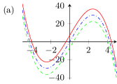
Figure 4: Spectrum structure of the Hamiltonian $H_{9}$ with length $N=9$ and $C_{3}$ symmetry. The coupling strength is $J_{1}=J_{3}=e^{\frac{\pi}{18}}$, $J_{2}=4J_{1}$. So the total phase is $\phi=\pi/2$. (a) Pictures of the characteristic polynomials of three equivalent Hamiltonians got from the Hamiltonian $H_{9}$. The dashdotted line is the curve-$0$ corresponding to $l=-1$, and the other two lines can be got from curve-$0$ by translated along the vertical axis. (b) Spectrum of the Hamiltonian $H_{9}$. Every energy elver correspond to one cross point of the curve and the horizontal axis in (a).

V Effective Hamiltonian

Now we introduce the approximate method based on the spectrum structure. To discuss concretely, we consider the system with nine sites ($N=9$) and the $c_{3}$ symmetry. Its configure is shown in Fig. 3. The eigensystem of the Hamiltonian $H$ is equivalent to the Hamiltonian $H^{\prime}$ with

$$J^{\prime}_{k}=|J_{k}|,\text{ for }k\neq 1$$

$$J^{\prime}_{1}=|J_{1}|e^{i\phi},$$

where $\phi=\sum_{k}\phi_{k}$. So we consider the Hamiltonian $H^{\prime}$. Let $J_{2}^{\prime}\gg J_{1,3}^{\prime}$ and write the Hamiltonian $H^{\prime}$ into two terms, $H^{\prime}=H^{\prime}_{0}+V$. Given that the $H^{\prime}$ is represented in the site basis $|i\rangle$, $H^{\prime}_{0}$ consists of the terms containing $J_{2}^{\prime}$ , and $V$ consists the terms containing $J^{\prime}_{1,3}$. $V$ is the perturbation compared with $H_{0}^{\prime}$.

The eigenvalues of the Hamiltonian $H^{\prime}_{0}$ are $\alpha\in\{0,\,\pm J_{2}^{{}^{\prime}}\}$ and every energy level has three-fold degeneracy. So the energy levels are separated into three groups (manifold) corresponding to three $\alpha$s. Using $i$ label the different bases we denote the three manifold as $|i,\,\alpha\rangle$. In the manifold with $\alpha=0$ the three bases are

$$|1\rangle,\,|4\rangle,\,|7\rangle.$$

And the manifolds with $\alpha=\pm|J_{2}|$ are spanned by the bases

$$|X_{23}^{+}\rangle,\,|X_{56}^{+}\rangle,\,|X_{89}^{+}\rangle$$

and

$$|X_{23}^{-}\rangle,\,|X_{56}^{-}\rangle,\,|X_{89}^{-}\rangle$$

respectively, where

$$|X_{ij}^{+}\rangle=\frac{|0\rangle_{i}+|1\rangle_{j}}{\sqrt{2}},\text{ and }|X_{ij}^{-}\rangle=\frac{|0\rangle_{i}-|1\rangle_{j}}{\sqrt{2}}.$$

We take $V$ as perturbation then compute the effective Hamiltonian in the manifold $\alpha=0$. And the effective Hamiltonian is

$$H_{\rm eff}^{\alpha=0}=-\begin{bmatrix}0&ge^{i\phi}&g\\ ge^{-i\phi}&0&g\\ g&g&0\end{bmatrix},$$

where $g=\frac{J_{1}J_{3}}{J_{2}}$. $H_{\rm{eff}}^{\alpha=0}$ is identical to the representation of the Hamiltonian of the ring consisting of three nodes with uniform coupling strength $g$ and total phase $\phi$. From the analysis in the Sec. III we know that when $\phi=\frac{\pi}{2}+k\pi$ the system is a turnplate of quantum state with three scales and the time interval of transfer state from one node to next is $\frac{2\pi}{3g\sqrt{3}}$. We numerically simulate the time evolution of the system with parameters $J_{1}=J_{3}=1$, $J_{2}=100$ and $\phi=-\frac{\pi}{2}$ from the initial state $|\psi(0)\rangle=|1\rangle$ in Fig. 5. At time $\tau=120.92$ the excitation transfer from site $1$ to site $4$ and after the same time interval it transfer to site $7$ then back to site $1$ circularly. The sites except the sites $1$, $4$ and $7$ can’t be excited.

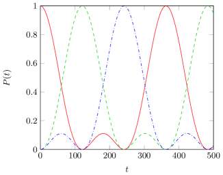
Figure 5: (Color online) Numerically simulate the time evolution of the system with 9 sites. $J_{1}=J_{3}=1$, $J_{2}=100$ and $\phi=-\frac{\pi}{2}$. The initial state is $|\psi(0)\rangle=|100000000\rangle$ with $|1\rangle$ as input state. Solid line presents the fidelity of the state transfer for the state of the first site at different time. The dashed line and the dashdotted line corresponding to the fidelity for the seventh site and fourth site respectively.

The correspondence between the propriety of the system with site number $N=n\times p$ and $N=n$, where $n$ is decided by the symmetry of the large system, can be generalized to general case. Let $J_{1(p)}\ll J_{l\neq 1(p)}$ then the Hamiltonian can be written as $H=H_{0}+V$, where $V$ is perturbation term consisting of the terms containing $J_{1(p)}$, and $H_{0}$ is other terms. The spectrum of the Hamiltonian $H_{0}$ has the form depicted in Fig. 6. The zero energy level is $n$-fold degeneracy with degenerate ket $|m^{(0)}\rangle$, where $m=1+l\times p$ and $l=1,2,\ldots,n-1$. All the $|m\rangle$s span the manifold $\mathcal{M}_{\alpha=0}$. The energies greater and less than zero distribute two sides of the zero energy level symmetrically with an energy gap and every energy level is $n$-fold degeneracy. From the perturbation theory in the degenerate case we know that up to the first order the eigenkets of Hamiltonian $H$ corresponding to the manifold $\mathcal{M}_{\alpha=0}$ are

$$|\phi\rangle=\sum_{m}c_{m}|m\rangle-\sum_{k\notin\mathcal{M}}\frac{|k^{(0)}\rangle V_{k,m}}{E_{k}^{(0)}},$$

where $V_{k,m}=\langle k|V|m\rangle$ and $|k^{(0)}\rangle$ is the eigenket of $H_{0}$ which is not in the manifold $\mathcal{M}_{\alpha=0}$. So when $V_{k,m}$ is much less than $E_{k}^{(0)}$ (the gap on the zero energy level), the manifold $\mathcal{M}_{\alpha=0}$ is close, i.e., if the initial state is $|m\rangle$ then the system is govern by the effective Hamiltonian $H_{eff}^{\alpha=0}$ which represents a Hamiltonian of the $n$-site cycle. So the system with $N=n\times p$ and $c_{n}$ symmetry can be reduced to the system with $N=n$ and with $c_{n}$ symmetry.

Figure 6: Spectrum of the $H_{0}$ which is the main part of the Hamiltonian. Every zero energy level denotes the Hilbert space of the sites labeled by number $(1+l\times p)$, and every grouped $p-1$ levels denote the Hilbert space of the sites form $(2+l\times p)$ to $p+(l\times p)$ respectively, where $l=0,1,\ldots,n-1$.

VI Quantum turnplate on the CROW ring

Now we come back to the physical system, the CROW ring. For the ring containing three resonators, they can be connected by three identical connecting waveguides, which contribute the same coupling strength $|J_{l}|$ and phase $\phi_{l}$. In order to make a quantum turnplate we just need to modify the optical path to make total phase $\phi=\pi/2+k\pi$. Initially we input the photonic state to the node 1. Then we will see that the photonic state will transfer from node 1 to node 2, node 3 and back to node 1 cyclicly with perfect fidelity every time interval $\tau$. For the ring contains $N=3\times p$ resonators, which has the $c_{3}$ symmetry, we need to modify the coupling strength between resonators and connecting waveguides to satisfy the condition $J_{1(p)}\ll J_{l\neq 1(p)}$ and change the optical path to make the total phase be $\phi=\pi/2+k\pi$. Then photonic states can be transfer among the site $1$, $p+1$, and $2p+1$ cyclicly with high fidelity.

We simulate the QST along the CROW ring consisting 9 resonators with $c_{3}$ symmetry. The parameters are $|J_{1}|=|J_{3}|=1$, $|J_{2}|=100$ and the total phase $\phi=\pi/2$. Initially the state $|\psi\rangle=(|0\rangle+|1\rangle+|2\rangle)/\sqrt{3}$ is input into the first resonator. Then we observe transfer of $|\psi\rangle$ along the ring. In Fig. 7 we plot the time evolution of the fidelity

$$F(t)=\langle\psi|\rho_{i}(t)|\psi\rangle$$

of sites $1$, $4$ and $7$ and it behaves as a quantum state turnplate. $\rho_{i}$ means the reduced density matrix of site $i$.

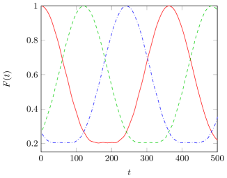
Figure 7: (Color online) Numerically simulate the time evolution of the fidelity of the CROW system with 9 resonators. $J_{1}=J_{3}=1$, $J_{2}=100$ and $\phi=\frac{\pi}{2}$. The initial state is $\frac{1}{\sqrt{28}}(|0\rangle+2|1\rangle+3|2\rangle)(|1000000\rangle+|1100000\rangle)$ with $\frac{1}{\sqrt{14}}(|0\rangle+2|1\rangle+3|2\rangle)$ as the input state. Solid line represents the fidelity of the state transfer for the state of the first site at different time. The dashed line and the dashdotted line correspond to the fidelity for the fourth site and seventh site respectively.

VII Discussion and summary

Using the similar method we used to get the Eq. (7) we have the equation

$$\hat{a}_{l}(\tau)=e^{i\pi\epsilon_{0}/\epsilon}\hat{a}_{l-p},$$ (10)

for the annihilation operator of photon in the CROW ring. So the basis for the quantum state in different site should be identified. For example in the ring with $9$ sites the bases for site $1$ and site $4$ should be $\{|0\rangle,|1\rangle,|2\rangle,\ldots\}$ and $\{|0\rangle,e^{i\pi/3}|1\rangle,e^{i2\pi/3}|2\rangle,\ldots\}$ respectively. Light scattered from the resonators can be imaged using a infrared camera. Directly the quantum turnplate will be observed from the image of the camera.

In summary, we study the QST on the ring of coupled cavities with time reversal asymmetry. The transfer of any single mode photon state in the CROW ring has the same physical picture as the single excitation model, and we do not need to initialize the state of other sites except the input one. To act as a quantum state turnplate the eigenvalues of the equivalent single excitation model should satisfy the matching condition Eq. (6). And we show that when number of site $N=3$ and the total phase $\phi=\pi/2+k\pi$ the matching condition is satisfied. Further, we study the structure of the spectrum of the single excitation ring in general condition and prove the QST equivalent between the ring consisting $n$ sites and the one consisting $n\times p$ sites with $c_{n}$ symmetry. Utilizing the time reversal asymmetry the CROW consisting $3\times p$ resonators can sever as a quantum turnplate without of initialization, which can also be observed in experiments. Quantum state turnplates would be useful to build a complex quantum network.

References

- Bose (2003) S. Bose, Phys. Rev. Lett. 91, 207901 (2003).
- Christandl et al. (2004) M. Christandl, N. Datta, A. Ekert, and A. J. Landahl, Phys. Rev. Lett. 92, 187902 (2004).
- Yao et al. (2011) N. Y. Yao, L. Jiang, A. V. Gorshkov, Z.-X. Gong, A. Zhai, L.-M. Duan, and M. D. Lukin, Phys. Rev. Lett. 106, 040505 (2011).
- Yao et al. (2012) N. Yao, L. Jiang, A. Gorshkov, P. Maurer, G. Giedke, J. Cirac, and M. Lukin, Nature Communications 3, 800 (2012).
- Li et al. (2005) Y. Li, T. Shi, B. Chen, Z. Song, and C.-P. Sun, Phys. Rev. A 71, 022301 (2005).
- Cirac et al. (1997) J. I. Cirac, P. Zoller, H. J. Kimble, and H. Mabuchi, Phys. Rev. Lett. 78, 3221 (1997).
- Ritter et al. (2012) S. Ritter, C. N枚lleke, C. Hahn, A. Reiserer, A. Neuzner, M. Uphoff, M. M眉cke, E. Figueroa, J. Bochmann, and G. Rempe, Nature 484, 195 (2012).
- Wójcik et al. (2005) A. Wójcik, T. Łuczak, P. Kurzyński, A. Grudka, T. Gdala, and M. Bednarska, Phys. Rev. A 72, 034303 (2005).
- Campos Venuti et al. (2007) L. Campos Venuti, S. M. Giampaolo, F. Illuminati, and P. Zanardi, Phys. Rev. A 76, 052328 (2007).
- Giampaolo and Illuminati (2010) S. M. Giampaolo and F. Illuminati, New Journal of Physics 12, 025019 (2010).
- Gualdi et al. (2008) G. Gualdi, V. Kostak, I. Marzoli, and P. Tombesi, Phys. Rev. A 78, 022325 (2008).
- Bruderer et al. (2012) M. Bruderer, K. Franke, S. Ragg, W. Belzig, and D. Obreschkow, Phys. Rev. A 85, 022312 (2012).
- Di Franco et al. (2008) C. Di Franco, M. Paternostro, and M. S. Kim, Phys. Rev. Lett. 101, 230502 (2008).
- Markiewicz and Wieśniak (2009) M. Markiewicz and M. Wieśniak, Phys. Rev. A 79, 054304 (2009).
- Bayat et al. (2011) A. Bayat, L. Banchi, S. Bose, and P. Verrucchi, Phys. Rev. A 83, 062328 (2011).
- Liu et al. (2013) Y. Liu, Y. Guo, and D. L. Zhou, EPL (Europhysics Letters) 102, 50003 (2013).
- Bayat and Karimipour (2007) A. Bayat and V. Karimipour, Phys. Rev. A 75, 022321 (2007).
- Qin et al. (2013) W. Qin, C. Wang, and G. L. Long, Phys. Rev. A 87, 012339 (2013).
- Bayat (2014) A. Bayat, Phys. Rev. A 89, 062302 (2014).
- Zimborás et al. (2013) Z. Zimborás, M. Faccin, Z. Kádár, J. D. Whitfield, B. P. Lanyon, and J. Biamonte, Sci. Rep. 3 (2013), 10.1038/srep02361.
- Lu et al. (2014) D. Lu, J. D. Biamonte, J. Li, H. Li, T. H. Johnson, V. Bergholm, M. Faccin, Z. Zimborás, R. Laflamme, J. Baugh, and S. Lloyd, (2014), 1405.6209 .
- Hafezi et al. (2011) M. Hafezi, E. A. Demler, M. D. Lukin, and J. M. Taylor, Nature Physics 7, 907 (2011).
- Hafezi et al. (2013) M. Hafezi, S. Mittal, J. Fan, A. Migdall, and J. M. Taylor, Nature Photonics 7, 1001 (2013).
- Liu and Zhou (2015) Y. Liu and D. L. Zhou, New Journal of Physics 17, 013032 (2015).
- Shi et al. (2005) T. Shi, Y. Li, Z. Song, and C.-P. Sun, Phys. Rev. A 71, 032309 (2005).
- Cameron et al. (2014) S. Cameron, S. Fehrenbach, L. Granger, O. Hennigh, S. Shrestha, and C. Tamon, Linear Algebra and its Applications 455, 115 (2014).
- Liu and Zhou (2014) Y. Liu and D. L. Zhou, Phys. Rev. A 89, 062331 (2014).