Complex-energy approach to sum rules within nuclear density functional theory

Abstract

Background

The linear response of the nucleus to an external field contains unique information about the effective interaction, correlations governing the behavior of the many-body system, and properties of its excited states. To characterize the response, it is useful to use its energy-weighted moments, or sum rules. By comparing computed sum rules with experimental values, the information content of the response can be utilized in the optimization process of the nuclear Hamiltonian or nuclear energy density functional (EDF). But the additional information comes at a price: compared to the ground state, computation of excited states is more demanding.

Purpose

To establish an efficient framework to compute energy-weighted sum rules of the response that is adaptable to the optimization of the nuclear EDF and large-scale surveys of collective strength, we have developed a new technique within the complex-energy finite-amplitude method (FAM) based on the quasiparticle random-phase approximation (QRPA).

Methods

To compute sum rules, we carry out contour integration of the response function in the complex-energy plane. We benchmark our results against the conventional matrix formulation of the QRPA theory, the Thouless theorem for the energy-weighted sum rule, and the dielectric theorem for the inverse energy-weighted sum rule.

Results

We derive the sum-rule expressions from the contour integration of the complex-energy FAM. We demonstrate that calculated sum-rule values agree with those obtained from the matrix formulation of the QRPA. We also discuss the applicability of both the Thouless theorem about the energy-weighted sum rule and the dielectric theorem for the inverse energy-weighted sum rule to nuclear density functional theory in cases when the EDF is not based on a Hamiltonian.

Conclusions

The proposed sum-rule technique based on the complex-energy FAM is a tool of choice when optimizing effective interactions or energy functionals. The method is very efficient and well-adaptable to parallel computing. The FAM formulation is especially useful when standard theorems based on commutation relations involving the nuclear Hamiltonian and external field cannot be used.

I Introduction

Atomic nuclei exhibit various kinds of collective excitations, with characteristics considerably different from simple nucleonic excitations Bohr and Mottelson (1998); Ring and Schuck (2000). Among those, giant resonances form a distinct class Harakeh and van der Woude (2001). Although their excitation energies are relatively high compared to the low-energy collective modes, the main characteristics of giant resonances are understood in terms of the superposition of many nucleonic excitations. Experimentally, various types of giant resonances have been seen. Examples are shape vibrations, spin excitations, and charge-exchange excitations of various multipolarity and isospin. These modes carry rich information about basic nuclear properties.

There has been excellent progress in the modeling of atomic nuclei using nuclear density functional theory (DFT) Bender et al. (2003). State-of-the-art energy density functionals (EDFs), optimized to various classes of data Klüpfel et al. (2009); Kortelainen et al. (2010, 2012, 2014); Erler et al. (2013) enable a quantitative description of global nuclear properties throughout the nuclear landscape Erler et al. (2012); Afanasjev et al. (2013); Goriely and Capote (2014). Ground-state properties of nuclei, such as binding energies, charge radii, effective single-particle energies of doubly-closed shell nuclei, and basic parameters characterizing the nuclear matter equation of state, are typically used as empirical inputs in EDF parameter optimization. However, properties of excited states, such as giant resonances, are seldom considered (see Refs. Giai and Sagawa (1981); Friedrich and Reinhard (1986); Reinhard et al. (1999); Agrawal et al. (2005); Trippa et al. (2008); Klüpfel et al. (2009); Dutra et al. (2012); Roca-Maza et al. (2012) for representative examples of work along those lines). This results in large uncertainties of EDF parameters sensitive to, and governing, low- and high-frequency nuclear excitations. The EDFs of the next generation are expected to overcome this deficiency by including selected properties of the giant resonances into the pool of observables used in the optimization.

To extract the information content of giant resonances, the sum rule technique Marshalek and da Providência (1973); Bertsch and Tsai (1975); Lipparini and Stringari (1989); Bohigas et al. (1979); Brink and Leonardi (1976) has been widely used. For instance, mean giant resonance energies can be related to the ratio of the sum rules of different energy moments Lipparini and Stringari (1989); Gleissl et al. (1990); Reinhard (1992); Capelli et al. (2009); Soubbotin et al. (2004). The inverse energy-weighted sum rule provides information about the nuclear polarizability, which is the fundamental quantity characterizing the nuclear response. An important quantity, in the context of studies of neutron-rich matter, is the electric dipole polarizability, which is related to symmetry energy and its density-dependence Reinhard and Nazarewicz (2010); Piekarewicz et al. (2012); Reinhard and Nazarewicz (2013). Various polarizabilities carry information about instabilities in nuclear matter Stringari et al. (1976); Pastore et al. (2012); Chamel and Goriely (2010). In some cases, the Thouless theorem Thouless (1961); Khan et al. (2002); Centelles et al. (2005) provides a simple way to access sum rules directly from the Hartree-Fock-Bogoliubov (HFB) solution. Unfortunately, the Thouless theorem applies to positive-odd energy moments, and simple expressions can be derived only for simple operators (such as multipole moments). Moreover, the theorem is justified only if a Hamiltonian representation of the interaction is available, which is generally not the case for nuclear DFT where modern EDFs are usually not connected to an underlying Hamiltonian, and often break local gauge invariance Matsuo (2001). Therefore, an efficient technique to compute nuclear sum rules, regardless of the form of the operator $\hat{F}$, is desired.

The direct evaluation of sum rules from self-consistent QRPA matrix solutions is computationally demanding because of configuration spaces involved. A recent formulation of the sum rule in terms of QRPA matrices enables the computation of sum rules without diagonalizing the QRPA matrix Capelli et al. (2009). Nevertheless, this method still requires knowledge of the QRPA matrix, which has large dimensions, especially when spherical symmetry is broken. Other recent developments include applications of the Lanczos algorithm to RPA sum rules Johnson et al. (1999) and the use of the Lorentz integral transform method and the Lanczos technique Nevo Dinur et al. (2014).

The finite amplitude method Nakatsukasa et al. (2007), based on the linear-response approach, significantly reduces the computational cost of the QRPA problem. The residual two-body interaction is numerically computed from the finite-amplitude nucleonic fields induced by an external polarizing field. The FAM has been recently implemented to various self-consistent frameworks, including three-dimensional HF Nakatsukasa et al. (2007), spherical HFB Avogadro and Nakatsukasa (2011), axially-deformed Skyrme-HFB Stoitsov et al. (2011); Mustonen et al. (2014); Pei et al. (2014), and relativistic mean-field models Liang et al. (2013); Nikšić et al. (2013). The FAM has been applied to the description of giant resonances and low-energy dipole strength Inakura et al. (2009, 2011), the computation of the QRPA matrix elements Avogadro and Nakatsukasa (2013), and the description of discrete low-lying QRPA modes by means of the contour integration technique in the complex energy plane Hinohara et al. (2013).

The objective of this study is to propose an efficient approach to sum rules by using the contour integration technique of Ref. Hinohara et al. (2013). Because of its inherently parallel structure, the new method is ideally suited for optimizations of next-generation nuclear EDFs, informed by experimental data on multipole and charge-exchange strength. This paper is organized as follows. Section II summarizes the basic expressions. In Sec. III, we present the formulation of the complex-energy FAM approach to sum rules. Section IV contains numerical tests, benchmarking examples, and applications to realistic cases. The conclusions and outlook are given in Sec. V.

II Basic Expressions

II.1 Sum rule

The ground-state (g.s.) strength function $S(E)$ for a one-body operator $\hat{F}$ is defined as

$$S(E)\equiv\sum_{\nu}\delta(E-E_{\nu})|\langle\nu|\hat{F}|0\rangle|^{2},$$ (1)

where $\left|0\right\rangle$ and $\left|\nu\right\rangle$ denote, respectively, the ground state and excited state of the system. The $k$-th moment of $S(E)$,

$$m_{k}(\hat{F})=\int(E-E_{0})^{k}S(E)\,dE,$$ (2)

is called the energy-weighted sum rule of order $k$. In terms of the transition matrix elements of $\hat{F}$, it is given by:

$$m_{k}(\hat{F})\equiv\sum_{\nu}(E_{\nu}-E_{0})^{k}|\langle\nu|\hat{F}|0\rangle|^{2}.$$ (3)

As discussed in, e.g., Refs. Bohr and Mottelson (1998); Ring and Schuck (2000), certain sum rules are independent of the specific many-body theory used to describe the ground state and excited states. For example, the nuclear shell model and QRPA frameworks have been widely used to evaluate the sum rules. In QRPA, the excitation energy $E_{\nu}-E_{0}$ is replaced with the QRPA frequency $\Omega_{\nu}$, which is the eigenvalue of the matrix equation:

$$\begin{pmatrix}A&B\\ -B^{\ast}&-A^{\ast}\end{pmatrix}\begin{pmatrix}X^{\nu}\\ Y^{\nu}\end{pmatrix}=\Omega_{\nu}\begin{pmatrix}X^{\nu}\\ Y^{\nu}\end{pmatrix}\,,$$ (4)

where $A$ and $B$ are QRPA matrices. The QRPA equation (4) has positive-energy solutions $\Omega_{\nu}>0$ $(\nu>0)$ with $(X^{\nu},Y^{\nu})$, and mirror negative-energy solutions $\Omega_{-\nu}=-\Omega_{\nu}<0$ with $(X^{-\nu},Y^{-\nu})=(Y^{\nu\ast},X^{\nu\ast})$. The positive frequency solutions, being the physically relevant ones, are used for the sum rule, and the summation in Eq. (3) is, therefore, restricted to QRPA modes with $\nu>0$.

II.2 Finite amplitude method

The FAM is an efficient technique to obtain the response function $S(E)$ without explicitly computing the $A$ and $B$ QRPA matrices in Eq. (4). For the details pertaining to FAM, we refer the reader to, e.g., Ref. Avogadro and Nakatsukasa (2011). The complex response function for a given operator $\hat{F}$ at a given complex frequency $\omega_{\gamma}=\omega+i\gamma$, found as a solution of the FAM equations, is given as

$$S(\hat{F},\omega_{\gamma})=-\sum_{\nu>0}\left\{\frac{|\langle\nu|\hat{F}|0\rangle|^{2}}{\Omega_{\nu}-\omega_{\gamma}}+\frac{|\langle 0|\hat{F}|\nu\rangle|^{2}}{\Omega_{\nu}+\omega_{\gamma}}\right\}\,.$$ (5)

The Lorentzian distribution of the strength function is obtained by taking the imaginary part of $S$:

$$-\frac{1}{\pi}{\rm Im}\,S(\hat{F},\omega_{\gamma})$$

$$=\frac{\gamma}{\pi}\sum_{\nu>0}\left\{\frac{|\langle\nu|\hat{F}|0\rangle|^{2}}{(\Omega_{\nu}-\omega)^{2}+\gamma^{2}}-\frac{|\langle 0|\hat{F}|\nu\rangle|^{2}}{(\Omega_{\nu}+\omega)^{2}+\gamma^{2}}\right\}\,.$$ (6)

A contour integration along the path $C_{\nu}$, which encircles a real energy pole $\Omega_{\nu}$ of the response function, gives the QRPA transition strength to state $|\nu\rangle$ Hinohara et al. (2013):

$$\frac{1}{2\pi i}\oint_{C_{\nu}}S(\hat{F},\omega_{\gamma})d\omega_{\gamma}=|\langle\nu|\hat{F}|0\rangle|^{2}\quad(\Omega_{\nu}>0)\,,$$ (7)

or, alternatively, along $C_{-\nu}$,

$$\frac{1}{2\pi i}\oint_{C_{-\nu}}S(\hat{F},\omega_{\gamma})d\omega_{\gamma}= -|\langle 0|\hat{F}|\nu\rangle|^{2}$$

$$= -|\langle\nu|\hat{F}^{\dagger}|0\rangle|^{2}\quad(\Omega_{-\nu}<0).$$ (8)

For a small $\gamma\ll\omega$, the relation $1/(\omega+i\gamma)=P(1/\omega)-i\pi\delta(\omega)$ holds, and the sum rules can be formally calculated using

$$m_{k}(\hat{F})=-\frac{1}{\pi}\lim_{\gamma\to 0}\int_{0}^{\infty}\omega^{k}{\rm Im}\, S(\hat{F},\omega+i\gamma)d\omega\,.$$ (9)

An approximate value of the sum rules can be found from this expression from a finite value of $\gamma$ Avogadro and Nakatsukasa (2011); Nikšić et al. (2013); Inakura et al. (2011); Stoitsov et al. (2011). However, to guarantee sufficient numerical accuracy, a very fine mesh would be required for the integration (9) to take into account all the QRPA modes, whose locations are not known beforehand.

III Sum rule expressions in FAM

In this section we introduce the sum rule approach based on the contour integration of the FAM. For simplicity, we assume that the operator $\hat{F}$ cannot excite spurious modes, and all the QRPA energies $\Omega_{\nu}$ are non-zero. We also assume that the HFB state is stable with respect to small density variations, i.e., there are no imaginary-frequency QRPA solutions. This guarantees that all the QRPA poles $\Omega_{\nu}$ lie on the real axis. In the following, we shall adopt the notation $\omega$ for a complex frequency.

The basic idea behind the FAM approach to sum rules is to utilize the identity based on Cauchy’s integral theorem:

$$\oint_{D}f(\omega)S(\hat{F},\omega)d\omega=\sum_{\nu>0}f(\Omega_{\nu})|\langle\nu|\hat{F}|0\rangle|^{2},$$ (10)

where the contour $D$ encircles all the positive QRPA frequencies $\Omega_{\nu}>0$, and excludes all the singularities of the complex function $f(\omega)$. By setting $f(\omega)=\omega^{k}$, we obtain the expressions for the sum rule $m_{k}(\hat{F})$.

In the following, we assume the operator $\hat{F}$ to be Hermitian for simplicity. In this case, positive and negative energy solutions are associated with the same transition strength:

$$|\langle\nu|\hat{F}|0\rangle|^{2}=|\langle 0|\hat{F}|\nu\rangle|^{2}\,.$$ (11)

The above equation does not hold when $\hat{F}$ is not Hermitian. However, Eq. (10) still can be used with an appropriately chosen contour $D$.

III.1 Laurent series of the FAM response function

By using the Laurent series expansion of $(1-z)^{-1}$, we can derive the expansion of the FAM response function. The FAM response function has poles at $\omega=\Omega_{\nu}$ and $-\Omega_{\nu}$. In the inner region below the lowest QRPA pole, $|\omega|<\min_{\nu>0}\Omega_{\nu}$, $S(\hat{F},\omega)$ can be written as

$$S(\hat{F},\omega)=-2\sum_{n=0}^{\infty}m_{-(2n+1)}(\hat{F})\omega^{2n}.$$ (12)

One can see that odd-$k$ sum rules can be simply related to the expansion coefficients of (12). The same is true in the outer region above the highest QRPA pole, $|\omega|>\max_{\nu>0}\Omega_{\nu}$, where the response function can be expanded as

$$S(\hat{F},\omega)=2\sum_{n=0}^{\infty}\frac{m_{2n+1}(\hat{F})}{\omega^{2n+2}}.$$ (13)

The expansions (12) and (13) are generalizations of expansions proposed in Ref. Bohigas et al. (1979) to the full complex energy plane. We note that the inverse energy-weighted sum rule ($k=-1$) is found by setting $\omega=0$ in Eq. (12). This should be done with care, however. If spurious modes are present, they would produce a zero-frequency pole resulting in numerical instabilities near or at the pole. If we choose the semicircle $A_{1}$ (counterclockwise) and $A_{2}$ (clockwise) with the radii satisfying $0<R_{A_{2}}<\min_{\nu>0}\Omega_{\nu}$ and $R_{A_{1}}>\max_{\nu>0}\Omega_{\nu}$, as in Fig. 1, we can apply the series (12) and (13) along the integration path. The odd-$k$ sum rules are then given as:

$$m_{k}(\hat{F})=\left\{\begin{array}[]{ll}\displaystyle\frac{1}{2\pi i}\int_{A_{1}}\omega^{k}S(\hat{F},\omega)d\omega&(k>0,{\rm odd}),\\ \displaystyle\frac{1}{2\pi i}\int_{A_{2}}\omega^{k}S(\hat{F},\omega)d\omega&(k<0,{\rm odd}).\end{array}\right.$$ (16)

To evaluate even-$k$ sum rules, we need to connect $A_{1}$ and $A_{2}$ to enclose the positive-energy poles. To this end, we consider contour $D$ of Fig. 1 composed of semicircles $A_{1}$, $A_{2}$ connected by straight segments $I_{1}$ and $I_{2}$ on the imaginary axis.

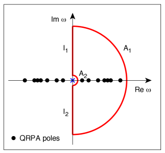
Figure 1: (Color online) The contour $D$ (oriented counterclockwise) in the complex-$\omega$ plane used to evaluate sum rules. The contour consists of two semicircles $A_{1}$ and $A_{2}$ (of radii $R_{A_{1}}$ and $R_{A_{2}}$, respectively) and two segments $I_{1}$ and $I_{2}$ on the imaginary axis. The positive QRPA poles are all located between $R_{A_{2}}$ and $R_{A_{1}}$.

In summary, regardless of the moment $k$, the sum rule is given by the integration along $D$:

$$m_{k}(\hat{F})=\frac{1}{2\pi i}\oint_{D}\omega^{k}S(\hat{F},\omega)d\omega=\sum_{\nu>0}\Omega_{\nu}^{k}|\langle\nu|\hat{F}|0\rangle|^{2}.$$ (17)

However, for certain moments $k$, some parts of path $D$ do not contribute to the sum rule. For odd values of $k$, the contributions from $I_{1}$ and $I_{2}$ cancel each other. Furthermore, for negative $k$, application of Jordan’s lemma, together with a limit of $R_{A_{1}}\to\infty$, allows for the removal of the contribution from $A_{1}$. For positive $k$, there is no pole at $\omega=0$, and the limit $R_{A_{2}}\to 0$ can be taken. Table 1 lists the portions of the contour $D$ required for each $k$. Furthermore, for even $k$, the contributions from $I_{1}$ and $I_{2}$ are identical. Similar contours were considered in Ref. Malov et al. (1977) to compute energy-weighted sum rules.

Table 1: Portions of the contour $D$ required for computing various sum rules $m_{k}$. For sum rules with even $k$, the contributions from $I_{1}$ and $I_{2}$ are identical.

$k$	Required portions of $D$
negative, even	$A_{2}$, $I_{1}$, $I_{2}$ ($R_{A_{1}}\to\infty$)
negative, odd	$A_{2}$ ($R_{A_{1}}\to\infty$)
0	$A_{1}$, $A_{2}$, $I_{1}$, $I_{2}$
positive, odd	$A_{1}$ ($R_{A_{2}}\to 0$)
positive, even	$A_{1}$, $I_{1}$, $I_{2}$ ($R_{A_{2}}\to 0$)

IV Results

IV.1 Numerical checks and benchmarking against MQRPA

To check the FAM approach to sum rules, following Refs. Stoitsov et al. (2011); Hinohara et al. (2013) we consider the oblate configuration of ²⁴Mg computed with the SLy4 Chabanat et al. (1998) Skyrme EDF. The HFB calculations were carried out with the DFT solver HFBTHO Stoitsov et al. (2013) in a model space of five harmonic oscillator shells by employing a volume pairing with the strength of $V_{0}=-125.20\,{\rm MeV\,fm}^{3}$ and a 60 MeV quasiparticle energy cutoff. The resulting oblate minimum of ²⁴Mg has nonzero pairing in protons and neutrons. The small single-particle model space employed makes it possible to benchmark FAM results against the matrix formulation of QRPA (MQRPA) Losa et al. (2010) without any further truncation. To compute spatial integrals we used Gauss-Hermite ($N_{\rm GH}=30$), Gauss-Laguerre ($N_{\rm GL}=30$), and Gauss-Legendre ($N_{\rm Leg}=30$) quadratures. The finite-amplitude expansion parameter $\eta$ was set to be $10^{-7}$, and the convergence criterion of the FAM was set such that the change of the individual FAM amplitudes from the previous iteration should be less than $10^{-5}$. The integration along semicircles $A_{1}$ and $A_{2}$ was discretized with $N_{A_{1}}$ and $N_{A_{2}}$ points, respectively. In addition, the integration along $I_{1}$ was discretized with $N_{I_{1}}$ points and evaluated using the composite Simpson’s rule. As for negative-$k$ moments, the composite Simpson’s rule was applied to the variable $1/\omega$ to describe the divergent behavior of integrand around $\omega=0$. In this particular test case, the smallest and largest energy MQRPA poles appear at 1.3 MeV and 128.7 MeV, respectively. Consequently, the contour radii were set to $R_{A_{2}}=1$ MeV and $R_{A_{1}}=200$ MeV. In order to systematically assess our numerical procedure for different moments $k$, we used the same contour $D$ for all cases, without simplifications listed in Table 1.

As far as the external field $\hat{F}$ is concerned, we considered the isoscalar (IS) and isovector (IV) monopole (M) and quadrupole (Q) operators:

$$\hat{F}^{\rm ISM}= \frac{eZ}{A}\sum_{i=1}^{A}r^{2}_{i}\,,$$ (18)

$$\hat{F}^{\rm IVM}= \sum_{i=1}^{A}e_{\rm eff}(\tau_{3i})r^{2}_{i}\hat{\tau}_{3i},$$ (19)

$$\hat{F}^{\rm ISQ}= \frac{eZ}{A}\sum_{i=1}^{A}r^{2}_{i}Y_{20}(\theta_{i},\varphi_{i})\,,$$ (20)

$$\hat{F}^{\rm IVQ}= \sum_{i=1}^{A}e_{\rm eff}(\tau_{3i})r^{2}_{i}Y_{20}(\theta_{i},\varphi_{i})\hat{\tau}_{3i},$$ (21)

where $e_{\rm eff}({\rm n})=eZ/A$ and $e_{\rm eff}({\rm p})=-eN/A$.

It is worth noting that neutron and proton pairing-rotational spurious modes, associated with the breaking of the particle number symmetry, are present in the $K^{\pi}=0^{+}$ sector. Fortunately, these modes – generated by the neutron and proton particle number operators – cannot be excited by particle-hole operators (18)-(21). Therefore, the presence of pairing-rotational spurious modes does not cause any additional difficulties Nakatsukasa et al. (2007); Stoitsov et al. (2011).

Table 2: The real part of the integral (17) for $-4\leq k\leq 4$ and $\hat{F}^{\rm ISM}$ (in ${\rm MeV}^{k}\,{\rm e}^{2}\,{\rm fm}^{4}$) along semicircle $A_{1}$ with $R_{A_{1}}=200$ MeV. The integral was discretized with $N_{A_{1}}$ points. The numbers in parentheses denote powers of 10.

$N_{A_{1}}$	$k=-4$	$k=-3$	$k=-2$	$k=-1$	$k=0$	$k=1$	$k=2$	$k=3$	$k=4$
2	-9.0(-9)	-2.6(-6)	-3.8(-4)	-2.7(-3)	14.4510	4195.31	608575	4318446	-23121542422
3	9.0(-9)	6.8(-8)	-1.7(-4)	1.1(-4)	13.8328	4199.78	574147	4338677	-10598058261
4	3.3(-9)	-2.6(-9)	-1.4(-4)	-5.7(-6)	13.5751	4199.39	562629	4336463	-8502934038
5	2.5(-9)	2.2(-10)	-1.3(-4)	4.1(-6)	13.4599	4199.44	557421	4336545	-7722808528
7	2.0(-9)	7.1(-12)	-1.2(-4)	2.9(-6)	13.3593	4199.44	552937	4336634	-7119788306
9	1.9(-9)	2.1(-12)	-1.1(-4)	2.9(-6)	13.3181	4199.44	551106	4336643	-6889795483
10	1.8(-9)	1.9(-12)	-1.1(-4)	2.9(-6)	13.3061	4199.44	550575	4336644	-6824728295
11	1.8(-9)	1.9(-12)	-1.1(-4)	2.9(-6)	13.2972	4199.44	550183	4336638	-6777106568
12	1.8(-9)	2.0(-12)	-1.1(-4)	2.9(-6)	13.2905	4199.44	549885	4336648	-6741178415
101	1.6(-9)	1.9(-12)	-1.1(-4)	2.9(-6)	13.2556	4199.44	548341	4336643	-6558793102
201	1.6(-9)	1.9(-12)	-1.1(-4)	2.9(-6)	13.2552	4199.44	548325	4336643	-6556876296
301	1.6(-9)	2.0(-12)	-1.1(-4)	2.9(-6)	13.2551	4199.44	548322	4336644	-6556517206

To begin with, we checked the convergence of the integral (17) along $A_{1}$, $A_{2}$, and $I_{1}$ with respect of the number of integration points. The results are presented in Tables 2-4 for the isoscalar monopole operator. As seen in Table 2, the integrals along $A_{1}$ are small for negative $k$. Analytically, these values should be zero for negative-odd values of $k$; hence, nonzero values in Table 2 reflect the numerical error of calculations. As far as the positive $k$ moments are concerned, the convergence is faster for odd-$k$ sum rules. In particular, the convergence for $k=1$ is excellent, since a 6-digit accuracy is achieved already with $N_{A_{1}}=5$. The integration along $A_{1}$ captures the total $m_{1}$ and $m_{3}$ sum rules; the result in Table 2 indicates that these sum rules can be computed very efficiently. Moreover, since the semicircle $A_{1}$ is located very far from the QRPA poles, FAM calculations along $A_{1}$ converge very quickly, typically after 6 iterations. Furthermore, each FAM calculation at a given $\omega$ along the contour is easily parallelizable; this could significantly reduce the total computational time, although not so many points are required for the convergence of $m_{1}$ and $m_{3}$.

Table 3: Similar to Table 2 but for the integration along $A_{2}$ for several values of $N_{A_{2}}$ with $R_{A_{2}}=1.0\,{\rm MeV}$.

$N_{A_{2}}$	$k=-4$	$k=-3$	$k=-2$	$k=-1$	$k=0$	$k=1$	$k=2$	$k=3$	$k=4$
5	-1.20929	0.0372710	3.26165	5.00438	3.23108	1.0(-3)	-1.22915	2.2(-3)	0.996926
11	-1.06784	0.0369978	3.21892	5.00387	3.18902	2.7(-5)	-1.09039	4.1(-5)	0.691152
15	-1.05236	0.0369925	3.21386	5.00386	3.18407	7.1(-6)	-1.07507	3.9(-6)	0.663895
16	-1.05021	0.0369910	3.21315	5.00385	3.18338	4.1(-6)	-1.07293	-7.8(-7)	0.660178
21	-1.04368	0.0369929	3.21099	5.00385	3.18127	6.2(-6)	-1.06646	-6.4(-7)	0.649056
31	-1.03883	0.0369918	3.20937	5.00385	3.17968	6.1(-6)	-1.06164	9.9(-7)	0.640898
51	-1.03625	0.0369916	3.20851	5.00385	3.17884	5.6(-6)	-1.05908	1.0(-6)	0.636594
101	-1.03512	0.0369918	3.20813	5.00385	3.17847	5.9(-6)	-1.05797	7.2(-7)	0.634728

Table 4: Similar to Table 2 but for the integration along $I_{1}$ for several values of $N_{I_{1}}$ with $R_{A_{1}}=200\,{\rm MeV}$ and $R_{A_{2}}=1.0\,{\rm MeV}$.

$N_{I_{1}}$	$k=-4$	$k=-3$	$k=-2$	$k=-1$	$k=0$	$k=1$	$k=2$	$k=3$	$k=4$
10	0.523854	-6.6(-8)	-1.472654	1.3(-7)	61.4767	-2.0(-6)	-208884	2.3(-2)	3356473886
30	0.523849	1.2(-6)	-1.478626	-1.6(-6)	61.7093	-6.0(-7)	-208523	-4.2(-3)	3356786248
50	0.523850	-1.1(-6)	-1.477671	1.4(-6)	61.7024	-2.2(-6)	-208522	3.3(-2)	3356787504
100	0.523850	-1.5(-6)	-1.477427	2.0(-6)	61.7044	-1.4(-6)	-208522	2.8(-2)	3356787251
200	0.523850	-8.7(-7)	-1.477417	1.2(-6)	61.7052	-1.8(-6)	-208522	2.2(-2)	3356787739

Table 3 shows the convergence of the integral (17) along $A_{2}$. This portion of the contour is required for the sum rules with negative $k$. Of most practical importance is the inverse energy-weighted sum rule $m_{-1}$. The value of $m_{-1}$ converges here with $N_{A_{2}}=16$ points. In general, as compared to integration along $A_{1}$, more FAM iterations are required to achieve reasonable convergence along $A_{2}$. In the case considered, typically 50 FAM iterations are necessary for each $\omega$. When choosing $R_{A_{2}}$ one has to keep in mind that its value should be smaller than the lowest QRPA pole, whose energy is not a priori known. At the same time, the convergence of FAM calculations for negative-$k$ moments deteriorates rapidly when $R_{A_{2}}$ gets too close to zero.

Table 4 illustrates the convergence along the segment $I_{1}$ on the imaginary axis. As discussed, this integration should be nonzero only for even-$k$ moments. The convergence for $k=0$ is reached rather slowly, especially when compared with the $k=4$ and $-4$ cases. This is because the Simpson’s formula used approximates the integrand with quadratic functions, which is a poor ansatz for $k=0$.

Table 5: Sum rules (in ${\rm MeV}^{k}\,{\rm e}^{2}\,{\rm fm}^{4}$) for the isoscalar and isovector monopole operators calculated with MQRPA and FAM. The FAM calculations were performed by using $N_{A_{1}}=301$, $N_{A_{2}}=101$, and $N_{I_{1}}=200$ integration points.

	$k=-4$	$k=-3$	$k=-2$	$k=-1$	$k=0$	$k=1$	$k=2$	$k=3$	$k=4$
MQRPA(ISM)	0.013077	0.037185	0.253118	5.00072	139.825	4200.82	131368	4342358	157906069
FAM(ISM)	0.012579	0.036992	0.253186	5.00385	139.844	4199.44	131277	4336644	157058272
MQRPA(IVM)	0.00063616	0.00273872	0.07120949	2.78540	113.908	4735.03	199525	8527358	370625216
FAM(IVM)	0.00043157	0.00275227	0.07133510	2.78615	113.908	4734.30	199510	8524830	368643941

To benchmark our FAM approach, in Table 5 we display the values of sum rules for the isoscalar and isovector monopole operators; they are compared with the MQRPA results based on the direct evaluation of the r.h.s. of Eq. (17). Overall, there is an excellent agreement between the two sets of calculations. This result indicates that the proposed FAM technique can be used to predict sum rules of interest in model spaces that are too large to be treated with MQRPA. The convergence of integration along $A_{2}$ is not sufficient in the case of $k=-4$; this sum rule is, however, less important than other moments discussed.

IV.2 Thouless theorem for energy-weighted sum rule

The Thouless theorem Thouless (1961) gives the relation between the energy-weighted sum rule $m_{1}(\hat{F})$ for isoscalar $\hat{F}=\sum_{i=1}^{A}f(\hat{\bm{r}}_{i})$ or isovector $\hat{F}=\sum_{i=1}^{A}f(\hat{\bm{r}}_{i})\hat{\tau}_{3i}$ one-body operators and the expectation value of the double commutator at the ground state Bertsch and Tsai (1975); Lipparini and Stringari (1989); Bohigas et al. (1979); Yannouleas (1987):

$$m_{1}(\hat{F})= \frac{1}{2}\langle[\hat{F},[\hat{H},\hat{F}]]\rangle=\frac{1}{2}(1+\kappa)\langle[\hat{F},[\hat{T},\hat{F}]]\rangle$$

$$= \displaystyle(1+\kappa)\frac{\hbar^{2}}{2m}\int|\nabla f(\bm{r})|^{2}\rho(\bm{r})d\bm{r}\,,$$ (22)

where $\hat{T}$ is the kinetic energy operator and $\kappa$ is the enhancement factor, which is present in the case when $\hat{F}$ is an isovector operator. The explicit expressions for the r.h.s. of Eq. (22) for the operators (18)-(21) are given in Appendix A.

The theorem is exact when both the ground state and the excited states are many-body shell-model states, and has been proven for HF+RPA Thouless (1961), HFB+QRPA Khan et al. (2002), and second RPA Papakonstantinou (2014). In the case of HF+RPA, expression (22) also holds for the Skyrme force due to the $\delta$-character of the momentum-dependent terms Brink and Leonardi (1976); Bohigas et al. (1979). However, as pointed out in Ref. Pastore et al. (2012), the theorem has not been proven for a generalized EDF, which is not explicitly related to an effective interaction. Deviations from relation (22) can be caused by, e.g., different assumptions about particle-hole and pairing channels, the Slater approximation to the Coulomb exchange term, approximations to spin-orbit and tensor terms Satuła and Dobaczewski (2014), and generalized density dependence Raimondi et al. (2011); Dobaczewski et al. (2012); Sadoudi et al. (2013). To the best of our knowledge, the Thouless theorem has not been proven in the case of generalized EDFs.

Table 6: The energy weighted $K^{\pi}=0^{+}$ sum rule (in ${\rm MeV\,e}^{2}\,{\rm fm}^{4}$) for the operators (18)-(21) at the oblate minimum of ²⁴Mg as a function of $N_{\rm sh}$. The FAM values were obtained by taking $R_{A_{1}}=200$ MeV and $N_{A_{1}}=12$; they are compared to HFB values (22). The results without time-odd terms except for the current-current coupling ($C_{t}^{j}\neq 0$ and $C_{t}^{s}(\rho_{0})=C_{t}^{\Delta s}=C_{t}^{\nabla j}=C^{T}_{t}=0$) $(a)$, and with the full time-odd functional except for the current-current and kinetic spin-spin couplings ($C_{t}^{j}=C^{T}_{t}=0,C_{t}^{s}(\rho_{0})\neq 0,C_{t}^{\Delta s}\neq 0$, and $C_{t}^{\nabla j}\neq 0$) $(b)$, obtained with $N_{\rm sh}$=20, are also listed.

$N_{\rm sh}$	FAM(ISM)	HFB(ISM)	FAM(IVM)	HFB(IVM)	FAM(ISQ)	HFB(ISQ)	FAM(IVQ)	HFB(IVQ)
5	4199.44	4303.67	4734.25	4752.37	762.638	767.933	848.110	845.235
10	4524.39	4502.75	4970.34	4940.08	779.019	775.724	852.995	849.015
15	4521.39	4523.80	4958.02	4960.52	776.587	776.161	849.482	849.116
20	4530.01	4529.46	4966.98	4966.01	777.425	776.832	850.145	849.747
20(a)	4530.07	-	4966.98	-	777.506	-	850.132	-
20(b)	5297.64	-	5298.46	-	905.461	-	905.441	-

In the following, we refer to the value (22) as the “HFB value” of the energy-weighted sum rule. In Table 6 the energy-weighted sum rules obtained in HFB and FAM are compared for different model spaces given by $N_{\rm sh}$. In a small model space of $N_{\rm sh}=5$, the difference between FAM and HFB values is non-negligible but quickly becomes small with $N_{\rm sh}$. This can be attributed to a poor representation of the operator $\hat{F}$ in small basis spaces, resulting in an error on the derivative of the function $f(\hat{\bm{r}})$ in Eq. (22). In spite of the fact that the SLy4 EDF combined with volume pairing cannot be related to a force, the numerical test in Table 6 demonstrates that the Thouless theorem provides a reasonably good approximation to the value of the sum rule $m_{1}$ for the Skyrme EDF.

In the notation of Ref. Dobaczewski and Dudek (1995), the time-odd part of the Skyrme EDF reads:

$${\cal E}_{\rm odd}= \sum_{t=0,1}\big{[}C^{s}_{t}(\rho_{0})\bm{s}^{2}_{t}+C^{\Delta s}_{t}\bm{s}_{t}\cdot\Delta\bm{s}_{t}$$

$$+C^{j}_{t}\bm{j}^{2}_{t}+C^{\nabla j}_{t}\bm{s}_{t}\cdot(\nabla\times\bm{j}_{t})+C^{T}_{t}\bm{s}_{t}\cdot\bm{T}_{t}\big{]}\,.$$ (23)

By taking the Skyrme interaction as a starting point, the time-odd and time-even coupling constants of the Skyrme EDF are related to each other. That is, by fixing time-even coupling constants, the time-odd part becomes also determined. This choice also guarantees the EDF’s gauge invariance Perlińska et al. (2004). In the EDF picture, however, the time-odd coupling constants could be treated as independent parameters, where some of them can be constrained by local gauge invariance Bender et al. (2002); Dobaczewski and Dudek (1995). With local gauge invariance assumed and tensor terms excluded, the last term of Eq. (IV.2), proportional to $C^{T}_{t}$, vanishes. In standard HFB calculations for even-even nuclei, the time-odd fields do not contribute because of time-reversal symmetry; hence, the time-odd part (IV.2) does not affect the HFB value (22). However, when time-reversal symmetry becomes broken, as in the case of FAM calculations, time-odd terms become active.

As shown in Table 6, the inclusion of the current-current term $C^{j}_{t}\bm{j}_{t}^{2}$ is necessary in the FAM to recover the HFB value of the energy-weighted sum rule of the monopole and quadrupole operators. This indicates that the gauge invariance of the term $\rho\tau-\bm{j}^{2}$ should not be broken when applying the Thouless theorem to QRPA sum rules. Other terms in the time-odd functional do not impact the energy-weighed sum rule. Local gauge invariance also couples the $C_{t}^{\nabla j}$ and $C_{t}^{\nabla J}$ terms, but the numerical results demonstrate that these do not affect the energy-weighted sum rule.

IV.3 Dielectric theorem for the inverse energy-weighted sum rule

The dielectric theorem connects the inverse-energy-weighted sum rule (related to nuclear polarizability) with the constrained potential energy surface. This theorem was proposed in Refs. Marshalek and da Providência (1973); Bohigas et al. (1979) for the HF case, and has been proven in the HFB framework in Ref. Capelli et al. (2009). Based on this theorem, the inverse energy-weighted sum rule $m_{-1}$ can be obtained from the curvature of the total energy ${\cal E}$ at equilibrium:

$$m_{-1}(\hat{F})= \frac{1}{2}\left.\frac{\partial^{2}}{\partial\lambda^{2}}{\cal E}(\lambda)\right|_{\lambda=0}$$

$$= \left.\frac{1}{2}\frac{\partial\left\langle\phi(\lambda)\right|\hat{F}\left|\phi(\lambda)\right\rangle}{\partial\lambda}\right|_{\lambda=0},$$ (24)

where the constrained HFB state $\left|\phi(\lambda)\right\rangle$ is obtained by minimizing the total Routhian containing a linear constraint $-\lambda\hat{F}$. We use the relation (IV.3) to compute the $m_{-1}$ sum rule. The derivative is evaluated with a finite difference of $\Delta\lambda\,=\,0.0001\,{\rm MeV\,e}^{-1}\,{\rm fm}^{-2}$. The resulting $m_{-1}$ values are compared with those from the FAM in Table 7. A good agreement is found already in a small model space ($N_{\rm sh}=5$) where $m_{-1}$ is not fully converged, indicating that the dielectric theorem works well, independently of the size of the model space. This finding is consistent with the proof of Ref. Capelli et al. (2009), which applies to an arbitrary size of quasiparticle space.

Table 7: Inverse energy-weighted sum rule (in ${\rm MeV}^{-1}\,{\rm e}^{2}\,{\rm fm}^{4}$) computed using the dielectric theorem (HFB) and the FAM for various sizes of the model space given by $N_{\rm sh}$. FAM calculations were performed using $N_{A_{2}}=22$ and $R_{A_{2}}=1.0$ MeV.

$N_{\rm sh}$	FAM(ISM)	HFB(ISM)	FAM(IVM)	HFB(IVM)	FAM(ISQ)	HFB(ISQ)	FAM(IVQ)	HFB(IVQ)
5	5.00385	5.00375	2.78615	2.78614	4.44830	4.44765	0.798680	0.798680
10	11.2033	11.2102	5.09467	5.09671	5.21547	5.21586	1.07516	1.07524
15	12.4930	12.5009	5.71677	5.71960	5.31250	5.31268	1.12916	1.12910
20	12.9506	12.9634	6.06842	6.07304	5.35499	5.35730	1.15744	1.15771

IV.4 Example of systematic calculations

Table 8: Isoscalar monopole and quadrupole energy-weighted $K^{\pi}=0^{+}$ sum rules in units of ${\rm MeV\,e}^{2}\,{\rm fm}^{4}$ computed with the FAM and the HFB techniques for ^142-152Nd and ^144-154Sm isotopes. The quadrupole deformation $\beta$, neutron and proton pairing gaps ($\Delta_{\rm n}$ and $\Delta_{\rm p}$, respectively), and total rms radius $\sqrt{\langle r^{2}\rangle}$ are also shown.

	$\beta$	$\Delta_{\rm n}$(MeV)	$\Delta_{\rm p}$(MeV)	$\sqrt{\langle r^{2}\rangle}$(fm)	HFB(ISM)	FAM(ISM)	HFB(ISQ)	FAM(ISQ)
142Nd	0.0	0.00	1.21	4.92	50497	50724	10046	10068
144Nd	0.09	0.49	1.09	4.95	50453	50647	10606	10626
146Nd	0.15	0.55	1.00	4.99	50590	50769	11042	11062
148Nd	0.21	0.00	0.93	5.03	50788	50936	11412	11429
150Nd	0.31	0.64	0.00	5.11	51667	51806	12287	12301
152Nd	0.32	0.00	0.00	5.14	51649	51762	12375	12383
144Sm	0.0	0.00	1.10	4.94	53635	53873	10670	10693
146Sm	0.06	0.55	1.08	4.97	53492	53712	11048	11069
148Sm	0.16	0.56	1.07	5.01	53754	53957	11770	11792
150Sm	0.21	0.16	0.93	5.06	53979	54145	12189	12207
152Sm	0.28	0.57	0.69	5.11	54474	54646	12768	12786
154Sm	0.32	0.09	0.65	5.16	54707	54849	13071	13084

As an illustrative example, we discuss the energy-weighted $K^{\pi}=0^{+}$ sum rules in the shape transitional region of ^142-152Nd and ^144-154Sm. The calculations were carried out by using the SLy4 EDF parameterization with a volume pairing strength $V_{\rm n}=V_{\rm p}=-190\,{\rm MeV\,fm}^{3}$ in the model space of $N_{\rm sh}=20$ oscillator shells. The pairing strength was adjusted to reproduce the experimental proton pairing gap of 1.23 MeV in ¹⁴²Nd. In this realistic calculation we use $N_{\rm GH}=N_{\rm GL}=40$ and $N_{\rm Leg}=80$, which are the recommended values based on recent analysis Stoitsov et al. (2013). The FAM contour integration was carried out using a semicircle with $R_{A_{1}}=200$ MeV, discretized with $N_{A1}=12$ points.

Table 8 summarizes the results. The calculated ground state properties show a gradual spherical-to-deformed shape transition with increasing neutron number. Moreover, in some of the isotopes we predict pairing collapse. For that reason, the chosen set of nuclei is representative of a realistic situation encountered in global surveys across the nuclear landscape, where deformations and pairing may vary rapidly as a function of proton and neutron number.

The energy-weighted sum rules computed with the FAM agree well with the HFB expressions of Appendix A. This agreement holds regardless of nuclear shape or pairing. As expected, the energy-weighted sum rule for the isoscalar monopole operator increases with $N$ in the region of the shape transition; this is attributed to an increase of the root mean square radius with deformation. Similarly, the isoscalar quadrupole operator increases even more rapidly with increasing quadrupole deformation.

Next, we consider the energy weighted sum rules in constrained HFB states. The constrained HFB potential energy curve as a function of quadrupole moment was obtained using the quadratic constraint. The contribution from the quadratic constraining potential was included consistently to the residual field in the FAM. This kind of calculation represents local QRPA on top of constrained HFB Hinohara et al. (2010); it contains dynamical information about non-equilibrium configurations in the deformation space.

The energy-weighted sum rule of the isoscalar quadrupole operator as a function of quadrupole deformation is shown in Fig. 2. The sum rule increases monotonically with $\beta$ and agrees very well with HFB values. This, together with results presented in Table 8, indicates that the Thouless theorem provides a good approximation to the energy weighted sum rule within the Skyrme-EDF picture, which is not based on the underlying Hamiltonian.

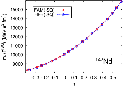
Figure 2: (Color online) Energy-weighted sum rule of the isoscalar quadrupole operator in ¹⁴²Nd obtained in the HFB (solid line with asterisks) and FAM (dashed line with open circles) frameworks as a function of quadrupole deformation $\beta$ for the constrained HFB solutions.

In passing, we should note that when departing from the HFB minimum, there is a possibility of imaginary energy QRPA solutions; in such cases, a pair of QRPA poles would appear on the imaginary axis. Although one expects no contribution to odd-$k$ sum rules from such a pair, a careful consideration needs to be given to the choice of integration contour in the FAM. A general extension of the complex FAM formalism to the case of local QRPA will be an interesting avenue for future studies.

V Conclusions

We propose an efficient formalism to compute sum rules by using the contour integration formalism within the complex-energy finite-amplitude method. In particular when the order of the moment is odd, the obtained expression becomes extremely simple, as the sum rules appear as expansion coefficients of the Laurent series of the response function. The new formalism has been successfully benchmarked against the matrix diagonalization method of QRPA.

We compare the energy-weighted sum rule obtained in the FAM with those based on the Thouless theorem. Although the double commutator cannot be evaluated for general energy density functionals that are not based on a Hamiltonian, the numerical results indicate that the theorem provides a very good approximation to $m_{1}$ when a large model space is employed and local gauge symmetry of the EDF is satisfied. The inverse-energy-weighted sum rule was compared with the constrained HFB result using the dielectric theorem, and a perfect agreement was obtained regardless of the model space.

Our results suggest that sum rules can be computed efficiently in the FAM even in cases when other methods are not easily available (e.g., the Thouless theorem cannot be applied or constrained calculations cannot be carried out because of self-consistent symmetries assumed). The extension of the formalism to non-Hermitian operators is also straightforward, as it has already been applied to the beta-decay rates with pn-FAM Mustonen et al. (2014).

The FAM approach to sum rules promises to add new functionality to the EDF optimization framework of Refs. Kortelainen et al. (2010, 2012, 2014) as it will allow adding new kinds of data on multipole- and charge-exchange strength to the set of fit-observables defining the objective function. The new FAM technique can be very useful when studying the nuclear response to non-trivial operators such as the nuclear Schiff moment, which is closely related to the isoscalar dipole operator Jesus and Engel (2005); Auerbach et al. (2014).

Appendix A Thouless theorem for monopole and quadrupole operators

According to the Thouless theorem (22), the energy-weighted sum rule for isoscalar monopole and quadrupole operators of an axially-deformed nucleus are:

$$m_{1}({\rm ISM})= 4e^{2}\left(\frac{Z}{A}\right)^{2}\frac{\hbar^{2}}{2m}A\langle r^{2}\rangle\,,$$ (25)

$$m_{1}({\rm ISQ})= e^{2}\left(\frac{Z}{A}\right)^{2}\frac{\hbar^{2}}{2m}\frac{5}{2\pi}A\langle r^{2}\rangle\left(1+\sqrt{\frac{5}{4\pi}}\beta\right)\,.$$ (26)

where $\langle r^{2}\rangle$ is the total rms squared radius and $\beta$ is the mass quadrupole deformation parameter:

$$\beta= \sqrt{\frac{\pi}{5}}\frac{1}{A\langle r^{2}\rangle}\int(3z^{2}-r^{2})\rho(\bm{r})d\bm{r}.$$ (27)

For isovector operators, there appears an enhancement factor

$$\kappa=\frac{8m}{\hbar^{2}}(C^{\tau}_{0}-C^{\tau}_{1})\frac{\displaystyle\int|\nabla f(\bm{r})|^{2}\rho_{\rm n}(\bm{r})\rho_{\rm p}(\bm{r})d\bm{r}}{\displaystyle\int|\nabla f(\bm{r})|^{2}\rho(\bm{r})d\bm{r}},$$ (28)

where – in the notation of Ref. Dobaczewski and Dudek (1995) – $C^{\tau}_{t}$ is the coupling constant of the term $\rho_{t}\tau_{t}$ in the EDF. The expressions for the isovector monopole and quadrupole operators are:

$$m_{1}({\rm IVM})= 4e^{2}\frac{\hbar^{2}}{2m}\frac{NZ}{A^{2}}\left[Z\langle r^{2}\rangle_{\rm n}+N\langle r^{2}\rangle_{\rm p}\right](1+\kappa_{\rm IVM}),$$ (29)

$$\kappa_{\rm IVM}= \frac{8m}{\hbar^{2}}(C^{\tau}_{0}-C^{\tau}_{1})\frac{1}{A\langle r^{2}\rangle}\int r^{2}\rho_{\rm n}(\bm{r})\rho_{\rm p}(\bm{r})d\bm{r},$$ (30)

and

$$m_{1}({\rm IVQ})= e^{2}\frac{\hbar^{2}}{2m}\frac{NZ}{A^{2}}\frac{5}{2\pi}\left[Z\langle r^{2}\rangle_{\rm n}\left(1+\sqrt{\frac{5}{4\pi}}\beta_{\rm n}\right)\right.$$

$$+ \left.N\langle r^{2}\rangle_{\rm p}\left(1+\sqrt{\frac{5}{4\pi}}\beta_{\rm p}\right)\right](1+\kappa_{\rm IVQ}),$$ (31)

$$\kappa_{\rm IVQ}= \frac{8m}{\hbar^{2}}(C^{\tau}_{0}-C^{\tau}_{1})\frac{1}{\displaystyle 2A\langle r^{2}\rangle\left(1+\sqrt{\frac{5}{4\pi}}\beta\right)}$$

$$\times \int(3z^{2}+r^{2})\rho_{\rm n}(\bm{r})\rho_{\rm p}(\bm{r})d\bm{r},$$ (32)

where subscripts n/p indicate neutron/proton expectation values respectively.

References

- Bohr and Mottelson (1998) A. Bohr and B. R. Mottelson, Nuclear structure, Vol. 2: Nuclear deformations (World Scientific Pub. Co., Singapore, 1998).
- Ring and Schuck (2000) P. Ring and P. Schuck, The Nuclear Many-Body Problem (Springer-Verlag, 2000).
- Harakeh and van der Woude (2001) M. N. Harakeh and A. van der Woude, Giant Resonances: Fundamental High-Frequency Modes of Nuclear Excitation (Oxford University Press, 2001).
- Bender et al. (2003) M. Bender, P.-H. Heenen, and P.-G. Reinhard, Rev. Mod. Phys. 75, 121 (2003).
- Klüpfel et al. (2009) P. Klüpfel, P.-G. Reinhard, T. Bürvenich, and J. Maruhn, Phys. Rev. C 79, 034310 (2009).
- Kortelainen et al. (2010) M. Kortelainen, T. Lesinski, J. Moré, W. Nazarewicz, J. Sarich, N. Schunck, M. V. Stoitsov, and S. Wild, Phys. Rev. C 82, 024313 (2010).
- Kortelainen et al. (2012) M. Kortelainen, J. McDonnell, W. Nazarewicz, P.-G. Reinhard, J. Sarich, N. Schunck, M. V. Stoitsov, and S. M. Wild, Phys. Rev. C 85, 024304 (2012).
- Kortelainen et al. (2014) M. Kortelainen, J. McDonnell, W. Nazarewicz, E. Olsen, P.-G. Reinhard, J. Sarich, N. Schunck, S. M. Wild, D. Davesne, J. Erler, and A. Pastore, Phys. Rev. C 89, 054314 (2014).
- Erler et al. (2013) J. Erler, C. Horowitz, W. Nazarewicz, M. Rafalski, and P.-G. Reinhard, Phys. Rev. C 87, 044320 (2013).
- Erler et al. (2012) J. Erler, N. Birge, M. Kortelainen, W. Nazarewicz, E. Olsen, A. M. Perhac, and M. Stoitsov, Nature 486, 509 (2012).
- Afanasjev et al. (2013) A. V. Afanasjev, S. E. Agbemava, D. Ray, and P. Ring, Phys. Lett. B 726, 680 (2013).
- Goriely and Capote (2014) S. Goriely and R. Capote, Phys. Rev. C 89, 054318 (2014).
- Giai and Sagawa (1981) N. V. Giai and H. Sagawa, Phys. Lett. B 106, 379 (1981).
- Friedrich and Reinhard (1986) J. Friedrich and P.-G. Reinhard, Phys. Rev. C 33, 335 (1986).
- Reinhard et al. (1999) P.-G. Reinhard, D. Dean, W. Nazarewicz, J. Dobaczewski, J. Maruhn, and M. Strayer, Phys. Rev. C 60, 014316 (1999).
- Agrawal et al. (2005) B. Agrawal, S. Shlomo, and V. Au, Phys. Rev. C 72, 014310 (2005).
- Trippa et al. (2008) L. Trippa, G. Colò, and E. Vigezzi, Phys. Rev. C 77, 061304 (2008).
- Dutra et al. (2012) M. Dutra, O. Lourenço, J. Sá Martins, A. Delfino, J. Stone, and P. Stevenson, Phys. Rev. C 85, 035201 (2012).
- Roca-Maza et al. (2012) X. Roca-Maza, G. Colò, and H. Sagawa, Phys. Rev. C 86, 031306 (2012).
- Marshalek and da Providência (1973) E. R. Marshalek and J. da Providência, Phys. Rev. C 7, 2281 (1973).
- Bertsch and Tsai (1975) G. Bertsch and S. Tsai, Phys. Rep. 18, 125 (1975).
- Lipparini and Stringari (1989) E. Lipparini and S. Stringari, Phys. Rep. 175, 103 (1989).
- Bohigas et al. (1979) O. Bohigas, A. M. Lane, and J. Martorell, Phys. Rep. 51, 267 (1979).
- Brink and Leonardi (1976) D. M. Brink and R. Leonardi, Nucl. Phys. A 258, 285 (1976).
- Gleissl et al. (1990) P. Gleissl, M. Brack, J. Meyer, and P. Quentin, Ann. Phys. 197, 205 (1990).
- Reinhard (1992) P.-G. Reinhard, Ann. Phys. (Berlin) 504, 632 (1992).
- Capelli et al. (2009) L. Capelli, G. Colò, and J. Li, Phys. Rev. C 79, 054329 (2009).
- Soubbotin et al. (2004) V. Soubbotin, V. Tselyaev, and X. Viñas, Phys. Rev. C 69, 064312 (2004).
- Reinhard and Nazarewicz (2010) P.-G. Reinhard and W. Nazarewicz, Phys. Rev. C 81, 051303 (2010).
- Piekarewicz et al. (2012) J. Piekarewicz, B. K. Agrawal, G. Colò, W. Nazarewicz, N. Paar, P.-G. Reinhard, X. Roca-Maza, and D. Vretenar, Phys. Rev. C 85, 041302 (2012).
- Reinhard and Nazarewicz (2013) P.-G. Reinhard and W. Nazarewicz, Phys. Rev. C 87, 014324 (2013).
- Stringari et al. (1976) S. Stringari, R. Leonardi, and D. Brink, Nucl. Phys. A 269, 87 (1976).
- Pastore et al. (2012) A. Pastore, D. Davesne, Y. Lallouet, M. Martini, K. Bennaceur, and J. Meyer, Phys. Rev. C 85, 054317 (2012).
- Chamel and Goriely (2010) N. Chamel and S. Goriely, Phys. Rev. C 82, 045804 (2010).
- Thouless (1961) D. J. Thouless, Nucl. Phys. 22, 78 (1961).
- Khan et al. (2002) E. Khan, N. Sandulescu, M. Grasso, and N. Van Giai, Phys. Rev. C 66, 024309 (2002).
- Centelles et al. (2005) M. Centelles, X. Viñas, S. K. Patra, J. N. De, and T. Sil, Phys. Rev. C 72, 014304 (2005).
- Matsuo (2001) M. Matsuo, Nucl. Phys. A 696, 371 (2001).
- Johnson et al. (1999) C. Johnson, G. Bertsch, and W. Hazelton, Comput. Phys. Comm. 120, 155 (1999).
- Nevo Dinur et al. (2014) N. Nevo Dinur, N. Barnea, C. Ji, and S. Bacca, Phys. Rev. C 89, 064317 (2014).
- Nakatsukasa et al. (2007) T. Nakatsukasa, T. Inakura, and K. Yabana, Phys. Rev. C 76, 024318 (2007).
- Avogadro and Nakatsukasa (2011) P. Avogadro and T. Nakatsukasa, Phys. Rev. C 84, 014314 (2011).
- Stoitsov et al. (2011) M. Stoitsov, M. Kortelainen, T. Nakatsukasa, C. Losa, and W. Nazarewicz, Phys. Rev. C 84, 041305 (2011).
- Mustonen et al. (2014) M. T. Mustonen, T. Shafer, Z. Zenginerler, and J. Engel, Phys. Rev. C 90, 024308 (2014).
- Pei et al. (2014) J. C. Pei, M. Kortelainen, Y. N. Zhang, and F. R. Xu, Phys. Rev. C 90, 051304 (2014).
- Liang et al. (2013) H. Liang, T. Nakatsukasa, Z. Niu, and J. Meng, Phys. Rev. C 87, 054310 (2013).
- Nikšić et al. (2013) T. Nikšić, N. Kralj, T. Tutiš, D. Vretenar, and P. Ring, Phys. Rev. C 88, 044327 (2013).
- Inakura et al. (2009) T. Inakura, T. Nakatsukasa, and K. Yabana, Phys. Rev. C 80, 044301 (2009).
- Inakura et al. (2011) T. Inakura, T. Nakatsukasa, and K. Yabana, Phys. Rev. C 84, 021302 (2011).
- Avogadro and Nakatsukasa (2013) P. Avogadro and T. Nakatsukasa, Phys. Rev. C 87, 014331 (2013).
- Hinohara et al. (2013) N. Hinohara, M. Kortelainen, and W. Nazarewicz, Phys. Rev. C 87, 064309 (2013).
- Malov et al. (1977) L. A. Malov, V. O. Nesterenko, and V. G. Solovèv, Teoret.. Mat. Fiz. 32, 134 (1977).
- Chabanat et al. (1998) E. Chabanat, P. Bonche, P. Haensel, J. Meyer, and R. Schaeffer, Nucl. Phys. A 635, 231 (1998).
- Stoitsov et al. (2013) M. V. Stoitsov, N. Schunck, M. Kortelainen, N. Michel, H. Nam, E. Olsen, J. Sarich, and S. Wild, Comp. Phys. Comm. 184, 1592 (2013).
- Losa et al. (2010) C. Losa, A. Pastore, T. Døssing, E. Vigezzi, and R. A. Broglia, Phys. Rev. C 81, 064307 (2010).
- Yannouleas (1987) C. Yannouleas, Phys. Rev. C 35, 1159 (1987).
- Papakonstantinou (2014) P. Papakonstantinou, Phys. Rev. C 90, 024305 (2014).
- Satuła and Dobaczewski (2014) W. Satuła and J. Dobaczewski, Phys. Rev. C 90, 054303 (2014).
- Raimondi et al. (2011) F. Raimondi, B. Carlsson, and J. Dobaczewski, Phys. Rev. C 83, 054311 (2011).
- Dobaczewski et al. (2012) J. Dobaczewski, K. Bennaceur, and F. Raimondi, J. Phys. G 39, 125103 (2012).
- Sadoudi et al. (2013) J. Sadoudi, M. Bender, K. Bennaceur, D. Davesne, R. Jodon, and T. Duguet, Phys. Scr. 2013, 014013 (2013).
- Dobaczewski and Dudek (1995) J. Dobaczewski and J. Dudek, Phys. Rev. C 52, 1827 (1995).
- Perlińska et al. (2004) E. Perlińska, S. G. Rohoziński, J. Dobaczewski, and W. Nazarewicz, Phys. Rev. C 69, 014316 (2004).
- Bender et al. (2002) M. Bender, J. Dobaczewski, J. Engel, and W. Nazarewicz, Phys. Rev. C 65, 054322 (2002).
- Hinohara et al. (2010) N. Hinohara, K. Sato, T. Nakatsukasa, M. Matsuo, and K. Matsuyanagi, Phys. Rev. C 82, 064313 (2010).
- Jesus and Engel (2005) J. H. d. Jesus and J. Engel, Phys. Rev. C 72, 045503 (2005).
- Auerbach et al. (2014) N. Auerbach, C. Stoyanov, M. R. Anders, and S. Shlomo, Phys. Rev. C 89, 014335 (2014).