Two-body state with $p$-wave interaction in one-dimensional waveguides under transversely anisotropic confinement

Abstract

We theoretically study two atoms with $p$-wave interaction in a one-dimensional waveguide, and investigate how the transverse anisotropy of the confinement affects the two-body state, especially, the properties of the resonance. For bound-state solution, we find there are totally three two-body bound states due to the richness of the orbital magnetic quantum number of $p$-wave interaction, while only one bound state is supported by $s$-wave interaction. Two of them become nondegenerate due to the breaking of the rotation symmetry under transversely anisotropic confinement. For scattering solution, the effective one-dimensional scattering amplitude and scattering length are derived. We find the position of the $p$-wave confinement-induced resonance shifts apparently as the transverse anisotropy increases. In addition, a two-channel mechanism for confinement-induced resonance in a one-dimensional waveguide is generalized to $p$-wave interaction, which was proposed only for $s$-wave interaction before. All our calculations are based on the parameterization of the ⁴⁰K atom experiments, and can be confirmed in future experiments.

I Introduction

Nowadays, the confinement-induced resonance (CIR) as one of the most intriguing phenomena in low-dimensional systems has attracted a great deal of interest. It was first predicted by Olshanii when considering the two-body $s$-wave scattering problem in quasi-one-dimensional (quasi-1D) waveguides Olshanii1998 . Subsequently, this study was extended to quasi-two-dimensional (quasi-2D) systems Petrov2000B ; Petrov2001I . In the past decade, an impressive amount of experimental and theoretical efforts have been devoted to confirm the existence of CIRs and explore the important consequences Bergeman2003A ; Granger2004T ; Moritz2005C ; Gunter2005P ; Pricoupenko2008R ; Haller2009R ; Haller2010C ; Peng2010C ; Zhang2011C ; Frohlich2011R ; Peng2011C ; Sala2012I ; Giannakeas2011R ; Peng2012T ; Peng2014M . To date, CIR has already become a fundamental technique in studying strongly interacting low-dimensional quantum gases.

The $p$-wave interaction is of particular interest, since it is the simplest high-partial-wave interaction with non-zero orbital angular momentum $l=1$. This leads to a spatial anisotropic scattering in few-body physics, and open a new method to manipulate resonant cold atomic interactions by using the magnetic field vector, as indicated in our previous work Peng2014M . For many-body physics, the high-partial-wave interaction may also result in physically abundant quantum phase transitions, which are absent in $s$-wave interaction Ohashi2005B ; Ho2005F ; Cheng2005A ; Iskin2006E . In addition, the $p$-wave scattering dominates the low-energy interaction between spin-polarized Fermi atoms (all in one hyperfine state) due to the Fermi-Dirac statistics, which provide an ideal candidate to study the $p$-wave scattering properties in cold atoms Zhang2004P ; Ticknor2004M .

For low-dimensional quantum systems, the external trap potential is one another freedom to manipulate two-body resonant interactions, and it is interesting to identify how CIR is affected when the external confinement changes. For example, in 1D Bose ¹³³Cs atoms with $s$-wave interaction, it is found that the transverse harmonic anisotropy shifts the position of CIR Peng2010C ; Zhang2011C , besides, CIR splits due to the anharmonicity of the transverse trap Haller2010C ; Peng2011C ; Sala2012I . Naturally, it is also important to investigate how the external confinement affects the low-dimensional resonant $p$-wave interaction between spin-polarized Fermi atoms, such as ⁴⁰K atoms.

In this paper, we study the influence of the transverse anisotropy on two-body state with $p$-wave interaction, especially, the scattering resonance in quasi-1D waveguides. We solve the two-body problem in a quasi-1D waveguide under transversely anisotropic confinement. The $p$-wave interaction is modeled by the contact pseudopotential including the effective range Peng2011H . This model neglects the spatial anisotropy of $p$-wave interaction , which is not the focus of this work. However, it is already sufficient enough to study how the external trap affects the $p$-wave CIR. Due to the non-zero orbital angular momentum, we find there are totally three bound states for $p$-wave interaction in the waveguide, while the $s$-wave pseudopotential supports only one two-body bound state. Two of them become nondegenerate as the transverse confinement changes from isotropic to anisotropic, which breaks the rotation symmetry around the waveguide. For scattering solution, we calculate the effective 1D scattering amplitude as well as the 1D scattering length, and predict the scattering resonance for any transverse anisotropy, whose position shows an apparent shift with increasing anisotropy. In addition, we present an effective two-channel mechanism for $p$-wave CIR, which was first proposed only for $s$-wave interaction Bergeman2003A . In this two-channel picture, the transverse ground state and the remaining transverse excited modes play roles of open and closed channels, respectively. When a bound state in the closed channel exists, and becomes energetically degenerate with the scattering threshold of the open channel, a scattering resonance is expected. All our calculations are based on the parameterization of the ⁴⁰K atom experiments Ticknor2004M ; Gunter2005P , and can be confirmed in future experiments.

In the following, we first study the properties of two-body bound states with $p$-wave interaction in a transversely anisotropic waveguide (Sec. II), and then present the scattering solution in Sec. III as well. We calculate the effective 1D scattering amplitude and 1D scattering length, and discuss how the transverse anisotropy of the confinement affects the $p$-wave CIR in details. In Sec. IV, a two-channel mechanism is presented for $p$-wave CIR. The main results are concluded in Sec. V.

II bound-state solutions

In order to simplify the problem, let us consider two atoms confined in a quasi-1D waveguide with a tight transverse harmonic potential (in $x-y$ plane). The transverse trap frequencies are $\omega_{x,y}$ , and the atoms can freely move along $z$ axis. The transverse anisotropy is characterized by $\eta=\omega_{x}/\omega_{y}$ . Unlike the $s$-wave interaction, the $p$-wave interaction is strongly energy-dependence due to the narrow-width property Ticknor2004M . Thus, one additional parameter named effective range should be included Peng2011H ; Yip2008E ; Suzuki2009T ; Idziaszek2009A . In harmonic traps, the center-of-mass (c.m.) motion is decoupled from the relative part, and we only need to solve the relative motion, while the c.m. motion is a simple harmonic oscillator. By dropping the c.m. motion off, the relative motion of two atoms is described by the following Hamiltonian,

$$\mathcal{H}=-\frac{\hbar^{2}}{2\mu}\frac{\partial^{2}}{\partial z^{2}}+\mathcal{H}_{\perp}+\mathcal{V}_{1},$$ (1)

where

$$\mathcal{H}_{\perp}=-\frac{\hbar^{2}}{2\mu}\left(\frac{\partial^{2}}{\partial x^{2}}+\frac{\partial^{2}}{\partial y^{2}}\right)+\frac{1}{2}\mu\omega^{2}\left(\eta^{2}x^{2}+y^{2}\right),$$ (2)

$\mu$ is the reduced mass, and $\omega$ is the trap frequency in $y$ aixs (we omit the subscript $y$ without ambiguity). The interatomic interaction $\mathcal{V}_{1}\left(\mathbf{r}\right)$ is modeled by the $p$-wave pseudopotential Peng2011H ,

$$\mathcal{V}_{1}\left(\mathbf{r}\right)=\frac{\pi\hbar^{2}}{\mu}\left(\frac{1}{v_{1}}-\frac{1}{2}r_{1}k^{2}\right)^{-1}\overleftarrow{\nabla}\delta\left(\mathbf{r}\right)\frac{\partial^{3}}{\partial r^{3}}r^{3}\overrightarrow{\nabla},$$ (3)

where $v_{1}$ and $r_{1}$ are the three-dimensional (3D) $p$-wave scattering volume and effective range (with a dimension of inverse length), respectively, which can be tuned by using $p$-wave Feshbach resonances Ticknor2004M ; Zhang2004P . $k$ is the relative wavenumber, related to the relative energy of two atoms as $E=\hbar^{2}k^{2}/\left(2\mu\right)$ . The symbol $\overleftarrow{\nabla}$ ($\overrightarrow{\nabla}$) denotes the gradient operator that acts to the left (right) of the pseudopotential.

For the bound-state problem, the wavefunction can formally be written as

$$\psi\left(\mathbf{r}\right)=-\int d^{3}\mathbf{r}^{\prime}G_{E}\left(\mathbf{r},\mathbf{r}^{\prime}\right)\mathcal{V}_{1}\left(\mathbf{r}^{\prime}\right)\psi\left(\mathbf{r}^{\prime}\right),$$ (4)

where $G_{E}\left(\mathbf{r},\mathbf{r}^{\prime}\right)$ is the single-particle Green’s function with energy $E$ , and satisfies

$$\left(-\frac{\hbar^{2}}{2\mu}\frac{\partial^{2}}{\partial z^{2}}+\mathcal{H}_{\perp}-E\right)G_{E}\left(\mathbf{r},\mathbf{r}^{\prime}\right)=\delta\left(\mathbf{r}-\mathbf{r}^{\prime}\right).$$ (5)

The Green’s function can be expanded in series of the eigen-states of non-interacting Hamiltonian as,

$$G_{E}\left(\mathbf{r},\mathbf{r}^{\prime}\right)=\sum_{n_{1}=0}^{\infty}\sum_{n_{2}=0}^{\infty}\int_{-\infty}^{\infty}dk_{z}\\ C_{n_{1}n_{2}}\left(k_{z}\right)\phi_{n_{1}}\left(\frac{\sqrt{\eta}x}{d}\right)\phi_{n_{2}}\left(\frac{y}{d}\right)\frac{e^{ik_{z}z}}{\sqrt{2\pi}},$$ (6)

where $\phi_{\nu}\left(\cdot\right)$ is the eigen-state of 1D harmonic oscillator, $d=\sqrt{\hbar/\mu\omega}$ is the harmonic length in $y$ aixs, and $k_{z}$ is the wavenumber along the waveguide ($z$ axis). Inserting Eq.(6) into Eq.(5) and using the completeness of the eigenstates of the non-interacting Hamiltonian, we may easily obtain the coefficients $C_{n_{1}n_{2}}\left(k_{z}\right)$ , and then after some straightforward algebra (the derivation is similar to Eq.(24) in Peng2010C ), the Green’s function takes the following integral representation,

$$G_{E}\left(\mathbf{r},\mathbf{r}^{\prime}\right)=\frac{1}{\pi^{3/2}d^{3}\hbar\omega}\int_{0}^{\infty}\frac{d\tau\,e^{\epsilon\tau}}{\sqrt{2\tau}}\exp\left[-\frac{\left(z-z^{\prime}\right)^{2}}{2d^{2}\tau}\right]\\ \times\frac{\sqrt{\eta}}{\sqrt{1-e^{-2\eta\tau}}}\exp\left[\eta\frac{2x^{\prime}x-\left(x^{\prime 2}+x^{2}\right)\cosh\left(\eta\tau\right)}{2d^{2}\sinh\left(\eta\tau\right)}\right]\\ \times\frac{1}{\sqrt{1-e^{-2\tau}}}\exp\left[\frac{2y^{\prime}y-\left(y^{\prime 2}+y^{2}\right)\cosh\tau}{2d^{2}\sinh\tau}\right],$$ (7)

which is valid for $\epsilon\equiv E/\hbar\omega-\left(\eta+1\right)/2<0$ . Combining Eqs.(3) and (4), the bound-state wavefunction takes the form

$$\psi\left(\mathbf{r}\right)=-\frac{\pi\hbar^{2}}{\mu}\left(\frac{1}{v_{1}}-\frac{1}{2}r_{1}k^{2}\right)^{-1}\\ \cdot\sum_{n}\mathcal{R}_{n}\left[\frac{\partial}{\partial r_{n}^{\prime}}G_{E}\left(\mathbf{r},\mathbf{r}^{\prime}\right)\right]_{r^{\prime}=0},$$ (8)

where the summation is over $n=x,y,z$ , and $r_{x}\equiv x,\,r_{y}\equiv y,\,r_{z}\equiv z$ . Here, we have defined the coefficent

$$\mathcal{R}_{n}\equiv\left[\frac{\partial^{3}}{\partial r^{3}}r^{3}\frac{\partial}{\partial r_{n}}\psi\left(\mathbf{r}\right)\right]_{r=0}.$$ (9)

Acting $\frac{\partial^{3}}{\partial r^{3}}r^{3}\frac{\partial}{\partial r_{n}}$ on both sides of Eq.(8) and setting $r=0$ , we obtain the following secular equation,

$$\sum_{n}\left[-\frac{\pi\hbar^{2}}{\mu}\left(\frac{1}{v_{1}}-\frac{1}{2}r_{1}k^{2}\right)^{-1}\mathcal{A}_{ln}-\delta_{ln}\right]\mathcal{R}_{n}=0,\\ \;\left(l=x,y,z\right),$$ (10)

where

$$\mathcal{A}_{ln}\equiv\left[\frac{\partial^{3}}{\partial r^{3}}r^{3}\frac{\partial^{2}}{\partial r_{l}\partial r_{n}^{\prime}}G_{E}\left(\mathbf{r},\mathbf{r}^{\prime}\right)\right]_{r=r^{\prime}=0}.$$ (11)

For any nonzero vector $\mathbf{r}$ , it is easy to show that

$$\left[\frac{\partial G_{E}\left(\mathbf{r},\mathbf{r}^{\prime}\right)}{\partial r_{n}^{\prime}}\right]_{r^{\prime}=0}=\frac{r_{n}}{\pi^{3/2}d^{5}\hbar\omega}\left[\mathcal{F}_{n}\left(\epsilon,\mathbf{r}\right)\right.\\ \left.+\frac{\sqrt{\pi}}{2}\left(\frac{d^{3}}{r^{3}}+\frac{E}{\hbar\omega}\cdot\frac{d}{r}\right)\right],$$ (12)

in which

$$\mathcal{F}_{x}\left(\epsilon,\mathbf{r}\right) = \int_{0}^{\infty}d\tau\left\{\frac{\eta^{3/2}e^{\epsilon\tau}}{\sqrt{2}\sinh\left(\eta\tau\right)}\frac{\exp\left[-\frac{\eta x^{2}}{2d^{2}\tanh\left(\eta\tau\right)}-\frac{y^{2}}{2d^{2}\tanh\tau}-\frac{z^{2}}{2d^{2}\tau}\right]}{\sqrt{\tau\left(1-e^{-2\eta\tau}\right)\left(1-e^{-2\tau}\right)}}-\frac{1}{2\sqrt{2}}\left(\frac{1}{\tau^{5/2}}+\frac{E}{\hbar\omega}\frac{1}{\tau^{3/2}}\right)e^{-\frac{r^{2}}{2d^{2}\tau}}\right\},$$ (13)

$$\mathcal{F}_{y}\left(\epsilon,\mathbf{r}\right) = \int_{0}^{\infty}d\tau\left\{\frac{\eta^{1/2}e^{\epsilon\tau}}{\sqrt{2}\sinh\tau}\frac{\exp\left[-\frac{\eta x^{2}}{2d^{2}\tanh\left(\eta\tau\right)}-\frac{y^{2}}{2d^{2}\tanh\tau}-\frac{z^{2}}{2d^{2}\tau}\right]}{\sqrt{\tau\left(1-e^{-2\eta\tau}\right)\left(1-e^{-2\tau}\right)}}-\frac{1}{2\sqrt{2}}\left(\frac{1}{\tau^{5/2}}+\frac{E}{\hbar\omega}\frac{1}{\tau^{3/2}}\right)e^{-\frac{r^{2}}{2d^{2}\tau}}\right\},$$ (14)

$$\mathcal{F}_{z}\left(\epsilon,\mathbf{r}\right) = \int_{0}^{\infty}d\tau\left\{\frac{\eta^{1/2}e^{\epsilon\tau}}{\sqrt{2}\tau}\frac{\exp\left[-\frac{\eta x^{2}}{2d^{2}\tanh\left(\eta\tau\right)}-\frac{y^{2}}{2d^{2}\tanh\tau}-\frac{z^{2}}{2d^{2}\tau}\right]}{\sqrt{\tau\left(1-e^{-2\eta\tau}\right)\left(1-e^{-2\tau}\right)}}-\frac{1}{2\sqrt{2}}\left(\frac{1}{\tau^{5/2}}+\frac{E}{\hbar\omega}\frac{1}{\tau^{3/2}}\right)e^{-\frac{r^{2}}{2d^{2}\tau}}\right\}.$$ (15)

Substituting Eq.(12) into Eq.(11), it directly yields

$$\mathcal{A}_{ln}=\frac{6}{\pi^{3/2}d^{5}\hbar\omega}\mathcal{F}_{n}\left(\epsilon,0\right)\delta_{ln},$$ (16)

where $\delta_{ln}$ is Kronecker delta function. Combining Eqs.(10) and (16), the vanish of the determinant of the coefficient matrix in Eq.(10) determines the binding energy, which yields

$$\frac{d^{3}}{v_{1}}=-\frac{6}{\sqrt{\pi}}\mathcal{F}_{l}\left(\epsilon,0\right)+dr_{1}\cdot\frac{E}{\hbar\omega},\,\left(l=x,y,z\right).$$ (17)

Obviously, there are totally three bound states for $p$-wave interaction, while the $s$-wave pseudopotential supports only one two-body bound state. This is resulted from the richness of the orbital magnetic quantum number of the $p$-wave interaction. The corresponding (un-normalized) bound-state wavefunction is

$$\psi_{l}\left(\mathbf{r}\right)=r_{l}\left[\frac{1}{r^{3}}+\frac{E}{\hbar\omega}\cdot\frac{1}{rd^{2}}+\frac{2}{\sqrt{\pi}d^{3}}\mathcal{F}_{l}\left(\epsilon,\mathbf{r}\right)\right],\;\left(l=x,y,z\right).$$ (18)

Obviously, these bound states can be classified as two kinds by the transverse parity (in $x$ or $y$ axis), i.e., $\psi_{x,y}\left(\mathbf{r}\right)$ with odd transverse parity and $\psi_{z}\left(\mathbf{r}\right)$ with even transverse parity. For a transversely isotropic confinement ($\eta=1$), there is a rotation symmetry around the $z$ axis, and $\psi_{x}\left(\mathbf{r}\right)$ and $\psi_{y}\left(\mathbf{r}\right)$ are degenerate. Thus, at small separation, i.e., $\mathbf{r}\approx 0$ , we can construct another set of eigen-wavefunctions with specific orbital magnetic quantum number as superposition of $\psi_{x}\left(\mathbf{r}\right)$ , $\psi_{y}\left(\mathbf{r}\right)$ , and $\psi_{z}\left(\mathbf{r}\right)$ , i.e.,

$$\psi_{m=\pm 1}\left(\mathbf{r}\right) = \mp\sqrt{\frac{3}{8\pi}}\left[\psi_{x}\left(\mathbf{r}\right)\pm i\psi_{y}\left(\mathbf{r}\right)\right],$$ (19)

$$\psi_{m=0}\left(\mathbf{r}\right) = \sqrt{\frac{3}{4\pi}}\psi_{z}\left(\mathbf{r}\right),$$ (20)

or explicitly,

$$\psi_{m=\pm 1}\left(\mathbf{r}\right)=\left[\frac{1}{r^{2}}+\frac{E}{d^{2}\hbar\omega}+\frac{2r}{\sqrt{\pi}d^{3}}\mathcal{F}_{x}\left(\epsilon,0\right)\right]Y_{1\pm 1}\left(\hat{\mathbf{r}}\right),$$ (21)

$$\psi_{m=0}\left(\mathbf{r}\right)=\left[\frac{1}{r^{2}}+\frac{E}{d^{2}\hbar\omega}+\frac{2r}{\sqrt{\pi}d^{3}}\mathcal{F}_{z}\left(\epsilon,0\right)\right]Y_{10}\left(\hat{\mathbf{r}}\right),$$ (22)

with specific orbital magnetic quantum number $m=0,\pm 1$ , and

$$Y_{1\pm 1}\left(\hat{\mathbf{r}}\right) = \mp\sqrt{\frac{3}{8\pi}}\frac{x\pm iy}{r},$$ (23)

$$Y_{10}\left(\hat{\mathbf{r}}\right) = \sqrt{\frac{3}{4\pi}}\frac{z}{r}$$ (24)

are spherical harmonic functions. As the transverse confinement becomes anisotropic, the rotation symmetry around the $z$ axis is broken. This results in the nondegeneracy of $\psi_{x}\left(\mathbf{r}\right)$ and $\psi_{y}\left(\mathbf{r}\right)$ , and they are no longer the superposition of those with specific orbital magnetic quantum number at small $\mathbf{r}$ .

We predict the binding energy of two ⁴⁰K atoms in the $\left|F=\frac{9}{2},m_{F}=-\frac{7}{2}\right\rangle$ hyperfine state as functions of the magnetic field near the $p$-wave Feshbach resonance centered at $B_{0}=198.8$G in three dimension (3D)Ticknor2004M ; Gunter2005P , confined in a transversely isotropic waveguide (Fig.1) as well as in a transversely anisotropic waveguide (Fig.2). For the isotropic confinement ($\eta=1$), $\psi_{x}\left(\mathbf{r}\right)$ and $\psi_{y}\left(\mathbf{r}\right)$ are degenerate as we anticipate (see Fig.1), and they become distinguishable in energy due to the rotation symmetry breaking around the $z$ axis when the transverse trap becomes anisotropic (see Fig.2). In addition, as the magnetic field increases, these bound states gradually merge into the continuum at different energy thresholds, i.e., $\left(3\eta+1\right)/2$ , $\left(\eta+3\right)/2$ , $\left(\eta+1\right)/2$ , respectively.

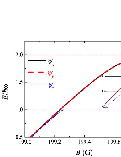
Figure 1: (Color online) The bound-state energy of two ⁴⁰K atoms in the $\left|F=\frac{9}{2},m_{F}=-\frac{7}{2}\right\rangle$ hyperfine state confined in a transversely isotropic waveguide near the $p$-wave Feshbach resonance centered at $B_{0}=198.8$G in three dimension Ticknor2004M ; Gunter2005P . The dotted horizontal lines are the thresholds that the bound states merge into the continuum as the magnetic field increases. The magnetic field $B$ dependence of the scattering volume $v_{1}$ as well as the effective range $r_{1}$ for ⁴⁰K is from Ref.Ticknor2004M . The insert shows the details of the curves in a smaller magnetic field range for eye clarity.

Figure 2: (Color online) The same as Fig.1 but for a transversely anisotropic confinement, i.e., $\eta=2$ .

III scattering solutions and confinement-induced resoannces

In this section, let us consider the low-energy $p$-wave scattering problem in the 1D waveguide with energy just above the transverse zero-point energy, i.e., $\epsilon\rightarrow 0^{+}$ . According to the Lippman-Schwinger equation, the scattering solution of the Hamiltonian (1) can formally be written as

$$\psi(\mathbf{r})=\psi_{0}\left(\mathbf{r}\right)-\int d^{3}\mathbf{r}^{\prime}G_{E}\left(\mathbf{r},\mathbf{r}^{\prime}\right)\mathcal{V}_{1}\left(\mathbf{r}^{\prime}\right)\psi\left(\mathbf{r}^{\prime}\right),$$ (25)

where $\psi_{0}\left(\mathbf{r}\right)$ is the incident wavefunction. Since the energy of the relative motion is just above the transverse zero-point energy, the atoms should enter from the transverse ground state, and the incident wavefunction takes the form of

$$\psi_{0}\left(\mathbf{r}\right)=\phi_{0}\left(\frac{\sqrt{\eta}x}{d}\right)\phi_{0}\left(\frac{y}{d}\right)i\sin\left(k_{z}z\right).$$ (26)

Here, we have considered the exchanging anti-symmetry of two identical fermions. Remind that $\phi_{0}\left(\cdot\right)$ is the 1D harmonic ground-state wavefunction and $k_{z}=\sqrt{2\epsilon}/d$ . The two-body Green’s function $G_{E}\left(\mathbf{r},\mathbf{r}^{\prime}\right)$ is the simple analytical continuation of Eq.(7) from $\epsilon<0$ to $\epsilon\approx 0^{+}$ . Substituting the $p$-wave pseudopotential (3) into Eq.(25), and at large separation, i.e., $r\rightarrow\infty$ , we find the scattering wavefunction (25) behaves as

$$\psi(\mathbf{r})\approx\phi_{0}\left(\frac{\sqrt{\eta}x}{d}\right)\phi_{0}\left(\frac{y}{d}\right)\times\\ \left[i\sin\left(k_{z}z\right)-\text{sgn}\left(z\right)\left(\frac{1}{v_{1}}-\frac{1}{2}r_{1}k^{2}\right)^{-1}\frac{\sqrt{\pi}\eta^{1/4}\mathcal{R}_{z}}{d}e^{ik_{z}\left|z\right|}\right],$$ (27)

where $\mathcal{R}_{z}$ is defined as in Eq.(9). For this 1D scattering problem in the waveguide, we anticipate the scattering wavefunction at large distance takes the form

$$\psi\left(\mathbf{r}\right)\sim\phi_{0}\left(\frac{\sqrt{\eta}x}{d}\right)\phi_{0}\left(\frac{y}{d}\right)\left[i\sin\left(k_{z}z\right)+\text{sgn}\left(z\right)f_{p}e^{ik_{z}\left|z\right|}\right],$$ (28)

where $f_{p}$ is the effective $p$-wave 1D scattering amplitude. Comparing Eqs.(27) and (28), we easily obtain the effective 1D scattering amplitude

$$f_{p}=-\left(\frac{1}{v_{1}}-\frac{1}{2}r_{1}k^{2}\right)^{-1}\frac{\sqrt{\pi}\eta^{1/4}\mathcal{R}_{z}}{d}.$$ (29)

The coefficient $\mathcal{R}_{z}$ is determined by the asymptotic behavior of the scattering wavefunction (25) at small distance, i.e., $r\approx 0$ , and we find

$$\mathcal{R}_{z}=\frac{i6k_{z}\eta^{1/4}}{\sqrt{\pi}d}\left[1+\frac{6}{\sqrt{\pi}d^{3}}\left(\frac{1}{v_{1}}-\frac{1}{2}r_{1}k^{2}\right)^{-1}\mathcal{F}_{z}^{\prime}\left(\epsilon,0\right)\right.\\ \left.+\frac{i6k_{z}\sqrt{\eta}}{d^{2}}\left(\frac{1}{v_{1}}-\frac{1}{2}r_{1}k^{2}\right)^{-1}\right]^{-1},$$ (30)

where

$$\mathcal{F}_{z}^{\prime}\left(\epsilon,0\right)=\int_{0}^{\infty}d\tau\left\{\frac{\sqrt{\eta}\exp\left(\epsilon\tau\right)}{\sqrt{2}\tau^{3/2}}\right.\\ \times\left[\frac{1}{\sqrt{\left(1-e^{-2\eta\tau}\right)\left(1-e^{-2\tau}\right)}}-1\right]-\\ \left.\left[\frac{1}{2\sqrt{2}\tau^{5/2}}+\frac{\epsilon+\left(\eta+1\right)/2-2\sqrt{\eta}}{2\sqrt{2}\tau^{3/2}}\right]\right\}.$$ (31)

For the low-energy 1D scattering problem, i.e., $k_{z}d\ll 1$ , it is convenient to use the effective 1D scattering lenght $l_{1D}$ to characterize scattering resonances, which can be defined from the scattering amplitude at zero energy ($\epsilon\approx 0^{+}$) as Pricoupenko2008R

$$f_{p}=-\frac{ik_{z}}{ik_{z}+l_{1D}^{-1}},$$ (32)

and

$$\frac{l_{1D}}{d}\equiv 6\sqrt{\eta}\left[\frac{d^{3}}{v_{1}}-dr_{1}\cdot\frac{\eta+1}{2}+\frac{6}{\sqrt{\pi}}\mathcal{F}_{z}^{\prime}\left(0,0\right)\right]^{-1}.$$ (33)

The divergence of the 1D scattering length $l_{1D}$ characterizes the scattering resonance in the waveguide. By tuning the 3D scattering volume $v_{1}$ and the effective range $r_{1}$ according to the $p$-wave Feshbach resonance, the $p$-wave CIR can be reached in the 1D waveguide when

$$\frac{d^{3}}{v_{1}}-dr_{1}\cdot\frac{\eta+1}{2}=-\frac{6}{\sqrt{\pi}}\mathcal{F}_{z}^{\prime}\left(0,0\right).$$ (34)

For a transversely isotropic confinement, i.e., $\eta=1$ , the 1D resonance condition (34) returns to the well-known result Granger2004T ; Pricoupenko2008R

$$\frac{d^{3}}{v_{1}}-dr_{1}=12\zeta\left(-\frac{1}{2}\right),$$ (35)

where $\zeta\left(\cdot\right)$ is the Riemann Zeta function, and note that we include the 3D $p$-wave effective range in our expression.

In Fig.3, we present the 1D scattering length $l_{1D}$ as function of the magnetic field strength $B$ in the waveguide with three typical transverse anisotropies $\eta=1,\,5,\,\text{and}\,10$. Here, we still consider two ⁴⁰K in the $\left|F=\frac{9}{2},m_{F}=-\frac{7}{2}\right\rangle$ hyperfine state near the $p$-wave Feshbach resonance centered at $B_{0}=198.8$G in 3D Ticknor2004M ; Gunter2005P . We find that, as the transverse anisotropy $\eta$ increases, the resonance position of $p$-wave CIR shifts to a higher magnetic field strength. More apparently, we show how the resonance position denoted by the magnetic field strength $B^{(R)}$ shifts with the transverse anisotropy $\eta$ in Fig.4.

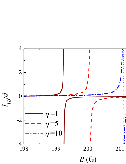
Figure 3: (Color online) The $p$-wave 1D scattering length $l_{1D}$ as functions of the magnetic field $B$ in the 1D waveguide with different transverse anisotropy $\eta$ . Here, the $p$-wave interaction of two ⁴⁰K atoms in the $\left|F=\frac{9}{2},m_{F}=-\frac{7}{2}\right\rangle$ hyperfine state is tuned by using the $p$-wave Feshbach resonance centered at $B_{0}=198.8$G in three dimension Ticknor2004M ; Gunter2005P .

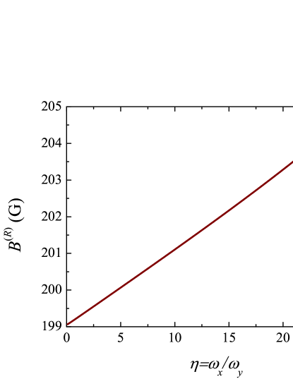
Figure 4: (Color online) The position of the $p$-wave confinement-induced resonance in the 1D waveguide denoted by the magnetic field strength $B^{(R)}$ as a function of the transverse anisotropy $\eta$ . In this plot, we tune the transversely anisotropy $\eta$ by increasing $\omega_{x}$ with fixed $\omega_{y}$ . The corresponding parameters are still from the ⁴⁰K experiments Ticknor2004M ; Gunter2005P .

IV The effective two-channel mechanism

For $s$-wave CIR in a quais-1D waveguide, there is a simple two-channel picutre first introduced by Bergeman el al. Bergeman2003A , and then extended to the case of the transversely anisotropic confinement Peng2010C . We may understand this two-channel mechanism as follows: due to the low temperature and tight transverse confinement, the two atoms can only enter from the transverse ground state, while the transverse excited modes are all closed. Therefore, the transverse ground state and the manifold of the remaining transverse excited states may be regarded as the open and closed channels, respectively. If a molecular state exists in the closed channel, a zero-energy scattering resonance occurs when this molecule energetically coincides with the continuum threshold of the open channel. In this section, we aim to study whether this simple two-channel picture is still valid for $p$-wave interaction.

Owing to the separability of c.m. motion and relative motion in harmonic traps, we still only focus on the relative-motion Hamiltonian (1). According to the two-channel mechanism proposed for $s$-wave interaction Bergeman2003A , the total relative-motion Hamiltonian $\mathcal{H}$ may formally be splitted into three terms, i.e., $\mathcal{H}_{op}$ , $\mathcal{H}_{cl}$ and $\mathcal{W}$ corresponding to the open channel, closed channel, and coupling part, respectively,

$$\mathcal{H} = \mathcal{H}_{op}+\mathcal{H}_{cl}+\mathcal{W}$$ (36)

$$\equiv P_{g}\mathcal{H}P_{g}+P_{e}\mathcal{H}P_{e}+\left(P_{g}\mathcal{H}P_{e}+H.c\right),$$

where $P_{g}=\left|g\right\rangle\left\langle g\right|$ , $P_{e}=\sum_{\alpha\neq g}\left|\alpha\right\rangle\left\langle\alpha\right|$ are the corresponding projection operators, and $\left|g\right\rangle$ , $\left|\alpha\right\rangle$ are the transverse ground and excited states, respectively. In the follows, we are going to show that the crossing of the molecular state in the closed channel $\mathcal{H}_{cl}$ and the energy continuum threshold of the open channel, i.e., $\hbar\omega\left(\eta+1\right)/2$ , denotes the position where the $p$-wave CIR occurs.

In order to obtain the molecular state of the closed channel, we need to solve the Schördinger equation $\mathcal{H}_{cl}\psi_{cl}\left(\mathbf{r}\right)=E\psi_{cl}\left(\mathbf{r}\right)$ . The procedure is similar to that of obtaining the bound states of the full Hamiltonian (1). However, we need to project out the transverse ground state, and this means the transverse ground state, i.e., the $n_{1}=n_{2}=0$ term, should be excluded in the expansion of the Green’s function, i. e., Eq.(6) . Similarly, we obtain the Green’s function for the closed channel Hamiltonian,

$$G_{E}^{(cl)}\left(\mathbf{r},\mathbf{r}^{\prime}\right)=\frac{\sqrt{\eta}}{\pi^{3/2}d^{3}\hbar\omega}\exp\left[-\frac{\eta\left(x^{2}+x^{\prime 2}\right)+y^{2}+y^{\prime 2}}{2d^{2}}\right]\int_{0}^{\infty}d\tau\frac{e^{\epsilon\tau}}{\sqrt{2\tau}}\exp\left[-\frac{\left(z-z^{\prime}\right)^{2}}{2d^{2}\tau}\right]\\ \times\left\{\frac{\exp\left[\eta\frac{2xx^{\prime}-\left(x^{\prime 2}+x^{2}\right)e^{-\eta\tau}}{2d^{2}\sinh\left(\eta\tau\right)}+\frac{2yy^{\prime}-\left(y^{\prime 2}+y^{2}\right)e^{-\tau}}{2d^{2}\sinh\tau}\right]}{\sqrt{\left(1-e^{-2\eta\tau}\right)\left(1-e^{-2\tau}\right)}}-1\right\}.$$ (37)

Then the bound-state wavefunction $\psi_{cl}\left(\mathbf{r}\right)$ takes the form

$$\psi_{cl}\left(\mathbf{r}\right)=-\frac{\pi\hbar^{2}}{\mu}\left(\frac{1}{v_{1}}-\frac{1}{2}r_{1}k^{2}\right)^{-1}\\ \cdot\sum_{n}\mathcal{R}_{n}^{\prime}\left[\frac{\partial}{\partial r_{n}^{\prime}}G_{E}^{(cl)}\left(\mathbf{r},\mathbf{r}^{\prime}\right)\right]_{r^{\prime}=0},$$ (38)

where

$$\mathcal{R}_{n}^{\prime}\equiv\left[\frac{\partial^{3}}{\partial r^{3}}r^{3}\frac{\partial}{\partial r_{n}}\psi_{cl}\left(\mathbf{r}\right)\right].$$ (39)

After straightforward and similar algebra as that in Sec.II, we find there are also three bound states in the closed channel, and two of them are with odd transverse parity, while that of the third is even, which takes the form,

$$\psi_{cl,z}\left(\mathbf{r}\right)=z\left[\frac{1}{r^{3}}+\frac{E}{\hbar\omega}\frac{1}{rd^{2}}+\frac{2}{\sqrt{\pi}d^{3}}\mathcal{F}_{z}^{\prime}\left(\epsilon,\mathbf{r}\right)\right],$$ (40)

where

$$\mathcal{F}_{z}^{\prime}\left(\epsilon,\mathbf{r}\right)=\int_{0}^{\infty}d\tau\left\{\frac{\sqrt{\eta}\exp\left(\epsilon\tau-\frac{z^{2}}{2d^{2}\tau}-\frac{\eta x^{2}+y^{2}}{2d^{2}}\right)}{\sqrt{2}\tau^{3/2}}\left[\frac{\exp\left(-\frac{\eta x^{2}e^{-\eta\tau}}{2d^{2}\sinh\left(\eta\tau\right)}-\frac{y^{2}e^{-\tau}}{2d^{2}\sinh\tau}\right)}{\sqrt{\left(1-e^{-2\eta\tau}\right)\left(1-e^{-2\tau}\right)}}-1\right]-\right.\\ \left.\frac{1}{2\sqrt{2}}\left[\frac{1}{\tau^{5/2}}+\left(\frac{E}{\hbar\omega}-2\sqrt{\eta}\right)\frac{1}{\tau^{3/2}}\right]e^{-\frac{r^{2}}{2d^{2}\tau}}\right\}.$$ (41)

The corresponding binding energy of the bound state with even transverse parity satisfies,

$$\frac{d^{3}}{v_{1}}=-\frac{6}{\sqrt{\pi}}\mathcal{F}_{z}^{\prime}\left(\epsilon,0\right)+dr_{1}\cdot\frac{E}{\hbar\omega}.$$ (42)

Obviously, $\mathcal{F}_{z}^{\prime}\left(\epsilon,0\right)$ takes the form of Eq.(31). If two atoms enter from the transverse ground state (open channel) with energy below the transverse excited states (closed channel), they may only be coupled to the molecular state $\psi_{cl,z}\left(\mathbf{r}\right)$ with even transverse parity, due to the parity conservation. When this molecular state energetically crosses the continuum threshold of the open channel ($\epsilon\approx 0$), a zero-energy scattering resonance occurs. From Eq.(40), the resonance condition is given by

$$\frac{d^{3}}{v_{1}}-dr_{1}\cdot\frac{\eta+1}{2}=-\frac{6}{\sqrt{\pi}}\mathcal{F}_{z}^{\prime}\left(0,0\right),$$ (43)

which returns to Eq.(34) again. The binding energy of the ⁴⁰K-⁴⁰K molecular state $\psi_{cl,z}\left(\mathbf{r}\right)$ in the closed channel $\mathcal{H}_{cl}$ under different transverse anisotropy is illustrated in Fig.5, and the interatomic interaction is still tuned by $p$-wave Feshbach resonance centered at $B_{0}=198.8$G. The vertical dashed lines indicate where the $p$-wave CIR occurs.

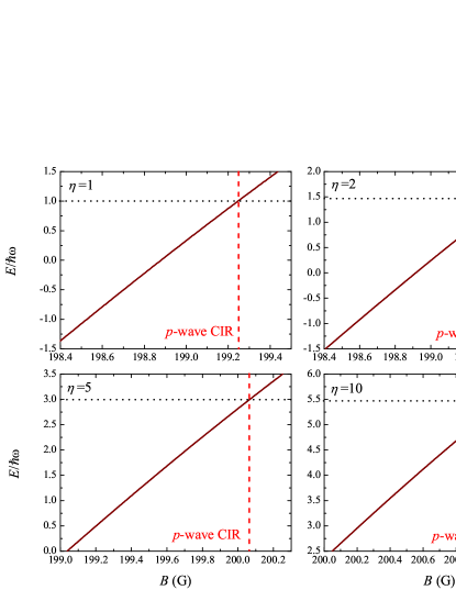
Figure 5: (Color online) The molecular state of the closed channel Hamiltonian $\mathcal{H}_{cl}$ for different transverse anisotropy $\eta$ . The horizontal dotted lines denote the continuum threshold of the open channel, while the vertical red dashed lines indicate the position where a zero-energy scattering resonance occurs.

V Conclusions

We theoretically investigate the influence of the transverse anisotropy of the confinement on the two-body state with $p$-wave interaction in a quasi-one-dimensional waveguide. The two-body problem in such quasi-one-dimensional systems is solved. The interatomic interaction is modeled by $p$-wave pseudopotential. We find there are totally three bound states due to the non-zero orbital angular momentum of $p$-wave interaction, while there is only one two-body bound state supported by $s$-wave pseudopotential. In addition, the effective one-dimensional scattering amplitude and scattering length are derived. We predict the $p$-wave confinement-induced resonance for any transverse anisotropy of the waveguide, whose position shows an apparent shift with increasing transverse anisotropy. Besides, a two-channel mechanism is presented for $p$-wave confinement-induced resonance in a waveguide, which was first proposed for $s$-wave interaction. We find this effective two-channel picture is still valid for $p$-wave interaction. All our calculations are based on the parameterization of the ⁴⁰K experiments, and can be confirmed in future experiements.

References

• (1) M.Olshanii, Physical Review Letters 81, 938 (1998).
• (2) D. S. Petrov, M. Holzmann, and G. V. Shlyapnikov, Physical Review Letters 84, 2551 (2000).
• (3) D. S. Petrov and G. V. Shlyapnikov, Physical Review A 64, 012706 (2001).
• (4) T. Bergeman, M. G. Moore, and M. Olshanii, Physical Review Letters 91, 163201 (2003).
• (5) B. E. Granger and D. Blume, Physical Review Letters 92, 133202 (2004).
• (6) H. Moritz, T. Stoferle, K. Gunter, M. Kohl, and T. Esslinger, Physical Review Letters 94, 210401 (2005).
• (7) K. Gunter, T. Stoferle, H. Moritz, M. Kohl, and T. Esslinger, Physical Review Letters 95, 230401 (2005).
• (8) L. Pricoupenko, Physical Review Letters 100, 170404 (2008).
• (9) E. Haller, M. Gustavsson, M. J. Mark, J. G. Danzl, R. Hart, G. Pupillo, and H. C. NΓ€gerl, Science 325, 1224 (2009).
• (10) E. Haller, M. J. Mark, R. Hart, J. G. Danzl, L. ReichsΓΆllner, V. Melezhik, P. Schmelcher, and H. C. NΓ€gerl, Physical Review Letters 104, 153203 (2010).
• (11) B. Frohlich, M. Feld, E. Vogt, M. Koschorreck, W. Zwerger, and M. Kohl, Physical Review Letters 106, 105301 (2011).
• (12) S.-G. Peng, S. S. Bohloul, X.-J. Liu, H. Hu, and P. D. Drummond, Physical Review A 82, 063633 (2010).
• (13) W. Zhang and P. Zhang, Physical Review A 83, 13 (2011).
• (14) S. G. Peng, H. Hu, X. J. Liu, and P. D. Drummond, Physical Review A 84, 043619 (2011).
• (15) S. Sala, P.-I. Schneider, and A. Saenz, Physical Review Letters 109, 073201 (2012).
• (16) P. Giannakeas, V. S. Melezhik, and P. Schmelcher, Physical Review A 84, 023618 (2011).
• (17) S. G. Peng, H. Hu, X. J. Liu, and K. J. Jiang, Physical Review A 86, 033601 (2012).
• (18) S.-G. Peng, S. Tan, and K. Jiang, Physical Review Letters 112, 250401 (2014).
• (19) Y. Ohashi, Physical Review Letters 94, 050403 (2005).
• (20) T. L. Ho and R. B. Diener, Physical Review Letters 94, 090402 (2005).
• (21) C. H. Cheng and S. K. Yip, Physical Review Letters 95, 070404 (2005).
• (22) M. Iskin and C. de Melo, Physical Review Letters 96, 040402 (2006).
• (23) J. Zhang, et al., Physical Review A 70, 030702 (2004).
• (24) C. Ticknor, C. A. Regal, D. S. Jin, and J. L. Bohn, Physical Review A 69, 042712 (2004).
• (25) S. G. Peng, S. Q. Li, P. D. Drummond, and X. J. Liu, Physical Review A 83, 063618 (2011).
• (26) S. K. Yip, Physical Review A 78, 013612 (2008).
• (27) A. Suzuki, Y. Liang, and R. K. Bhaduri, Physical Review A 80, 033601 (2009).
• (28) Z. Idziaszek, Physical Review A 79, 062701 (2009).