Multi-wavelength observations of the black widow pulsar 2FGL J2339.6$-$0532 with OISTER and Suzaku

Abstract

Multi-wavelength observations of the black-widow binary system 2FGL J2339.6$-$0532 are reported. The Fermi gamma-ray source 2FGL J2339.6-0532 was recently categorized as a black widow in which a recycled millisecond pulsar (MSP) is evaporating up the companion star with its powerful pulsar wind. Our optical observations show clear sinusoidal light curves due to the asymmetric temperature distribution of the companion star. Assuming a simple geometry, we constrained the range of the inclination angle of the binary system to $52\arcdeg<i<59\arcdeg$, which enables us to discuss the interaction between the pulsar wind and the companion in detail. The X-ray spectrum consists of two components: a soft, steady component that seems to originate from the surface of the MSP, and a hard variable component from the wind-termination shock near the companion star. The measured X-ray luminosity is comparable to the bolometric luminosity of the companion, meaning that the heating efficiency is less than 0.5. In the companion orbit, $10^{11}$ cm from the pulsar, the pulsar wind is already in particle dominant-stage, with a magnetization parameter of $\sigma<0.1$. In addition, we precisely investigated the time variations of the X-ray periodograms and detected a weakening of orbital modulation. The observed phenomenon may be related to an unstable pulsar-wind activity or a weak mass accretion, both of which can result in the temporal extinction of radio-pulse.

1. Introduction

A milli-second pulsar (MSP) is believed to evolve from a dead pulsar in a binary system, via mass accretion from a companion star that has spun up the pulsar for billions of years (Alpar et al., 1982). Indeed most MSPs are discovered in binary systems, however isolated MSPs also exist. The missing link between the isolated MSPs and binary MSPs is black widow pulsars in which a sufficiently spun up pulsar is evaporating its companion star with its powerful pulsar wind. The prototype of the black widow is PSR B1957$+$20 with a 1.61 ms radio pulse (Fruchter et al., 1988). So far less than 10 black widow class objects have been discovered however the evolution process from an accreting MSP to a rotation-powered MSP is still unclear(Roberts, 2011, 2013).

Moreover a black widow may be a good probe for deep investigation of pulsar wind. Currently young rotation powered pulsars are believed to have pulsar wind nebulae (PWNe) made up of relativistic electron-positron plasma, as seen in the Crab nebula (Weisskopf et al., 2000; Hester et al., 2002), however the physical mechanism that generates the pulsar wind is not yet understood. Although we do not know whether the descriptions of the Crab pulsar can be applied to a recycled MSP with magnetic field four orders of magnitude weaker than that of typical radio pulsars, if this is the case, the black widows can provide a crucial chance for us to probe pulsar wind via the direct interaction with the companion nearby the light cylinder. Theoretically pulsar wind is dominated by Poynting flux at the light cylinder, therefore the magnetic energy in the wind must be converted into kinetic energy just after the wind flies out from the light cylinder as reported by Aharonian et al. (2012), and we can approach the origin of the pulsar wind much deeper with black widows for investigating the unknown physical mechanism which can explain the $\sigma$ paradox. In order to clarify the history of MSP formation and also to constrain the physical mechanism of particle acceleration “just” around the pulsar, a black widow pulsar is an intriguing target.

The Large Area Telescope (LAT) on the Fermi satellite, with unprecedented sensitivity and angular resolution in the energy range of 100 MeV to greater than 300 GeV, has discovered more than 2000 gamma-ray sources since its launch, and 30% of these sources are still unidentified. A bright gamma-ray source discovered at high galactic latitude vicinity, 2FGL J2339.6$-$0532 (1FGL J 2339.7$-$0531), was also listed in the first Fermi source catalog as an un-identified source (Abdo et al., 2010; Ackermann et al., 2012). The gamma-ray flux amounts to $3.0\pm 0.2\times 10^{-11}$ erg s^-1 cm^-2 with a variable index of 15.7, indicating that the gamma-ray flux seems to be steady at the month time scale. While the gamma-ray spectrum has a cutoff structure at 3 GeV. These characteristics lead us to believe the object is a pulsar. A follow-up X-ray observation conducted with Chandra discovered an X-ray point source within the error circle expected from the gamma-ray image(Kong et al., 2012). However a radio pulse was not detected at the position at that moment. On the other hand, ground based optical observations discovered clear sinusoidal variability with a period of 4.63 hours, which implies the object is in a binary system and the observed optical variability is likely related to the orbital motion. The intensity of the optical counterpart varies from 20 to 17 mag in R-band(Romani & Shaw, 2011; Kong et al., 2012). Moreover the phase-resolved spectroscopy indicated that the companion may be K-class star with a mass of 0.075 $M_{\sun}$. This means that the pulsar side hemisphere of the companion star is drastically heated and the energy might be supplied from an unknown recycled MSP via pulsar wind, as seen in PSR B1957$+$20.

In this paper, we report multi-wavelength observations of the newly discovered black widow binary system 2FGL J2339.6-0532, covering near-infrared, optical and X-ray energy band. In section 2 and 3, the optical and X-ray observations and the obtained results are described, respectively. In section 4, we discuss the orbital parameters based on the obtained phase resolved SED and the properties of the pulsar wind just around the pulsar as well as an interpretation of the X-ray light curve showing intriguing irregular variability.

2. Optical observations

2.1. Observation

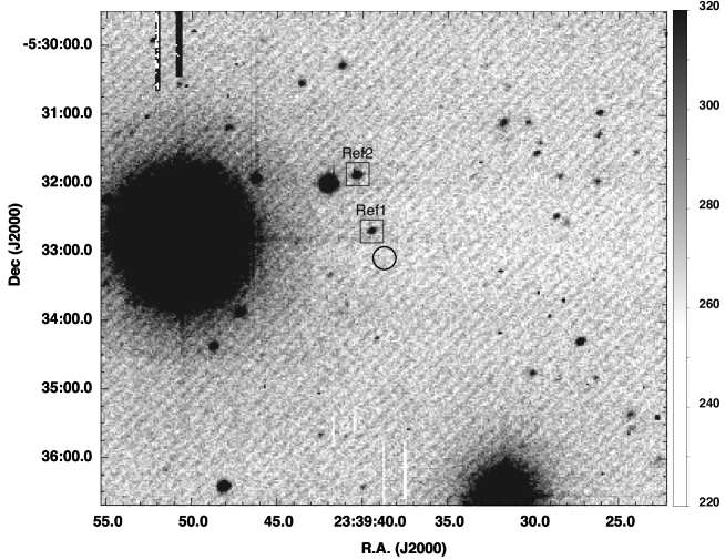
Figure 1.— H$\alpha$ image of the vicinity of 2FGL J2339.6$-$0532 observed with the Kiso-105cm Schmidt telescope. The circle region with a radius of 10″indicates the location of the target. Two rectangular regions indicate the photometric reference stars shown in Table 1.

2FGL J2339.6$-$0532 was observed from September 22 to October 7 2011 utilizing the global telescope network, “Optical and Infrared Synergetic Telescopes for Education and Research (OISTER)” . OISTER consists of 14 independent observatories that are funded by Japanese universities and research associations. For this work, we also asked for photometry observation from the Kottamia Astronomical observatory which has a 188 cm reflector. Thanks to the locations of the observatories distributed across the globe, we can continuously trace the variability all day long. Moreover the telescopes cover a wide range of wavelengths from Ks to B band which can provides phase resolved spectral energy distribution (SED) of the target. The conducted photometric observations are summarized in Table 4. The locations of the reference stars and the target are shown in Figure 1.

2.2. H$\alpha$ imaging

In the case of PSR B1957$+$20, the binary system is surrounded by an H$\alpha$ bow-shock due to its super sonic proper motion with respect to the surrounding ISM (Kulkarni & Hester, 1988). To search for a similar feature around 2FGL J2339.6-0532, we took H$\alpha$ images with the Kiso Schmidt telescope at the minimum phase to prevent contamination from the companion star. Figure 1 shows the obtained H$\alpha$ image in the vicinity of 2FGL J2339.6-0532 utilizing an H$\alpha$ narrow band filter ($\Delta\lambda=9$ nm), in which we could not find the evidence of bow-shock nebula.

To evaluate the detection limit, we calculated the standard deviation of the 33″$\times 67\arcsec$ (50$\times$100 pixel) rectangular region near the target and obtained $STDEV=7.82$ ADU. The sky background of the CCD image shows a weak striped pattern running in the southeast-to-northwest direction, with a peak-to-peak value of $\sim 8$ ADU, which seems to be the dominant noise component restricting the detection limit. Regardless, if we adopt a conservative threshold with a 3$\sigma$ confidence level, the detection limit becomes 23.5 ADU. Based on the flux calibrations of the reference stars listed in Table 1, the conversion coefficient of ADU to energy flux, $(8.3\pm 0.1)\times 10^{-18}$ erg s^-1 cm^-2 ADU^-1, was observed for the H$\alpha$ filter with a bandwidth of 9 nm. Finally, we obtained a 3$\sigma$ detection limit of $<1.9\times 10^{-16}$ erg s^-1 cm^-2 pixel^-1, which corresponds to a surface brightness of $<8.7\times 10^{-17}$ erg s^-1 cm^-2 arcsec^-2  .

Table 1Summary of Field photometry

	Reference-1	Reference-2	A${}_{\lambda}\tablenotemark{$\dagger$}$
Name(USNO-2.0A)	U0825_19993817	U0825_19993871
Coordinate(J2000.0)	(23:39:39.487, $-$05:32:40.56)	(23:39:40.366, $-$05:31:51.89)
B	$18.435\pm 0.014$	$17.603\pm 0.008$	0.120
V	$17.834\pm 0.018$	$16.828\pm 0.008$	0.091
R	$17.484\pm 0.016$	$16.388\pm 0.007$	0.072
I	$17.296\pm 0.020$	$16.105\pm 0.008$	0.050
g’	$18.098\pm 0.011$	$17.177\pm 0.006$	0.110
J	$16.47\pm 0.10$	$15.19\pm 0.04$	0.024
H	$16.45\pm 0.23$	$14.87\pm 0.05$	0.015
Ks	$16.12$	$14.55\pm 0.08$	0.011
H$\alpha$ (656 nm)	$314\pm 46\quad\mu$Jy	$854\pm 170\quad\mu$Jy	$\cdots$

.

Note. — Errors are with 1$\sigma$ confidence level.

The prototype black widow PSR B1957+20, residing at a distance of 1.6 kpc from the earth, has a bow-shock nebula extending over $\sim$ 30″$\times$ 30″with an H$\alpha$ flux of $3.3\times 10^{-14}$ erg s^-1 integrated over the entire nebula (Kulkarni & Hester, 1988). If our target is accompanied by an equivalent bow-shock nebula, the H$\alpha$ flux and the size should be $6.1\times 10^{-14}$ erg s^-1 cm^-2 and $\sim 41\arcsec\times 41\arcsec$, respectively. Therefore, the expected surface brightness is $3.6\times 10^{-17}$ erg s^-1 cm^-2 arcsec^-2, which is slightly lower than the detection limit.

Compared with the other bow-shock PWNe, the size and intensity both seem to be scattered across a range of two orders of magnitude, possibly reflecting their shock conditions (Chatterjee & Cordes, 2002). Therefore, we conclude that this observation provides only a weak upper limit of surface brightness in the H$\alpha$ band.

2.3. Photometry

The other telescopes except for the Kiso observatory carried out photometric observations covering Ks$\sim$B bands from September 9th 2011 to September 30th 2011. For flux calibration we chose two reference stars near the target object, U0825_19993817 (R=17.5) and U0825_19993871 (R=16.4) in USNO-2.0A catalog, so that all of the observatories can employ the common references without saturation. The photon fluxes of the references stars were measured and compared to the standard stars in the Landolt catalog (Landolt, 1992) with MSI of the Pirka telescope in Hokkaido prefecture (Japan). Since the Pirka employs the Johnson-Cousins filter system, we estimated the photon flux in the SDSS g’-band based on the observed B and V magnitudes using a conversion equation proposed by Smith et al. (2002),

$$g^{\prime}=V+0.54(B-V)-0.07.$$ (1)

For J, H, and Ks, we employed the photometric data in the Two Million All Sky Survey (2MASS) catalog for flux calibration (Skrutskie et al., 2006). The obtained magnitude of the reference stars are summarized in Table 1.

Figure 2 shows the light curves of 2FGL J2339.6$-$0532 obtained by OISTER. We re-confirmed the clear sinusoidal modulation as reported by Kong et al. (2012) and Romani & Shaw (2011). The absolute flux seems consistent with the past observations: the modulation amplitude is about 4.5 magnitude in the R-band and is larger at shorter wavelength. In R-band, we successfully observed the maximum phases of the target 8 times during the observation campaign. The photon flux at the maximum phase is $R_{\rm max}=17.7$ mag on average and varies among peaks within a range of $\pm 0.1$ mag. There was no irregular activity like the flares observed in 2FGL J1311.6$-$3429 (Kataoka et al., 2012).

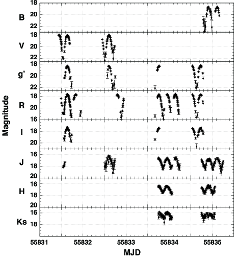
Figure 2.— Multi-color light curve of 2FGL J2339.6$-$0532 obtained via OISTER.

2.4. Phase-resolved SED

To discuss the energetics quantitatively, we estimated the energy flux based on the photometric data shown in Figure 2. First we corrected the galactic extinction at the coordinate of the target (Schlafly & Finkbeiner, 2011; Cardelli et al., 1989); the employed extinction at various wavelength are listed in Table 1. Then we converted the absorption corrected magnitudes to energy flux using conversion equations presented in Fukugita et al. (1996) and Tokunaga & Vacca (2005) for optical (B, V, R, I, g’) and IR(J, H, Ks) energy bands, respectively.

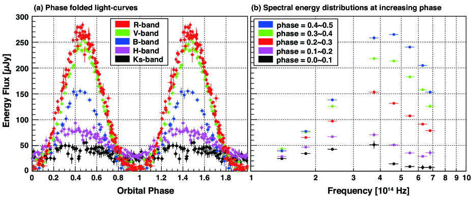
Figure 3.— (a)Phase folded multi-color light curves. The assumed orbital period is 4.63435 hr and Phase=0 is set to be MJD=55500 day. Marker colors represent the energy bands: red= R, green= V, blue=B, magenta=H, and black=Ks. (b)Spectral energy distributions at increasing phase from the minimum to the maximum. Colors correspond to the orbital phase: black=0-0.1, magenta=0.1-0.2, red=0.2-0.3, green=0.3-0.4, and blue=0.4-0.5.

Figure 3—(a) shows the yielded energy fluxes as functions of the binary orbital phase. Phase=0 was set to be MJD=55500.0. While the optical light-curves show symmetric structures, IR (H and Ks) light-curves possess somewhat asymmetric shapes. This may be due to the geometry of the companion star or evaporating stellar gas. Panel (b) shows the spectral energy distribution during the brightening phase from orbital phase= 0 to 0.5 in panel (a). Clearly the peak frequency increases as the orbital phase increases from orbital phase 0 to 0.5, implying that the temperature of the companion is increasing with the orbital phase. At the maximum phase the SED is fitted with a black-body model with an effective temperature of $T_{\rm eff}=7540\pm 130$ K, which is consistent with the past study (Romani & Shaw, 2011).

In this paper, we assumed a simple emission model from the surface of the companion star to explain the observed optical emission. As described in Figure 4, we supposed that a companion star with a radius $r_{\rm comp}$ is orbiting around a pulsar at an orbital radius $R_{\rm orb}$, and the hemisphere of the companion that faces the pulsar is heated by the pulsar wind, while the opposite side of the companion has ordinal temperature $T_{\rm cool}$. Note that this model does not take into account the effect of energy transfer via convection or advection on the surface of the companion, therefore the temperature distribution of the companion is simply described by the energy injection via pulsar wind although the heating efficiency is unclear. In this paper, we assumed that the spin-down energy is perfectly converted into the isotropic pulsar wind and the injected energy via the pulsar wind heats the companion up with a heating efficiency of $f$ for simplicity. We also adopted a spin-down luminosity of $2.3\times 10^{34}$ erg s^-1 based on the timing analysis in radio band recently reported by Ray et al. (2014).

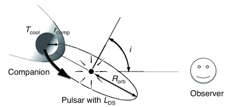
Figure 4.— Schematic image of the assumed emission model in which a companion star with a radius $r_{\rm comp}$ is orbiting around a pulsar at an orbital radius $R_{\rm orb}$. The hemisphere of the companion star facing the pulsar is heated. In this paper, the inclination angle $i$ is defined as the angle between the line of sight and the normal line to the orbital plane.

We then fitted the obtained phase-resolved SED with the model function described above (Figure 5). Since the model seems to correlate weakly with the inclination angle, we fixed the inclination angle $i$. The resultant model parameters are summarized in Figure 6 as functions of inclination angle. Although the fit seems rather poor — mainly because of the large residual in the IR band — we found that an inclination angle $i=59\arcdeg$ minimizes the $\chi^{2}$. For comparison, we also attempted this analysis without IR data and obtained a best-fit parameter of $i=52\arcdeg$. These results seem consistent with the inclination angle reported by Romani & Shaw (2011). The obtained best-fit parameters are summarized in Table 2. Additionally, the obtained temperature distributions of the companion surface are plotted in Figure 7 as functions of the zenith angle of the pulsar from the measured point on the companion surface.

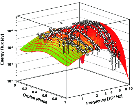
Figure 5.— Phase-resolved SED fitted with a model function.

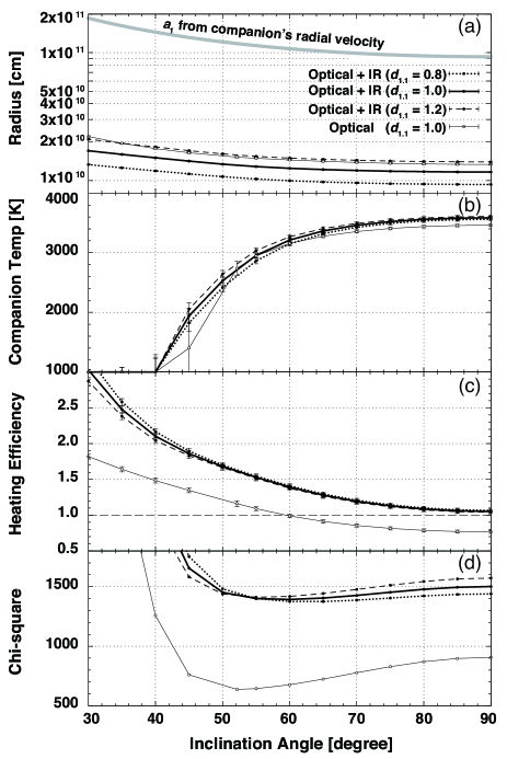
Figure 6.— The obtained parameters from model-fitting of the phase-resolved SED as functions of inclination angle$i$. Panel (a)$\sim$(d) show the orbital radius $R_{\rm orb}$ and companion radius $r_{\rm comp}$, the companion temperature at the cool side, the heating efficiency $f$, and the resultant $\chi^{2}$ (d.o.f = 901), respectively. The gray-bold line on panel (a) represents the semi-major axis of the companion calculated from the radial velocity of 350 km s^-1 with respect to the mass centroid of the system (Romani & Shaw, 2011). In this calculation we employed a spin-down luminosity of the pulsar, $L_{\rm SD}=2.3\times 10^{34}$, based on Ray et al. (2014).

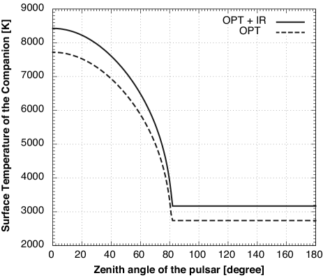
Figure 7.— Simulated temperature of the companion surface as a function of zenith angle of the pulsar from the position for which the calculation is performed. The simulations were performed for the best-fit parameters listed in Table 2.

Table 2Obtained parameters of the binary system from the phase-resolved SED

Data set	Optical+IR	Optical
Orbital radius ($R_{\rm orb}$)	$1.08\pm 0.02\quad\times 10^{11}$ cm	$1.18\pm 0.02\quad\times 10^{11}$ cm
Companion radius ($r_{\rm comp}$)	$1.26\pm 0.02\quad\times 10^{10}\;d_{\rm 1.1}$ cm	$1.53\pm 0.02\quad\times 10^{10}\;d_{\rm 1.1}$ cm
Companion Temperature ($T_{\rm cool}$)	$3170\pm 70\quad$ K	$2740\pm 120\quad$ K
Heating Efficiency ($f$)	$1.42\pm 0.05$	$1.16\pm 0.04$
Inclination angle ($i$)	$59.\arcdeg 0\pm 1.\arcdeg 5$	$52.\arcdeg 1\pm 1.\arcdeg 0$
Bolometric Luminosity	$1.09\pm 0.17\quad\times 10^{32}\;d_{\rm 1.1}^{2}$ erg s-1	$1.12\pm 0.16\quad\times 10^{32}\;d_{\rm 1.1}^{2}$ erg s-1
$\chi^{2}$	1392.6	637.6

Note. — Errors are with 1 $\sigma$ confidence level.

3. X-ray observation

3.1. Observation

2FGL J2339.6$-$05312 was observed with the Suzaku satellite on Jun. 29th, 2011. The target was observed at the XIS nominal point with the normal imaging mode. The net exposure time after the standard data reduction process was 96 ks. The accumulated photons are 2555 counts with the front-illuminated CCDs (XIS0 + XIS3) and 1874 counts with the back-illuminated CCD (XIS1) in the 0.4$-$8 keV energy band. During the observation, the event rates were $\sim 8.25\pm 0.28\times 10^{-3}$ (XIS0, XIS3) photons s^-1 and $8.89\pm 0.50\times 10^{-3}$ photons s^-1 (XIS1) in the energy band.

3.2. Spectral analysis

Figure 8 shows the X-ray spectrum obtained with the Suzaku. At first, we tried to fit the X-ray spectra with a single power-law function however the resultant fit was poor ($\chi^{2}/\nu$ = 67.71/55) due to residuals below 1 keV, implying the presence of a soft excess component. We therefore added a black-body to the model function for the soft excess, and obtained a better fit ($\chi^{2}/\nu=51.82/55$). Dotted lines on Figure 8 describe the best-fit model functions. The resultant parameters of the model fitting are summarized in Table 3. In both case, the column density converged on zero. The resultant upper limit is $<1.2\times 10^{21}$ cm^-2 with 90 % confidence level, and is consistent with the Galactic absorption of $3.23\times 10^{20}$ cm² for this direction (Dickey & Lockman, 1990; Kalberla et al., 2005).

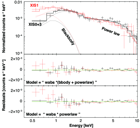
Figure 8.— X-ray spectra observed by the XIS aboard the Suzaku satellite. Black and red data points corresponds to the spectra observed with the front illuminated CCDs (XIS0 and XIS3), and with the back illuminated CCD (XIS1), respectively. Dotted-lines show the best-fit model functions consisting of a low-temperature black-body and a power-law function. The model parameters are found in Table 3.

Table 3Results of model fitting of the averaged X-ray spectra

Model	wabs*(bbody + power-law)	wabs*power-law
$N_{\rm H}$ ($10^{21}$ cm-2)	$<1.2$ (0)	$<0.13$ (0)
Blackbody Temperature (keV)	$0.15\pm 0.06$	$\cdots$
Blackbody Radius (km)	$0.28^{+0.93}_{-0.16}\quad$	$\cdots$
Power-law Photon Index	$1.14^{+0.14}_{-0.15}$	$1.32\pm 0.08$
Power-law Flux0.5-10keV ($10^{-13}$ erg cm-2 s-1)	$2.50\pm 0.16$	$2.50\pm 0.15$
Total flux0.5-10keV ($10^{-13}$erg cm-2 s-1)	$2.67^{+0.01}_{-1.25}$	$2.46^{+0.04}_{-0.73}$
$\chi^{2}$ (dof)	51.82 (51)	67.71(53)

Note. — Errors are with 90 % confidence level.

In order to clarify the origin of these two components, phase-folded X-ray light curves were generated as shown in Figure 9. In this figure, Phase=0 was set to be MJD=55500.0 in the same way as the optical light curves shown in Figure 3$-$(a). Panel (a)$\sim$(c) in Figure 9 represent the energy bands 0.4$-$1.0 keV, 2.0$-$4.0 keV and 4.0$-$8.0 keV, respectively. Clearly, the hard X-ray light curves show clear modulation coinciding with the orbital motion. This timing coincidence may imply that the non-thermal emission originates from the companion surface. However the shape of the light curves is somewhat different from the sinusoidal shapes observed in optical, i.e., a double-peaked shape at 2.0$-$4.0 keV band, and a flat top shape at 4.0$-$8.0 keV. On the other hand, the soft X-rays seem to be steady. This may imply that the soft component has a different emitting region, namely the pulsar.

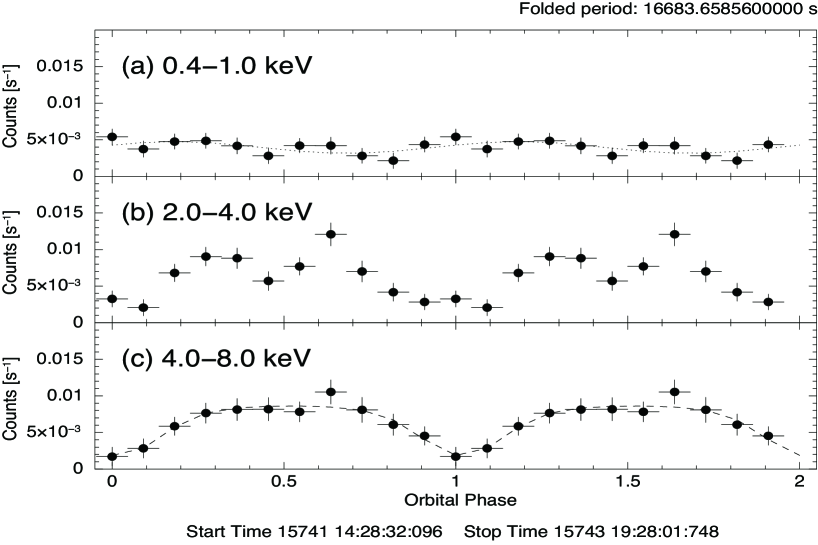
Figure 9.— Phase-folded X-ray light curves for (a)0.4$-$1.0 keV (b)2.0$-$4.0 keV and (c)4.0$-$8.0 keV energy bands. Phase=0 is set to be MJD=55500.0 in the same way as the optical light curves. Dotted line in panel (a) is the best-fit sinusoidal curve for evaluating the modulation factor. Dashed line in panel (c) shows a model function for synchrotron emission from a thin layer covering the companion hemisphere.

To evaluate the upper limit of the modulation factor in the soft X-ray energy band, we tried to fit the X-ray light curve with a sinusoidal curve and a constant component, $A\sin(2\pi x)+B$, where $x$ is the orbital phase. The obtained amplitude of the sinusoidal curve is $A=(0.80\pm 0.34)\times 10^{-3}$ counts s^-1 against the constant component of $B=(3.95\pm 0.23)\times 10^{-3}$ counts s^-1. Therefore, the upper limit of the modulation factor is $A/B<28.6$% with 1 $\sigma$ confidence level. Note that the maximum point was not fixed to be phase=0.5 in this estimation; this helped to maximize the modulation factor. The best-fit model curve is shown in Figure 9 (a).

If we adopt the two-component model consisting of a blackbody and a power-law function from the X-ray spectroscopy, we can roughly evaluate the contributions from these two components to the constant emission. The phase-averaged absorbed-photon flux for the blackbody and the power law in the 0.4$-$1.0 keV energy band are both $2.0\times 10^{-5}$ photons s^-1. Assuming that the constant component originates in the blackbody, the modulation factor is expected to be $(PL)/(BB+PL)\sim 50$ %, which is about twice of the measured value. Taking into account the large errors arising from the uncertainties of the blackbody components (see Table 3), the measured modulation factor should be larger because of the tight upper limits to the blackbody component. This may indicate that the constant emission may consist of the blackbody from the NS surface and the non-thermal component originating in the pulsar magnetosphere.

3.3. Temporal analysis

The upper panel of Figure 10 shows the obtained X-ray light curve with a bin size of 600 s for the energy range of 0.4$-$8.0 keV. Note that the whole length of the light curve is 190 ks, containing occultation periods of earth, and corresponding to the twice of the net exposure time of 96 ks. Although the photon statistics seem poor, the X-rays show periodic variability coincident with an orbital period of 16683 s. We expected to observe the flare-like features reported in previous studies (Kataoka et al., 2012; Papitto et al., 2013; Ferrigno et al., 2014; Linares et al., 2014), which may be related to the accretion activity; however, no significant evidence for this was discovered. Nonetheless, the shapes of the light curve seem to change over time.

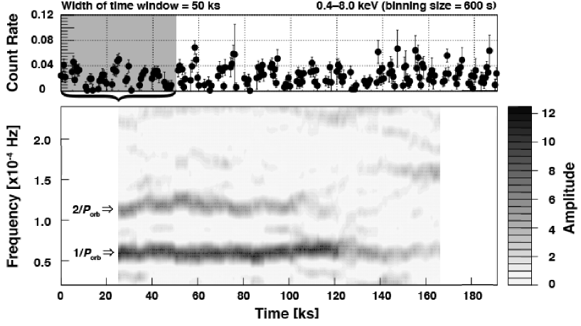
Figure 10.— Upper panel shows the X-ray light curve for energy band of 0.4$-$8.0 keV with a bin size of 600 s. Lower panel shows the running periodogram generated from the X-ray light curve shown in the upper panel with the Lomb-Scargle algorithm. We employed a 50ks rectangular window function that scans over the entire X-ray light curve of 190 ks. The horizontal line in the lower panel corresponds to the center time of the sampled time span of 50 ks. The gray scale shows arbitrary amplitude of modulation. Note that the amplitude of 6.3 correspond to 90 % confidence level.

In order to clarify the temporal variation in the waveform of the X-ray light curve, we traced the temporal changes of the power spectrum with the Lomb-Scargle algorithm, which can be applied to an unevenly sampled data set. In this analysis, we employed a rectangular function as a window function to detect small changes from a short data sequence. The width of window function was set to 50 ks in order to cover three orbital laps and to detect the light-curve variations for the total exposure time of 190 ks. We then scanned the light curve by sweeping the window function, and generated a power spectrum for every timespan in the light curve. Note that this method cannot detect rapid variations of the power spectra (faster than a few tens of kilo-seconds), because the width of the time window has a finite timespan.

The lower panel of Figure 10 shows the obtained periodogram as a function of time, which represents the central time of the sampled time window. Therefore, the periodogram at $t=25$ ks consists of the X-ray light curve in the time span of $0\leq t\leq 50$ ks. Both ends of the grayscale map are omitted because the time window can sweep in the range of the obtained light curve. The sweeping step size was set to 600 s. Therefore, the time resolution of the running periodogram is about 230 which is much greater than the timescale that can be detected by this method. Nevertheless, a clear peak structure was detected at a frequency of around $f_{1}=0.6\times 10^{-5}$ Hz, which corresponds to the orbital frequency. On the other hand, $f_{2}=1.2\times 10^{-5}$ Hz appears to denote the second harmonic of the orbital frequency, which may be related to the dip structure of the double-peaked light curve. Interestingly, these two components in the power spectra decrease sequentially after $t$ = 1.2$\times 10^{4}$ s.

4. Discussion

4.1. Constraints on the inclination angle of the binary orbit

The model fitting of the phase-resolved SED resulted in inclination angles of $i=59\arcdeg$ from the entire data set (covering optical + IR bands), and $i=52\arcdeg$ from the optical-only data. This discrepancy seems to arise from the systematic errors of the reference stars in the IR band (J, H, Ks), resulting in an underestimate of the target luminosity in the IR band. Therefore, the SED of the optical+IR data set tended to return higher companion temperatures than the optical-only data. On the other hand, it is also difficult to constrain the temperature with the optical-only data (B, V, g’, R, and I), which may then result in an underestimate of the companion temperature. Therefore, the true inclination angle must be in the range of $52\arcdeg<i<59\arcdeg$. Hereafter, we take $i\sim 55\arcdeg\pm 5\arcdeg$.

We should also summarize the pulsar parameters in preparation for the discussion below. Ray et al. (2014) recently reported the detection of radio and gamma-ray pulse emission from the central MSP with a period of 2.88 ms with a spin-down luminosity of $L_{\rm SD}=2.3\times 10^{34}$ erg s^-1. Based on these parameters, the pulsar’s surface magnetic field can be estimated, assuming that the pulsar’s rotation energy is dissipated by dipole radiation (Longair, 1994),

$$B_{\rm*}=3.0\times 10^{19}(P\dot{P})^{1/2}=1.9\times 10^{8}I_{45}^{-1/2}\quad\mbox{G},$$ (2)

where $I_{\rm 45}$ is the pulsar’s moment of inertia in units of $10^{45}$ g cm², which is a typical magnetic field for a standard MSP.

4.2. Condition for mass Accretion

In the case of neutron star (NS) binary systems, the mass accretion process is thought to be controlled by the propeller effect (Stella et al., 1986), e.i., the pressure balance between the ram pressure of accreting material $p_{\rm ram}$ and the magnetic pressure of the pulsar $p_{\rm B}$. Here we define $r_{\rm m}$ where $p_{\rm B}$ and $p_{\rm ram}$ are in balance,

$$\frac{B_{\rm*}^{2}}{8\pi}\left(\frac{r_{\rm*}}{r_{\rm m}}\right)^{6}=\frac{\dot{m}}{4\pi r_{\rm m}^{2}}\left(\frac{2GM_{\rm*}}{r_{\rm m}}\right)^{1/2},$$

$$r_{\rm m}=\left(\frac{B_{\rm*}^{4}r_{\rm*}^{12}}{8GM_{\rm*}\dot{m}^{2}}\right)^{1/7}\quad\quad\quad\quad$$

$$=2.5\times 10^{6}\left(\frac{B_{\rm*}}{10^{8}\mbox{ G}}\right)^{4/7}\left(\frac{r_{\rm*}}{10\mbox{ km}}\right)^{12/7}$$

$$\left(\frac{M_{\rm*}}{1.4M_{\sun}}\right)^{-1/7}\left(\frac{\dot{m}}{10^{16}\mbox{ g s}^{-1}}\right)^{-2/7}\mbox{cm},$$ (3)

where $G$ is the gravitational constant, $r_{\rm*}$ is the NS radius, $M_{\rm*}$ is the NS mass, $\dot{m}$ is the mass accretion rate. Nearby the pulsar, charged particles are trapped by the pulsar magnetosphere and are co-rotating with the pulsar. If the accreting gas approaches the neutron star within a radius,

$$r_{\rm c}=\left(\frac{GM_{\rm*}}{\omega_{\rm*}^{2}}\right)^{1/3}\quad\quad\quad$$

$$=1.7\times 10^{6}\left(\frac{M_{\rm*}}{1.4M_{\sun}}\right)^{1/3}\left(\frac{P}{2.88\mbox{ ms}}\right)^{2/3}\quad\mbox{cm}$$ (4)

at which the centrifugal force and the gravitational attraction are equal, the gas will accrete on the neutron star (where $\omega_{\rm*}$ is the angular velocity of the NS).

Utilizing $B_{\rm*}$ from the pulse profile, the lower limit of the accretion rate $\dot{m}$ that fulfills the condition of $r_{\rm c}>r_{\rm m}$ can be calculated,

$$\dot{m}>\frac{B_{\rm*}^{2}r_{\rm*}^{6}\omega_{\rm*}^{7/3}}{2^{3/2}G^{5/3}M_{\rm*}^{\rm 5/3}}\quad\quad\quad\quad$$

$$=1.3\times 10^{16}\left(\frac{r_{\rm*}}{10\mbox{ km}}\right)^{8}\left(\frac{M_{\rm*}}{1.4M_{\sun}}\right)^{-2/3}\mbox{g s}^{-1}.$$ (5)

Recently, Ray et al. (2014) reported temporal extinctions of the pulse emission in radio implying that the accretion on the MSP is ongoing. If that is the case, the mass accretion rate must be higher than Eq. 5 and the expected luminosity during the mass accretion will amount to $2.4\times 10^{36}$ erg s^-1 which is about 5 orders of magnitude higher than the X-ray luminosity at the 0.5$-$10.0 keV energy band. Papitto et al. (2013) reported intriguing activities of IGR J18245$-$2452 in the intermediate stage between the rotation and accretion power. Linares et al. (2014) and Ferrigno et al. (2014) reported weak accretion flows (below $\dot{m}<10^{6}$ g s^-1) in IGR J18245$-$2452; these exhibit a variety of activities possibly reflecting accretion conditions. In case of $r_{\rm m}\approx r_{\rm c}$, namely the weak-propeller regime, accretion flow is only partly inhibited and the X-ray luminosity is in the range of $10^{35}\sim 10^{37}$ erg s^-1. For cases of $r_{\rm m}>r_{\rm c}$, namely the strong propeller regime, the X-ray luminosity is in the range of $10^{33}\sim 10^{34}$ with a very fast and striking variability. Regardless, the X-ray luminosity of 2FGL J2339.6$-$0532 is still lower than that of IGR J18245$-$2452 in the strong-propeller regime by an order of magnitude.

In addition IGR J18245$-$2452 exhibited another quiescent state in 2002 with an X-ray luminosity of $\sim 10^{32}$ erg s^-1, which is comparable to the observed X-ray luminosity of 2FGL J2339.6$-$0532. Ferrigno et al. (2014) claimed that $r_{\rm m}$ reached the light-cylinder radius in this regime. This condition would allow for the existence of pulsar wind and would also prevent mass accretion. Thus, we conclude that the binary system can be in the same condition seen in IGR J18245$-$2452 in 2002 or in the late stage of the evolution process without mass accretion. In the latter case, where the mass accretion already ended, the radio-pulse extinction can also be explained by the unstable activity of the pulsar’s magnetosphere itself, as with “nulling” pulsars (Gajjar et al., 2012, see also references therein.).

4.3. Origin of the X-ray emission

As shown in the spectral analysis, the soft X-rays below 1 keV seem to originate from a black-body. The obtained radius of 0.28 km for $d=1.1$ kpc is unusually small for an accretion disc and thus the radiation can be interpreted as the X-ray radiation from the neutron star surface. A radius of 0.28 km is still small for a neutron star, therefore the emitting region could be a hot spot around the polar cap area. In order to constrain the geometry of the polar cap, a high time resolution X-ray observation is required. In addition, the small variability and the lack of eclipse in X-ray light curve are consistent with the estimated inclination angle of $i\sim 55\arcdeg$.

In contrast, the hard X-ray light curves vary with the orbital motion. The X-ray luminosity of the non-thermal component from the averaged X-ray spectra amounts to $L_{\rm pow}=3.6\times 10^{31}$ erg s^-1 for a distance of 1.1 kpc at 0.5$-$10.0 keV. Therefore the ratio of $L_{\rm pow}$ against the spin-down luminosity is about 0.15 %, which is the typical value for a standard radio pulsar (Becker & Truemper, 1997; Kargaltsev & Pavlov, 2008).

To explain the flat top modulation of the 4$-$8 keV light curve, two possible emitting regions can be proposed. One is an extended emitting region just around the pulsar like a halo. In this hypothesis the minimum phase at the inferior conjunction can be explained by an eclipse of the halo. The observed smooth modulation requires the emitting region to be larger than the companion, $10^{10}$cm$\sim$, which is still small for a standard pulsar wind nebula. In many case the non-thermal X-rays from a pulsar wind nebula is from the downstream of the termination shock and the radius of the termination shock is constrained by the pressure balance. In this case, the upper limit of the emitter size is the orbital radius of $R_{\rm orb}\sim 10^{11}$ cm. At this distance however the wind pressure is still too strong to be terminated.

The other hypothesis for the origin of the hard X-rays is that of a shocked pulsar wind interacting with the companion star. The companion star orbiting nearby the pulsar can partially terminate the strong pulsar wind. In this case the flat-top light curve can be explained by the Lorentz boost of shocked plasma. As shown in Figure 11, we assumed a thin emitting layer covering the hemisphere of the companion star. The surface of the emitting region is the wind termination shock and the injected electron plasma decelerated at the shock to a bulk velocity $\beta_{2}$ reflecting the magnetization parameter upstream of the shock. At the superior conjunction phase the shocked plasma is flowing in a direction away from us, therefore the synchrotron luminosity may be weakened (Pelling et al., 1987). The dashed line in the bottom panel of Figure 9 shows the calculated photon flux for the thin layer of the shocked pulsar wind on the surface of the companion with a photon index of $p=1.14$ and an inclination angle of $i=55\arcdeg$. The best-fit bulk velocity of the shocked wind is $\beta_{2}=0.43\pm 0.15$ in units of the light speed. If that is the case, the X-ray flux is attenuated by a factor of

$$\left(\frac{\sqrt{1-\beta_{2}^{2}}}{1-\beta_{2}\cos(\pi/2+i)}\right)^{1+p}\sim 0.42.$$ (6)

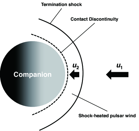
Figure 11.— Schematic view of the Hard X-ray emission from the surface of the companion.

Here we employed a magnetization parameter $\sigma$ for the pulsar wind upstream of the shock, $\sigma=B_{1}^{2}/(4\pi n_{1}u_{1}\gamma_{1},m_{e}c^{2})$ (Kennel & Coroniti, 1984), where $B_{1}$ is the magnetic field just upstream of the shock, $n_{1}$ is the number density of the pulsar wind, $u_{1}$ is the flow velocity defined by $1+u_{1}^{2}=\Gamma_{1}^{2}$ ($\Gamma_{1}$ is the bulk Lorentz factor of the wind upstream of the shock), and $c$ is the light velocity. Assuming that half of the wind energy is carried as Poynting flux ($\sigma=1$), $B_{1}$ amounts to

$$B_{1}=\left(\frac{\sigma}{1+\sigma}\frac{L_{\rm SD}}{R_{\rm orb}^{2}c}\right)^{1/2}=5.5\quad\mbox{G}.$$ (7)

Furthermore, the pulsar wind is compressed at the shock, therefore the downstream magnetic field $B_{2}$ is higher than $B_{1}$. Adopting $B_{2}>5.5$ G as a lower limit, we can constrain the gyration radius of the synchrotron electrons emitting 1 keV X-rays,

$$r_{\rm gyro}=\frac{\gamma_{2}m_{e}c^{2}}{eB}<3.5\times 10^{6}\left(\frac{\epsilon_{\rm X}}{1\mbox{ keV}}\right)^{1/2}\left(\frac{B_{2}}{5.5\mbox{ G}}\right)^{-1}\quad\mbox{cm},\\$$ (8)

where $\epsilon_{\rm X}$ is the synchrotron photon energy. The obtained gyration radius is far smaller than the companion, $r_{\rm comp}\sim 10^{10}$ cm, therefore the shock heated electrons cannot escape from the downstream immediately. In terms of the enegetics, the phase averaged X-ray luminosity of the power-law component was $L_{\rm pow,0.5-10keV}=3.6\times 10^{31}$ erg s^-1 from the spectral fitting. Taking into account the Lorentz boost effect of 1/0.42, and the ratio of the maximum flux against the phase averaged flux of $\sim 3.0$, the intrinsic synchrotron luminosity from the companion becomes $L_{\rm pow,0.5-10keV}^{\prime}=1.1\times 10^{32}$ which is comparable to the bolometric luminosity of the heated hemisphere of the companion, $L_{\rm BB}\sim 1.1\times 10^{32}$ ergs s^-1. This brief estimation also indicates that the heating efficiency should be smaller than 0.5. This result obviously different from the heating efficiency obtained from the phase-resolved SED (see Figure 5) in which an isotropic pulsar wind is assumed. This discrepancy may indicate that the pulsar wind from the central MSP is not isotropic as expected in the crab nebula(Bogovalov & Khangoulyan, 2002). The wind pressure at the companion is then $p_{\rm wind}=L_{\rm SD}/4\pi R_{\rm orb}^{2}c\sim 4.7$ dyn which may be greater than that of the coronal gas ($T=10^{6}$ K, $n_{\rm p}=10^{8}$ cm^-3 for the sun) but much smaller than the photosphere. Therefore the thickness of the emitting region should be not higher than the corona of the companion. On the other hand the radiation length of the relativistic electrons is quite long: $716A/(Z(Z+1)\ln(278/\sqrt{(}Z))\sim 4\times 10^{17}$ cm for the coronal gas of $n_{\rm p}\sim 10^{8}$cm^-3. Therefore these electrons can radiate synchrotron X-rays even in the immediate area of the photosphere.

If the hard X-rays originated in the shocked pulsar wind on the surface of the companion star as is discussed, the composition of the pulsar wind can be constrained based on the downstream flow velocity. Considering the Rankin-Hugoniot relation for magnetized electron-positron plasma for small $\sigma$, we can find the downstream flow velocity as a function of the magnetization parameter $\sigma$ (Kennel & Coroniti, 1984),

$$u_{\rm 2}^{2}=\frac{1+9\sigma}{8},$$ (9)

where $u_{\rm 2}=\Gamma_{\rm 2}\beta_{\rm 2}$. Finally we find the downstream flow velocity, $\beta_{\rm 2}=\sqrt{(1+9\sigma)/(7-9\sigma)}$ in units of the light speed. Note that the equation predicts the lower limit of the shocked pulsar wind, $\beta_{\rm 2}=1/\sqrt{7}\sim 0.38$ at $\sigma=0$. On the other hand, the flow velocity of $\beta_{\rm 2}=0.43\pm 0.15$ from the X-ray light curve indicates that the pulsar wind is already in the particle dominant state, i.e., $\sigma\sim 0.028$, at the surface of the companion, only $1.1\times 10^{11}$ cm apart from the pulsar. Note that the post-shock flow velocity has an inverse-correlation with the inclination angle that affects the resultant magnetization parameter. If we adopt an error range of inclination angle, $50\arcdeg\sim 60\arcdeg$, the magnetization parameter can range from 0.008 (for $i=60\arcdeg$) to 0.1 (for $i=50\arcdeg$). The upper limit of $\sigma<0.1$ is still much smaller than that calculated for the similar system of PSR J1023+0038 reported by Bogdanov et al. (2011), in which a thick post-shock emitting region was assumed. Past theoretical studies claimed that the pulsar wind is highly magnetized at the beginning just around the light cylinder. However, the observed $\sigma$ is far smaller than 1, and this discrepancy has been called the $\sigma$ paradox. Recently Aharonian et al. (2012) reported evidence of particle acceleration just around the pulsar based on gamma-ray pulse analysis of the Crab pulsar. The above argument of $\sigma$ in this work is consistent with their result and may be one of the $\sigma$ parameters measured at the nearest distance from a pulsar. Furthermore this may imply that the old MSPs and the young radio pulsars have the same particle acceleration mechanism.

One of the intriguing features of this object is the double-peak structure in the 2$-$4 keV X-ray light curve. Since the dip is observed only in the softer band (Figure 9), this feature can be interpreted as absorption of soft X-rays. If we accept that the non-thermal X-rays originate in the shocked pulsar wind on the surface of the companion as discussed above, the absorber must be lying around the pulsar, because the dip appears at the optical maximum phase (= the superior conjunction). In addition, the orbital inclination angle $i\sim 55\arcdeg$ requires that the absorber must be extended far from the orbital plane ($\sim 8\times 10^{10}$ cm).

As Ray et al. (2014) claimed, mass accretion on the pulsar seems to continue intermittently, however the argument of the propeller effect rules out a powerful accretion. This is consistent with the lack of a bright disc component in X-ray spectra. In addition to the propeller effects, the measured companion radius is about 1/2 of the Roche lobe, therefore the stellar material cannot overcome the Lagrange point L1 to accrete on the neutron star. To feed mass to the pulsar, explosive ejection faster than $\sim 1000$ km s^-1 may be required for the mass to escape from the gravity potential.

In addition, as inferred from the discussion on the heating efficiency, the pulsar wind may be concentrated on the orbital plane, which would prevent the accretion flow. If the stellar material that is blown away by the equatorial pulsar wind is drifting around the pulsar’s polar regions, and it may accrete from the poloidal direction. On the other hand, the running periodogram shown in Figure 10 indicates that the dip structure related to the second harmonic component is unstable, and appears to have disappeared $\sim 120$ ks from the start time of the observation. To confirm the scenario in which the stellar gas is drifting around the pulsar and accretes intermittently, simultaneous X-ray and radio observations are required.

5. Conclusion

We presented multi-wavelength observations of a newly found black-widow binary system 2FGL J2339.6-0532 covering near-infrared to X-ray regimes. Thanks to a wide wave waveband and long coverage, we successfully obtained a phase-resolved SED that enabled us to constrain the orbital parameters more precisely. The obtained SED seems consistent with past studies, and we calculated an inclination angle of $i\sim 55\arcdeg$, while taking into account the results of recent radio observations. Based on the argument of the propeller-effect argument, the lower limit of the acrretion rate was estimated to be $\dot{m}>1.3\times 10^{16}$ g s^-1, which is about five orders of magnitude larger than that expected from the observed X-ray luminosity. In addition, the estimated orbital parameters imply that the companion’s radius is only 1/2 of the Roche lobe, making it difficult to feed the pulsar continuously. We also obtained an H$\alpha$ image of the vicinity of the target and could not detect any diffuse structure with a 3$\sigma$ detection limit of $<8.7\times 10^{-17}$ erg s^-1 cm^-2 arcsec^-2. We therefore conclude that the target does not have a bow-shock nebula brighter than the H$\alpha$ nebula around PSR B1957+20.

In the X-ray regime, we discovered a steady, soft X-ray component below 1 keV, which seemed to originate from the neutron-star surface, and which showed no evidence of an accretion disc. On the other hand, the hard component above 2 keV showed periodic modulation synchronized with the orbital motion, implying that the hard X-rays originate in the shocked pulsar wind near the companion surface. The observed X-ray luminosity is comparable to the bolometric luminosity of the heated hemisphere of the companion. This means that the heating efficiency should be smaller than 0.5 and the pulsar-wind distribution should be anisotropic. Adopting the above scenario we estimated the magnetization parameter of the pulsar wind $\sigma\sim 0.03$, based on the Rankin$-$Hugoniot relation. This implies that the pulsar wind is already in the particle-dominant state at a distance of 1.1 $\times 10^{11}$ cm from the pulsar. Moreover, we also investigated the time variability of the modulation pattern by using the running periodogram of X-ray light curve, wherein we detected a weakening of the modulation pattern. This may be related to an intermittent weak accretion or an unstable pulsar-wind activity, both of which can cause temporal extinction of the radio-pulse emission.

 

Table 4Summary of optical observations with OISTER

Telescope (Instrument)	Diameter	September 2011							October 2011
		22	23	24	27	28	29	30	1	4	6	7
Pirka telescope (MSI)	160cm		BVRI	BVRI	V	V
Gunma Astronomical Observatory (GIRCS)	150cm					J
MITSuME-Akeno telescope (Tricolor Camera)	50cm	gRI	gRI	gRI	gRI	gRI	gRI	gRI
Kiso Schmidt (2kCCD)	105cm						RH$\alpha$
Kyoto Sangyo University 1.3m telescope (CCD)	130cm					gz
Nayuta telescope (NIC)	200cm	(JHKS)
MITSuME-OAO telescope(Tricolor Camera)	50cm		gRI		gRI	gRI			gRI		gRI	gRI
OAO 188cm telescope (ISLE)	188cm				J
Bisei Spaceguard Center 1m telescope (Optical CCD)	100cm				(r)	(r)
Kanata telescope (HOWPol)	150cm				R	R				V		B
Kagoshima University 1m telescope (IR CCD)	100cm				(J)	(J)			(J)
Murikabushi telescope (Tricolor Camera)	105cm				gRI		gRI	gRI
Kottamia Astronomical Observatory (Optical CCD)	188cm				R	R	R	B
IRSF 1.4m telescope (SIRIUS)	140cm					JHKS	JHKS	JHKS
miniTAO (ANIR)	104cm						RJ	BJ

Note. — The letters on the table describe the observed energy bands. Lower case and upper case characters correspond to the SDSS system and the Johnson$-$Cousins system, respectively. The observations shown in parentheses did not produce usable data due to the weather condition.

References

- Abdo et al. (2010) Abdo, A. A., et al. 2010, ApJS, 188, 405
- Ackermann et al. (2012) Ackermann, M., et al. 2012, ApJ, 753, 83
- Aharonian et al. (2012) Aharonian, F. A., Bogovalov, S. V., & Khangulyan, D. 2012, Nature, 482, 507
- Alpar et al. (1982) Alpar, M. A., Cheng, A. F., Ruderman, M. A., & Shaham, J. 1982, Nature, 300, 728
- Azzam et al. (2014) Azzam, Y. A., Ali, G. B., Elnagahy, F., Ismail, H. A., Haroon, A., Selim, I., & Ahmed-Essam. 2014, ArXiv e-prints
- Becker & Truemper (1997) Becker, W., & Truemper, J. 1997, A&A, 326, 682
- Bogdanov et al. (2011) Bogdanov, S., Archibald, A. M., Hessels, J. W. T., Kaspi, V. M., Lorimer, D., McLaughlin, M. A., Ransom, S. M., & Stairs, I. H. 2011, ApJ, 742, 97
- Bogovalov & Khangoulyan (2002) Bogovalov, S. V., & Khangoulyan, D. V. 2002, Astronomy Letters, 28, 373
- Cardelli et al. (1989) Cardelli, J. A., Clayton, G. C., & Mathis, J. S. 1989, ApJ, 345, 245
- Chatterjee & Cordes (2002) Chatterjee, S., & Cordes, J. M. 2002, ApJ, 575, 407
- Dickey & Lockman (1990) Dickey, J. M., & Lockman, F. J. 1990, ARA&A, 28, 215
- Ferrigno et al. (2014) Ferrigno, C., et al. 2014, A&A, 567, A77
- Fruchter et al. (1988) Fruchter, A. S., Stinebring, D. R., & Taylor, J. H. 1988, Nature, 333, 237
- Fukugita et al. (1996) Fukugita, M., Ichikawa, T., Gunn, J. E., Doi, M., Shimasaku, K., & Schneider, D. P. 1996, AJ, 111, 1748
- Gajjar et al. (2012) Gajjar, V., Joshi, B. C., & Kramer, M. 2012, MNRAS, 424, 1197
- Hester et al. (2002) Hester, J. J., et al. 2002, ApJ, 577, L49
- Itoh et al. (2001) Itoh, N., et al. 2001, Publications of the National Astronomical Observatory of Japan, 6, 41
- Kalberla et al. (2005) Kalberla, P. M. W., Burton, W. B., Hartmann, D., Arnal, E. M., Bajaja, E., Morras, R., & Pöppel, W. G. L. 2005, A&A, 440, 775
- Kargaltsev & Pavlov (2008) Kargaltsev, O., & Pavlov, G. G. 2008, in American Institute of Physics Conference Series, Vol. 983, 40 Years of Pulsars: Millisecond Pulsars, Magnetars and More, ed. C. Bassa, Z. Wang, A. Cumming, & V. M. Kaspi, 171–185
- Kataoka et al. (2012) Kataoka, J., et al. 2012, ApJ, 757, 176
- Kawabata et al. (2008) Kawabata, K. S., et al. 2008, in Society of Photo-Optical Instrumentation Engineers (SPIE) Conference Series, Vol. 7014, Society of Photo-Optical Instrumentation Engineers (SPIE) Conference Series, 70144L
- Kennel & Coroniti (1984) Kennel, C. F., & Coroniti, F. V. 1984, ApJ, 283, 694
- Kong et al. (2012) Kong, A. K. H., et al. 2012, ApJ, 747, L3
- Konishi (2014) Konishi, M. e. a. 2014, accepted for PASJ
- Kotani et al. (2005) Kotani, T., et al. 2005, Nuovo Cimento C Geophysics Space Physics C, 28, 755
- Kulkarni & Hester (1988) Kulkarni, S. R., & Hester, J. J. 1988, Nature, 335, 801
- Landolt (1992) Landolt, A. U. 1992, AJ, 104, 340
- Linares et al. (2014) Linares, M., et al. 2014, MNRAS, 438, 251
- Longair (1994) Longair, M. S. 1994, High energy astrophysics. Vol.2: Stars, the galaxy and the interstellar medium (Cambridge: Cambridge University Press, —c1994, 2nd ed.)
- Motohara et al. (2010) Motohara, K., et al. 2010, in Society of Photo-Optical Instrumentation Engineers (SPIE) Conference Series, Vol. 7735, Society of Photo-Optical Instrumentation Engineers (SPIE) Conference Series, 77353
- Nagayama et al. (2003) Nagayama, T., et al. 2003, in Society of Photo-Optical Instrumentation Engineers (SPIE) Conference Series, Vol. 4841, Instrument Design and Performance for Optical/Infrared Ground-based Telescopes, ed. M. Iye & A. F. M. Moorwood, 459–464
- Papitto et al. (2013) Papitto, A., et al. 2013, Nature, 501, 517
- Pelling et al. (1987) Pelling, R. M., Paciesas, W. S., Peterson, L. E., Makishima, K., Oda, M., Ogawara, Y., & Miyamoto, S. 1987, ApJ, 319, 416
- Ray et al. (2014) Ray, P. S., et al. 2014, in American Astronomical Society Meeting Abstracts, Vol. 223, American Astronomical Society Meeting Abstracts, #140.07
- Roberts (2011) Roberts, M. S. E. 2011, in American Institute of Physics Conference Series, Vol. 1357, American Institute of Physics Conference Series, ed. M. Burgay, N. D’Amico, P. Esposito, A. Pellizzoni, & A. Possenti, 127–130
- Roberts (2013) Roberts, M. S. E. 2013, in IAU Symposium, Vol. 291, IAU Symposium, 127–132
- Romani & Shaw (2011) Romani, R. W., & Shaw, M. S. 2011, ApJ, 743, L26
- Schlafly & Finkbeiner (2011) Schlafly, E. F., & Finkbeiner, D. P. 2011, ApJ, 737, 103
- Skrutskie et al. (2006) Skrutskie, M. F., et al. 2006, AJ, 131, 1163
- Smith et al. (2002) Smith, J. A., et al. 2002, AJ, 123, 2121
- Stella et al. (1986) Stella, L., White, N. E., & Rosner, R. 1986, ApJ, 308, 669
- Takahashi et al. (2009) Takahashi, N., Nishihara, E., & 150cm Telescope Working Group, G. 2009, in Proc. of GAO-ITB Joint Workshop in Astronomy and Science Education, GAO-ITB Joint Workshop in Astronomy and Science Education, 50–60
- Tokunaga & Vacca (2005) Tokunaga, A. T., & Vacca, W. D. 2005, PASP, 117, 421
- Watanabe et al. (2012) Watanabe, M., Takahashi, Y., Sato, M., Watanabe, S., Fukuhara, T., Hamamoto, K., & Ozaki, A. 2012, in Society of Photo-Optical Instrumentation Engineers (SPIE) Conference Series, Vol. 8446, Society of Photo-Optical Instrumentation Engineers (SPIE) Conference Series
- Weisskopf et al. (2000) Weisskopf, M. C., et al. 2000, ApJ, 536, L81
- Yanagisawa et al. (2010) Yanagisawa, K., Kuroda, D., Yoshida, M., Shimizu, Y., Nagayama, S., Toda, H., Ohta, K., & Kawai, N. 2010, in American Institute of Physics Conference Series, Vol. 1279, American Institute of Physics Conference Series, ed. N. Kawai & S. Nagataki, 466–468
- Yoshida (2005) Yoshida, M. 2005, Journal of Korean Astronomical Society, 38, 117