Possible visualization of a superfluid vortex loop attached to an oscillating beam.

Abstract

Visualization using tracer particles is a relatively new tool available for the study of superfluid turbulence and flow, which is applied here to oscillating objects submerged in the liquid. We report observations of a structure seen in videos taken from outside a cryostat filled with superfluid helium at 2 K, which is possibly a vortex loop attached to an oscillator. The feature, which has the shape of an incomplete arch, is visualized due to the presence of solid $H_{2}$ tracer particles and is attached to a beam oscillating at 38 Hz in the liquid. It has been recorded in videos taken at 240 frames per second (FPS), fast enough to take $\sim$ 6 images per period. This makes it possible to follow the structure, and to see that is not rigid. It moves with respect to the oscillator, and its displacement is in phase with the velocity of the moving beam. Analyzing the motion, we come to the conclusion that we may be observing a superfluid vortex attached to the beam and decorated by the hydrogen particles. An alternative model, considering a solid hydrogen filament, has also been analyzed, but the observed phase between the movement of the beam and the filamentary structure is better explained by the superfluid vortex hypothesis.

1 Introduction

In the superfluid phase of liquid Helium, below 2.177 K, the circulation is quantized in units of a flux quantum ($\kappa=h/m_{He}\simeq 10^{-3}cm^{2}/s$ where $m_{He}$ is the mass of a He⁴ atom and $h$ is the Planck constant). The existence of vortices with a single flux quantum was independently proposed by Feynman and Onsager feynman1957superfluidity ; onsager1949suppl and the first measurements showing quantized circulation were made by Vinenvinen1961detection . More recently superfluid vortices have been observed by Bewley et albewley2006 , and this group has developed solid hydrogen tracersbewley2009generation ; bewley2008particles to visualize the flow and has observed many interesting features of vortex physics such as re-connectionsbewley2006 ; bewley2009generation and Kelvin waves fonda2014direct . Visualizations of turbulence generated by counterflow have also been obtained by this techniqueLaMantiaSkrbek2014 ; la2013velocity ; paoletti2008velocity which is becoming a powerful tool in the study of Quantum Turbulenceguo2014visualization .

However, apart from some preliminary workzemma2013part1 , the visualization of flow around objects oscillating in superfluids has not been explored so much, although Vinen and Skrbekvinen2010quantum ; vinen2014quantum have pointed out that tracer imaging of superfluid oscillatory flows with a classical analogue could provide valuable information. We have recently developed a simple system using solid hydrogen particles for visualizing flow around oscillating objects in superfluid heliumzemma2013part1 . In the following we present further observations made using this system which show a behavior which is consistent with the presence of a superfluid vortex half-loop attached to a beam oscillating in liquid helium. The loop is observed to expand and contract and is attached to the beam throughout our observation. To our knowledge, such behavior has not been directly visualized previously, although vortex loops have been observed indirectly through their attachment and detachmentGotoTsubota2008 and discussed theoretically beforeHanninen2009 ; godfrey2001new ; godfrey2000stable . We therefore believe that our observations could shed new light on the problem of superfluid turbulence, in particular on the behavior of vortices attached to a solid boundary with oscillating flow and their stability and pinning.

2 Experimental Details

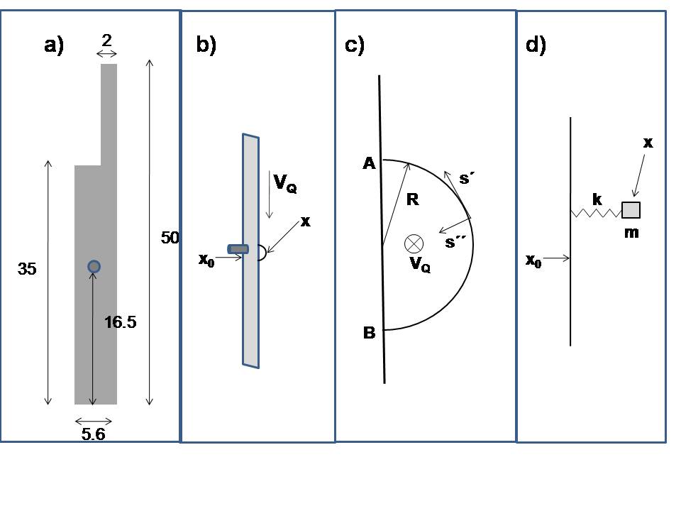
Figure 1: a)Diagram of the vibrating beam, with measurements in millimeters. The position of the driving magnet is shown as a circle in this frontal view of the setup. b) Position of the points $x$ and $x_{0}$ (see text) in the approximate perspective seen in the videos. $V_{Q}$ represents the local superfluid velocity due to the heat load of the cryostat. The driving magnet and its position are shown as a cylinder in perspective. c) Proposed geometry of the vortex loop and definition of some quantities used in the analysis d) Alternative mass-spring model considering a possible hydrogen filament, instead of the loop shown in c).

The experimental arrangement has been described in detail elsewherezemma2013part1 . The system studied consists of a vibrating beam, driven magnetically by using a permanent magnet attached to the beam and a coil fixed to a rigid frame. In this way the beam oscillates with velocity perpendicular to its wide dimension at a frequency of 38 Hz. A sketch of the geometry is found in Fig. 1. Videos are taken with a camera at 240 frames per second (FPS) so the time interval is 4.17 ms between frames and we use this as our time reference to calculate velocities. The helium temperature was 2.07 K throughout the experiment.

A mixture of one part hydrogen to 50 parts helium gas at 500 torr is introduced from room temperature to form the solid hydrogen particles and around a hundred cubic centimeters of gas are injected each time. To illuminate the tracer particles we used a green laser beam. The frozen H₂ particles are not expected to absorb significant energy in the visible CaloryPart . The laser is on the outside of the dewar and the light passes through an optical fiber which ends less than a centimeter away from the oscillating beam, illuminating the particles perpendicular to the line of sight of the camera. The fiber is polished at the end, giving a three dimensional cone of light. Distances in the image are calibrated with respect to the measured dimensions of the small magnet (a cylinder 5mm long and 3 mm in diameter), which is used to drive the oscillator. The size of a pixel corresponds to around 70 microns in the object but the light could be scattered from particles which are smaller than this. It is hard to evaluate the minimum observable dimension, but we estimate our particles to be distributed in size from well below 70 microns to 200 microns.

An important feature of our setup is that we are forced to remove the outer nitrogen Dewar to avoid the blurring of the images produced by the boiling nitrogen. For this reason, the heat load is considerable. We can estimate it by measuring the volume of He evaporated as a function of time and using the known latent heat of evaporation. The heat input $\dot{Q}$ is not constant, but has been roughly measured to lie between 800 and 470 mW. The helium Dewar is 6 cm in diameter, so the calculated counterflow velocity $v_{Q}$ is between 0.085 and 0.05 cm/sec if we assume a uniform heat flow. These numbers are only rough estimates since the geometry is not simple, the heat input comes from radiation through the walls, conduction down the glass walls, etc. On the Dewar there is a flange of 5 cm diameter about 5 cm above the vibrating beam which also complicates the counterflow geometry.

3 Experimental Results

The main observation of the experiment is the existence of a structure formed by the H₂ particles that seems to be attached to the beam and oscillates with it, though not in a rigid fashion. It seems to elongate and contract when the beam oscillates, and has a curved shape, somewhat resembling an incomplete arch. This structure is seen in all videos taken during the experimental run. We show still images in Fig. 2 taken over one complete cycle of the oscillator. The images are amplified close to the maximum resolution and the pixel structure can be clearly seen.

For analysis, we have chosen to follow two points marked in Fig. 2 and Fig. 1 as $x$ and $x_{0}$. Point $x_{0}$ is fixed to the oscillating beam and $x$ is a point on the arch, which is seen to shrink and grow periodically. We have followed $x$ and $x_{0}$ over several cycles of the oscillator, observing the images by eye, and digitizing the positions $x$ and $x_{0}$ by means of a computer. The difference in the position of these two points, which have a sinusoidal motion, is proportional to the length of the arch formed by the decorating particles. We have taken a well defined and easy to follow point for $x_{0}$ instead of the base of the arch, so $x-x_{0}$ has a constant displacement superposed to the periodic component but the sinusoidal variation is proportional to the length of the arch.

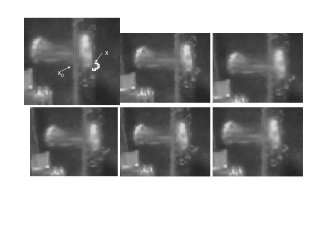
Figure 2: Still images of a video. The six images correspond to successive frames, taken at 4.17 ms intervals and therefore covering a complete cycle of the oscillator whose frequency $\omega_{B}/2\pi=38$Hz. The pixel size can be seen at this magnification.

Digitizing the positions of $x$ and $x_{0}$ we are able to calculate the velocities of the beam and the arch as a function of time (Using the $x_{0}$ positions in successive images and dividing by the known time of 4.17 ms between frames). We can also evaluate the distance $(x-x_{0})$ in each frame. The results are shown on Fig. 3. Open circles correspond to the velocity of the beam and filled circles to the distance $x-x_{0}$. A few cycles are shown, and they include information from three different video sections, all taken the same day but at different times. We have fitted the experimental points with sinusoidal functions by least squares, and the results are shown as lines in the plots. The fits show clearly that the velocity of the beam is in phase with the relative displacement $x-x_{0}$. Bearing in mind that $x-x_{0}$ is proportional to the length of the arch formed by the solid particles, the length of this structure therefore is in phase with the velocity of the beam. We have also evaluated the velocities of $x$ and $x_{0}$ separately, and find that they are around 90 degrees out of phase with each other. Therefore the arch structure is not rigidly attached to the beam, but shows an internal shrinking and growing movement in phase with the velocity.

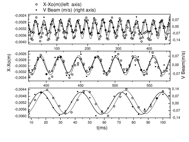
Figure 3: Comparisons of beam velocity $V_{Beam}$ and $x-x_{0}$ for three sections of the videos. Open circles correspond to the velocity of the beam and filled circles to the distance $x-x_{0}$. The dashed and full lines are sinusoidal fits to the data and it can be seen from the graphs that $V_{Beam}$ and $x-x_{0}$ are almost in phase.

The phase difference between velocities and $x-x_{0}$ is shown in a different way in Fig. 4. We show the data in a parametric plot, on the left hand side the velocity of the the beam ($V_{Beam}$) is plotted against a point corresponding to the top of the arch ($Vx$) and it is seen that the plot is almost circular, as corresponds to a parametric representation of two sinusoidal functions with a 90 degree phase difference, while on the right a plot of $x-x_{0}$ against $V_{Beam}$ shows a very elongated ellipse at a 45 degree angle, as would be seen for two sinusoidal functions that are almost in phase.

Although we only show a few periods, videos are longer than this, and the motion of the arch was observed to remain basically unchanged throughout the whole experimental run. The video camera was not always on, but the oscillation of the beam was not changed for 13 minutes. During this time we filmed ten sections of video at 240 and 480 frames per second, and in all of them we see the loop, with similar behavior. The sections shown are representative of the first and last parts filmed, at 240 FPS. We have not included data for the 480 FPS because the resolution and lighting are not good enough for measuring quantitatively, although the images show movement of the loop that is compatible with that seen at 240 FPS. Several experiments with the same setup were performed, but the structure seen here was seen in only in this particular run when the videos were analyzed in detail later. It seems therefore that the formation of a loop is not a reproducible feature, but depends on several uncontrolled factors as is expected in turbulent regimes.

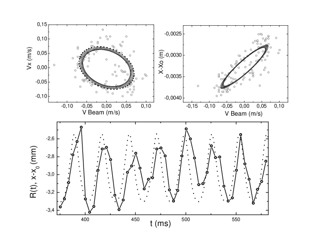
Figure 4: Upper panel: Parametric plots of $Vx$ vs $V_{Beam}$ (left), and $x-x_{0}$ vs $V_{Beam}$ (right). Open circles: experimental points, lines: sinusoidal fits to the data, equivalent to the full and dotted lines shown in Fig. 3. The almost circular plot on the left indicates that the corresponding sinusoidal motions are 90 degrees out of phase, while the highly tilted ellipse at the right implies that the oscillations are almost in phase. Lower panel: Fit of $x-x_{0}\propto R(t)$ using Eq. 3 and fitting parameters $A=0.37$ , $B=0.001$. Lines and open circles correspond to the measured $x-x_{0}$ and the fit is shown in dotted lines. The good agreement indicates that the vortex loop model gives an adequate description of the observations.

4 Discussion

We have come to the conclusion that the behavior observed is consistent with the motion expected from a vortex half-loop pinned to the beam. This appears to cover the main facts, although other possibilities have also been considered. We use for our analysis the relationship obtained by Schwarzschwarz1985 for a stable vortex loop. According to hisschwarz1985 Eq. 20 a vortex loop of radius $R_{0}$ will not shrink or grow if it moves with a velocity $v_{s}$ with respect to the superfluid:

$$v_{s}=\frac{\kappa}{4\pi R_{0}}\ln\left[\frac{8R_{0}}{e^{1/4}a_{0}}\right]$$ (1)

with $a_{0}\approx 1.3\times 10^{-8}$ cm an adjustable parameter roughly equivalent to the size of the vortex core. Conversely, if the loop is fixed in position, a flow of the superfluid with velocity $v_{s}$ maintains a stable radius, if the sign of the velocity and the vorticity of the loop are in the right orientation. Section IV A of Ref. schwarz1985 is also relevant to our situation, since it discusses a bent vortex loop pinned at two points and his Fig. 29 shows the shape calculated for different values of superfluid velocity. In our case, using Eq. 1 and an average curvature radius of 0.3 mm the velocity $v_{s}$ for a stable half loop would be 0.027 cm/s. The estimate for the average counterflow velocity $V_{Q}$ is a factor between 2 to 3 times greater than $v_{s}$. However the flow due to $V_{Q}$ close to the beam would probably be lower than $V_{Q}$ itself due to the obstacles present. If we assume that $V_{Q}$ along the beam is modulated by the periodic motion of the beam, we could explain the stretching and contraction of the arch attached to the oscillating beam. The modulation due to the beam $V_{Beam}$ and the counterflow velocity would add to produce a time dependent velocity

$$v_{Osc}(t)=A\cdot V_{Q}+B\cdot V_{Beam}\sin(\omega t)$$ (2)

where $A$ and $B$ are adjustable parameters, $V_{Beam}$ is the measured velocity of the beam, and $\omega$ the oscillating frequency.

From Eq. 1 we can obtain an approximate expression for the radius of the loop due to the time dependent velocity

$$R(t)=\frac{\kappa}{4\pi(A\cdot V_{Q}+B\cdot V_{Beam}\sin(\omega t))}\cdot C$$ (3)

Where $R_{0}=\frac{\kappa}{4\pi A\cdot V_{Q}}\cdot C\approx 0.3$ mm would be the stable radius if $V_{Q}$ has no modulation, and we have not considered significant the modulation of the logarithmic term, including it as a constant $C=\ln\left[\frac{8R_{0}}{e^{1/4}a_{0}}\right]$. We have fitted $(x-x_{0})\sim R(t)$ to the expression given by Eq. 3 and we show the results in the bottom panel of Fig. 4. The adjustable parameters used are $A=0.37$ and $B=0.001$, and a shift has been introduced to compensate for the arbitrary origin when choosing $x_{0}$. In this case we have used the lower value of $V_{Q}=0.05$ cm/s. The fit is quite good, and although it is not a least squares fit and the parameters were chosen by hand, the equation is capable of reproducing the observations.

A second possibility is that the structure seen is not a vortex loop, but a filament of solid hydrogen, as has been observed by Gordon et algordon2007filament ; gordon2009catalysis . We could model a solid filament as a mass attached to a spring, as is shown in Fig. 1 d). The movement of the attaching point $x_{0}$ would move the mass at $x$ as a forced harmonic oscillator

$$m\ddot{x}+\gamma\dot{x}+k(x-x_{0})=0$$ (4)

the well known solution for this equation is harmonic motion, with a phase difference $\phi$ between $x_{0}$ and $x$. Our observed phase difference is of around 90 degrees, between these quantities, which would be the case only if the driving frequency $\omega_{B}/2\pi$ of 38 Hz were accidentally close to the resonance frequency of the filament $\omega_{f}=\sqrt{k/m}$. It is highly unlikely that $\omega_{f}$ is the same as the frequency of the beam $\omega_{B}$, and it could be expected that $\phi$ would either be zero (if $\omega_{f}>>\omega_{B}$) or 180 degrees (if $\omega_{f}<<\omega_{B}$). A third possibility is that the oscillating filament could be overdamped by the influence of the normal component, but in this case $x$ would follow the fluid, which in the reference frame of the laboratory, moves 180 degrees out of fase with the point $x_{0}$ belonging to the beam. In fact, our observation could be a combination of a hydrogen filament and part of a vortex loop, attached to the end of the filament and a point in the beam. The filament shown in Fig. 3 of Ref. gordon2009catalysis shows movement in the normal fluid, but to have the phase observed here some form of vortex section, closing the loop and with movement given by Eq. 3 seems to be necessary to explain the observed behavior.

For further analysis, the local approximation could also be used, and in this approach the dynamics of a quantized vortex is described by the equation proposed by Schwarzschwarz1988three

$$\frac{d\textbf{s}}{dt}=\beta\textbf{s}^{\prime}\times\textbf{s}^{\prime\prime}+\textbf{v}_{s}+\alpha\textbf{s}^{\prime}\times(\textbf{v}_{n}-\textbf{v}_{s}-\beta\textbf{s}^{\prime}\times\textbf{s}^{\prime\prime})$$ (5)

here s is a point on the core of a vortex loop, $\beta$, $\alpha$ the coefficient of mutual friction, $\textbf{v}_{n}$ and $\textbf{v}_{s}$ the velocities of the normal and superfluid fractions, $\textbf{s}^{\prime}$ is the tangent to the vortex core, $\textbf{s}^{\prime\prime}$ the principal radius. The proposed structure of the vortex half-loop and the definition of the vector quantities $\textbf{s}^{\prime}$ and $\textbf{s}^{\prime\prime}$ in Eq. 5 are shown in Fig. 1. We can assume that the vibrating beam pushes both the normal fluid and the superfluid together, as well as modulating $V_{Q}$ as described above, so we have

$$\textbf{v}_{n}\cdot\hat{\textbf{r}}=\textbf{v}_{s}\cdot\hat{\textbf{r}}=v_{1}\sin\omega t\cdot\cos\varphi$$ (6)

with $\varphi$ the angle between the local velocity and the vortex. Then Eq. 5 implies

$$\frac{dR}{dt}=D\cdot v_{1}\sin\omega t\cdot\cos\varphi-\frac{\alpha\beta}{R}$$ (7)

The equation is local, so that $\frac{dR}{dt}$ changes over the circumference with $\cos\varphi$. It also changes the shape of the half loop, depending on the relative orientation of loop and velocity, but we can get an approximate value for the average radius $\left\langle R\right\rangle$ neglecting the second term with respect to the first and integrating in time and over $\varphi$

$$\left\langle R\right\rangle=R_{0}-D\frac{v_{1}}{\omega}\cos\omega t.$$ (8)

with $D$ a parameter taking into account the angular integration over $\varphi$. We do not have enough resolution to detect the changes of shape implied by Eq. 8, but it would appear that the effect is smaller than that of Eq. 3. Furthermore it gives motion with a phase that is at 90 degrees from the velocity of the beam, instead of the in phase motion observed.

In fact, Eq. 3 can be taken as a quasi static non local solution including a modulation of $V_{Q}$, and Eq. 8 as a local time dependent correction due to the presence of $v_{1}$ whose importance is given by the parameter $D$. The good fit obtained with Eq. 3, seen in Fig. 4 seems to indicate that the effect of the correction of Eq. 8 is not very large, although it could be responsible for the fact that in the measurements $x-x_{0}$ and $V_{Beam}$ are not always in phase. In fact, seen over many cycles, there are small irregularities in the motion, where the structure seems to stretch more or less. However, the overall stability is preserved, as stated earlier, over at least the 13 minutes where we have partial observations. Since the frequency is 38 Hz, the number of cycles over which the stretching and shrinking is repeated is of order $3\times 10^{4}$.

In conclusion, we have observed, by decoration with solid $H_{2}$ tracers, a structure which moves attached to a vibrating beam. From an analysis of possible models for the observed motion, we conclude that it behaves as expected for a vortex half-loop attached to the oscillator. This accounts for the phase relationship between position and velocity, and we obtain a good fit between the model and the video images, while an alternative explanation postulating a hydrogen filament requires an unlikely coincidence between the driving frequency and the natural frequency of the hydrogen filament. A third model, considering that the motion is due to the drag of the normal component on an over damped filament, would also produce a phase difference that is not the one observed.

- (1) Feynman R P 1957 Reviews of modern physics 29 205–212
- (2) Onsager L 1949 Nuovo cimento 6 249–250
- (3) Vinen W 1961 Proceedings of the Royal Society of London. Series A. Mathematical and Physical Sciences 260 218–236
- (4) Bewley G, Lathrop D and Sreenivasan K 2006 Nature 441 588–588
- (5) Bewley G 2009 Cryogenics 49 549–553
- (6) Bewley G, Sreenivasan K and Lathrop D 2008 Experiments in Fluids 44 887–896
- (7) Fonda E, Meichle D P, Ouellette N T, Hormoz S and Lathrop D P 2014 Proceedings of the National Academy of Sciences 111 4707–4710
- (8) La Mantia M and Skrbek L 2014 EPL (Europhysics Letters) 105 46002
- (9) La Mantia M, Duda D, Rotter M and Skrbek L 2013 Procedia IUTAM 9 79–85
- (10) Paoletti M, Fisher M, Sreenivasan K and Lathrop D 2008 Physical review letters 101 154501
- (11) Guo W, La Mantia M, Lathrop D P and Van Sciver S W 2014 Proceedings of the National Academy of Sciences 111 4653–4658
- (12) Zemma E and Luzuriaga J 2013 Journal of Low Temperature Physics 173 71–79
- (13) Vinen W 2010 Journal of Low Temperature Physics 161 419–444
- (14) Vinen W F and Skrbek L 2014 Proceedings of the National Academy of Sciences 111 4699–4706
- (15) Goto R, Fujiyama S, Yano H, Nago Y, Hashimoto N, Obara K, Ishikawa O, Tsubota M and Hata T 2008 Phys. Rev. Lett. 100(4) 045301
- (16) Hänninen R, Tsubota M and Vinen W F 2007 Phys. Rev. B 75(6) 064502
- (17) Godfrey S and Samuels D 2001 Journal of low temperature physics 125 69–85
- (18) Godfrey S P and Samuels D C 2000 Physical Review B 61 4190
- (19) Penney R and Hunt T K 1968 Phys. Rev. 169(1) 228–228
- (20) Schwarz K 1985 Physical Review B 31 5782
- (21) Gordon E B, Nishida R, Nomura R and Okuda Y 2007 JETP Letters 85 581–584
- (22) Gordon E and Okuda Y 2009 Low Temperature Physics 35 209–213
- (23) Schwarz K 1988 Physical Review B 38 2398