Non-Markovianity and memory effects in quantum open systems
Abstract
Although a number of measures for quantum non-Markovianity have been proposed recently, it is still an open question whether these measures directly characterize the memory effect of the environment, i.e., the dependence of a quantum state on its past in a time evolution. In this paper, we present a criterion and propose a measure for non-Markovianity with clear physical interpretations of the memory effect. The non-Markovianity is defined by the inequality in terms of memoryless dynamical map introduced in this paper. This definition is conceptually distinct from that based on divisibility used by Rivas et al (Phys. Rev. Lett 105, 050403 (2010)), whose violation is manifested by non-complete positivity of the dynamical map. We demonstrate via a typical quantum process that without Markovian approximation, nonzero memory effects (non-Markovianity) always exist even if the non-Markovianity is zero by the other non-Marovianity measures.
I Introduction
The Markov approximation is widely used to study open quantum systems, leading to a reduced dynamics where the future state of the system depends only on its present state. Mathematically, a quantum Markovian process can be described by a master equation in the Lindblad form, or equivalently by completely positive divisible mapsBreuerbook ; Rivas . Strong-coupling, finite-size environments or small time scales might lead to the failure of the Markov approximation. Memory effects then become important, and the dynamics in this case is said to be non-Markovian. It was found that the non-Markovianity is usually associated with the occurrence of revivals, non-exponential relaxation, or negative decay rates in the dynamics. In recent years, the features of the non-Markovian quantum process attracted attention in both theoretical and experimental studies Chruscinski ; Jing ; Fanchini ; Xu ; Madsen ; Liu ; Zhang ; Chin ; Huelga ; Deffner ; Kennes ; Tahara ; Cerrillo ; Shabani . A number of quantitative measures have been proposed to quantify non-Markovianity, such as the quantum channels Wolf , the non-monotonic behaviors of distinguishability Breuer ; Laine ; Vasile ; Liuj , entanglement Rivas2 , Fisher informationLu , correlation Luo , the volume of states Lorenzo , capacity Bylicka , the breakdown of divisibility Rivas2 ; Hou , the negative fidelity difference Rajagopal , the nonzero quantum discord Alipour , the negative decay rates Hall , and the notion of non-Markovian degree Chruscinski2014 .
Among them, the measure defined by Breuer, Laine and Piilo Breuer is closely related to the memory effect: Non-Markovianity in this measure manifests itself as a reverse flow of information from the environment to the system. This back-flow of information might be a sufficient condition for the memory effects. It is worth addressing that the essence of the non-Markovianity is whether the future state depends on its past state or not. To that extent, there are no straightforward witnesses for non-Markovianity to date, although a great deal of effort has been made to understand the non-Markovianity. The reason that previous measures Wolf ; Breuer ; Laine ; Vasile ; Liuj ; Rivas2 ; Lu ; Luo ; Lorenzo ; Bylicka ; Hou ; Rajagopal ; Alipour ; Hall ; Chruscinski2014 might not capture directly the memory effect is the physics behind the definitions. The measure in Ref.Wolf investigates whether a quantum channel is consistent with a Markovian evolution. The measure proposed by Rivas, Huelga, and Plenio uses divisibility as a measure of non-Markovianity which characterizes the noncomplete positivity of the dynamical map Rivas2 . The noncomplete positivity is improved in Hou , but it still could not capture the memory effects. The other non-Markovianity measures in Refs. Breuer ; Laine ; Vasile ; Liuj ; Rivas2 ; Lu ; Luo ; Lorenzo ; Bylicka ; Rajagopal ; Alipour ; Hall ; Chruscinski2014 are based on features different from those mentioned before, however these features are intrinsically related to the non-complete positivity of dynamical maps in quantum evolutions. Therefore, the measures so far do not directly reflect how the future state of a quantum system depends on its past. This stimulates us to consider the following questions: How do we directly quantify this memory effect? Is non-exponential but monotonic relaxation a Markovian process or a non-Markovian one? What is the essential difference between a time-dependent Markovian equation and a non-Markovian time-local equation? In this paper, we will try to study these questions by quantifying the non-Markovianity directly based on the memory effect.
Generally speaking, the conventional dynamical map is ambiguous unless the initial time of the evolution is fixed. We define (for details, see below) as the dynamical map transferring state from to , where (arbitrary) is the initial time of the evolution. The initial time means the state of the whole system is in a product state at this point in time. We will show the difference between and in latter discussions. By this definition, is always completely positive (CP) and trace preserving (TP) for arbitrary in quantum processes. The Markovian divisibility condition can be expressed in terms of dynamical map as because the dynamical map in a Markovian process does not depend on the initial time of evolution. In the non-Markovian regime, the divisible condition in terms of is conceptually distinct from the conventional one since is no longer a dynamical map connecting and . Instead, and correspond to two evolutions with different initial times in a quantum process. Our main result is that the non-Markovianity in terms of is manifested by inequality which has a physical explanation that the evolution depends on its history. This is distinct from the non-Markovianity measure defined via completely positive divisibility discussed in Refs.Rivas2 ; Hou ; Chruscinski2014 for the dynamical map.
With those notations, the non-Markovianity is then defined as the maximum distance between and over and . It reflects the degree of memory effects in a quantum process. We calculate the non-Markovianity of a typical quantum process where a qubit decays into vacuum with different environmental spectra. The results show that a non-zero memory effect (non-Markovianity) always exists in this process, even if it is Markovian by the previous measures. Our measure applies to a quantum process that can describe evolutions starting from an arbitrary time , rather than an evolution with a fixed initial time.
The paper is organized as follows. In Sec.II, we review the dynamics of open quantum systems and the concept of universal dynamical map. In Sec.III, we define two types of dynamical maps, and , with different physical meanings. The non-Markovian criterion and measure is introduced in Sec.IV in terms of . In Sec.V, we calculated and discuss the non-Markovianity of an exactly solvable model. Finally, we summarize in Sec.VI.
II dynamics of open quantum systems
A natural way to model an open quantum system is to regard it as arising from an interaction between the system and the environment (denoted by and ), which together form a closed quantum system. The reduced density matrix for the system is obtained by tracing out the environmental degrees of freedom, i.e., . The total Hamiltonian for the system and the environment can be written as,
| (1) |
where , and represents the Hamiltonian of the system, the environment and the coupling, respectively. Consider the total density matrix at , , which undergoes a unitary evolution. The system density matrix at () is given by
| (2) |
where . In a general case where the total Hamiltonian is time-dependent, can be expressed as with the chronological operator. Eq.(2) can be understood as a map connecting and , namely,
| (3) |
In general, such a map depends not only on the total evolution operator and properties of the environment, but also on the system state because may contain correlations between the system and the environment Rivas . Given a fixed of the environment and the correlations between and , not all are allowed due to the positivity requirement of . For example, if the correlation is non-zero, can not be a pure state Rivas . Moreover, it is well known that may not be CP.
A dynamical map which is independent of the state it acts upon is called a universal dynamical map (UDM). It describes a plausible evolution for any statesRivas . Being TP and CP, a UDM can be expressed in the Kraus representation,
| (4) | |||||
where . It turns out that a dynamical map is a UDM if and only if it is induced from the initial condition where is fixed (independent of the system state) for arbitrary Rivas .
Notice that in a Markovian or non-Markovian quantum process, an evolution could start not only at , but also at the other times, say, () where we refer to as the initial time of the evolution. Starting at implies that the total state of the system and the environment satisfies conditions at . In this paper, we focus on quantum processes where the evolutions start with an initial product state of the system and the environment, i.e., where is fixed and is arbitrary. In other words, we study models describing a system in arbitrary states interacting with the environment in a fixed initial state. This consideration is reasonable as it means that the system and the environment are independent at the beginning and then start their evolution. Typically, is stationary under a time-independent environment Hamiltonian , i.e., for any . For example, the equilibrium state or the vacuum state of the environment is often chosen as an initial environment state to study the reduced system dynamics. For a general (nonstationary) initial environment state, it can be given by
| (5) |
where we have assumed that before an evolution starts, initial state of the environment undergoes free evolution driven by [].
With the factorized initial state, the dynamical maps starting from any time are UDMs characterized by the fixed initial environment state and the global unitary evolution (total Hamiltonian), rather than the initial system state. Consequently, the quantum processes are supposed to have fixed non-Markovianity as a function of and , regardless of the system states. On the other hand, the quantum process is universal because it can describe the evolution of any initial system state. In the case of and , which is the usual assumption used to investigate the dynamics of an open quantum system, we expect a time-independent value of non-Markovianity of the quantum process. Otherwise, the non-Markovianity may depend on the time interval that we are interested in since the quantum process is not time- homogenous.
III Dynamical maps with and without memory
The reduced dynamics of an open quantum system can be represented by dynamical maps. In particular, quantum non-Markovian behaviors are often discussed with the help of the dynamical map that transforms the state from to However, in general the physical meaning and properties of are not clear unless we know the total density matrix , or, from another point of view, the initial time of the evolution. For instance, let ; when the evolution starts at , which means , the map is a UDM. In contrast, when the evolution starts at a fixed time , the total density matrix at is , and then can be understood as an intermediate map that is in general not a UDM. Obviously, has different meanings and properties for different initial times of evolution. This is crucial for understanding non-Markovian characters since it tells us that the evolution of the system after [determined by ] is related to its history (from to ). To clarify this point, we introduce two types of dynamical maps denoted by and , respectively. We will describe the two dynamical maps in the following.
III.1 Type I: dynamical map with memory
is defined as the quantum dynamical map transferring the state from to when the evolution starts at a prescribed time (), i.e., . When , can be understood as an continuous map. The physical meaning of can be expressed as
| (6) | |||||
where and defined by Eq.(5). is in general not a product state with fixed environment state due to the system-environment interaction, this means is not a UDM in general. The history of the system from to is encoded in . We will refer to this type of map as dynamical map with memory. This interpretation of the dynamical map is frequently used to investigate the non-Markovinity of quantum dynamics.
In particular, when the starting time of the map is the initial time of the evolution, i.e., , is a UDM represented by,
| (7) | |||||
which can map any system state to another physical state.
III.2 Type II: memoryless dynamical map
Next, we define as the quantum dynamical map transferring the quantum system from state to , where is the initial time of the evolution, i.e., . The initial total state is with fixed defined by Eq.(5) and arbitrary . Then, can be expressed as,
| (8) | |||||
is always a UDM in contrast to . As is independent of the system’s history, the map is memoryless. We remind the reader that in a quantum process, and () correspond to different evolutions.
In particular, when the total Hamiltonian is time-independent and the initial environmental state is stationary, we have
| (9) | |||||
One can easily observe that the map is time-homogeneous, i.e., . This feature was discussed by Chruściński and Kossakowski in Ref. Chruscinski , leading to the existence of an initial time in a non-Markovian time-local master equation,
| (10) |
such that . Eq.(10) provide a full description of the quantum non-Markovian process where evolutions starting at any time are included. The initial time is usually ignored in literature provided that one only considers evolutions starting from , leading to which may have the same form of a time-dependent Markovian equation with non-negative decay rates. However, the existence of the initial time is the essential feature of a non-Markovian time-local equation compared with a time-dependent Markovian equation. It provides an evident signature of the memory effect since the dynamical map sending to relies on the initial time (), i.e., the history of the system, while in a time-dependent Markovian equation, is uniquely defined.
When is the initial time of the evolution , we have by definition. The key difference between the two types of dynamical maps and exists when is not the initial time. When , in general since is in general not with fixed . Given a quantum process characterized by the total Hamiltonian and the initial environment state, the map is well-defined and straightforward to calculate compared with . With these notations, the non-Markovianity can be defined by the use of the memoryless dynamical map in the following section.
IV Non-Markovianity based on memory effects
In this section, we give a condition as well as a measure for quantum non-Markovinity quantifying the degree of the memory effect. Let us start from the quantum Markov process. A quantum process is called Markovian if the corresponding dynamical map, which we denote by in this paper, is divisible. i.e.,
| (11) |
where all maps are UDMs (CP and TP) defining a one-parameter semigroups. Equivalently, the quantum Markovian process can be described by a master equation in Lindblad form, Lindblad
| (12) | |||||
with . The evolution of the system is given by where . More generally, when the generator varies with time due to the change of external conditions, the process is called time-dependent Markovian which satisfies a time-dependent master equation in Lindblad form,
| (13) | |||||
with . The dynamical map becomes which is inhomogeneous but still a UDM, and the evolution of the system can be described by . The divisibility condition can then be written as
| (14) |
where each dynamical map is a UDM. We will discuss in the following the time-dependent Markovian process without loss of generality.
In a quantum (time-dependent) Markovian process, the dynamical map transferring to is uniquely given by the UDM regardless of the system’s history before . We remark that the map is a UDM if and only if it is induced from a product state, i.e.
| (15) | |||||
where is a fixed state and is arbitrary. The evolution of the system at any time in a (time-dependent) Markovian process can be understood by examining Eq.(15). It is interpreted as the collisional model as reviewed in Ref.RivasR . Particularly, when the total Hamiltonian and the initial environmental state are time-independent, the map can be understood as
| (16) | |||||
which depends only on the difference , corresponding to a homogeneous Markovian process described by Eq.(11) or Eq.(12).
In a real Markovian quantum process, the total state of the system and the environment may not remain perfectly factorized as in Eq.(15), and is not a UDM in general. From this point of view, the exact dynamics of an open quantum system is never perfectly Markovian Rivas . However, if with fixed (independent of the system state) where the correlation between the system and environment does not affect so much the system’s dynamics, a Markovian model is still a good approximate description.
An important observation is that the evolution from any time in a quantum (time-dependent) Markovian process can be interpreted as Eq.(15) where the total state remains a product state and the environmental state is fixed for arbitrary . No matter the initial time of an evolution is or (or any time before ), the dynamical map transferring to is always given by . Therefore, the Markovian dynamical map can be interpreted as both and according to our definitions in Sec.III, i.e.,
| (17) |
for any . Consequently, in a Markovian process, the divisibility condition Eq.(14) can be expressed both in terms of and , respectively,
| (18) | |||
| (19) |
Any violation of the above two divisibility conditions will be a manifestation of non-Markovianity. Interestingly, the violations of Eq.(18) and Eq.(19) have different physical interpretations which can lead to different criteria and measures for quantum non-Markovianity. The violation of Eq. (18) is usually manifested by the non-complete positivity of the intermediate map in evolutions starting at , which is the ultimate reason behind the behaviors of different quantities (such as the trace distance, entanglement, correlation and so on) in Refs.Breuer ; Laine ; Vasile ; Liuj ; Rivas2 ; Lu ; Luo ; Lorenzo ; Bylicka ; Rajagopal ; Alipour . The violation itself also accounts for the measures in Refs. Rivas2 ; Hou ; Hall ; Chruscinski2014 . In contrast, the dynamical maps in Eq.(19) are all UDMs, i.e., CP and TP, and the violation of the second divisibility condition Eq.(19) is manifested by the inequality
| (20) |
A quantum process is non-Markovian if there exists such that the inequality Eq.(20) holds. This criterion is conceptually different from others. It has a clear physical interpretation in terms of memory effects, which we will explain in the following.
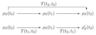
Consider the left-hand and right-hand sides of Eq.(20) acting on an arbitrary state , respectively, as shown in Fig.1. On the left-hand side of Eq.(20), is mapped to by in evolution A, while on the right-hand side, is firstly mapped to by in evolution B. Then, as an initial state, is mapped to by in evolution C, which starts at with . If , there exists such that . We remind the reader that in both evolutions A and C, the system state at is , but with different histories: in evolution A, has a history from to which is taken into account by . Nevertheless, in evolution C, serves as an initial state without any history before . Therefore, the fact that is a direct manifestation of the memory effect where the future evolution (after ) of the system depends on its history (from to ). This is the fundamental property of non-Markovianity. If provided , then for any , we say that the future state of the system depends only on its present state, i.e., the process is Markovian.
From the environment side, the physics of Eq.(20) can be interpreted as follows. At the end of evolution B, the total state of the system and the environment is . Then, at the beginning of evolution C, the environment is initialized by such that , where is the initial environmental state at defined in Eq.(5). The terminology initialize means the system information acquired by the environment in the time interval is erased at time . Note that the initialization never happens in evolution A. After , if the future system states in evolutions A and B are different, that means the environment ”remembers” the history of the system [encoded in the ] and the future system is affected by this kind of memory.
We define the non-Markovianity as the maximum distance between and over all and (We may investigate a quantum process with a fixed ),
| (21) |
Here denotes some distance measurement between the two quantum dynamical maps and . (Here the concatenation of the two UDMs and is also a UDM). This definition allows us to quantify non-Markovianity directly through dynamical maps without optimization of quantum states Breuer . It can be understood as the maximal deviation of the divisibility condition Eq.(19). When , a quantum process loses its memory effects and becomes Markovian.
To choose a distance measure between two dynamical maps for our non-Markovianity, we remark that a dynamical map is isomorphic to its Choi-Jamiółkowski matrix Choi ; Jamiolkowski defined as . Here is the identity map, and is a maximally entangled state of the system and an ancillary system. The Choi-Jamiółkowski matrix has been used in Ref.Rivas2 to quantify the non-complete positivity and measure the non-Markovianity. Meanwhile, it is often used for measuring the fidelity or distance between two quantum channels (typically a general channel and a unitary one) Gilchrist ; Raginsky ; WATROUS ; Johnston . Here we can easily measure the distance between two dynamical maps and through the trace distance of their Choi-Jamiółkowski matrices, i.e.,
| (22) |
where is the trace norm of an operator . The good properties of the trace distance can be taken advantage of for measuring the distance of dynamical maps Gilchrist . Finally, from Eq.(21) and Eq.(22), the non-Markovianity is given by
| (23) |
which naturally gives a finite value of non-Markovianity satisfying for any quantum process without normalization.
Given a theoretically described quantum process, the dynamical map is always CP and describes a physically plausible evolution. The determination of (or its Choi-Jamiółkowski matrix) is straightforward as long as the evolution starting from is known, regardless of how the process is described. In experiment, () could be determined through quantum process tomography (quantum state tomography) Nielsen . When the complete information about is unavailable, can be used as a sufficient condition of non-Markovianity which is easy to verify both theoretically and experimentally. Moreover, for any observable , is sufficient for non-Markovianity.
V Example
In this section, we illustrate how our measure can be calculated with a typical quantum process. The model describes a two-level system (denoted by S) decaying into its environment (denoted by E), which is initially in the vacuum state. This model is exactly solvable and extensively discussed to study the non-Markovian behaviors. The total time-independent Hamiltonian is written as
| (24) |
where , are the free Hamiltonians of S and E, and denotes the coupling between the qubit and the environmental modes. In the case that where is arbitrary and is the vacuum state, the evolution starting at in the interaction picture) can be expressed in terms of dynamical map as
| (27) | |||||
where the function satisfies
| (28) |
with the correlation function Breuerbook .
Since the total Hamiltonian is time-independent and the initial environmental state is invariant under the total Hamiltonian, the map is time homogeneous according to the discussion in Sec.2, i.e., . Thus, the evolution starting at () can be easily obtained as
| (29) |
Alternatively, the evoltuion starting at can be described by the following master equation
| (30) | |||||
where and . According to Eq.(30), is given by . We stress here that Eq.(30) can only describe evolutions starting at rather than an arbitrary time . Instead, the master equation describing the full quantum process contains the initial time Chruscinski ,
| (31) | |||||
such that which is consistent with Eq.(29).
Assume the spectral density of the bath are Lorentzian and of the form where is connected to the environment correlation time by and determines the time scale of the system by . The solution of Eq.(28) is given by with Breuerbook . Since is real, we have in Eq.(31). Typically, the exact dynamics of an open quantum system is not Markovian as discussed above. In this example, when the environment correlation time is much smaller than the system characteristic time , i.e., , a Markovian model can be a good approximation Breuerbook ; Breuerrev . Thus the non-Markovianity of this quantum process can be characterized by the parameter . When , the process can be described by Eq.(31) with . Interestingly, when we only consider evolutions starting at 0, Eq.(31) reduces to Eq.(30) which has the form of a time-dependent Markovian equation Eq.(13) ( but with different meanings because is undefined in Eq.(30) for ). Therefore, the process with is called Markovian by previously proposed measures that use evolutions starting at a fixed time. It seems counter-intuitive that even though is comparable to , for example, , the process is still called Markovian. Also, other intuitively non-Markovian models might be called Markovian by previous measures Apollaro . In contrast, we will show that non-zero non-Markovianity (memory effects) always exist in this exact model, even for . In addition, the non-Markovinianity tends to zero as . Thus our measure reflects how valid the Born-Markov approximation is in this model.
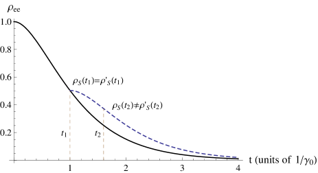
We first demonstrate that when , the evolution in the quantum process depends on its history proving the process is non-Markovian. Consider that the first evolution starts at where the system is initially in its excited state, i.e., . Then, the system density matrix at is given by . Now we assume the second evolution starts at with initial state such that . At a further time , we have in the first evolution and in the second evolution. The result is visualized in Fig.2 by evaluating the evolutions of the excited-state population with . From the fact that , we conclude that the future states (after ) of the system are relevant to its history (from to ) in the process. The exited-state population decays monotonically and non-exponentially in this case. Although the decay rate is non-negative and the revival of does not occur, the environment is affected by the system’s history and then has an influence on the future evolution of the system. Thus the dashed line and the solid line in Fig.2 do not overlap. This phenomenon never happens in a (time-dependent) Markovian process described by Eq. (13), where the dynamical map transferring to is uniquely given by regardless of the initial time.
The non-Markovianity for this quantum process is calculated as follows. From Eq.(27) and Eq.(29), we obtain the Choi-Jamiółkowski matrix of
| (32) | |||||
| (37) |
where . Similarly, the Choi-Jamiółkowski matrix of is
| (43) |
where and . According to Eq.(23), the non-Markovnianity in the case of the Lorentz spectrum is
| (44) | |||||
where , and . Notice that this result has been simplified by the fact that is real.
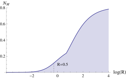
We calculate the non-Markovianity by numerically optimizing the two time differences and . is plotted as a function of in Fig.3 where varies from to . The result demonstrates that the non-Markoviaity is non-zero for all . It monotonically decreases with and tends to as . It is observed that when , the non-Markovianity is already very small (), implying that the quantum process is approaching Markovian and almost memoryless. Indeed, when is small, the dashed and solid lines in Fig.2 will be very close and almost exponential. Then, a Markovian master equation can well describe evolutions starting from any time, i.e., the full quantum process. In this model, the non-exponential relaxation is a sign of non-Markovianity.
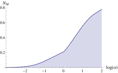
Before closing this section, we consider the Ohmic spectral density with an exponential cutoff , where is a dimensionless coupling strength and is the cutoff frequency. In this case, the full dynamics is still described by Eqs.(29) or (31), whereas the function is complex and is non-zero in general. For complex , the non-Markovianity has the following form,
| (45) | |||||
where , , and .
The exact value of for the Ohmic spectrum can be calculated using the analytic expressions in Ref.Zhang , that is,
| (46) | |||||
where . When the condition holds, corresponding to a dissipationless process () due to the zero spectral density for negative frequencies, otherwise, . Here is the solution of . The global phase in Eq.(46) is added compared with the expression in Ref.Zhang since we are working in the interaction picture for consistency with the Lorentzian case. In fact, the non-Markovianity does not depend on the picture we choose. The non-Markovianity for different (from to ) is calculated with , as shown in Fig.4. Although the system dynamics for the Ohmic spectrum is different from that for the lorentzian one, especially in the strong-coupling regime, the behavior of as a function of the coupling strength is similar. The non-Markovianity (memory effect) is non-zero for all even for parameters leading to in Eq.(31). When the coupling is weak, and (or ) are in a linear relationship in both cases, which indicates that the quantum process asymptotically becomes Markovian with the decreasing of the coupling strength.
VI Conclusions and Discussions
We present a criterion and propose a measure for non-Markovianity of quantum processes. The measure directly quantifies the degree of memory effects, i.e., how much the future state of a system depends on its past. To construct the measure, we introduce a universal dynamical map (UDM) which corresponds to an evolution starting from . In contrast to , is well defined and always CP as well as easy to calculate in a quantum process. The Markovian divisibility can be expressed in terms of in Eq.(19) and the violation of it is simply manifested by the inequality Eq.(20), which has a clear physical interpretation as the memory effects. We define non-Markovianity as the maximal violation of Eq.(19) for all times. Unlike the previous proposed measures which focus on evolutions starting from a fixed time, our measure applies to a quantum process where evolutions can starting at an arbitrary time.
One important result of our work is that a quantum process may have a memory effect even if it is called Markovian by other measures. Thus, the previously proposed criteria is not equivalent to the memory effect. Besides, we demonstrate that in a non-Markovian process, the dynamics may be still described by a time-dependent master equation in Lindblad-like form with non-negative decay rates. However, the non-Markovian master equation contains the initial time , which is essentially different from a time-dependent Markovian equation Chruscinski . When only describing evolutions starting from (), a non-Markovian master equation may have the same form of a time-dependent Markovian master equation, e.g., Eq.(30) with . By observing evolutions starting from different times as in Fig.2, memory effects can be revealed. Thus the negative decay rates in a master equation are not necessary to describe memory effects (non-Markovianity). And non-exponential but monotonic relaxation may occur in both non-Markovian processes and time-dependent Markovian processes.
Our measure is in units of trace distance that satisfies for any quantum process without normalization. It is easy to calculate regardless of the description of the quantum process. The optimization for quantum states or the knowledge of the environmental state is not required. When the full information of the dynamical map is unavailable, the condition [] can be used as an witness of non-Markovianity, which is easy to be examined both theoretically and experimentally.
Now we consider the renormalized spectral density with zero negative frequency components in the example where is the step function. By numerical simulation, we find that the dynamics and the non-Markovianity for are different from those for . The influence caused by a negative component strongly depends on . When are small, and leads to almost the same dynamics and non-Markovianity for both strong coupling (large ) and weak coupling. When are large, the negative frequency of the Lorentzian spectrum alters the dynamics and the non-Markovianity significantly for all coupling strengths (even for weak couplings). The reason is that is a symmetric function with the axis of symmetry and the peak width. Thus, determines the weight of the component of the negative frequency which in turn alters the correlation function and the dynamics evidently, whereas the non-Markovinity for is still non-zero for all and tends to as .
VII ACKNOWLEDGMENTS
We thank J. Cheng, H. Z. Shen and J. Nie for helpful discussions. This work is supported by the National Natural Science Foundation of China under Grant No. 11175032 and No. 61475033.
References
- (1) H.-P. Breuer and F. Petruccione, The Theory of Open Quantum Systems (Oxford University Press, London, 2007).
- (2) Á. Rivas and S. F. Huelga, Open Quantum Systems, An Introduction (Springer, Heidelberg, 2012).
- (3) D. Chruściński and A. Kossakowski, Phys. Rev. lett. 104, 070406 (2010).
- (4) J. Jing and T. Yu, Phys. Rev. Lett. 105, 240403 (2010).
- (5) F. F. Fanchini, T. Werlang, C. A. Brasil, L. G. E. Arruda, and A. O. Caldeira, Phys. Rev. A 81, 052107 (2010).
- (6) J.-S.Xu, C.-F. Li, M. Gong, X.-B. Zou, C.-H. Shi, G. Chen, and G.-C. Guo, Phys. Rev. Lett. 104, 100502 (2010)
- (7) K. H. Madsen, S. Ates, T. Lund-Hansen, A. Löffler, S. Reitzenstein, A. Forchel, and P. Lodahl, Phys. Rev. Lett. 106, 233601 (2011).
- (8) B.-H. Liu, L. Li, Y.-F. Huang, C.-F. Li, G.-C. Guo, E.-M. Laine, H.-P. Breuer, and J. Piilo, Nat. Phys. 7, 931 (2011).
- (9) W.-M. Zhang, P.-Y. Lo, H.-N. Xiong, M.W.-Y. Tu, and F. Nori, Phys. Rev. Lett. 109, 170402 (2012).
- (10) A. W. Chin, S. F. Huelga, and M. B. Plenio, Phys. Rev. Lett. 109, 233601 (2012).
- (11) S. F. Huelga, Á. Rivas, and M. B. Plenio, Phys. Rev. Lett. 108, 160402 (2012).
- (12) S. Deffner and E. Lutz, Phys. Rev. Lett. 111, 010402 (2013).
- (13) D. M. Kennes, O. Kashuba, M. Pletyukhov, H. Schoeller, and V. Meden, Phys. Rev. Lett. 110, 100405 (2013).
- (14) H. Tahara, Y. Ogawa, F. Minami, K. Akahane, and M. Sasaki Phys. Rev. Lett. 112, 147404 (2014).
- (15) J. Cerrillo and J. Cao, Phys. Rev. Lett. 112, 110401 (2014).
- (16) A. Shabani, J. Roden, and K. B. Whaley Phys. Rev. Lett. 112, 113601 (2014).
- (17) M. M. Wolf, J. Eisert, T. S. Cubitt, and J. I. Cirac, Phys. Rev. Lett. 101, 150402 (2008).
- (18) H.-P. Breuer, E.-M. Laine, and J. Piilo, Phys. Rev. Lett. 103, 210401 (2009).
- (19) E.-M. Laine, J. Piilo, and H.-P. Breuer, Phys. Rev. A 81, 062115 (2010).
- (20) R. Vasile, S. Maniscalco, M. G. A. Paris, H.-P. Breuer, and J. Piilo, Phys. Rev. A 84, 052118 (2011).
- (21) J. Liu, X.-M. Lu, and X. Wang, Phys. Rev. A 87, 042103 (2013).
- (22) Á. Rivas, S. F. Huelga, and M. B. Plenio, Phys. Rev. Lett. 105, 050403 (2010).
- (23) X.-M. Lu, X. Wang, and C. P. Sun, Phys. Rev. A 82, 042103 (2010).
- (24) S. Luo, S. Fu, and H. Song, Phys. Rev. A 86, 044101 (2012).
- (25) S. Lorenzo, F. Plastina, and M. Paternostro, Phys. Rev. A 88, 020102 (2013)
- (26) B. Bylicka, D. Chruściński, and S. Maniscalco, arXiv:1301.2585.
- (27) S. C. Hou, X. X. Yi, S.X.Yu, and C.H.Oh, Phys. Rev. A 83, 062115 (2011); S. C. Hou, X. X. Yi, S. X. Yu, and C. H. Oh, Phys. Rev. A 86, 012101 (2012).
- (28) A. K. Rajagopal, A. R. Usha Devi, and R. W. Rendell, Phys. Rev. A 82, 042107 (2010).
- (29) S. Alipour, A. Mani, and A. T. Rezakhani, Phys. Rev. A 85, 052108 (2012).
- (30) M. J. W. Hall, J. D. Cresser, L. Li, and E. Andersson, Phys. Rev. A 89, 042120 (2014).
- (31) D. Chruściński and S. Maniscalco, Phys. Rev. lett. 112, 120404 (2014).
- (32) G. Lindblad, Commun. Math. Phys. 48, 119 (1976).
- (33) Á. Rivas and S. F. Huelga, and M. B. Plenio, Rep. Prog. Phys. 77, 094001 (2014).
- (34) A. Gilchrist, N. K. Langford, and M. A. Nielsen, Phys. Rev. A 71, 062310 (2005)
- (35) M. Raginsky, Phys. Lett. A 290 11 (2011).
- (36) J. Watrous, Quantum Inf. Comput. 8, 819 (2008)
- (37) N. Johnston and D. W. Kribs, J. Phys. A: Math. Theor. 44 495303 (2011).
- (38) M. A. Nielsen and I. L. Chuang, Quantum Computation and Quantum Information (Cambridge University Press, Cambridge, 2000).
- (39) H.-P. Breuer, J. Phys. B 45, 154001 (2012).
- (40) T. J. G. Apollaro, C. Di Franco, F. Plastina, and M. Paternostro, Phys. Rev. A 83, 032103 (2011).
- (41) M.-D. Choi, Lin. Alg. and Appl. 10, 285 (1975).
- (42) A. Jamiołkowski, Rep. Math. Phys. 3, 275 (1972).