General-Purpose Join Algorithms
for Listing Triangles in Large Graphs

Abstract

We investigate applying general-purpose join algorithms to the triangle listing problem in an out-of-core context. In particular, we focus on Leapfrog Triejoin (LFTJ) by Veldhuizen[36], a recently proposed, worst-case optimal algorithm. We present “boxing”: a novel, yet conceptually simple, approach for feeding input data to LFTJ. Our extensive analysis shows that this approach is I/O efficient, being worst-case optimal (in a certain sense). Furthermore, if input data is only a constant factor larger than the available memory, then a boxed LFTJ essentially maintains the CPU data-complexity of the vanilla LFTJ. Next, focusing on LFTJ applied to the triangle query, we show that for many graphs boxed LFTJ matches the I/O complexity of the recently by Hu, Tao and Yufei proposed specialized algorithm MGT [10] for listing tiangles in an out-of-core setting. We also strengthen the analysis of LFTJ’s computational complexity for the triangle query by considering families of input graphs that are characterized not only by the number of edges but also by a measure of their density. E.g., we show that LFTJ achieves a CPU complexity of $O(|E|\log|E|)$ for planar graphs, while on general graphs, no algorithm can be faster than $O(|E|^{1.5})$. Finally, we perform an experimental evaluation for the triangle listing problem confirming our theoretical results and showing the overall effectiveness of our approach. On all our real-world and synthetic data sets (some of which containing more than 1.2 billion edges) LFTJ in single-threaded mode is within a factor of $3$ of the specialized MGT; a penalty that—as we demonstrate—can be alleviated by parallelization.

1 Introduction

Hu, Tao, and Yufei [10] recently proposed a novel algorithm (MGT) for listing triangles in large graphs that is both I/O and CPU efficient; and also outperforms existing competitors by an order of magnitude. At the same time, there has been exciting theoretical research that shows it is possible to design so-called worst-case optimal join algorithms [3, 36, 20, 21]. This begs the question: How would general-purpose join algorithms compare to the best specialized triangle-listing algorithms in a setting where not all data fits into main memory?

This question is motivated by the desire of building general-purpose systems that can empower their (domain) users to pose and run queries in a declarative and general language, such as SQL or Datalog—a goal that likely is little controversial. We focus on the out-of-core setting not only because of the obvious reasons of input or intermediary data not fitting in main memory, but also because we like to utilize graphics processing cards (GPUs) as high-throughput co-processors during query evaluation. GPU memory is currently limited to up to around 12GB [40], highlighting the urgency for robust out-of-core techniques.

The triangle listing is the basic building block for many other graph algorithms and key ingredient for graph metrics such as triangular clustering, finding cohesive subgraphs etc [10, 30, 31, 25]. In addition, it has gotten extensive attention in the research literature among several fields: graph theory, databases and network analysis to name a few. Here, both in-memory as well as in an out-of-core algorithms have been studied. Having a general-purpose technique being able to compete with the best-in-class hand-crafted algorithms that are specific for triangle listing, would indeed, be very good news for the database community advocating high-level, declarative query languages.

We selected Leapfrog-Triejoin (LFTJ) by Veldhuizen as the general-purpose join algorithm for our study. This is for various reasons: (1) its elegance allows efficient implementations with various optimizations, (2) by nature, LFTJ only uses $O(1)$ intermediary data, making it a very good candidate in the out-of-core context, and (3) because of its strong theoretical worst-case guarantees [36]. LFTJ’s worst-case guarantee in its generality is technical [36]. Roughly, it guarantees that for a given query and input $I$, LFTJ will never perform asymptotically more steps (up to a log-factor) than what are strictly necessary for any correct algorithm on inputs $I^{\prime}$ that are similar to $I$. Here, similar means that, eg., the sizes of the input relations cannot change nor can certain other statistics of the data.

Model & Assumptions. We restrict our attention to full-conjunctive queries, and use a Datalog syntax and terminology to describe queries (or joins). Our formal setting is the standard one for considering I/O efficient algorithms: Input, intermediary and output data can exceed the amount of available main memory $M$ (measured in words to store one atomic value), in which case it can be read (written) from (to) secondary storage with the granularity of a block that has size $B$. Reading or writing a block incurs 1 unit of I/O cost. For I/O and CPU cost, we consider data complexities, that is we assume the query to be fixed and small. In particular, we like $M/B$ to be larger than, say 10 times, the number of atoms multiplied by their maximum arity. Furthermore, to simplify complexity results, we assume that $|I|/B$ is larger than $\log|I|$. This restriction is mostly theoretic: Using a block size of 64KiB with a 64-bit word-width, inputs only need to be larger than 15MiB to satisfy the requirement. With these assumptions in mind, we make the following contributions:

Contributions

Boxing LFTJ. We present and analyze a novel strategy we call boxing for out-of-core execution of a multi-predicate, worst-case optimal join algorithm (Leapfrog-Triejoin). This method exhibits the following properties:

(1) For queries with $n$ variables, executing on input data $I$ and producing output data of size $K$, boxed LFTJ requires at most $O(|I|^{n}/(M^{n-1}B)+K/B)$ block I/Os. We show that this bound is worst-case optimal, in the sense that for any $n$, we can construct a query such that no algorithm can have an asymptotically better bound with respect to $I$ and $K$.

(2) We further show that if the input data exhibits limited skew (in the sense we will make precise) then boxed LFTJ requires only $O(|I|^{r}/(M^{r-1}B)+K/B)$ I/Os. Here, $r$ denotes the rank of the query—a property we will define. The rank of a query never exceeds the number of variables used in the Datalog body, and is often lower.

(3) We also analyze the computational complexity of boxed LFTJ. Here, we show that if the input size $|I|$ is only a constant factor larger than the available memory $M$, then the asymptotic CPU work performed by the boxed LFTJ (essentially) matches the asymptotic complexity of the in-memory LFTJ maintaining its theoretical guarantees.

Boxed $\textnormal{{LFTJ-}}\mathbf{\Delta}$. We apply boxing to the triangle-listing problem. Here, the input graph exhibits limited-skew if the degree of its nodes is limited by $M/9$. With 100GiB of main memory this allows graphs containing nodes with up to 1.3 million neighbors.

On such graphs, our approach requires $O(|I|^{2}/(MB)+K/B)$ block I/Os, matching the asymptotic I/O bound of the recently presented specialized algorithm MGT [10] for triangle listing.

In-memory $\textnormal{{LFTJ-}}\mathbf{\Delta}$. We also tighten the analysis for the CPU complexity of the conventional in-memory LFTJ applied to the triangle listing query with non-trivial arguments. It is easy to see that $\textnormal{LFTJ-}\Delta$’s achieved asymptotic complexity of $O(|E|^{1.5}\log|E|)$ is worst-case optimal modulo the log-factor. We improve on this result in two ways:

(1) We show that for graphs $G=(V,E)$ with an arboricity $\alpha(|E|)$, $\textnormal{LFTJ-}\Delta$ requires $O(|E|\alpha(|E|)\log|E|)$ work. A graph’s arboricity is a measure of its density (as we will explain later) which never exceeds $O(\sqrt{|E|})$. Moreover, $\alpha$ is substantially smaller for many graphs [7, 15]; for example, for both planar graphs and graphs with fixed maximum degree, $\alpha\in O(1)$. As a corollary, we thus obtain that $\textnormal{LFTJ-}\Delta$ runs in $O(|E|\log|E|)$ on planar graphs.

(2) We further improve on the worst-case optimality analysis: We show that even if we are only interested in families of graphs for which their arboricity is limited by any function $\hat{\alpha}\in o(\sqrt{|E|})$, e.g. by $30\log|E|$, and we would like to design a specialized algorithm that (only) works (well) on these graphs, then this algorithm cannot have an asymptotic complexity that is in $o(\hat{\alpha}(|E|)|E|)$. This result shows that $\textnormal{LFTJ-}\Delta$ is worst-case optimal for any of these families (modulo the log-factor).

Evalation. We further present an experimental evaluation, where we focus on the triangle query. We confirm that the boxing technique works well, especially when the input data is only a constant factor larger than the available memory: on real-world and synthetic graphs with each more than 1.2 billion nodes, boxing only introduces little CPU overhead; and has good performance even when only limited main memory is available. We also compare the raw performance against two competitors: a specialized [32] C++-based implementation in the graph-processing system Graphlab [16] and the specialized triangle listing algorithm MGT [10]. LFTJ is about 65% the Graphlab implementation, yet scales to larger data sizes. When running single-threaded, LFTJ is on average 3x slower than MGT. Our parallelized version of LFTJ, however, is slightly faster than the single-threaded MGT (about 30% main memory is restricted to as much as 10%

The rest of the paper is structured as follows: Section 2 reviews the relevant background information. We present and analyze the boxing strategy for LFTJ in Section 3. Section 4 analyzes the in-memory and the boxed variant of LFTJ applied to the triangle query. Section 5 highlights some important aspects of our implementation, before we experimentally evaluate our approaches in Section 6. We review related work in Section 7 and conclude in Section 8.

2 Background

2.1 Review: Leapfrog-Triejoin (LFTJ) [36]

LFTJ [36] is a multi-predicate join algorithm. Unlike traditional binary join algorithms such as Hash-Join or Sort-Merge-Join which take two relations as input, LFTJ takes as input $n$ relations together with the join conditions.

Example 1 (LFTJ).

Consider the query:

$$Q(x,y,z)\leftarrow R(x,y),S(x,z),T(y,z).$$

With binary joins, we first join, e.g., $R(x,y)$ with $S(x,z)$ to obtain $RS(x,y,z)$ and then join $RS(x,y,z)$ with $T(y,z)$ to obtain $Q(x,y,z)$. LFTJ, on the other hand directly computes $Q(x,y,z)$ given all predicates in the body of the rule as an input without storing any sizeable intermediary results.

Some notation is necessary: for a binary relation $R(x,y)$, let $R(x,\_)$ denote the set of values in the first column, i.e., $R$ projected to its first attribute; further let $R_{a}(y)$ denote the projection to the second attribute after only selecting tuples that have the constant $a$ as the first attribute.

LFTJ operates by first fixing an order of the variables occuring in the rule body. In our example, we might pick $x,y,z$ as the order. Then, LFTJ finds all possible values $a$ for the variable $x$. This is done by performing an intersection of $R(x,\_)$ and $S(x,\_)$, i.e., the first column of $R$ with the first column of $S$ because the variable $x$ occurs in these atoms. Now, as soon as the first of such $a$ is found, LFTJ is looking for values $b$ of $y$, the next variable in the variable-order. Here, LFTJ computes the intersection of $R_{a}(y)$ and $T(y,\_)$. Again, as soon as the first of such $b$ is found, LFTJ is looking for values $c$ for $z$ by computing the intersection of $S_{a}(z)$ and $T_{b}(z)$. If any of these $c$ is found LFTJ reports the tuple $(a,b,c)$ in the output. Once the intersection of $S_{a}(z)$ and $T_{b}(z)$ has been computed, LFTJ back-tracks its search to the variable $y$ and looks for the next $b^{\prime}$. Back-tracking continues up to the first variable and LFTJ finishes when no new $a^{\prime}$ can be found anymore. A key to LFTJ’s performance is to efficiently compute the various intersections. This is achieved via the method of a Leapfrog join (LFJ) which, as we detail below, leverages that relations are pre-sorted.

Trie representation for relations.

(a) $R$

(b) Trie of $R$

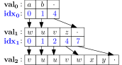
(c) TrieArray of $R$

Figure 1: Trie and TrieArray of a ternary relation $R$

It is convenient to think of relations to be represented as a Trie. A Trie is a tree that stores each tuple of a relation as a path from the root node to a child node. See Fig. 1(a) for an example of a ternary relation with its trie in Fig. 1(b). In general, a Trie for a relation with arity $a$ has a height of $a$. For a relation $R(x_{1},\dots,x_{a})$, the nodes at height $i$ store values from the $i$th column of $R$. We require that children of the same node $n$ are unique and ordered increasingly. For example in Fig. 1(b) at level 2, the children of b are the values u, v, and w, which are in increasing order.

TrieIterators. LFTJ accesses relational data not directly but via a TrieIterator interface. This not only allows various storage schemes but also facilitates uniform handling of “infinite” predicates such as Equal, SmallerThan or Plus. The TrieIterator interface provides methods to navigate the Trie of a relation. It can be thought of as a pointer to a node in the Trie. The detailed methods for Trie navigation are given in Apx. A.1. The methods are value() to access a data value; open() and close() to move up and down in the trie. The linear iterator methods next, seek, and atEnd are used to move within unary “sub-relations” $A$ such as $R(x,\_)$ or $R_{a}(y)$. Here, next moves one step right and seek() is used to forward-position the iterator to the element with value $v$; if $v$ is not in $A$, then the iterator is placed at the element with the smallest value $w>v$. In general, if the iterator passes the end of the represented relation such as $R_{a}(y)$, the atEnd will return true. A key to good LFTJ performance is that back-end data structures efficiently support these TrieIterator operations. In fact, the theoretical guarantees given by LFTJ require that value, key, atEnd have complexity $O(1)$. Furthermore, seek and next must not take longer than $O(\log N)$ individually and must have an armortized cost of at most $O(1+\log(N/m))$ if $m$ keys are visited. Here, $N$ stands for the size of the unary relation the iterator is for; eg, $R_{a}(y)$.

Leapfrog Join. A basic building block of Leapfrog Triejoin (LFTJ) is Leapfrog join (LFJ). It computes the intersection of multiple unary relations. For this, LFJ has a linear iterator for each of its input relations. An execution of LFJ is reminiscent of the merge-phase of a merge-sort; however instead of returning values that are in any of the inputs, we search and return values that are in all input relations. To do so efficiently, we use seek to iteratively advance the iterator positioned at the relation with the smallest value to the largest value amongst the iterators. If all iterators are placed on the same value, we have found a value of the intersection.

Using LFJ to join $n$ relations with $N_{\min}$ and $N_{\max}$ denoting the cardinalities of the smallest and largest relation, respectively, has the following complexity:

Proposition 2 (3.1 in [36]).

The running time of Leapfrog join is $O(N_{\min}\log(N_{\max}/N_{\min}))$.

The detailed algorithms for the Leapfrog join as well as LFTJ are given in Apx. A as reference; for an even more detailed introduction and reference see [36].

Leapfrog TrieJoin Restrictions. LFTJ requires that no variable occurs more than once in a single body atom. This can be achieved via simple rewrites: Given a join with, e.g., the atom $A=R(x,y,x)$ in the body, we introduce a new variable $x^{\prime}$ and replace $A$ by $R(x,y,x^{\prime}),\mathtt{Eq}(x,x^{\prime})$ where $\mathtt{Eq}$ is the infinite equal-relation which itself is represented by a specialized TrieIterator.

As mentioned above, LFTJ is parameterized by an order on the variables of the join. This order is usually chosen by an optimizer as the exact order might influence runtime characteristics and can have an effect on the theoretical bounds for the I/O complexity as we will detail below. Furthermore, the chosen order determines the sort-order of the input relations: In particular, arguments in atoms of the join body must form a subsequence of the chosen order. E.g., consider the order $x,y,z$: body atoms $R(x,z)$ or $S(y)$ are allowed while the atom $T(y,x)$ needs to be replaced by an alternative index $T_{2,1}(x,y)$ which is created as $T_{2,1}(x,y)\leftarrow T(y,x)$. These indexes are created in a pre-processing step.

2.2 TrieArrays

We use a simple array-encoding for Tries, which is inspired by the Compressed-Sparse-Row (CSR) format—a commonly used format to store graphs. As an example see Fig. 1(c) for the representation of the trie given in Fig. 1(b). The data values are stored in flat arrays called value-arrays. Index arrays are used to separate children at the same tree level but from different parent nodes. An $n$-ary relation has $n$ value arrays and $n-1$ index arrays. In particular, the children of a node $n$ stored in the value array $\mathbf{val_{i}}$ at position $j$ are stored in the array $\mathbf{val_{i+1}}$ starting at the index from $\mathbf{idx_{i}}[j]$ until the index $\mathbf{idx_{i}}[j+1]$ inclusively. E.g. in Fig. 1(c), the children $w,x,y$ of $w$ from $\mathbf{val_{1}}[3]$ are stored in $\mathbf{val_{2}}$ from $\mathbf{idx_{1}}[3]=4$ to $\mathbf{idx_{1}}[4]=7$.

To reduce notation, we will often simply identify a relation $R$ with its TrieArray representation and vice versa in the rest of the paper. For example, when we write a $n$-ary TrieArray we mean a TrieArray for an $n$-ary relation $R$.

All TrieIterator operations are trivial to implement for TrieArrays; except possibly seek, where some attention needs to be given to achieve the required armortized complexity. Here, instead of starting the binary in the middle of the remaining sub-array, we probe with an exponentially increasing lookup sequence of eg., $1,4,16,64,...$ to narrow lower and upper bounds for the binary search.

While the TrieArray representation is beneficial for execution, it is also fairly cheap to create:

Proposition 3.

The TrieArray representation of a relation $R$ requires no more than $O(|R|)$ space and can be built in $O(SORT(R))$ time and I/O complexity.

Sketch. The space requirement is obvious; furthermore the data structure can be built from a lexicographically sorted $R$ in two passes: pass 1 determines the sizes of the value and index arrays, pass 2 fills in data.

2.3 LFTJ for Computing Triangles

Given a simple, undirected graph $G$ and let ${G}^{\star}=(V,E)$ be its directed version, that is for each edge $\{a,b\}\in E(G)$, $E$ contains the pair $(\min\{a,b\},\max\{a,b\})$. The query

$$T(x,y,z)\leftarrow{E}(x,y),{E}(x,z),{E}(y,z),x<y<z.$$

computes all triangles in ${G}^{\star}$ of the form: . The output $T$ coincides with the triangles in $G$. Since $x<y<z$ is already implied by the atoms containing the edge relation, we can omit the inequality from the query obtaining:

$$T(x,y,z)\leftarrow{E}(x,y),{E}(x,z),{E}(y,z). \Delta$$ ()

3 Boxing LFTJ

We first motivate our strategy by showing that LFTJ can suffer from excessive I/O operations in an external-memory setting with a block-based least-recently-used memory replacement strategy. As example, we use the triangle query with specifically crafted input graphs.

LFTJ on the triangle query. It is useful to highlight the steps that LFTJ performs for the triangle query ($\Delta$). These are summarized in Algorithm 1. Note that Algorithm 1 is not the pseudo-code of the program we use to list triangles; it only summarizes the steps LFTJ performs when run on the triangle query. First, the leapfrog join at level $x$ for the atoms $E(x,y)$ and $E(x,z)$ computes the intersection between $E(x,\_)=V_{1}$ and $E(x,\_)=V_{1}$. Then, for each found value $a$ for $x$, we perform a leapfrog-join at level $y$ computing the intersection of $E_{a}(y)=D(a)$ with $V_{1}=E(y,\_)$, because the variable $y$ occurs in the atoms $E(x,y)$ and $E(y,z)$. In the last step, we find bindings for $z$ by intersecting $D(a)=E_{a}(z)$ with $D(b)=E_{b}(z)$ because $z$ occurs in the atoms $E(x,z)$ and $E(y,z)$.

Algorithm 1 Steps Performed by Leapfrog-Triejoin on the Triangles Query $T(x,y,z)\leftarrow E(x,y),E(x,z),E(y,z)$.

1:for $a\in V_{1}\cap V_{1}$ do $\triangleright$ $V_{1}:\!\!\leavevmode\resizebox{5.71527pt}{0.0pt}{=}\,\{x\,|\,(x,v)\in E\}$

2:     for $b\in V_{1}\cap D(a)$ do $\triangleright$ $D(v):\!\!\leavevmode\resizebox{5.71527pt}{0.0pt}{=}\,\{x\,|\,(v,x)\in E\}$

3:         for $c\in D(a)\cap D(b)$ do

4:              yield $(a,b,c)$ $\triangleright$ triangle found               

Example inputs that causing excessive I/O. For $N\geq M+B$, consider the graph $G_{N}=(V,E)$ with edges $E$ as:

$$E=\{(x,y)\,|\,x=0,\dots,N\textnormal{ and }y=N-B(x\textnormal{ mod }T)\}$$

where $T=M/B+1$ being slightly larger than the number blocks fitting into main memory at once. See Fig. 12(a) in the appendix for an example with $N=24$, $M=20$, $B=4$, and $T=6$. The key idea is that we place values in the second column of $E$ by $B$ apart which will cause LFTJ to perform an I/O for every tuple in $E$ for step 3 in Algorithm 1; furthermore, we make sure values in the second column repeat in groups large enough that loading all blocks in a group will preempt the first block from memory effectively prohibiting the algorithm to reuse the earlier loaded blocks.

Proposition 4.

$\textnormal{LFTJ-}\Delta$ incurs at least $2|E(G_{N})|$ I/Os for the above defined graph $G_{N}$ with a TrieArray data representation and a LRU memory replacement strategy.

Proof.

See Apx. B.1.

3.1 High-Level Idea

(a) Graph $G$

$\begin{array}[]{|r||c|c|c|c|c|c|c|c|c|c|c}\hline\cr\mathbf{x}&1&1&1&2&2&3&4&4&5&6\\ \hline\cr\mathbf{y}&2&3&6&4&5&6&5&7&7&7\\ \hline\cr\end{array}$

(b) $E=E({G}^{\star})$

(c) Dir. graph ${G}^{\star}$

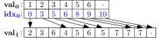
(d) TrieArray $T$ for $E=E({G}^{\star})$

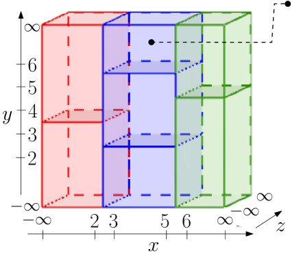
(e) Boxed Search Space

Box $[3\cdot\!\cdot\!\cdot 5,6\cdot\!\cdot\!\cdot\infty,-\infty\cdot\!\cdot\!\cdot\infty]$        

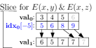
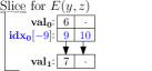
(f) Example Box & TrieSlices

Figure 2: Example for out-of-core technique for $\textnormal{LFTJ-}\Delta$, i.e. $T(x,y,z)\!\!\leftarrow\!\!E(x,y),E(x,z),E(y,z)$ on $E({G}^{\star})$

We now describe our out-of-core adaptation for LFTJ. LFTJ with a variable order $x_{1},\dots,x_{n}$ computes the join by essentially searching over an $n$ dimensional space in which each dimension $i$ spans over the domain of the variable $x_{i}$. Loosely speaking, the space is searched in lexicographical order. As the example above demonstrates, this can lead to excessive I/O costs. Further I/O accesses are caused by the potentially non-local accesses for the binary searches of leapfrog-join.

In our approach, we partition the $n$-dimensional search space into “hyper-cubes” or boxes such that the required data for an individual box fits into memory. LFTJ is then run over each box individually—finding all input data ready in memory. We strive for the following properties: (i) Determining box-boundaries is efficient: both in CPU and I/O work. (ii) Loading data that is restricted to a box is efficient, again, both in terms of CPU and I/O work. (iii) The total amount of data loaded is minimal.

Fig. 2 illustrates this strategy for $\textnormal{LFTJ-}\Delta$. The join uses three variables $x$, $y$, $z$ – resulting into a 3-dimensional search-space. If the input graph $G$ represented via a TrieArray does not fit into the available memory, then we partition the search space into boxes, for example as in Fig. 2(e). The partitioning is chosen such that the input data restricted to an individual box fits into memory. $\textnormal{LFTJ-}\Delta$ is then run for each box individually one after another while join results are written append-only in a streaming fashion.

We now explain the different aspects in detail.

3.2 TrieArray Slices

We assume that input data is given on external storage in a TrieArray representation, with the attribute order consistent with the chosen key order for LFTJ. This can easily be achieved via a pre-processing step that costs $O(SORT(|I|)$ block I/O and CPU steps. When loading data for a single box into main memory, we directly operate on the TrieArray representation to subset the data. The remainder of this subsection shows that this step can be done very efficiently.

In general, applying any selection $\sigma$ to a TrieArray for a predicate $R$ to obtain a TrieArray for $\sigma(R)$ can be done in $O(|R|)$ cpu work and $O(|R|/B)$ I/Os if $\sigma(t)$ can be computed in $O(1)$ time and space for tuples $t\in R$. This is because TrieArrays can be used to efficiently enumerate the represented tuples in lexicographically order, and they can also efficiently be built from lexicographically sorted tuples.

We are interested in certain range-based selections. It turns out that these can be built even faster—with costs proportional to the selected size $|\sigma(R)|$ rather then the total data set size $|R|$ (modulo log-factor), or even less depending on the cost-model.

Example 5 (TrieArray Slice).

Consider the binary relation $E$ from Fig. 2(c) and its TrieArray $T$ in Fig. 2(d). We are interested in the subset $S$ of $T$ that restricts the first attribute to the interval $[3,5]$, i.e., $S=\{(x,y)\in T\,|\,x\in[3,5]\}$. We call this a slice of $S$ at level $0$ from $3$ to $5$. A TrieArray for this slice is shown at the top of Fig. 2(f). To build this slice, we can simply copy the values in $\mathbf{val_{0}}$ for the interval $[3,5]$; then look up where the corresponding $y$ values are in $\mathbf{idx_{0}}$, and copy these as well. The index value cannot simply be subset because the positions need to be shifted by the amount we cut off from $\mathbf{val_{1}}$ in the front: the first index in $\mathbf{idx_{0}}$ of the slice should read $0$ instead of $5$. However, instead of changing the values, we add a wrapper to the index arrays that can subtract the offset (here 5) during accesses dynamically. Then, all data used in the arrays of the slice are simply sub-arrays of the original data.

In general, for an $n$-ary relation $R$, we are interested in creating slices at a level $k$, $0\leq k<n$. At level $k$ the values are restricted to an interval given by a low-bound $l$ and a high-bound $h$; at levels $0,\dots,k-1$, the slice contains only a single element each. Formally:

Definition 6 (Slices).

Let $R$ be an $n$-ary relation, $0\leq k<n$ an integer, $s$ be a $k$-ary tuple, and $l$ and $s$ be two domain values. The Slice $S$ of $R$ at level $k$ for $s$ from $l$ to $h$ (in symbols $S={R}^{s}_{l\rightarrow h}$) is the defined as:

$$S=\{(x_{0},...,x_{n-1})\in R\,|\,(x_{0},...,x_{k-1})=s\textnormal{ and }l\leq x_{k}\leq h\}$$

We often do not mention the level explicitly as it is evident from the start tuple $s$; also, if $k=0$, we simply say “Slice for $R$ from $l$ to $h$”.

We create and store Slices in the TrieArraySlice data structure, which is a conventional TrieArray—except that the index arrays can be parameterized with an offset to perform dynamic index-adaptation as explained in the example above. As with TrieArrays, we identify the Slice (set of tuples) with the TrieArraySlice data structure and vice versa in the rest of the paper.

Given a relation $R$ on secondary storage, we can create slices of $R$ efficiently:

Proposition 7 (Slice provisioning).

Let $R$ be an $n$-ary relation stored on secondary storage as a TrieArray; $k,s,l,$ and $h$ be as in Def. 6. Then, the slice $S={R}^{s}_{l\rightarrow h}$ can be loaded into memory with $O(\log|R|+|S|/B)$ block I/Os and $O(\log|R|+|S|/B)$ CPU work, if it fits.

Sketch The provisioning process is as follows: using $k$ binary searches on the value arrays $\mathbf{val_{0}},\dots,\mathbf{val_{k-1}}$, we locate the prefix $s$ in $R$; the slice is empty if the prefix does not exist. Then, using two more binary searches we locate the smallest element $l^{\prime}\geq l$ and the largest $h^{\prime}\leq h$ in $\mathbf{val_{k}}$ of $R$. Their positions are the boundaries in $\mathbf{val_{k}}$ and $\mathbf{idx_{k}}$ for the interval we copy into the slice. For the remaining $n-k$ value arrays and $n-k-1$ index arrays, we iteratively follow the pointers within the $\mathbf{idx}$ arrays and copy the appropriate ranges. As a last step we adjust the index-array’s offset parameter: for each $j=k,\dots,n-2$, we set the offset parameter of $\mathbf{idx_{j}}$ to $-\mathbf{idx_{j}}[0]$.

We require $O(\log|R|)$ I/Os for the binary searches and $O(|S|/B)$ I/Os for copying the continuous values from the arrays with indexes $\geq k$. Similarly, the binary searches require $O(\log|R|)$ CPU work; the remaining CPU work accounts for requesting the copy operations.

Note that besides the logarithmic component, provisioning a slice amounts to simply copying large, continuous arrays from secondary storage into main memory. On modern hardware, these can be done using DMA methods without causing any significant CPU work. Moreover, modern kernels might simply memory map the to-be-copied pages and perform actual copies only when pages are modified.

Probing. As the last building block, we are interested in provisioning slices that will fill up a certain budgeted amount of memory. In particular, we specify the prefix-tuple $s$ and lower bound $l$ as before. But instead of providing an upper bound $h$, we give a memory budget $m$ in blocks as shown in Fig. 3. We are then interested in a maximal upper bound $h\geq l$ such that the slice at $s$ from $l$ to $h$ requires no more than $m$ blocks of memory. Note that for skewed data, it is possible that the slice ${T}^{s}_{l\rightarrow h}$ requires more than $m$ blocks of memory, even when $h=l$. Should this case occur, we report via the sentinel value SPILL instead of returning an upper bound $h$. Not surprisingly, probing is also efficient:

Proposition 8.

For a TrieArray $T$ on secondary storage, probing the upper bound for a Slice to fill up a memory budget as described in Fig. 3 requires $O(\log|T|)$ I/Os and CPU work.

Sketch Similar to slice provisioning, except that we do a binary search for the upper bound and check for each guess how many blocks the TrieSlice would occupy. This can be done by following the $\mathbf{idx_{i}}$ pointers. Determining the size of the TrieSlice for each guess requires at most $O(n)$ I/Os where $n$ is the arity of $T$. Since we binary search in $\mathbf{val_{k}}$, an array that is at most size $|R|$, we obtain the required complexity of $O(\log|R|)$.

 

function Probe($T$, $s$, $l$, $m$) returns $h$

in: $n$-ary TrieArray $T$ $\triangleright$ on secondary storage

in: $k\mathsf{\textnormal{-}\!Tuple}$ $s$ $\triangleright$ start tuple for attributes $0,\!..,k-1$

in: value $l$ $\triangleright$ Lower bound for attribute  $k$

in: $\mathsf{int}$ $m$ $\triangleright$ memory budget in blocks

out: Maximal $h\geq l$ such that the slice ${T}^{s}_{l\rightarrow h}$ occupies

out: $\leq m$ blocks of memory, or SPILL if no such $h$ exist.

 

Figure 3: Interface for Single Slice Probing

3.3 Boxing Procedure

To help exposition, we first describe aspects of the boxing approach via examples, before we cover the general case.

Joins with one variable. Consider a join over multiple unary relations such as

$$Q(x)\leftarrow R(x),S(x),T(x).$$

Imagine each of the body relations is larger than the available internal memory $M$. We can divide the internal memory into four parts, one for the output data and one for each of the input relations. Since the output is written append-only, a relatively small portion of memory, which is written to disk once it fills up, is sufficient. We thus divide up the bulk of the memory for the three input relations. We can use the simple strategy to evenly divide the space. A boxed LFTJ execution would then simply alternate probing, provisioning, and calling LFTJ as described in Fig. 4.

 

1:$l$ $\leftarrow$ $-\infty$ $\triangleright$ Value at the start of the search space

2:repeat

3:     probe $R,S,T$ from $l$ for upper bounds $h_{R}$, $h_{S}$, $h_{T}$

4:     $h\leftarrow\min(h_{R},h_{S},h_{T})$

5:     provision $R,S,T$ from $l$ to $h$

6:     run LFTJ on the provisioned slices

7:     $l\leftarrow\mathsf{succ}(h)$ $\triangleright$ lower bound is successor of old upper

8:until $\infty=h$ $\triangleright$ until we have searched all space

 

Figure 4: Example: Boxing for $R(x),S(x),T(x)$

Not surprisingly, this approach would work well for the limited class of joins: for reading the input, it requires a number of I/Os bound by $O(|I|/B+|I|/M\log|I|)$ with $|I|$ being the combined size of the input relations. The key observations for showing the bound is that in each iteration (except possibly the last), at least one relation will load $O(M)$ (in our example around $M/3$) tuples using $O(M/B)$ block reads. Now, since there are only $|I|$ tuples in the input, there are at most $O(|I|/M)$ iterations. Since each probing can be done in $O(\log|I|)$ we obtain the desired bound.

 

1:variables: $m\mathsf{\textnormal{-}\!Tuple}$ low, high $\triangleright$ Box boundaries

2:procedure Main

3:     BoxUp(1)

4:procedure BoxUp($\mathsf{int}$ $i$) $\triangleright$ $i$ corresponds to $x_{\textnormal{$i$}}$

5:     $\textnormal{low}[\textnormal{$i$}]$ $\leftarrow$ $-\infty$

6:     repeat

7:         probe inputs $R_{i}$ from $\textnormal{low}[\textnormal{$i$}]$ for upper bound $h_{i}$

8:         $\textnormal{high}[\textnormal{$i$}]\leftarrow h_{i}$

9:         provision $R_{i}$ from $\textnormal{low}[\textnormal{$i$}]$ to $\textnormal{high}[\textnormal{$i$}]$

10:         if $\textnormal{$i$}<m$ then : BoxUp(i+1)

11:         else: run LFTJ on slices $\triangleright$ Box: $[\textnormal{low}\!\cdot\!\cdot\!\cdot\!\textnormal{high}]$          

12:         $\textnormal{low}[\textnormal{$i$}]\leftarrow\mathsf{succ}(\textnormal{high}[\textnormal{$i$}])$

13:     until $\infty=\textnormal{high}[\textnormal{$i$}]$

 

Figure 5: Example: Boxing for $R_{1}(x_{1}),\!...,R_{m}(x_{m})$

Unary cross-products. Consider the cross-product of $m$ unary relations, with each relation larger than $M$:

$$Q(x_{1},\!...,x_{m})\leftarrow R_{1}(x_{1}),\dots,R_{m}(x_{m}).$$

We again split the bulk of the available memory across the $m$ input relations. The boxing procedure is recursive where each dimension $i$ of the recursion corresponds to a variable $x_{i}$ (See Fig. 5). The procedure starts with $\textnormal{$i$}=1$. In general, at a dimension $i$, we loop over the predicate $R_{i}$ via the probe-provisioning loop. Then, for each slice at dimension $i$, we do the same recursively for the next higher dimension. At the bottom of the recursion—when we reached the $i=m$, we call LFTJ on the created slices. Then, the slices provide data for the box $[\textnormal{low}\!\cdot\!\cdot\!\cdot\!\textnormal{high}]$, i.e., in which the variable $x_{i}$ can range from $\textnormal{low}[\textnormal{$i$}]$ to $\textnormal{high}[\textnormal{$i$}]$. Note that (like above) we can run the original query over the slice data since the slices are guaranteed to not have data outside their range and thus the boxes partition the search-space without overlap.

General joins. The general approach combines the two previous algorithms while also considering corner cases. Let $Q$ be a general full-conjunctive join of $m$ atoms, and variable order $\pi=x_{1},\dots,x_{n}$ with no atom containing the same variable twice, and all atoms in $Q$ mentioning variables consistent with $\pi$. We first group the atoms based on their first variable $x_{j}$: we place all atoms that have as first variable $x_{j}$ into the array $\textnormal{atoms}[1..n]$ at position $j$. To follow the exposition, consider the join

$$Q(x_{1},x_{2},x_{3})\leftarrow R(x_{1},x_{2}),S(x_{1},x_{3}),T(x_{2},x_{3}),U(x_{1})$$

where we put $R,S$, and $U$ into $\textnormal{atoms}[1]$ and $T$ into $\textnormal{atoms}[2]$. Like for cross-products, we recursively provision for the dimension $i$ ranging from $1$ to $n$. For each $i$, we use the method for joining unary relations for the atoms in $\textnormal{{atoms}}[i]$. In particular, for each $A_{j}\in\textnormal{atoms}[i]$ we probe and create slices for $A_{j}$ at level 0 regardless of $i$ or the arity of $A_{j}$. Thus, at dimension $i$, we iteratively provision atoms with $x_{i}$ as their first attribute restricting the range of $x_{i}$ but not any of the other variables $x_{k}$, $k>i$. This ensures that we can freely choose any partitions we might perform on these variables $x_{k}$ for $k>i$. Like with cross-products, we call LFTJ at the lowest level when $i=n$.

The above works well unless any of the probes reports a SPILL, which can occur if a relation exhibits significant skew. For example, imagine there is a value $a$ for which $|S_{a}(x_{3})|$ exceeds the allocated storage. Then, at dimension $i=1$, probing $S$ at level $0$ with a lower bound $a$ will return SPILL. We handle these situations by setting the upper bound at level $i=1$ to $a$, and essentially marking $S_{a}$ as a relation that needs to be provisioned at the dimension of its second attribute (eg, 3) alongside the atoms in $\textnormal{{atoms}}[3]$. Note that a relation of arity $\alpha$ can spill $\alpha-1$ times in worst case.

The general algorithm is given in Algorithm 2. We evenly divide the available storage among the $n$ dimensions, and assign the atoms $A$ to $\textnormal{{atoms}}[\textnormal{$i$}]$ accordingly (lines 3-4). We also use a variable leftoverMem to let lower dimensions utilize memory that was not fully used by higher dimensions. In line 11, we union the spills from the previous level to the atoms we need to provision. The method probe in line 12, probes atoms in atms to find an upper bound such that all atoms can be provisioned. We here, evenly divide mem by the size of atms. The lower bound for probing are taken from low, which is also used to determine the starting tuples for possible spills. The method sets the upper bound at the current dimension and fills the spills predicate if necessary. The method provision provisions the predicate $A$ with bounds from low and high adapted to the variables occuring in $A$. It returns the slice and the size of used memory.

Algorithm 2 Boxing Leapfrog Triejoin

1:in: $\textnormal{mem}_{max}$$\triangleright$ available memory in blocks

2:in: $A_{1},\dots,A_{m}$ $\triangleright$ body atoms and TrieArrays

3:in: $x_{1},\dots,x_{n}$ $\triangleright$ key order, $n$ variables

4:variables:

5:in: $n\mathsf{\textnormal{-}\!Tuple}$ low, high $\triangleright$ Box boundaries

6:in: $\mathsf{Array\;of}$ $\mathsf{AtomSet}$ $\textnormal{atoms}[1..n]$ $\triangleright$ atoms per level

7:in: $\mathsf{Array\;of}$ $\mathsf{SliceSet}$ $\textnormal{S}[1..n]$ $\triangleright$ provisioned slices

8:in: $\mathsf{Array\;of}$ $\mathsf{AtomSet}$ $\textnormal{spill}[0..n]$ $\triangleright$ spilled-over atoms

9:in: $\mathsf{Array\;of}$ $\mathsf{int}$ $\textnormal{budget}[1..n]$ $\triangleright$ of memory in blocks

10:

11:procedure Main

12:     for $\textnormal{$i$}\in\{1,\dots,n\}$ do

13:         $\textnormal{budget}[\textnormal{$i$}]$ $\leftarrow$ $\textnormal{mem}_{max}/n$

14:         $\textnormal{atoms}[\textnormal{$i$}]$ $\leftarrow\{A_{\textnormal{$i$}}\,|\,x_{\textnormal{$i$}}\textnormal{ is first variable in }A_{\textnormal{$i$}}\}$      

15:     BoxUp(1, 0) $\triangleright$ 1st variable, no leftover memory

16:

17:procedure BoxUp($i$, leftoverMem)

18:     mem $\leftarrow$ $\textnormal{budget}[\textnormal{$i$}]+\textnormal{leftoverMem}$

19:     low $\leftarrow$ $[-\infty,...,-\infty]$; high $\leftarrow$ $[\infty,...,\infty]$

20:     repeat

21:         $\textnormal{S}[\textnormal{$i$}]$ $\leftarrow$ $\emptyset$ ; usedMem $\leftarrow$ 0

22:         atms $\leftarrow$ $\textnormal{atoms}[\textnormal{$i$}]$ $\cup$ $\textnormal{spill}[\textnormal{$i$}-1]$

23:         $\textnormal{spill}[\textnormal{$i$}]$, $\textnormal{high}[\textnormal{$i$}]$ $\leftarrow$ probe($i$, atms, mem, low)

24:         for $A\in\textnormal{atms}\setminus\textnormal{spill}[\textnormal{$i$}]$ do

25:              slice, m $\leftarrow$ provision($A$, low, high)

26:              usedMem $\leftarrow$ usedMem + m

27:              $\textnormal{S}[\textnormal{$i$}]$ $\leftarrow$ $\textnormal{S}[\textnormal{$i$}]$ $\cup$ slice          

28:         if $\textnormal{$i$}<n$ then

29:              leftoverMem $\leftarrow$ $\textnormal{mem}-\textnormal{usedMem}$

30:              BoxUp($i$ + 1, leftoverMem)

31:         else

32:              run LFTJ on $\bigcup\limits_{k=1..n}\!\!\!\!\textnormal{S}[k]$ on Box[$\textnormal{low}\!\cdot\!\cdot\!\cdot\!\textnormal{high}$]          

33:         $\textnormal{low}[\textnormal{$i$}]$ $\leftarrow$ $\mathsf{succ}(\textnormal{high}[\textnormal{$i$}])$

34:     until $\infty$ = $\textnormal{high}[\textnormal{$i$}]$

3.4 I/O Complexity of Boxing

We now analyze the Boxing approach to obtain complexity bounds on the number of block I/Os. Since we concentrate on full conjunctive queries, every output tuple is computed exactly once by LFTJ. As explained above, we use some constant-size buffer to let the I/O cost for the output be $K/B$ where $K$ is the output size. We now analyze the cost of the I/Os for reading input data.

For each dimension $i$, $i=1,\!...,n$, let $L_{i}$ be an upper bound on how often the repeat-until loop from lines 9–23 of Algorithm 2 is executed for a single invocation of the surrounding BoxUp procedure. $L_{i}$ is determined by how often we need to provision to completely iterate through the atoms in $\textnormal{{atoms}}[\textnormal{$i$}]\cup\textnormal{spill}[\textnormal{$i$}]$. In each step (except possibly the last) at least one of the input predicates $A_{j}$ loads $O(M)$ tuples—this is the predicate that determines the high bound $\textnormal{high}[\textnormal{$i$}]$. In case there is no spill, this is immediately clear; but it is even true if a predicate is being spilled because its tuples are then “consumed” at a higher dimension. Note, that at the last dimension, no spills can occur. We thus have $L_{i}\in O(m|I|/M)=O(|I|/M)$, where $m$ is the number of atoms in the join.

Let us now determine how often for each dimension BoxUp is called. We denote this number by $B_{i}$. The outermost BoxUp is called once; BoxUp(2, .) is called once for each iteration of the repeat loop at level 1, that is $L_{1}$ times. In general, $B_{i}=\prod_{j=1}^{i-1}L_{j}$ and consequently $B_{i}\in O(|I|^{i-1}/M^{i-1})$.

It is convenient to inject the following observation:

Lemma 9.

The number of boxes created by a boxed LFTJ with $n$ variables on input $I$ is $O(|I|^{n}/M^{n})$. In particular, if $|I|\in O(M)$ then the number of boxes is $O(1)$.

Proof The number of boxes equals the number of loop executions at dimension $n$, which is bound by $L_{n}B_{n}$.

Back to the I/O costs. Consider only the I/O that is performed directly in a certain BoxUp call without counting the cost in the recursive calls from line 19. First, we count provisioning only. Here, during the evaluation of the repeat loop (lines 9-23), we load the data in $\textnormal{{atoms}}[.]\cup\textnormal{{spill}}[.]\subseteq I$. Similarly as in the case of joins with one variable, we can cache the last blocks containing the last tuple of the provisioned TrieSlices, and thus load each block from the input exactly once. Consequently, the I/O work done to provision directly in each invocation of BoxUp(i) is limited by $O(|I|/B)$. The I/Os necessary for probing can be bound by $O(L_{i}\log|I|)=O(|I|/M\log|I|)$ since we probe at most $m$ relations once for each execution of the repeat loop. If we use the assumption that $|I|/B$ is larger than $\log{|I|}$ as explained in Section 2, we thus obtain $O(|I|/B)$ as I/O cost directly at dimension $i$ for a single BoxLevel call. As last step, we multiply by $B_{i}$ to obtain the total I/O cost $C_{i}$ at dimension $i$ as $C_{i}\in O(|I|^{i}/(M^{i-1}B))$. Since output is written once and we consider joins without projections we obtain:

Theorem 10.

The I/O complexity of boxed LFTJ with $n$ variables, input $I$ and output of size $K$ is $O(|I|^{n}/(M^{n-1}B)+K/B)$.

Optimality. This complexity is optimal when only the number $n$ of variables is used to characterize the query. This is because the Cartesian product of $n$ relations can produce $\Theta(|I|^{n})$ output which requires $\Theta(|I|^{n}/B)$ block writes.

Furthermore, in practice, the input is often only by a constant factor larger than the available memory:

Corollary 11.

The I/O complexity of boxed LFTJ for any query on input $I$ and output of size $K$ is $O(|I|/B+K/B)$ if $I\in O(M)$.

This (better looking) bound is, obviously, optimal for queries that require reading the entire input.

No spills. If the execution does not produce any spills, we can strengthen the general result. To do so, we quickly need to introduce a property of queries:

Definition 12.

The rank $r_{\pi}(Q)$ of a query $Q$ conforming to the key-order $\pi=x_{1},...,x_{n}$ is the largest $j$ for which $Q$ contains an atom with $x_{j}$ as first variable. The rank $r(Q)$ of $Q$ is the minimum of $r_{\pi}(Q)$ where $\pi$ is any key-order.

Clearly, the rank of a query (for any key-order) is bound by the number of variables—but sometimes smaller. E.g., for the triangle query $r_{x,y,z}\eqref{EQtriangleQuery}=2$, but also $r\eqref{EQtriangleQuery}$ is 2. Note that $r_{\pi}(Q)$ is the largest $i$ for which $\textnormal{{atoms}}[\textnormal{$i$}]$ is non-empty when boxing $Q$ with key-order $\pi$.

Theorem 13.

If no spills occur during a boxed execution of LFTJ for the query $Q$ with key-order $\pi$, then the total I/O cost is $O(|I|^{\ell}/(M^{\ell-1}B)+K/B)$ where $|I|$ denotes the combined size of the input relations, $K$ the combined size of the output relations and $\ell=r_{\pi}(Q)$ is the rank of $Q$ for $\pi$.

proof At dimensions $i>\ell$, there are no I/O operations since both $\textnormal{{atoms}}[i]$ and $\textnormal{{spill}}[i]$ are empty, obtaining the desired result by summing up $C_{i}$ for $i\leq\ell$.

Spills occur in the boxed LFTJ execution if there is an input relation $R$ and value $a$ for which the Slice $R_{a\rightarrow a}$ exceeds the size of the memory allocated for $R$. We can thus characterize when they occur. For a query with $n$ variables and $m$ atoms: Let $M^{\prime}$ be the memory used for the body of the query. If we divide up all space evenly among all $n$ variables, and for each dimension, evenly among all $m$ predicates, then the critical value for any $|R_{a}|$ is approximately $M^{\prime}/(2nm(k-1))$, since the slice for $R_{a\rightarrow a}$ has a size of at most around $2(k-1)|R_{a}|$.

3.5 CPU Data-Complexity of Boxing

The CPU work performed by a boxed LFTJ on input data $I$ falls into two categories: (1) the work necessary to determine the number of boxes and to provision them, and (2) the work done by the in-memory LFTJ executing over the boxes. For an input $I$, the asymptotic work in category 2 is trivially bound by the asymptotic work of the in-memory LFTJ on $I$ multiplied by the number $P$ of boxes used, simply because each invocation uses input that is a subset of $I$. For the work in category 1: deciding on the bounds of a single box is done in $O(\log|I|)$, copying its required data takes no more than $O(|I|)$ resulting into a total upper bound of $O(P|I|)$ for $P$ boxes.

Using Lemma 9, we can thus conclude:

Theorem 14.

On inputs $I$ that are only by a constant factor larger than the available memory $M$, the asymptotic computational data-complexity of the boxed LFTJ matches the one of the in-memory version of LFTJ or is linear in $|I|$, whichever is worse.

4 LFTJ Applied to Triangle Listing

4.1 Boxed LFTJ-$\mathbf{\Delta}$

From Corollary 11, we immediately get an I/O complexity of $O(|E|/B+K/B)$ if $|E|\in O(M)$. Without this assumption, plugging the triangle query $\eqref{EQtriangleQuery}$ into Theorems 10 and 13, we obtain:

Corollary 15.

The boxed LFTJ applied to the triangle query has an I/O complexity of $O(|E|^{3}/(M^{2}B)+K/B)$. If there are no spills the complexity is $O(|E|^{2}/(MB)+K/B)$.

With no spills, boxed LFTJ thus matches the I/O complexity of MGT [10], which is optimal if $M\geq|V|$ as shown in [10]. From above, we know that spills only occur if there is a single node that has more than around $M/18$ neighbors, for 5GiB of allocated memory and 64bit node ids, this amounts to an upper limit of 37 million neighbors per node, a number that is seldom reached in practice. Interestingly, the core MGT algorithm in [10] also requires that the node degree is limited. MGT achieves the bound without restrictions by deploying a pre-processing step.

For the compute complexity of boxed $\textnormal{LFTJ-}\Delta$, we rely on Theorem 14, expecting to essentially maintain the performance of in-memory $\textnormal{LFTJ-}\Delta$ assuming $|I|\in O(M)$.

4.2 In-Memory LFTJ-$\mathbf{\Delta}$ CPU Complexity

In this section, we use the conventions that $G=(V,E)$ is always the input graph. While the previous section was specific to our version of LFTJ that uses TrieArrays, the results here apply to all LFTJ implementations as long as the basic TrieIterator operations adhere to the complexity bounds given in [36] and restated in Section 2.1. Following with little work directly from [36] and [3]:

Proposition 16.

LFTJ-$\Delta$’s computational complexity on input $E$ is $O(|E|^{1.5}\log|E|)$, which is optimal modulo the log-factor.

Proof.

See Apx. B.2.

The rest of the section, strengthens this result by analyzing the complexity of LFTJ on families of graphs that are characterized by the number of edges and their arboricity. The arboricity $\alpha(G)$ of an undirected graph $G$ is a standard measure for graphs, counting the minimum number of edge-disjoint forests that are needed to cover the graph. A classic result by Nash-Williams [19] links this number to the graph’s density by showing that no subgraph $H$ of $G$ has more than $k(|V(H)|-1)$ edges if and only if $\alpha(G)\leq k$. In general, $\alpha$ is in $O(\sqrt{|E|})$ [7] for any graph $G=(V,E)$. However, in many real-world graphs, $\alpha$ is significantly smaller[7, 15].

It turns out that the runtime-complexity for $\textnormal{LFTJ-}\Delta$ is related to the graph’s arboricity with $\textnormal{LFTJ-}\Delta$ behaving better the smaller $\alpha$ is. It thus makes sense to consider $\textnormal{LFTJ-}\Delta$’s complexity for graphs characterized by an upper bound on their arboricity. For compatibility with the asymptotic complexity, we bound the graph’s arboricity with respect to their edge-size:

Theorem 17.

Let $\hat{\alpha}:\mathbb{N}\rightarrow\mathbb{N}$ be a monotonically increasing function. Then, $\textnormal{LFTJ-}\Delta$ runs in $O(m\hat{\alpha}(m)\log m)$ time on graphs with at most $m$ edges and arboricity of at most $\hat{\alpha}(m)$.

Proof.

See Apx. B.3. Analyze the work done by the leapfrog joins at levels $x$, $y$, and $z$. Only the third level is interesting, where we use a result by [7] that gives an upper bound of $2\alpha(G)|E|$ for the sum $\sum_{(x,y)\in E}\min\{d(x),d(y)\}$.

Clearly, if the maximum degree of our graphs is bounded, than their arboricity is in $O(1)$. Furthermore, the arboricity of planar graphs is also in $O(1)$ [7], immediately leading to:

Corollary 18.

$\textnormal{LFTJ-}\Delta$ lists triangles in $O(|E|\log|E|)$ steps for planar graphs and for graphs with bounded degree.

We can also amend the optimality result from Prop. 16 showing that $\textnormal{LFTJ-}\Delta$ remains optimal (modulo log-factor) even when considering graphs with a limited arboricity:

Theorem 19.

Let $\hat{\alpha}:\mathbb{N}\rightarrow\mathbb{N}^{+}$ be a monotonically increasing, computable function that is not identical to $1$ and in $o(\sqrt{n})$. Then, no algorithm that lists all triangles for input graphs $G=(V,E)$ with arboricity of at most $\hat{\alpha}(|E|)$ can run in $o(|E|\hat{\alpha}(|E|))$ time.

Proof.

See Apx. B.4. It turns out that for any such $\hat{\alpha}$, we can construct large graphs that have $\Theta(|E|\hat{\alpha}(|E|))$ triangles.

We highlight that the above theorem is quite general. It only requires the algorithm to be correct for input graphs of restricted arboricity. For example, even if we (somehow) knew that all our input graphs have an arboricity $\alpha$ bound by, say, $42\log|E|$, we could not design a specialized algorithm that only works on these graphs and has a runtime complexity of $o(|E|\log|E|)$.

The optimality from Theorem 19 does unfortunately not directly follow from the worst-case optimality of LFTJ for families of instances that are closed under renumbering (Thm 4.2 in[36]), because the optimality in [36] was obtained when each relation symbol appears only once in the body of the join, a property used in the proof for Thm 4.2 of [36].

5 Implementation

We have implemented a general-purpose join-processing system with LFTJ at its core. To highlight its generality, we briefly list its current features. We support multiple fixed-size primitive data types including int64, double, boolean, and a fixed-point decimal type. Predicates (stored as TrieArrays) can have variable arities and we support marking a prefix of the attributes as key (the TrieArray then needs fewer index arrays). Predicates support loading and storing from and into CSV files. Besides materialized predicates that store data, we have TrieIterator implementations for various “builtins” such as comparison operators and arithmetic operators. Using a simple command-shell, joins such as the triangle query can be issued in a Datalog-like syntax. We require the written joins to have atoms with variables consistent with a global key order. At the head of rules, we support optional projections, and some aggregations. The system uses secondary storage (via memory-mapped files) to allow processing of data that exceeds the physical memory; and deploys the here presented Boxing technique. We have not implemented a query optimizer (to find good key orders), nor do we currently support mutating relations, also we do not support transactions. In the following, we highlight aspects of the system that likely have an impact on performance, yet whose detailed analysis and description goes beyond the scope of this paper.

Removing interpretation overhead. Datalog queries that are issued are compiled to optimized machine-code and loaded as a shared library into the system. Our code still uses the TrieIterator interfaces but most code is templatized: predicates by their arity, key-length and types of the attribute; TrieIterators by their types and arity; the LFTJ by the key-order, TrieIterators of body atoms as well as each of their variables; a rule by the LFTJ for processing the body and the classes that perform so-called head-actions. Using this approach, we can still program with the convenient TrieIterator interfaces—yet allow the C++ compiler to potentially inline join processing all the way down to the binary searches using the appropriate comparison operators for the type at hand.

Misc Optimizations. We are also deploying a parallelization scheme for LFTJ to utilize multiple cores. In the boxed LFTJ version, boxes are worked on one after another, yet LFTJ utilizes available cores while processing a single box. We will also provide single-threaded performance when comparing with single-threaded competitors.

Even though dividing the available memory evenly across the dimensions is sufficient to obtain the asymptotic complexity bounds, using more memory at smaller dimensions reduces the number of boxes created. Note that as long as the memory used at each dimension is a constant fraction of the total memory, the complexity bounds remain in tact. We picked a ratio of 4:1 for dividing up the memory between $x$:$y$ in the triangle query. We also do not allocate budget to dimensions $j$ that do not have an atom using $x_{j}$ as first variable (eg, $z$). This is fine since in case there is a spill the budget for the spilling relation will be moved over to the next dimension.

If there are two atoms referring to the same relation and having the same first variable, we naturally only provision and create one slice for them. For example in the triangle query, we probe and provision a single relation $E$ at dimension $x$ for the atom $E(x,y)$ and the atom $E(x,z)$. Of course, in the case of spills they might get untangled at higher dimensions. We do not exploit the fact that the third atom $E(y,z)$ refers to the same relation.

We envision that for some queries, an optimizer, aided by constraints provided by the user, can avoid provisioning certain boxes because it can infer that there cannot possibly be a query result within that box. For example, in our case, we know that $x<y<z$. This can easily be inferred from the constraint $a<b$ for any $(a,b)\in E$. Based on this, we do not need to provision at dimension $y$ if the high bound for $y$ is smaller than the low bound for $x$. We have put a hook into the boxing mechanism to bypass provisioning if after probing this condition is met. A detailed exploration of constraints and their interactions with probing and provisioning is beyond the scope of this work.

6 Experimental Evaluation

In our experimental evaluation, we focus on the triangle listing problem. Here, we investigate the following questions: (1) What is the CPU overhead introduced by boxing LFTJ? (2) How well does boxed LFTJ cope with limited available main memory, how does vanilla LFTJ do? (3) How does LFTJ compare to best-in-class competitors?

Evaluation environment. We use a desktop machine with an Intel i7-4771 core, that has 4 cores (8 hyper-threaded), each clocked at 3.5GHz. The machine has 32GB of physical memory and a single SSD disk. It is running Ubuntu 14.04.1 with a stock 3.13 Linux kernel.

	LJ	Orkut	RAND16	RMAT16	RAND80	RMAT80	Twitter
csv	500MB	1.8GB	4.1GB	4.0GB	22GB	22GB	25GB
TA	315MB	1.2GB	2.3GB	2.2GB	11GB	11.2GB	10GB
$|V|$	4 Mio	3 Mio	16 Mio	16 Mio	80 Mio	80 Mio	42 Mio
$|E|$	35 Mio	117 Mio	256 Mio	256 Mio	1.28 Bill	1.28 Bill	1.2 Bill
$\frac{|E|}{|V|}$	8.7	38.1	16	16	16	16	28.9
#$\Delta$	178 Mio	628 Mio	5457	2.2 Mio	5491	884,555	35 Bill

Figure 6: Characteristics of the used data sets.

Data. We use both real-world and synthetic input data of varying sizes. The data statistics are shown in Fig. 6. The smallest dataset we consider is “LJ”, which contains the friend-ship graph of the on-line blogging community LiveJournal [14, 38]. Next, “Orkut” is the friend-ship graph of the free online community Orkut [18, 14]. ‘TWITTER’ is one of the largest freely available graph data sets. It contains the as-of-2010 “follower” relationships among 42 Million twitter users [12]. The dataset has 1.47 billion of these relations, which we interpret as undirected edges in a graph, resulting in 1.2 billion edges. This dataset contains almost 35 billion triangles. Unlike the first two data sets, which we obtained from [14], twitter was gathered from [39]. We also consider synthetically generated data due to its better understood characteristics. We focus on two datasets: ‘RAND’ and ‘RMAT’. Each comes in a medium-sized version with 16 million nodes and 256 million edges and a large version with 80 million nodes and 1.28 billion edges. In the ‘RAND’ dataset, we create edges by uniformly randomly selecting two endpoints from the graph’s nodes. The ‘RMAT’ data contains graphs created by the Recursice Matrix approach as proposed by Chakrabarti et al.[5]. This approach creates graphs that closely match real-world graphs such as computer networks, or web graphs. We used the data generator available at [41] with its default parameters. The LiveJournal and the synthetic graphs were also used by the MGT work in [10] and earlier work [8] to evaluate out-of-core performance for the triangle listing problem. All graphs have been made simple by removing self and duplicate edges. The CSV sizes in Fig. 6 refer to the CSV data where each undirected edge $\{a,b\}$ is mentioned only once. TA stands for our TrieArray representation as described in the earlier sections. We use 64 bit integers per node identifier.

Methodology. We measure and present the time for running the algorithms on the mentioned data sets with various configurations and memory restrictions. We will run our TrieArray-based implementation of LFTJ with various configurations and two competing algorithms. Since all algorithms need to report the same number of triangles, we essentially run them in “counting-mode” and we thus do not account for the time nor the I/O it takes to output the triangles. This was also done in [10]. Input data for LFTJ is given in TrieArray format; we do not include the time it takes to create the TrieArray from CSV data (which can be done in at most two passes after sorting the data).

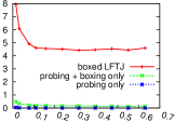
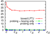
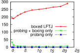
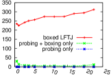
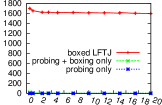
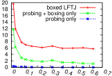
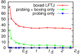
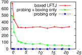
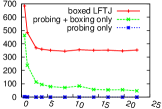
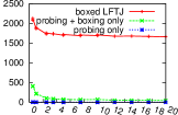
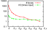
(a) LJ

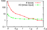
(b) ORKUT

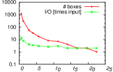
(c) RAND80

(d) RMAT80

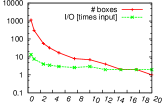
(e) TWITTER

Figure 7: Boxed LFTJ Analysis. On the X-Axis, we vary the amount of total memory available for boxing shown in GB. First row show total runtime in seconds without OS-level memory-restrictions and warm caches to evaluate the additional CPU work necessary for boxing. For performance in an out-of-core scenario, we enforce OS-level memory restrictions and have all caches cleared before execution in the second row. The third row shows the number of boxes and the amount of provisioned memory in multiples of the size of the input data. Omitted graphs for {RAND|RMAT}16 look like the “80” variants.

What CPU overhead does Boxing introduce? To measure the CPU overhead that is introduced by the boxing approach, we advise LFTJ to only use memory the size of a fraction of the input during execution—yet, we do not place any limit on the caches the operating system keeps for file operations. To further (almost completely) remove I/O, we prefix the execution by cat-ting all input data to /dev/null, which essentially pre-loads the Linux file-system cache. We now consider the two questions (i) What is the CPU overhead for probing and copying? and (ii) What is the overhead introduced by running LFTJ on individual boxes in comparison to running LFTJ on the whole input data. To answer the first question, we simply run three variants: (a) the full LFTJ, (b) probing and copying data into TrieArraySlices without running LFTJ, and (c) only probing without copying input data nor running LFTJ. Results are shown in the first row of Fig. 7. On the X-Axis, we vary the space available for boxing. The individual points range from $5,10,\dots$ up to $200\%$ of the input data size in TrieArray representation. We chose to range up to 200% since the input is essentially read twice by $\textnormal{LFTJ-}\Delta$: once for each of the dimensions $x$ and $y$.

Results. Answering question (i): We can see that the CPU work performed for probing and copying is very low in comparison to the work done by the join evaluation, even when the box sizes are limited to as little as $5\%$ of the size of the input. Answering (ii), we look at the red lines for LFTJ and compare the curve with the value at the far right as this one is achieved by using a single box. The real-world data sets behave as expected: starting at around 25%, they level out demonstrating that the CPU overhead is low if the available memory is not too much smaller than the input data size. Now, for the synthetic data sets, we see that unexpectedly, using more boxes reduces the CPU work (memory range 10%–200%). We speculate that this is because the boxed version might reduce the work done in binary searches for seek since the space that needs to be searched is smaller. Only at 5%, does this trend reverse and using more smaller boxes takes longer.

How well does Boxing do with limited memory? We are also interested in the performance of the boxing technique when disk I/O needs to be performed. Here, we run the same experiments as above but we clear all linux system caches (see Apx. C.1) before we start a run. We further use Linux’s cgroup feature to limit the total amount of RAM used for the program (data+executable) and any caches used by the operating system to buffer I/O on behalf of the program. As actual limit we use the value given to the boxing and shown on the X-Axis plus a fixed 100MB (that accounts for the output buffer and the size of the executable). Results are shown in the second row of Fig. 7. We see that probing is still very cheap even for the 5% memory setting; Provisioning the data now has noticeable costs for low-memory settings (25% and below). However, even then, it is mostly dominated by the time to actually perform the in-memory joins. This is even more so for the real-world data sets. Overall, with around 25% or more memory, boxed LFTJ’s performance stays constant indicating that I/O is not the bottleneck. For example, we can count all 37 billion triangles in the TWITTER dataset in around 29 minutes without I/O and only need up to 35 minutes with disk I/O.

In the third row of Fig. 7, we show number of boxes used as well as the total amount of memory copied for provisioning as a multiple of the TrieArray input size from Fig. 6. We see that the number of boxes is generally below 100 unless the memory is restricted to below 25%; similarly, we never copy more than 15x of the input data even for a 5% memory restriction. An example for how the boxes were chosen for the TWITTER data set is shown in Fig. 8. Each figure shows the front (x-y) plane of the 3-D input space. Darker pixels stand for more data of the represented area. We see that boxes become smaller around the more data-dense areas. See Apx. D for more details.

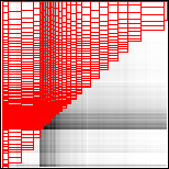
(a) 5%

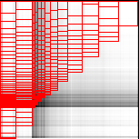
(b) 10%

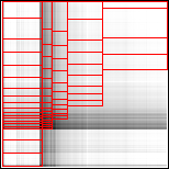
(c) 25%

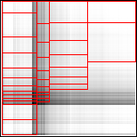
(d) 35%

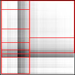
(e) 75%

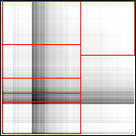
(f) 100%

Figure 8: Selected boxes for TWITTER dataset

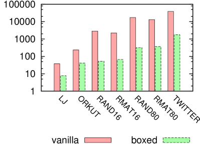
(a) Limit: 25% of input

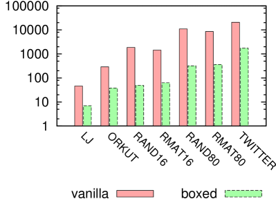
(b) Limit: 35% of input

Figure 9: Vanilla vs. Boxed LFTJ. For our LFTJ implementation based on TrieArrays. Y-Axis shows wall-clock runtime in seconds. Memory restricted as mentioned.

Last, we are interested in how the boxed LFTJ compares to a variant without our extension. Since LFTJ as presented in [36] is a family of algorithms that needs to be parameterized by how data is physically stored and how the TrieIterator operations are implemented, answering this question is hard since conclusions for one specific implementation of the data back-end might not hold for another. In particular, our approach of storing data in huge arrays and performing mostly binary searches over them might be particularly bad from an I/O perspective. However, having these considerations in mind, we also ran our version of LFTJ with the cgroup memory restrictions and a provisioning mode that does not copy the data but leaves it in memory-mapped files. The data is thus paged in (from the input file) by the Linux virtual memory system that using a standard replacement strategy. Results for this experiment are shown in Fig. 9: The average speed ratios of vanilla over boxed for the memory levels of 10%, 25%, and 35% are 65x, 30x, and 20x, respectively.

.

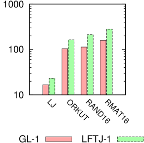
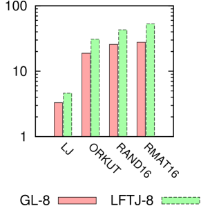
Figure 10: Performance Graphlab vs. Boxed LFTJ for single and multi threaded configurations. No resource limitations. Y-axis shows runtime in seconds.

How does boxed LFTJ compare to specialized best-in-class competitors for triangle listings? We compare to (1) the triangle counting algorithm presented in Shank’s dissertation [32] which has been implemented for the graph analysis framework Graphlab [16]. We chose this algorithm as our in-memory competitor since it supports multiple threads and was used in other comparisons [37] before. We also (2) compare to the MGT algorithm by Hu, Tao, and Chung [10] as the (to the best of our knowledge) currently best triangle listing algorithm in the out-of-core setting. Our results are shown in Fig. 10 and Fig. 11. The boxed LFTJ is on average 65% slower than Graphlab, both when run in single-threaded mode as well as in multi-threaded mode with 8 threads. Graphlab, being optimized for an in-memory setting with optional distribution, was not able to run any of our large data sets getting “stuck” once all of the 32GB of main memory and 32GB of swap space had been consumed.

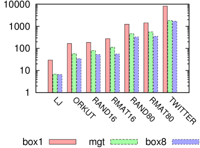
(a) Limit: 10% of input

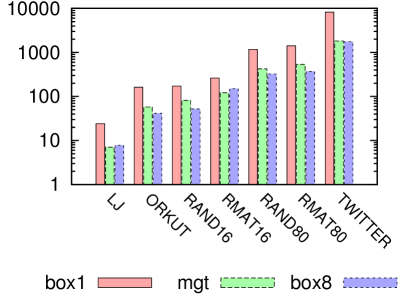
(b) Limit: 25% of input

Figure 11: Comparison: Boxed LFTJ (1,8 threads) vs. MGT (1 thread) with limited memory. Y-Axis shows wall-clock runtime in seconds.

Comparing to MGT (cf. Fig. 11): We used the cgroup-memory restrictions and cleaned caches for running MGT and boxed-LFTJ. When we run in single-threaded mode, then MGT outperforms boxed LFTJ by a factor of $3.1$, $2.9$, and $2.9$ in the configurations with 10%, 25%, and 35% of the memory, respectively. Due to time constraints, we did not run LFTJ in single-threaded mode for other configurations. When we allow LFTJ to utilize all of the 4 available cores, we are on average 47%, 22%, and 28%, respectively, faster than the single-threaded MGT. We have not investigated how well MGT parallelizes. Note that MGT internally uses only 32 bits as node identifiers (vs. our 64bit identifiers). Nevertheless, we used the same values to configure and limit the amount of memory for both MGT and LFTJ.

7 Related Work

Related work spans multiple areas at different levels of generality. From most broad to more specific:

The SociaLite effort [33, 34] at Stanford also proposes to use systems based on relational joins (in this case Datalog) for graph analysis. They show that declarative methods not only allow for more succinct programs but are also competitive, if not outperform typical other implementations. We did not compare our join performance with the SociaLite system as it is clearly more feature-rich; it is also Java-based which might or might not influence performance in ways orthogonal to our investigation. We note that the benchmarks presented in [33] and [34] that–among other queries–evaluate counting triangles did not use datasets as large as ours.

A worst-case optimal join algorithm has first been presented by Ngo et al. in [21] following the AGM bound [3] that bounds the maximum number of tuples that can be produced by a conjunctive join. Leapfrog Triejoin by Veldhuizen [36], the join algorithm we are using, has been shown to be worst-case optimal as well (modulo a log-factor). In fact, [36] showed that Leapfrog Triejoin is worst-case optimal (modulo log-factor) for more fine-grained families of inputs. Our work, especially on the worst-case optimality for graphs with limited arboricity was inspired by the worst-case optimal results in [36]. A good survey and description of this class of worst-case optimal join algorithms is [22], where the authors not only describe the AGM bound and its application, but also the original NPRR algorithm and LFTJ.

Most recently, Khamis, Ngo, Re, and Rudra proposed so-called beyond-worst-case-optimal join algorithms. Here, the performed work is not measured against a worst-case within a set family of inputs—but instead must be proportional to the size of a shortest proof of the results correctness. The idea was proposed by Ngo, Nguyen, Re and Rudra in [20]. Furthermore, [11] combines ideas from geometry and resolution transforming the algorithmic problem of computing joins to a geometric one. Following this line of research is very interesting as it might offer even better performance in practice.

Our boxing approach is most closely related to the classic block-nested loop join (BNLJ)[29]. An interesting avenue for future work would be to investigate how optimizations and results for the BNLJ transfer to the multi-predicate LFTJ.

Listing triangles in graphs is a well-researched area in computer science. For the in-memory context, see [13] for a recent survey. Triangle listing can also be reduced to matrix multiplication. Recent work that proposes new algorithms based on this approach is [4]. Chiba and Nishizeki [7] propose an in-memory triangle listing algorithm that runs in $O(|E|\alpha(G))$ matching the best possible bound we give in Section 4. To the best of our knowledge, our insight that this is the best possible theoretical bound for this class of graphs, is novel and thus provides new insights about these algorithms. Earlier, [26] already showed that enumerating all triangles in planar graphs is a linear-time problem.

Triangle listing in the out-of-core context: Following up on the MGT work [10], Rasmus and Silvestri investigate the I/O complexity of triangle listing [23]. They improve on the $I/O$ complexity of MGT from $O(|E|^{2}/(MB))$ to an expected $O(E^{3/2}/(\sqrt{M}B))$. They also give lower bounds and show that their algorithm is worst-case optimal by proving that any algorithm that enumerates $K$ triangles needs to use at least $\Omega(K/(\sqrt{M}B))$ I/Os. They also give a deterministic algorithm using a color coding technique. Investigating whether the techniques used could be generalized to general joins is a very interesting avenue for future work. Prior to [10], [17] proposed an algorithm whith an I/O complexity of $O(|E|+|E|^{1.5}/B)$; furthermore [9] proposed an algorithm with an I/O complexity of $O(|E|^{1.5}/B\cdot\log_{M/B}(|E|/B))$. Cheng et al. [6] study the general problem of finding maximal cliques. We did not benchmark against these algorithms since MGT dominated them by an order of magnitude.

Research has also been done to distribute triangle counting and other graph algorithms [1, 2], and approaches that use the MapReduce framework [27, 28, 35, 24].

8 Conclusion

For the well-studied problem of triangle listing, we have investigated how a general-purpose & worst-case optimal join algorithm compares against specialized approaches in the out-of-core context. By using Leapfrog Triejoin, we were able to devise a strategy that not only allows for good theoretical bounds in terms of I/O and CPU costs but we also demonstrated very good performance: For very large input graphs of 1.2 billion edges and more, LFTJ counts triangles with a speed of 4 million input edges per second for uniformly random data; and performs a complete count of the 35 billion triangles in the twitter dataset in little over 25 minutes on a standard 4-core desktop machine while limiting the available main memory to around 5GB. Our positive results can be interpreted as a confirmation for the database community’s theme of creating systems to empower (domain-expert) users via declarative query interfaces while providing very good performance.

Acknowledgements. We thank Ken Ross and Haicheng Wu for comments on an earlier draft; and we thank the anonymous reviewers for their comments.

Appendix A Leapfrog Join and
Leapfrog Triejoin

Algorithm 3 Leapfrog join of $n$ unary relations [36]

1:in: $\mathsf{Array\;of}$ $\mathsf{LinearIterators}$ Iters[0..n-1]

2:variables: $\mathsf{int}$ $i$, $\mathsf{bool}$ atEnd

3:procedure lfj-init( )

4:     if any iterator in Iters[0..n-1] is atEnd( ) then

5:         atEnd $\leftarrow$ true $\triangleright$ Some input is empty

6:     else

7:         sort Iters[0..n-1] increasingly by value( )

8:         $\textnormal{$i$}\leftarrow 0$ ; atEnd $\leftarrow$ false

9:         lfj-search( )      

10:procedure lfj-search( )

11:     while true do

12:         if Iters[$\textnormal{$i$}-1\mod n$ ].atEnd( ) then

13:              atEnd $\leftarrow$ true

14:              return $\triangleright$ No tuple can be found anymore          

15:         max_value $\leftarrow$ Iters[$\textnormal{$i$}-1\mod n$ ].value( )

16:         min_value $\leftarrow$ Iters[$i$].value( )

17:         if min_value = max_value then

18:              return $\triangleright$ Found tuple in intersection

19:         else

20:              Iters[$i$].seek(max_value) ; $\textnormal{$i$}\leftarrow\textnormal{$i$}+1\mod n$               

21:procedure lfj-next( )

22:     Iters[$i$].next( ) ; $\textnormal{$i$}\leftarrow\textnormal{$i$}+1\mod n$

23:     lfj-search( )

24:procedure lfj-seek(val)

25:     Iters[$i$].seek(val) ; $\textnormal{$i$}\leftarrow\textnormal{$i$}+1\mod n$

26:     lfj-search( )

27:function lfj-value( ): return Iters[0].value( )

28:function lfj-atEnd( ): return atEnd

Algorithm 4 Leapfrog Triejoin with $n$ variables [36]

1:in: $\mathsf{Array\;of}$ $\mathsf{Set\,of\,LeapfrogJoins}$ Lfs[1..n]

2:variables: $\mathsf{int}$ $d$$\triangleright$ Current depth

3:procedure lftj-init( ): $\textnormal{$d$}\leftarrow 0$

4:procedure lftj-open( )

5:     $\textnormal{$d$}\leftarrow\textnormal{$d$}+1$

6:     for all $iter$ used in Lfs[$d$] do: $iter$.open( )      

7:     Lfs[$d$].lfj-init( )

8:procedure lftj-close( )

9:     for all $iter$ used in Lfs[$d$] do: $iter$.close( )      

10:     $\textnormal{$d$}\leftarrow\textnormal{$d$}-1$

11:procedure lftj-next( ): Lfs[$d$].lfj-next( )

12:procedure lftj-seek(v): Lfs[$d$].lfj-seek(v)

13:function lftj-value( ): return Lfs[$d$].lfj-value( )

14:function lftj-atEnd( ): return Lfs[$d$].lfj-atEnd( )

A.1 TrieIterator Example

A TrieIterator is initialized to the root node $r$. Methods for vertical navigation are: open() for moving “down” to the first children of the current node and close() for moving “up” to the parent of the current node. Horizontally, movement is restricted to direct siblings, which are accessed via the LinearIterator interface that comprises the methods atEnd, next, seek, and value. It is convenient to think of the $l$ children of a node $n$ to be stored increasingly sorted in an array $A$ of size $l$. The methods bool atEnd() returns true if the iterator is positioned after the last element (eg., at position $l$). The method next() requests to move to the next element; atEnd will be true if the iterator was at the last position already (e.g., calling next() at position $l-1$). The method seek(T $v$) can be used to forward-position the iterator to the element with value $v$; if $v$ is not in $A$, then the iterator is placed at the element with the smallest value $w>v$, or atEnd if no such $w$ exists. Finally, data is accessed at granularity of a single domain element via the method T value(), which returns the element at the current position. The methods open, next, seek, and value may only be called if atEnd() is false; furthermore, the value $v$ given to seek(v) must be at least value(); and value() must not be called at the root node $r$.

Example 20 (TrieIterator Navigation).

See Figure 1(b). The iterator is initially positioned at r; open() moves it to a, followed by next() to b. Here, open() moves to u; next() to v; and a seek(w) will position the iterator to z since z is the smallest among u,v,z which is larger than w. A call to next() causes atEnd() to return true after which close() would be the only allowed operation, moving the iterator back to b.

A.2 Leapfrog TrieJoin Procedure

Given a join description as a Datalog rule body with $m$ atoms and $n$ variables. For each of the $m$ atoms, a single TrieIterator is created. Furthermore, LFTJ maintains an array of $n$ Leapfrog joins—one join for each variable. The LFJ for variable $x_{i}$ uses pointers to the TrieIterators for atoms that mention the variable $x_{i}$. Overall, LFTJ is implemented as a TrieIterator itself (see Algorithm 4). A variable $d$ remembers at which level of the output trie the iterator is positioned. The horizontal navigation methods manipulate $d$, open and close the appropriate TrieIterators, and initialize the Leapfrog joins. The linear iterator methods are then simply delegated to the LFJ which computes the appropriate intersections.

Appendix B Proofs

.$\begin{array}[]{rr}\mathbf{E:}\\ \hline\cr\hline\cr 0,&24\\ 1,&20\\ 2,&16\\ 3,&12\\ 4,&8\\ 5,&4\\ \hline\cr 6,&24\\ 7,&20\\ ..&..\\ \hline\cr 18,&24\\ ..&..\\ 23,&4\\ \hline\cr 24,&24\end{array}$.

(a) Graph $G$

.$\begin{array}[]{rrr|rr||r}a&b&c&D(a)&D(b)&\mathbf{I/O}\\ \hline\cr\hline\cr 0&&&24&&\\ 0&24&&24&24&1\\ 0&24&24&24&24&1\\ \hline\cr 1&&&20&&\\ 1&20&&20&16&1\\ 1&20&-&20&16&1\\ \hline\cr 2&&&16&&\\ 2&16&&16&8&1\\ 2&16&-&16&8&1\\ \hline\cr 3&&&12&&\\ 3&12&&12&24&1\\ 3&12&-&12&24&1\\ \hline\cr..&..&..&..&..\end{array}$ .

(b) $\textnormal{LFTJ-}\Delta$ steps when running on $G$

Figure 12: Example input graph that causes $\textnormal{LFTJ-}\Delta$ to use many I/Os. Parameters: $M=20$, $B=4$ and graph with $N=24$ edges.

B.1 Proof for Prop. 4

Consult Fig. 12(b). The variable assignments for $x:\!\!\leavevmode\resizebox{5.71527pt}{0.0pt}{=}\,a$, $y:\!\!\leavevmode\resizebox{5.71527pt}{0.0pt}{=}\,b$, and $z:\!\!\leavevmode\resizebox{5.71527pt}{0.0pt}{=}\,c$ as well as the corresponding neighbors $D(a)$ and $D(b)$ are shown. Each node in $V_{1}$ causes two block $I/O$s. Further, the block storing the node with id 24 of $V_{1}$ will be evicted when $x=5$ and $y=4$ or earlier, and the last block with $24$ is thus repeatedly loaded when $x=6$, $x=12$, and $x=18$.

Detailed proof sketch for general case: The outer loop in line 1 of Algorithm 1 ranges from $0$ to $N$. For each value $x:\!\!\leavevmode\resizebox{5.71527pt}{0.0pt}{=}\,a$, we then join $a$’s neighbors with $V_{1}$ (line 2) to obtain bindings for $y$. Since each node $a$ has exactly one neighbor $b$, this essentially performs a lookup of $b$ in the first column of $E$. Now, since we spaced the second values in $E$ with a distance of $B$ apart, locating each $b$ within $E$ incurs at least one I/O. Also, since the second values in $E$ repeat in groups of size $T$, the blocks needed for the second group will have been evicted from memory before they are needed, resulting in a single I/O for each tuple in $E$. The last step is to intersect the neighbors of $a$ with the neighbors of $b$. In our TrieArray representation, this will incur another I/O.

B.2 Proof for Proposition 16

The bound on the runtime can easily be obtained from the worst-case optimality wrt. input sizes of LFTJ (Corollary 4.3 in [36]) and the fractional edge-cover bound [3]: For any three binary relations $R$, $S$, $T$ the result size $|Q|$ of the join $Q(x,y,z)\leftarrow R(x,y),S(y,z),T(x,z)$ is limited according to the fractional edge cover [3]. If the sizes of $R$, $S$, and $T$ agree than $|Q|$ is at most $n^{1.5}$ with $n=|R|=|S|=|T|$; adding the log-factor, we obtain the desired bound of $O(\log|E||E|^{1.5})$.

The complexity is optimal modulo the log-factor since a graph with $|E|$ edges can have $\Omega(|E|^{1.5})$ triangles.

B.3 Proof for Theorem 17

Let $\hat{\alpha}$ be as required. We now analyze the work done by $\textnormal{LFTJ-}\Delta$ on a graph $G$ with its directed version ${G}^{\star}=(V,E)$ (possibly obtained via a $O(|E|\log|E|)$ preprocessing. Let $V_{1}$ be all nodes in $E$ that have an outgoing edge as usual. It is useful to also consult Fig. 1 for an explanation of which Leapfrog joins are executed during $\textnormal{LFTJ-}\Delta$. We now count the steps at each variable:

• At level $x$: We Leapfrog-join $V_{1}$ with itself yielding a bound of $O(|E|\log|E|)$ based on the requirements for the TrieIterator operations (see Section 2.1).

• At level $y$: for each $x\in V_{1}$, a leapfrog-join is performed between $D(x)$ and $V_{1}$. As usual, $D(x)$ are the followers of $x$, i.e., $D(x)=\{y\,|\,(x,y)\in E\}$. Summing up all cost and using that the runtime of a leapfrog-join between two relations of size $s_{1}$ and $s_{2}$, respectively, is bound by $O(\log(\max\{s_{1},s_{2}\})\cdot\min\{s_{1},s_{2}\})$, we obtain:

  $$\begin{array}[]{llll}&O(&\sum\limits_{x\in V_{1}}\log(\max\{d_{x},|V_{1}|\})\min{\{d_{x},|V_{1}|\}}&)\\ \subseteq&O(&\log|V|\cdot\sum\limits_{x\in V_{1}}|D(x)|&)\\ \subseteq&O(&|E|\log|V|&)\\ \subseteq&O(&|E|\log|E|&)\end{array}$$

• At level $z$: Here, for (at most) each edge $(x,y)$ in $E$ we leapfrog join the neighbors of $x$ with the neighbors of $y$. We thus incur the work:

  $$\begin{array}[]{llll}&O(&\sum\limits_{(x,y)\in E}\log(\max\{d_{x},d_{y}\})\min\{d_{x},d_{y}\}&)\\ \subseteq&O(&\sum\limits_{(x,y)\in E}\log(\max\limits_{v\in V}\{d_{v}\})\min\{d_{x},d_{y}\}&)\\ \subseteq&O(&\log(\max\limits_{x\in V}\{d_{x}\})\cdot\sum\limits_{(x,y)\in E}\min\{d_{x},d_{y}\}&)\\ \subseteq&O(&\log|E|\cdot\sum\limits_{(x,y)\in E}\min\{d_{x},d_{y}\}&)\\ \end{array}$$

  As Lemma 2, Chiba and Nishizeki [7] observed that for any graph $G=(V,E)$, the sum $\sum_{(x,y)\in E}\min\{d_{x},d_{y}\}$ is bounded by $2\alpha(G)|E|$. Since $\alpha(G)\leq\hat{\alpha}(|E|)$ and because $\hat{\alpha}$ is monotonically increasing, we can bound the work by $O(\log|E|\hat{\alpha}(|E|)|E|)$, finishing the proof.

B.4 Proof for Theorem 19

We first show:

Lemma 21.

Let $\hat{\alpha}:\mathbb{N}\rightarrow\mathbb{N}^{+}$ be an arbitrary monotonically increasing, computable function. For any $m\in\mathbb{N}$ there exists a graph with $m$ edges and arboricity at most $\hat{\alpha}(m)$ with at least $\frac{2}{3}m\hat{\alpha}(m)-\frac{2}{3}m-\frac{4}{3}\hat{\alpha}(m)^{3}-\frac{2}{3}\hat{\alpha}(m)^{2}$ triangles.

Proof.

Informal overview of technique. To get many triangles, we use fully connected graphs $K_{k}$; to stay under the arboricity limit, we choose $k$ appropriately; to get many edges, we just union many of these $K_{k}$ into the graph, and then filling up with singleton edges. The math works out to the above quantity.

Formal proof. Let $\hat{\alpha}$ be as required. Fix an $m\in\mathbb{N}$. Let $k=2\hat{\alpha}(m)$. Note that the fully connected graphs $K_{k}$ with $k$ nodes have $l=k(k-1)/2$ edges. We construct a graph $G$ by packing as many $K_{k}$ as we can fit into our “$m$-edges budget” and filling up the rest with unconnected edges: Let $n=\left\lfloor m/l\right\rfloor$, let $G$ be the graph composed of $n$ instances of $K_{k}$ and $m-nl$ single edges not connected to anything else. To complete the proof, we show: (1) The arboricity of $G$ is $\hat{\alpha}(m)$, and (2) $G$ has at least $\frac{2}{3}m\hat{\alpha}(m)-\frac{2}{3}m-\frac{4}{3}\hat{\alpha}(m)^{3}-\frac{2}{3}\hat{\alpha}(m)^{2}$ triangles.

Showing (1). The classic Nash-Williams result [19] states that for any graph $G$, its arboricity $\alpha(G)$ is characterized by the maximum edge-node ratio among all its subgraphs:

$$\alpha(G)=\max\limits_{S\textnormal{ is subgraph of }G}\left\{\left\lceil{\frac{|E(S)|}{|V(S)|-1}}\right\rceil\right\}$$

It can easily be verified that choosing a $K_{k}$ as subgraph maximizes the ratio. Thus, $\alpha(G)=\alpha(K_{k})=\lceil k/2\rceil=\hat{\alpha}(m)$.

Showing (2) As short-hand let $\alpha=\hat{\alpha}(m)$, and let $m^{\prime}=nl$, which is the largest integer multiple of $l$ that is not larger than $m$. Each $K_{k}$ has ${k\choose 3}=k(k-1)(k-2)/6=l(k-2)/3$ triangles, and we have $n$ of them, totaling in

$$\begin{array}[]{lll}nl(k-2)/3&=\frac{1}{3}m^{\prime}(k-2)\\ &\hfill\triangleright\;k=2\alpha\\ &=\frac{2}{3}m^{\prime}(\alpha-1)\\ &\hfill\triangleright\;m^{\prime}\geq m-l+1\\ &\geq\frac{2}{3}(m-l+1)(\alpha-1)\\ \\ &=\frac{2}{3}(m\alpha-m-l\alpha+l+\alpha-1)\\ \\ &=\frac{2}{3}(m\alpha-m-l(\alpha+1)+\alpha-1)\\ &\hfill\triangleright\;l=2\alpha^{2}-\alpha\\ &=\frac{2}{3}(m\alpha-m-(2\alpha^{2}-\alpha)(\alpha+1)+\alpha-1)\\ &\\ &=\frac{2}{3}(m\alpha-m-(2\alpha^{3}+\alpha^{2}-\alpha)+\alpha-1)\\ &\\ &=\frac{2}{3}(m\alpha-m-2\alpha^{3}-\alpha^{2}+\alpha+\alpha-1)\\ &\\ &=\frac{2}{3}(m\alpha-m-2\alpha^{3}-\alpha^{2}+2\alpha-1)\\ &\\ &=\frac{2}{3}(m\alpha-m-2\alpha^{3}-(\alpha-1)^{2})\\ &\hfill\triangleright\;\alpha\geq 1\\ &\geq\frac{2}{3}(m\alpha-m-2\alpha^{3}-\alpha^{2})\\ &\\ &=\frac{2}{3}m\alpha-\frac{2}{3}m-\frac{4}{3}\alpha^{3}-\frac{2}{3}\alpha^{2}\end{array}$$

triangles as required.

We proof Theorem 19 indirect. Let $\hat{\alpha}:\mathbb{N}\rightarrow\mathbb{N}^{+}$ be an arbitrary, monotonically increasing, computable function, not identical to 1, that is in $o(\sqrt{n})$. And, let $\mathcal{A}$ be an algorithm that lists all triangles in graphs $G=(V,E)$ with $\alpha(G)\leq\hat{\alpha}(|E|)$ in $o(|E|\hat{\alpha}(|E|))$ time. Let $T_{\alpha}(m):\mathbb{N}\rightarrow\mathbb{N}$ be the maximal number of steps $\mathcal{A}$ performs on any graph $G=(V,E)$ with $|E|\leq m$ and $\alpha(G)\leq\alpha$.

Since $\mathcal{A}$ runs in $o(|E|\hat{\alpha}(|E|))$ time: choose $\epsilon_{0}=1/16$ and let $m_{0}$ be such that for all $m\geq m_{0}$ we have:

$$T_{\alpha}(m)\leq\frac{1}{16}m\hat{\alpha}(m)\quad\quad\textnormal{ for all }m\geq m_{0}$$ (1)

From $\hat{\alpha}\in o(\sqrt{n})$: choose $\epsilon_{1}=1/\sqrt{8}$ and let $m_{1}$ such that for all $m\geq m_{1}$ we have $\hat{\alpha}(m)\leq\frac{1}{\sqrt{8}}\sqrt{m}$.

Now, let $m^{\star}\in\mathbb{N}$ be a large enough number such that (1) $m^{\star}\geq 8$, (2) $m^{\star}\geq m_{0}$, (3) $m^{\star}\geq m_{1}$, and (4) $\hat{\alpha}(m^{\star})\geq 2$. We can satisfy all conditions since $\alpha$ maps into $\mathbb{N}^{+}$, is monotonically increasing, and is not identical to 1. We apply Lemma 21 with our $\hat{\alpha}$ for $m^{\star}$, and conclude there is a graph $G^{\star}$ with $m^{\star}$ edges and arboricity at most $\hat{\alpha}(m^{\star})$ with at least $s(m^{\star})=\frac{2}{3}m^{\star}\hat{\alpha}(m^{\star})-\frac{2}{3}m^{\star}-\frac{4}{3}\hat{\alpha}(m^{\star})^{3}-\frac{2}{3}\hat{\alpha}(m^{\star})^{2}$ triangles. Clearly, $\mathcal{A}$ needs to take at least $s(m^{\star})$ steps on $G^{\star}$. Thus:

$$\begin{array}[]{llll}T_{\alpha}(m^{\star})&\geq&\frac{2}{3}m^{\star}\hat{\alpha}(m^{\star})-\frac{2}{3}m^{\star}-\frac{4}{3}\hat{\alpha}(m^{\star})^{3}-\frac{2}{3}\hat{\alpha}(m^{\star})^{2}\textnormal{{\color[rgb]{1,1,1}xx}}\\ &&\hfill\triangleright\;\hat{\alpha}(m^{\star})\leq\frac{1}{\sqrt{8}}\sqrt{m^{\star}}\\ &\geq&\frac{2}{3}m^{\star}\hat{\alpha}(m^{\star})-\frac{2}{3}m^{\star}-\frac{1}{6}\hat{\alpha}(m^{\star})m^{\star}-\frac{1}{12}m^{\star}\\ \\ &\geq&\frac{1}{2}m^{\star}\hat{\alpha}(m^{\star})-\frac{3}{4}m^{\star}\\ &&\hfill\triangleright\;\hat{\alpha}(m^{\star})\geq 2\\ &\geq&\frac{1}{2}m^{\star}\hat{\alpha}(m^{\star})-\frac{3}{8}m^{\star}\hat{\alpha}(m^{\star})\\ &&\hfill\\ &\geq&\frac{1}{8}m^{\star}\hat{\alpha}(m^{\star})\\ &&\hfill\triangleright\;m^{\star}\geq 8,\hat{\alpha}(m^{\star})\geq 2\\ &\geq&\frac{1}{16}m^{\star}\hat{\alpha}(m^{\star})+1\\ &&\\ &>&\frac{1}{16}m^{\star}\hat{\alpha}(m^{\star})\hfill\textnormal{contradicts }\eqref{eqUpperBound}$\@qedbox{}$\\ \end{array}$$

Appendix C Systems Aspects

C.1 Caches and Limiting Resident Memory

To clear Linux file caches we used as root:

 sync && echo 3 > /proc/sys/vm/drop_caches

We restricted the memory that a process uses for any reason (data, heap, program, caches, etc) using Linux cgroups. Investigating later via top, confirms that only the allowed resident memory is used by the process. We used as root commands such as:

 # create a group
 mkdir -p /sys/fs/cgroup/memory/limit_mem
 # add process to group
 echo $PID_OF_PROCESS \
    > /sys/fs/cgroup/memory/limit_mem/tasks
 # limit memory
 echo $LIMIT_BYTES \
    > /sys/fs/cgroup/memory/limit_mem/\
      memory.limit_in_bytes

Appendix D More details for Fig. 8

The input space for $\textnormal{LFTJ-}\Delta$ is 3-dimensional. We box for $\textnormal{{atoms}}[1]$ = $\{E(x,y),E(x,z)\}$ and $\textnormal{{atoms}}[2]$ = $\{E(y,z)\}$. Since there were no spills, intervals for dimension $z$ are always $[-\infty\!\cdot\!\cdot\infty]$. The figures show how these boxes are created by projecting the 3-D input space onto the x-y plane. Darker pixels indicate areas where there is more data. In particular, the image was created as follows: For $E(x,y)$ of the directed graph for the twitter dataset which can be viewed as a point-set in 2D space, create a 2D histogram $H$ with 150x150 bins. Then, because we slice along the first dimension and collect the nodes plus their neighbors, we aggregate over $H$’s second dimension (eg, $y$) values to obtain a 1D histogram $D$ showing the total number of neighbors the nodes in a certain bin have. We then spread this 1D histogram into a 2D space by setting the value at position $x,y$ to $D(x)+D(y)$. This “image” is indicative of the total amount of data for a rectangular box. As a last step, we equalize the histogram and map into greyscale to have a prettier picture. The red boxes are then drawn on top according to the made provisioning decisions during the boxing procedure. In the picture the $x$-axis goes from bottom left to bottom right, the $y$ axis from bottom-left to top-left—the same way as in Fig. 2(e). Note, that the number of columns corresponds to how often we need to load the input data at level $y$.

References

- [1] F. N. Afrati, D. Fotakis, and J. D. Ullman. Enumerating subgraph instances using map-reduce. In Data Engineering (ICDE), 2013 IEEE 29th International Conference on, pages 62–73. IEEE, 2013.
- [2] F. N. Afrati and J. D. Ullman. Optimizing joins in a map-reduce environment. In Proceedings of the 13th International Conference on Extending Database Technology, pages 99–110. ACM, 2010.
- [3] A. Atserias, M. Grohe, and D. Marx. Size bounds and query plans for relational joins. In Foundations of Computer Science, 2008. FOCS’08. IEEE 49th Annual IEEE Symposium on, pages 739–748. IEEE, 2008.
- [4] A. Björklund, R. Pagh, V. Williams, and U. Zwick. Listing triangles. In J. Esparza, P. Fraigniaud, T. Husfeldt, and E. Koutsoupias, editors, Automata, Languages, and Programming, volume 8572 of Lecture Notes in Computer Science, pages 223–234. Springer Berlin Heidelberg, 2014.
- [5] D. Chakrabarti, Y. Zhan, and C. Faloutsos. R-MAT: A recursive model for graph mining. In SDM, volume 4, pages 442–446. SIAM, 2004.
- [6] J. Cheng, Y. Ke, A. W.-C. Fu, J. X. Yu, and L. Zhu. Finding maximal cliques in massive networks. ACM Transactions on Database Systems (TODS), 36(4):21, 2011.
- [7] N. Chiba and T. Nishizeki. Arboricity and subgraph listing algorithms. SIAM Journal on Computing, 14(1):210–223, 1985.
- [8] S. Chu and J. Cheng. Triangle listing in massive networks and its applications. In Proceedings of the 17th ACM SIGKDD international conference on Knowledge discovery and data mining, pages 672–680. ACM, 2011.
- [9] R. Dementiev. Algorithm engineering for large data sets. PhD thesis, Saarland University, 2006.
- [10] X. Hu, Y. Tao, and C.-W. Chung. Massive graph triangulation. In Proceedings of the 2013 international conference on Management of data, pages 325–336. ACM, 2013.
- [11] M. A. Khamis, H. Q. Ngo, C. Ré, and A. Rudra. A resolution-based framework for joins: Worst-case and beyond. CoRR, abs/1404.0703, 2014.
- [12] H. Kwak, C. Lee, H. Park, and S. Moon. What is Twitter, a social network or a news media? In WWW ’10: Proceedings of the 19th international conference on World wide web, pages 591–600, New York, NY, USA, 2010. ACM.
- [13] M. Latapy. Main-memory triangle computations for very large (sparse (power-law)) graphs. Theoretical Computer Science, 407(1):458–473, 2008.
- [14] J. Leskovec and A. Krevl. SNAP Datasets: Stanford large network dataset collection. http://snap.stanford.edu/data, June 2014.
- [15] M. C. Lin, F. J. Soulignac, and J. L. Szwarcfiter. Arboricity, h-index, and dynamic algorithms. Theoretical Computer Science, 426:75–90, 2012.
- [16] Y. Low, D. Bickson, J. Gonzalez, C. Guestrin, A. Kyrola, and J. M. Hellerstein. Distributed graphlab: A framework for machine learning and data mining in the cloud. Proc. VLDB Endow., 5(8):716–727, Apr. 2012.
- [17] B. Menegola. An external memory algorithm for listing triangles. Technical report, Universidade Federal do Rio Grande do Sul, 2010.
- [18] A. Mislove, M. Marcon, K. P. Gummadi, P. Druschel, and B. Bhattacharjee. Measurement and Analysis of Online Social Networks. In Proceedings of the 5th ACM/Usenix Internet Measurement Conference (IMC’07), San Diego, CA, October 2007.
- [19] C. S. A. Nash-Williams. Decomposition of finite graphs into forests. Journal of the London Mathematical Society, s1-39(1):12, 1964.
- [20] H. Q. Ngo, D. T. Nguyen, C. Ré, and A. Rudra. Beyond worst-case analysis for joins with minesweeper. CoRR, abs/1302.0914, 2014.
- [21] H. Q. Ngo, E. Porat, C. Ré, and A. Rudra. Worst-case optimal join algorithms:[extended abstract]. In Proceedings of the 31st symposium on Principles of Database Systems, pages 37–48. ACM, 2012.
- [22] H. Q. Ngo, C. Re, and A. Rudra. Skew strikes back: New developments in the theory of join algorithms. ACM SIGMOD Record, 42(4):5–16, 2014.
- [23] R. Pagh and F. Silvestri. The input/output complexity of triangle enumeration. In Proceedings of the 33rd ACM SIGMOD-SIGACT-SIGART Symposium on Principles of Database Systems, PODS’14, Snowbird, UT, USA, June 22-27, 2014, pages 224–233, 2014.
- [24] R. Pagh and C. E. Tsourakakis. Colorful triangle counting and a mapreduce implementation. Inf. Process. Lett., 112(7):277–281, 2012.
- [25] G. Palla, I. Derényi, I. Farkas, and T. Vicsek. Uncovering the overlapping community structure of complex networks in nature and society. Nature, 435(7043):814–818, 2005.
- [26] C. H. Papadimitriou and M. Yannakakis. The clique problem for planar graphs. Information Processing Letters, 13(4–5):131 – 133, 1981.
- [27] H.-M. Park, F. Silvestri, U. Kang, and R. Pagh. Mapreduce triangle enumeration with guarantees. Proc. 23rd CIKM, 2014.
- [28] L. Qin, J. X. Yu, L. Chang, H. Cheng, C. Zhang, and X. Lin. Scalable big graph processing in mapreduce. In Proceedings of the 2014 ACM SIGMOD international conference on Management of data, pages 827–838. ACM, 2014.
- [29] R. Ramakrishnan and J. Gehrke. Database management systems, volume 3. McGraw-Hill New York, 2003.
- [30] J. W. Raymond, E. J. Gardiner, and P. Willett. Rascal: Calculation of graph similarity using maximum common edge subgraphs. The Computer Journal, 45(6):631–644, 2002.
- [31] N. Rhodes, P. Willett, A. Calvet, J. B. Dunbar, and C. Humblet. Clip: similarity searching of 3d databases using clique detection. Journal of chemical information and computer sciences, 43(2):443–448, 2003.
- [32] T. Schank. Algorithmic aspects of triangle-based network analysis. Phd in computer science, University Karlsruhe, 2007.
- [33] J. Seo, S. Guo, and M. S. Lam. Socialite: Datalog extensions for efficient social network analysis. In 29th International Conference on Data Engineering (ICDE), pages 278–289. IEEE, 2013.
- [34] J. Seo, J. Park, J. Shin, and M. S. Lam. Distributed socialite: a datalog-based language for large-scale graph analysis. Proceedings of the VLDB Endowment, 6(14):1906–1917, 2013.
- [35] S. Suri and S. Vassilvitskii. Counting triangles and the curse of the last reducer. In Proceedings of the 20th international conference on World wide web, pages 607–614. ACM, 2011.
- [36] T. L. Veldhuizen. Triejoin: A simple, worst-case optimal join algorithm. In Proc. 17th International Conference on Database Theory (ICDT), Athens, Greece, March 24-28, 2014., pages 96–106, 2014.
- [37] H. Wu, D. Zinn, M. Aref, and S. Yalamanchili. Multipredicate join algorithms for accelerating relational graph processing on GPUs. Fifth International Workshop on Accelerating Data Management Systems Using Modern Processor and Storage Architectures (ADMS 2014), September 2014.
- [38] J. Yang and J. Leskovec. Defining and evaluating network communities based on ground-truth. CoRR, abs/1205.6233, 2012.
- [39] 2010 Twitter data set. Downloaded Oct 2014 from http://an.kaist.ac.kr/traces/WWW2010.html.
- [40] https://developer.nvidia.com/cuda-gpus.
- [41] R-MAT Data generator. http://www.cse.psu.edu/ madduri/software/GTgraph/.